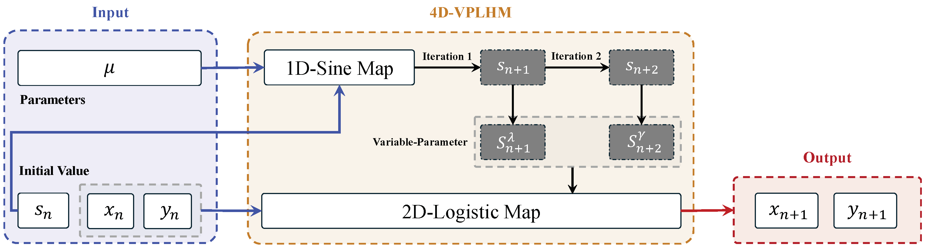
Figure 1.
The model structure of four-dimensional variable-parameter Logistic hyperchaotic map.
Figure 1.
The model structure of four-dimensional variable-parameter Logistic hyperchaotic map.
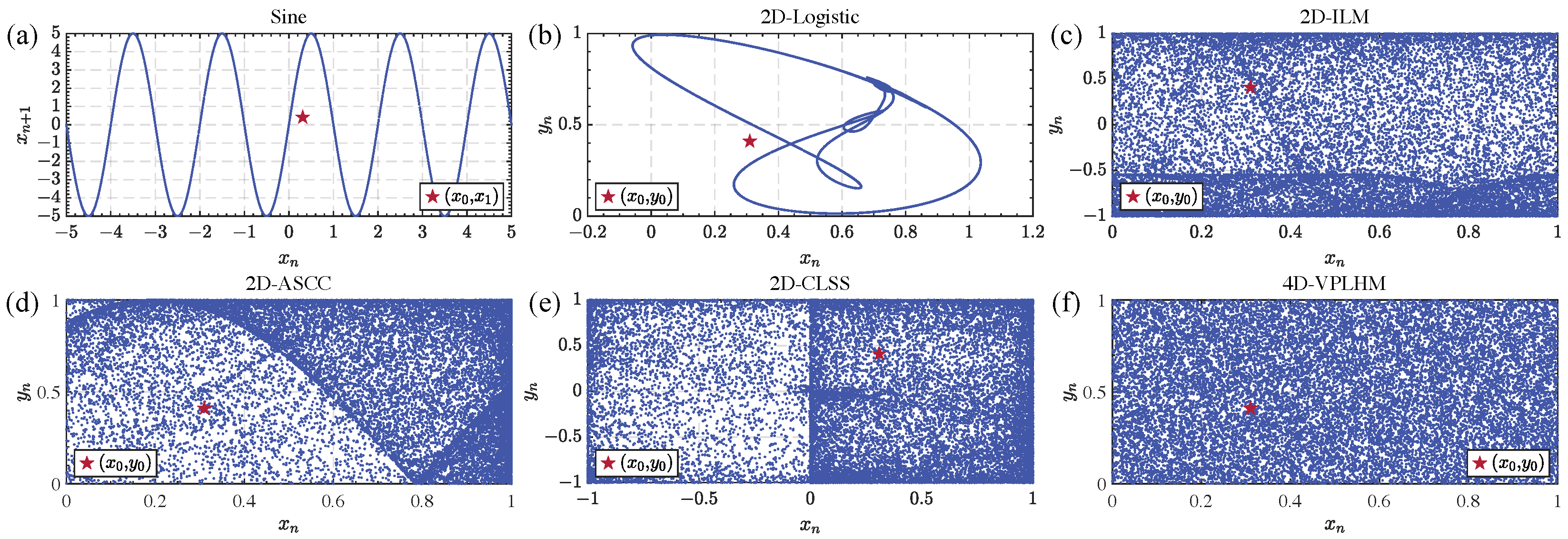
Figure 2.
Comparison results of the trajectory maps of chaotic systems: (a) Sine chaotic system, (b) 2D-Logistic chaotic system, (c) 2D-ILM chaotic system, (d) 2D-ASCC chaotic system, (e) 2D-CLSS chaotic system, (f) 4D-VPLHM chaotic system.
Figure 2.
Comparison results of the trajectory maps of chaotic systems: (a) Sine chaotic system, (b) 2D-Logistic chaotic system, (c) 2D-ILM chaotic system, (d) 2D-ASCC chaotic system, (e) 2D-CLSS chaotic system, (f) 4D-VPLHM chaotic system.
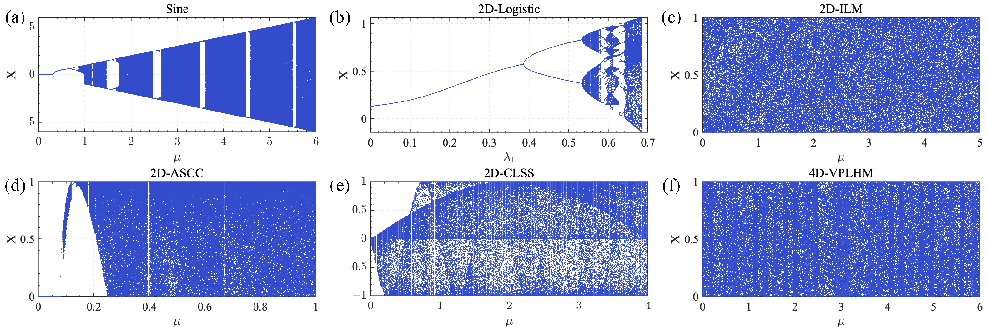
Figure 3.
Comparison results of bifurcation diagrams of chaotic system: (a) Sine chaotic system, (b) 2D-Logistic chaotic system, (c) 2D-ILM chaotic system, (d) 2D-ASCC chaotic system, (e) 2D-CLSS chaotic system, (f) 4D-VPLHM chaotic system.
Figure 3.
Comparison results of bifurcation diagrams of chaotic system: (a) Sine chaotic system, (b) 2D-Logistic chaotic system, (c) 2D-ILM chaotic system, (d) 2D-ASCC chaotic system, (e) 2D-CLSS chaotic system, (f) 4D-VPLHM chaotic system.
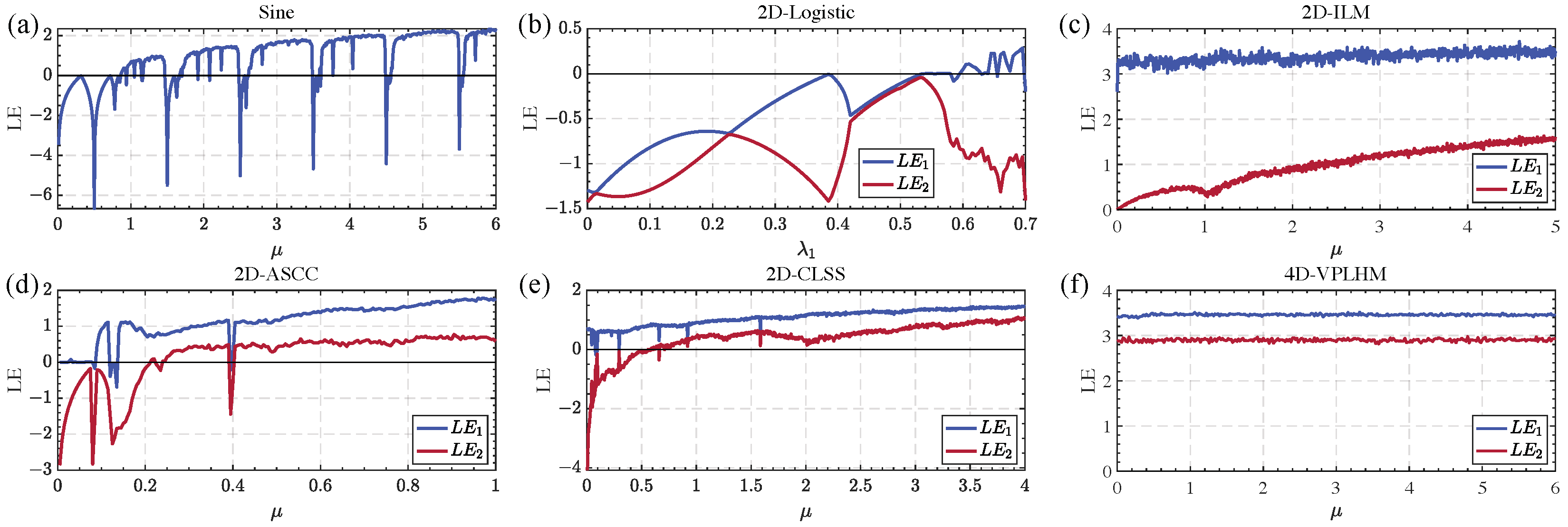
Figure 4.
Results of Lyapunov exponent comparison for chaotic systems: (a) Sine chaotic system, (b) 2D-Logistic chaotic system, (c) 2D-ILM chaotic system, (d) 2D-ASCC chaotic system, (e) 2D-CLSS chaotic system, (f) 4D-VPLHM chaotic system.
Figure 4.
Results of Lyapunov exponent comparison for chaotic systems: (a) Sine chaotic system, (b) 2D-Logistic chaotic system, (c) 2D-ILM chaotic system, (d) 2D-ASCC chaotic system, (e) 2D-CLSS chaotic system, (f) 4D-VPLHM chaotic system.
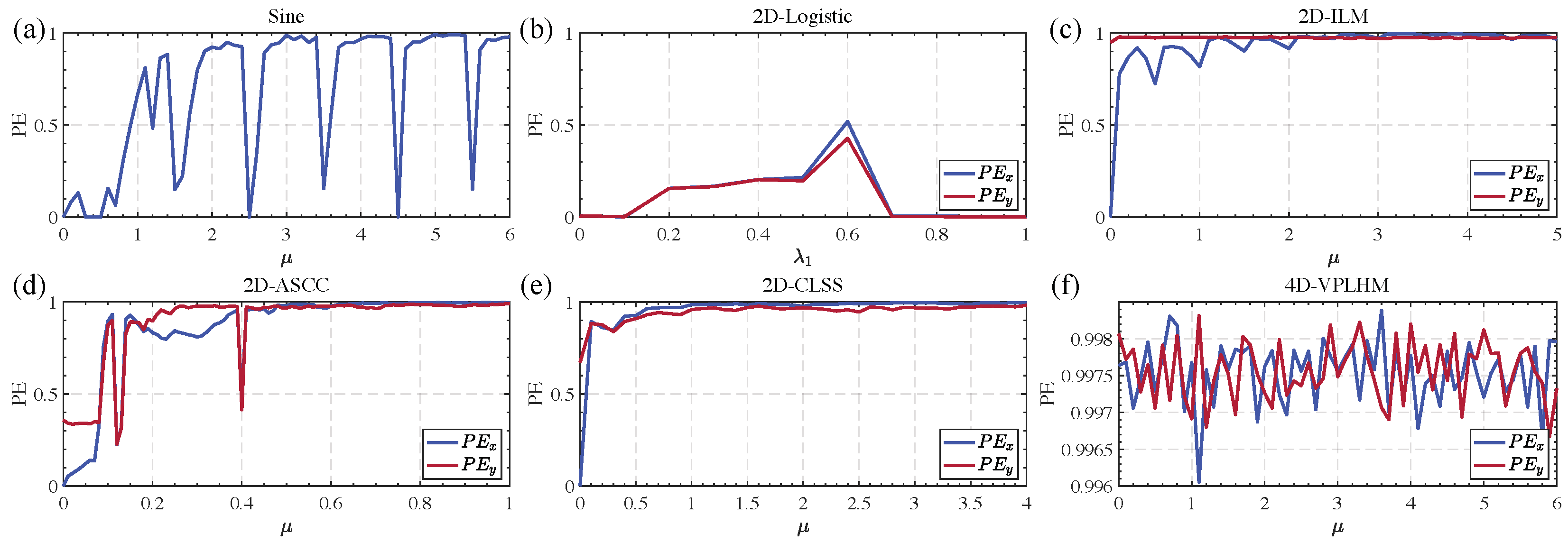
Figure 5.
Comparison results of permutation entropy: (a) Sine chaotic system, (b) 2D-Logistic chaotic system, (c) 2D-ILM chaotic system, (d) 2D-ASCC chaotic system, (e) 2D-ClSS chaotic system, (f) 4D-VPLHM chaotic system.
Figure 5.
Comparison results of permutation entropy: (a) Sine chaotic system, (b) 2D-Logistic chaotic system, (c) 2D-ILM chaotic system, (d) 2D-ASCC chaotic system, (e) 2D-ClSS chaotic system, (f) 4D-VPLHM chaotic system.
Figure 6.
Flowchart of the encryption scheme.
Figure 6.
Flowchart of the encryption scheme.
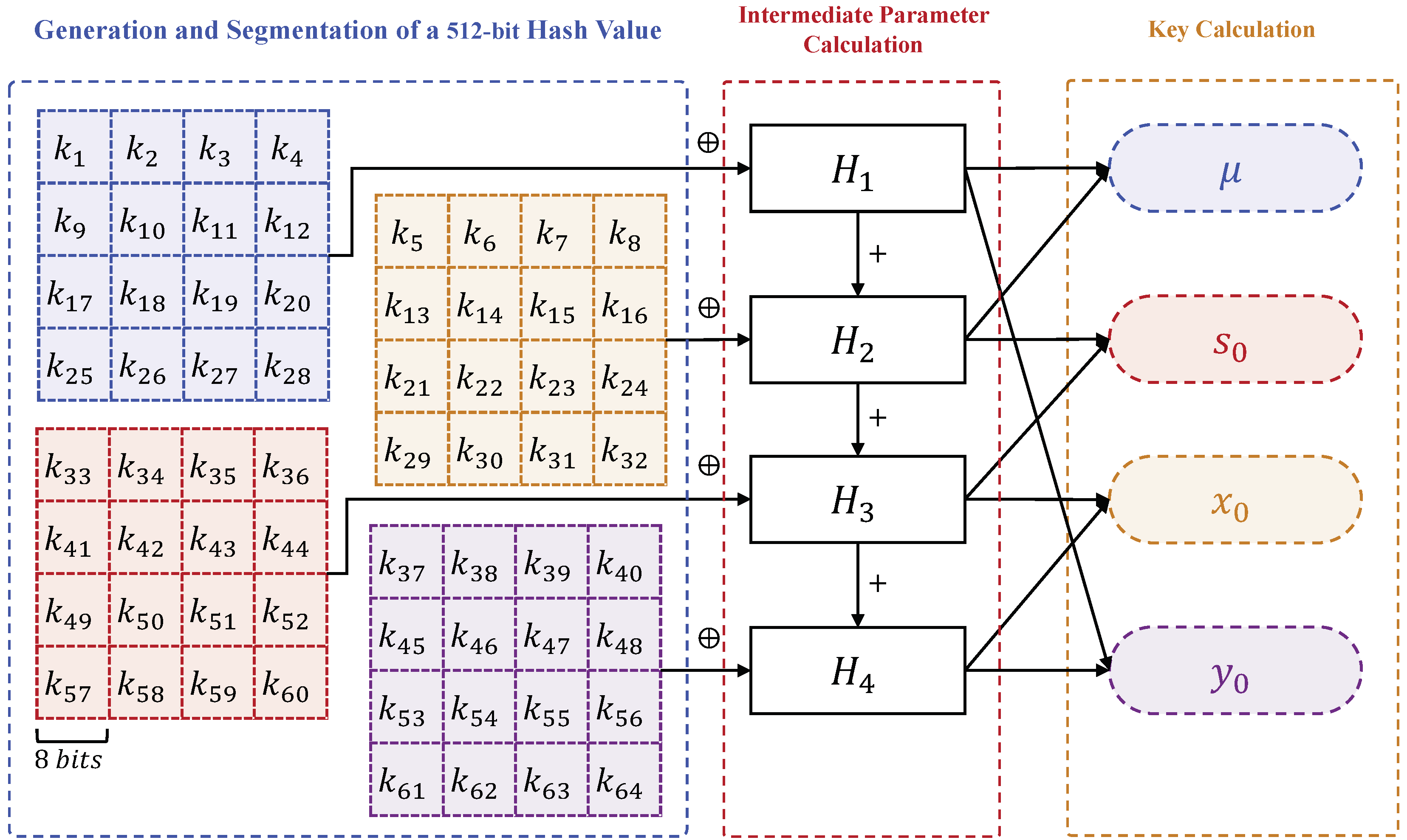
Figure 7.
Flowchart of key generation algorithm.
Figure 7.
Flowchart of key generation algorithm.
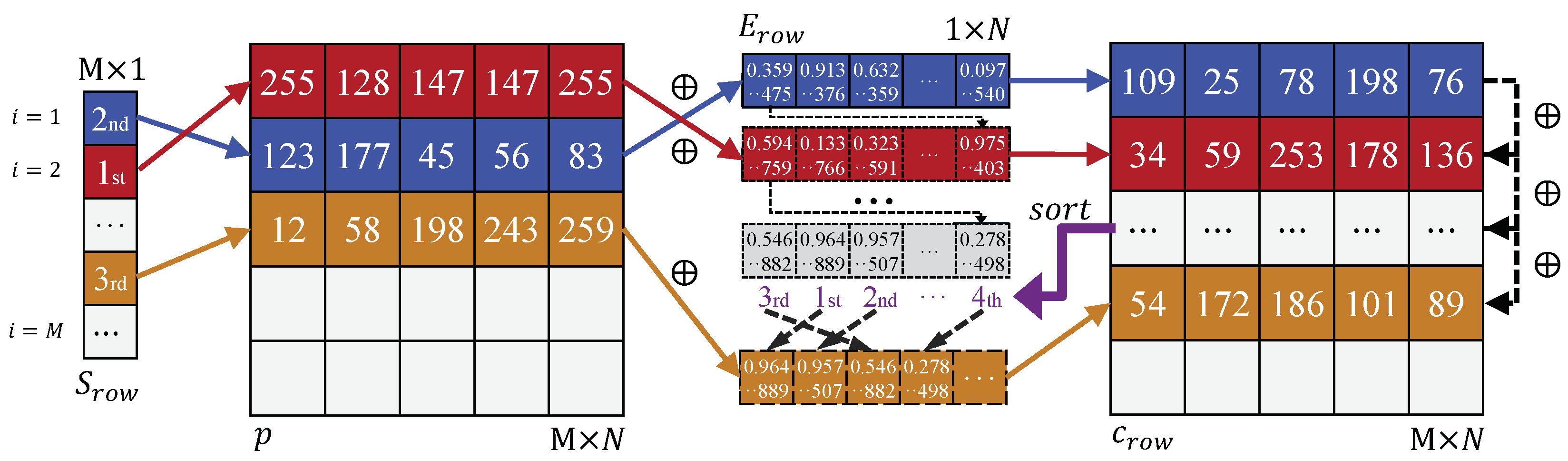
Figure 8.
Example of row scrambling and diffusion encryption procedures.
Figure 8.
Example of row scrambling and diffusion encryption procedures.
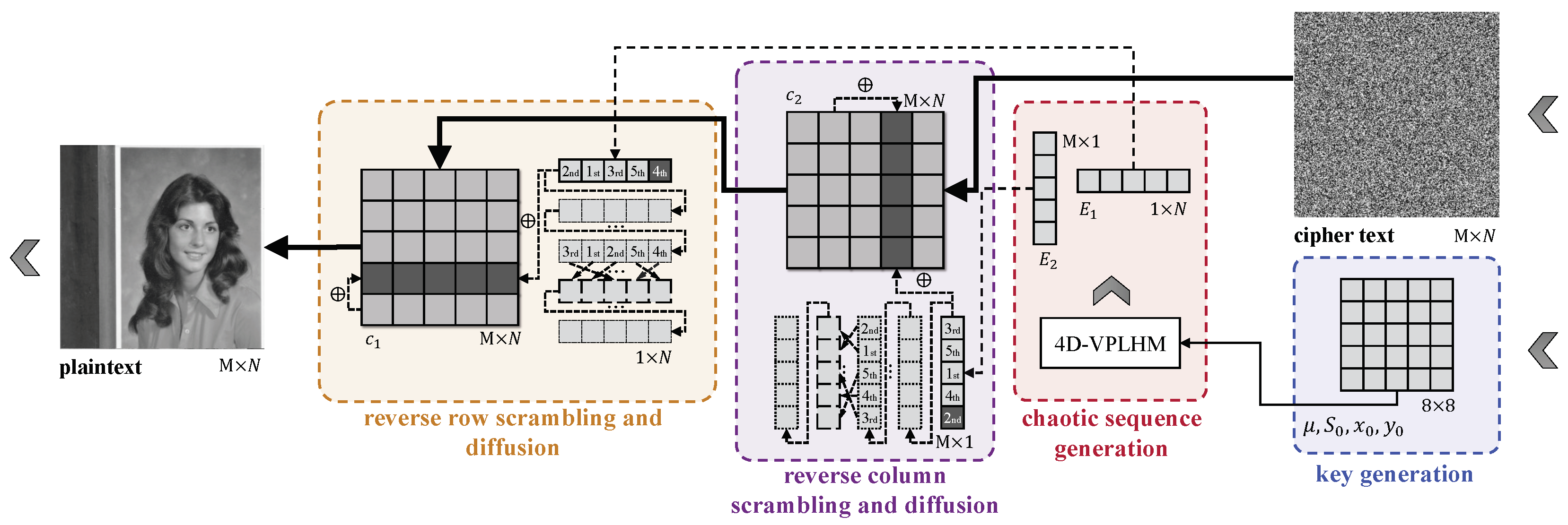
Figure 9.
Decryption scheme flowchart.
Figure 9.
Decryption scheme flowchart.
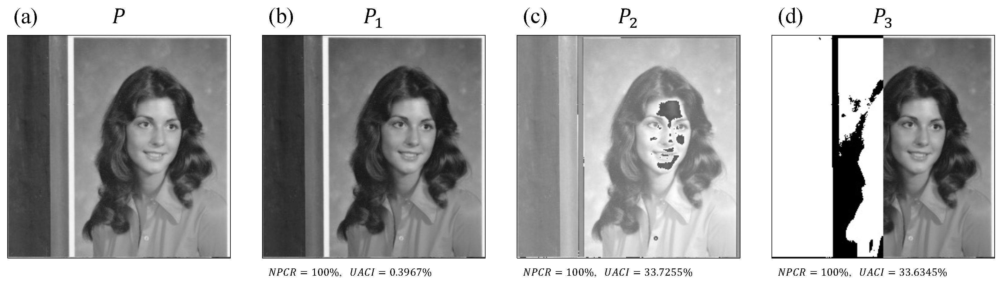
Figure 10.
Images constructed based on the original Female image. (a) The original Female image. (b) Constructed image , obtained by adding 1 to each pixel value of the original image. (c) Resultant image , obtained by applying a pixel difference of 85 to every pixel value of the original image. (d) Resultant image , obtained by inverting half of the pixels of the original image and applying a pixel difference of 1 to the remaining half.
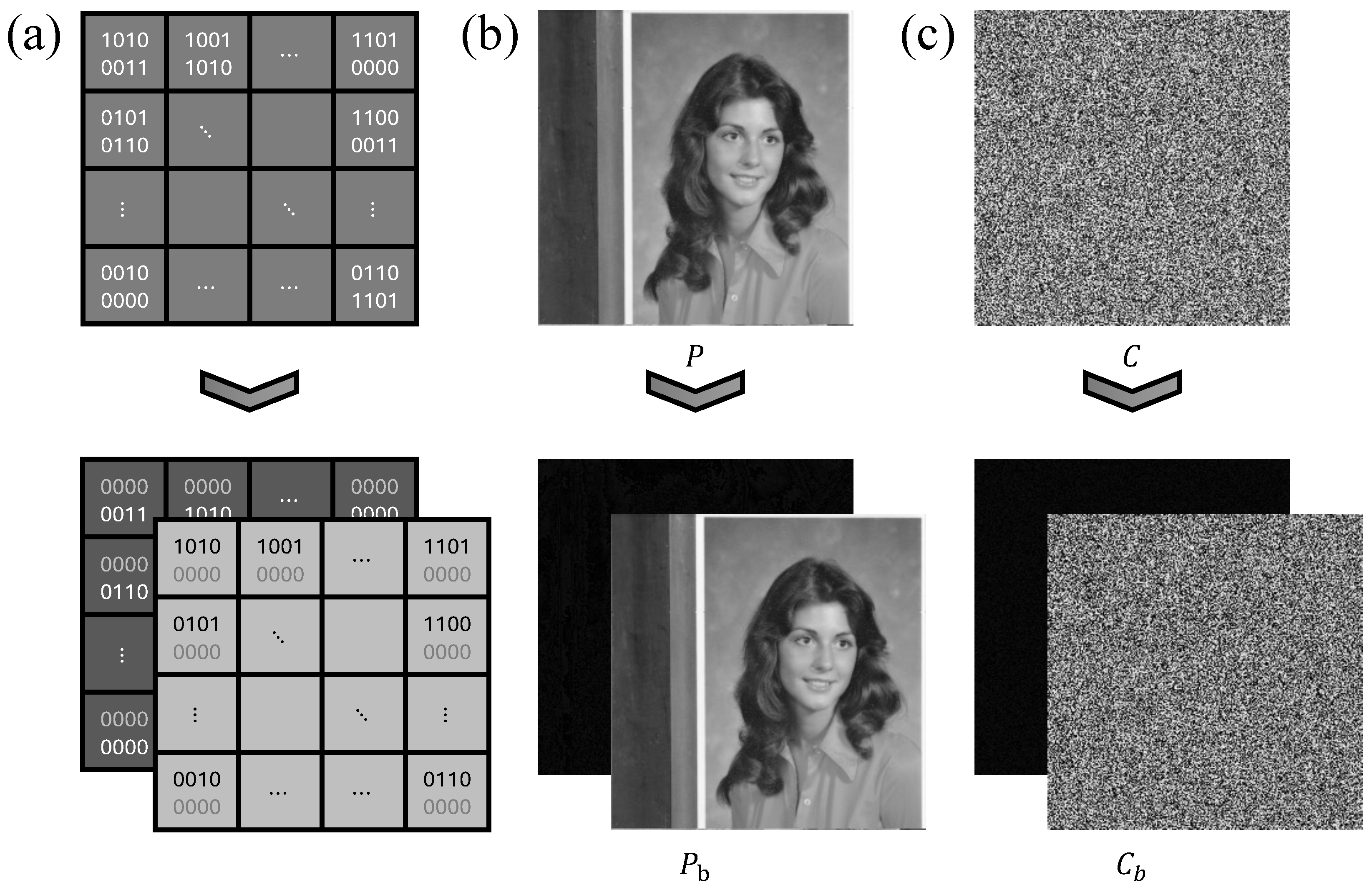
Figure 11.
Binary partition example. (a) Example of pixel value bit-plane decomposition. (b) Bit-plane decomposition of Female pixel values. (c) Bit-plane decomposition of pixel values in random pixel maps.
Figure 11.
Binary partition example. (a) Example of pixel value bit-plane decomposition. (b) Bit-plane decomposition of Female pixel values. (c) Bit-plane decomposition of pixel values in random pixel maps.
Figure 12.
Encryption and decryption simulation results. (a–e) Original images of Female, Boat, Gray, Text, and X-ray, respectively. (f–j) Encrypted images of Female, Boat, Gray, Text, and X-ray, respectively. (k–o) Decrypted images of Female, Boat, Gray, Text, and X-ray, respectively.
Figure 12.
Encryption and decryption simulation results. (a–e) Original images of Female, Boat, Gray, Text, and X-ray, respectively. (f–j) Encrypted images of Female, Boat, Gray, Text, and X-ray, respectively. (k–o) Decrypted images of Female, Boat, Gray, Text, and X-ray, respectively.
Figure 13.
Female figure key sensitivity test results. (a–h), respectively, shows the , , , , , , , position decryption result after key change.
Figure 13.
Female figure key sensitivity test results. (a–h), respectively, shows the , , , , , , , position decryption result after key change.
Figure 14.
Histogram analysis results for test images before and after encryption. (a–e) represent the histograms of the original images for Female, Boat, Gray, Text, and X-ray, respectively. (f–j) represent the histograms of the encrypted images for Female, Boat, Gray, Text, and X-ray, respectively.
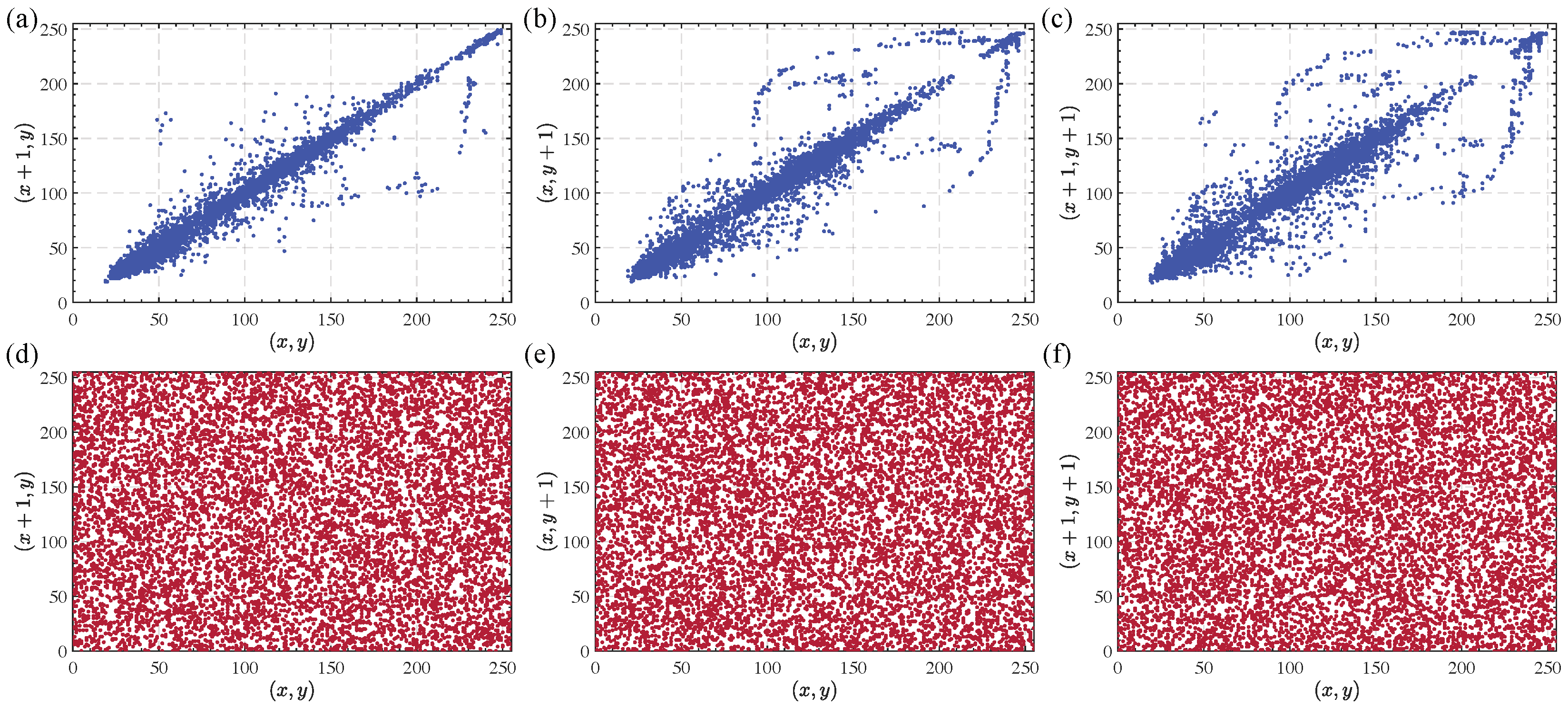
Figure 15.
Adjacent pixel distribution of the Female image before and after encryption. (a–c) depict the distributions of adjacent pixels in the horizontal, vertical, and diagonal directions for the original Female image. (d–f) illustrate the corresponding distributions for the encrypted Female image.
Figure 16.
Comparison of image encryption time for different sizes.
Figure 16.
Comparison of image encryption time for different sizes.
Table 1.
NIST randomness test results for 4D-VPLHM.
Table 1.
NIST randomness test results for 4D-VPLHM.
| Statistical Test | Proportion (%) | p-Value | Result |
|---|
| X
| Y
| X
| Y
| X | Y |
|---|
| Frequency | 98.60 | 98.80 | 0.7090 | 0.5958 | Pass | Pass |
| BlockFrequency | 99.20 | 98.60 | 0.6188 | 0.2819 | Pass | Pass |
| CumulativeSums | 98.70 | 99.00 | 0.4152 | 0.5557 | Pass | Pass |
| Runs | 99.20 | 99.20 | 0.5572 | 0.5583 | Pass | Pass |
| LongestRun | 98.90 | 98.20 | 0.3861 | 0.5634 | Pass | Pass |
| Rank | 98.60 | 98.80 | 0.2963 | 0.6549 | Pass | Pass |
| FFT | 99.40 | 99.80 | 0.5479 | 0.5751 | Pass | Pass |
| NonOverlappingTemplate | 99.03 | 99.00 | 0.5043 | 0.4905 | Pass | Pass |
| OverlappingTemplate | 98.40 | 98.80 | 0.5089 | 0.5792 | Pass | Pass |
| Universal | 98.80 | 98.60 | 0.6656 | 0.3543 | Pass | Pass |
| ApproximateEntropy | 99.00 | 98.60 | 0.3831 | 0.6586 | Pass | Pass |
| RandomExcursions | 98.80 | 99.03 | 0.4347 | 0.3668 | Pass | Pass |
| RandomExcursionsVariant | 99.36 | 99.05 | 0.4516 | 0.3889 | Pass | Pass |
| Serial | 99.40 | 99.00 | 0.4892 | 0.6142 | Pass | Pass |
| LinearComplexity | 98.40 | 98.40 | 0.7400 | 0.4620 | Pass | Pass |
Table 2.
TestU01 randomness test results for six chaotic systems.
Table 2.
TestU01 randomness test results for six chaotic systems.
| Chaos | Alphabit Test | BlockAlphabit Test | Alphabit Test |
|---|
| X
| Y
| X
| Y
| X
| Y
|
|---|
| Sine | 0/17 | - | 0/102 | - | 34/39 | - |
| 2D-Logistic | 0/17 | 0/17 | 0/102 | 0/102 | 0/39 | 0/39 |
| 2D-ILM | 17/17 | 3/17 | 101/102 | 15/102 | 39/39 | 8/39 |
| 2D-CLSS | 0/17 | 4/17 | 0/102 | 39/102 | 4/39 | 25/39 |
| 2D-ACSS | 0/17 | 4/17 | 3/102 | 13/102 | 5/39 | 10/39 |
| 4D-VPLHM | 17/17 | 17/17 | 102/102 | 101/102 | 39/39 | 39/39 |
Table 3.
The percentage of information content carried by different bits.
Table 3.
The percentage of information content carried by different bits.
| Bit Index | 1 | 2 | 3 | 4 | 5 | 6 | 7 | 8 |
| Percentage (%) | 0.3922 | 0.7843 | 1.5686 | 3.1373 | 6.2745 | 12.5490 | 25.0980 | 50.1961 |
Table 4.
BL-NPCR and BL-UACI calculation results for Female image.
Table 4.
BL-NPCR and BL-UACI calculation results for Female image.
| Image | NPCR (%) | UACI (%) | BL-NPCR (%) | BL-UACI (%) |
|---|
| P vs. | 100 | 0.3967 | 0.8667 | 0.4096 |
| P vs. | 100 | 33.7255 | 6.8314 | 29.8235 |
| P vs. | 100 | 32.6345 | 0.4715 | 27.3170 |
Table 5.
NIST randomness test results of the cyclic shift algorithm.
Table 5.
NIST randomness test results of the cyclic shift algorithm.
| Statistical Test | Proportion (%) | P-Value | Result |
|---|
| x
| y
| z
| x
| y
| z
| x
| y
| z
|
|---|
| Frequency | 98.60 | 98.80 | 100.00 | 0.7090 | 0.6523 | 0.0000 | Pass | Pass | fail |
| BlockFrequency | 99.20 | 98.40 | 100.00 | 0.6188 | 0.5106 | 0.0554 | Pass | Pass | Pass |
| CumulativeSums | 98.70 | 98.50 | 100.00 | 0.4152 | 0.2949 | 0.0000 | Pass | Pass | fail |
| Runs | 99.20 | 99.20 | 100.00 | 0.5572 | 0.4227 | 0.0000 | Pass | Pass | fail |
| LongestRun | 98.90 | 99.20 | 100.00 | 0.3861 | 0.6572 | 0.0000 | Pass | Pass | fail |
| Rank | 98.60 | 99.40 | 100.00 | 0.2963 | 0.1463 | 0.0000 | Pass | Pass | fail |
| FFT | 99.40 | 99.20 | 99.00 | 0.5479 | 0.3060 | 0.1719 | Pass | Pass | Pass |
| NonOverlappingTemplate | 99.03 | 98.98 | 100.00 | 0.5043 | 0.5150 | 0.0000 | Pass | Pass | fail |
| OverlappingTemplate | 98.40 | 98.60 | 100.00 | 0.5089 | 0.6960 | 0.0000 | Pass | Pass | fail |
| Universal | 98.80 | 97.80 | 100.00 | 0.6656 | 0.4701 | 0.0067 | Pass | Pass | fail |
| ApproximateEntropy | 99.00 | 98.20 | 100.00 | 0.3831 | 0.5179 | 0.0000 | Pass | Pass | fail |
| RandomExcursions | 98.80 | 98.84 | 100.00 | 0.4347 | 0.4151 | 0.0040 | Pass | Pass | fail |
| RandomExcursionsVariant | 99.36 | 99.16 | 100.00 | 0.4516 | 0.3662 | 0.0669 | Pass | Pass | Pass |
| Serial | 99.40 | 98.30 | 93.00 | 0.4892 | 0.6239 | 0.0000 | Pass | Pass | fail |
| LinearComplexity | 98.40 | 99.20 | 100.00 | 0.7400 | 0.4464 | 0.0000 | Pass | Pass | fail |
Table 6.
TestU01 randomness test results and time consumption comparison of the cyclic shift algorithm.
Table 6.
TestU01 randomness test results and time consumption comparison of the cyclic shift algorithm.
| Results | TestU01 | Time (s) |
|---|
| Alphabit Test
| BlockAlphabit Test | Alphabit Test |
|---|
| x | 17/17 | 102/102 | 39/39 | 1.6016 ± 0.0228 |
| y | 17/17 | 99/102 | 37/39 | 0.0863 ± 0.0127 |
| z | 1/17 | 0/102 | 0/39 | 0.0545 ± 0.0023 |
Table 7.
Information entropy test results.
Table 7.
Information entropy test results.
| Image | Female | Boat | X-Ray | Text | Gray | Lena | SIMP |
|---|
| Plain | 7.1325 | 7.2361 | 7.5574 | 5.2645 | 5.4029 | 7.5150 | 6.6121 |
| Ciphertext | 7.9992 | 7.9991 | 7.9992 | 7.9994 | 7.9992 | 7.9993 | 7.9993 |
Table 8.
Information entropy comparison results for the Lena image.
Table 8.
Information entropy comparison results for the Lena image.
| Algorithm | Ref. [28] | Ref. [29] | Ref. [30] | Ref. [31] | Ref. [32] | Ref. [33] | Ours |
|---|
| Information entropy | 7.9974 | 7.9560 | 7.9977 | 7.9971 | 7.9992 | 7.9972 | 7.9993 |
Table 9.
Adjacent pixel correlation results before and after encryption of the test image.
Table 9.
Adjacent pixel correlation results before and after encryption of the test image.
| Image | Plaintext | Ciphertext |
|---|
| Horizontal
| Vertical
| Diagonal
| Horizontal
| Vertical
| Diagonal
|
|---|
| Female | 0.9846 | 0.9694 | 0.9556 | 0.0016 | 0.0103 | 0.0029 |
| Boat | 0.9233 | 0.8865 | 0.8353 | 0.0029 | −0.0144 | −0.0106 |
| X-Ray | 0.9919 | 0.9866 | 0.9798 | 0.0017 | −0.0015 | −0.0018 |
| Text | 0.7098 | 0.7835 | 0.4811 | −0.0001 | 0.0061 | 0.0014 |
| Gray | 0.9997 | 0.9942 | 0.9944 | 0.0022 | 0.0106 | −0.0040 |
| Lena | 0.9556 | 0.9190 | 0.8816 | −0.0015 | 0.0024 | −0.0011 |
| SIMP | 0.8594 | 0.8494 | 0.7514 | −0.0029 | −0.0014 | 0.0001 |
Table 10.
Comparison of adjacent pixel correlation after encryption of Lena image using different algorithms.
Table 10.
Comparison of adjacent pixel correlation after encryption of Lena image using different algorithms.
| Direction | Ref. [28] | Ref. [34] | Ref. [35] | Ref. [36] | Ref. [37] | Ours |
|---|
| Horizontal | −0.0158 | −0.0030 | 0.0075 | 0.0021 | 0.0026 | −0.0015 |
| Vertical | −0.0118 | −0.0034 | −0.0031 | 0.0099 | 0.0032 | 0.0024 |
| Diagonal | 0.0004 | 0.0099 | 0.0016 | 0.0011 | 0.0057 | −0.0011 |
Table 11.
Differential analysis results of test images.
Table 11.
Differential analysis results of test images.
| Image | NPCR (%) | UACI (%) | BL-UACI (%) | BL-UACI (%) |
|---|
| Female | 99.6074 (−0.0020) | 33.4564 (−0.0071) | 93.7463 (−0.0037) | 35.4083 (−0.0084) |
| Boat | 99.6082 (−0.0012) | 33.4607 (−0.0028) | 93.7394 (−0.0106) | 35.4106 (−0.0061) |
| X-ray | 99.6103 (+0.0009) | 33.4543 (−0.0092) | 93.7464 (−0.0036) | 35.4074 (−0.0093) |
| Text | 99.6112 (+0.0018) | 33.4311 (−0.0324) | 93.7533 (+0.0033) | 35.3809 (−0.0358) |
| Gray | 99.6117 (+0.0023) | 33.5217 (+0.0582) | 93.7551 (+0.0051) | 35.4784 (+0.0617) |
| Lena | 99.6076 (−0.0018) | 33.4817 (+0.0182) | 93.7590 (+0.0090) | 35.4333 (+0.0166) |
| SIMP | 99.6092 (−0.0002) | 33.4611 (−0.0024) | 93.7492 (−0.0008) | 35.4119 (−0.0048) |
Table 12.
Comparison of differential analysis results of different algorithms on the Lena image.
Table 12.
Comparison of differential analysis results of different algorithms on the Lena image.
| Algorithm | NPCR (%) | UACI (%) | BL-UACI (%) | BL-UACI (%) |
|---|
| Ref. [38] | 99.6026 (+0.0068) | 30.3008 (+3.1629) | 93.7268 (+0.0232) | 32.3934 (+2.0233) |
| Ref. [39] | 99.5792 (+0.0302) | 33.4532 (+0.0103) | 93.7291 (+0.0209) | 35.3867 (+0.0300) |
| Ref. [40] | 99.5697 (+0.0397) | 33.4100 (+0.0535) | 93.6970 (+0.0530) | 35.3270 (+0.0879) |
| Ref. [41] | 99.6210 (+0.0116) | 33.4750 (+0.0115) | 93.6434 (+0.1066) | 35.2921 (+0.1246) |
| Ref. [42] | 99.6006 (+0.0088) | 34.6379 (+1.1744) | 93.5217 (+0.2283) | 33.8523 (+1.5644) |
| Ours | 99.6076 (−0.0018) | 33.4817 (+0.0182) | 93.7590 (+0.0090) | 35.4333 (+0.0166) |
Table 13.
Encryption algorithm efficiency analysis results.
Table 13.
Encryption algorithm efficiency analysis results.
| Algorithm | Encryption Time (s) | ET (256 × 256) | NCPB (256 × 256) |
|---|
| 256 × 256 | 512 × 512 | 1024 × 1024 |
|---|
| Ref. [43] | 0.0794 | 0.3062 | 1.41705 | 0.7871 | 3150.0244 |
| Ref. [44] | 0.2860 | 1.3640 | 3.5440 | 0.2180 | 11,346.4355 |
| Ref. [45] | 0.0318 | 0.1284 | 0.5345 | 1.9654 | 1261.5966 |
| Ref. [46] | 0.0625 | 0.2500 | 0.9845 | 1 | 2479.5532 |
| Ref. [47] | 0.0323 | 0.1536 | 0.7109 | 1.9349 | 1281.4331 |
| Ours | 0.0246 | 0.0618 | 0.2231 | 2.5406 | 975.9521 |


