Abstract
Standard correlation analysis is one of the frequently used methods in financial markets. However, this matrix can give erroneous results in the conditions of chaos, fractional systems, entropy, and complexity for the variables. In this study, we employed the time-dependent correlation matrix based on isospectral flow using the Lie group method to assess the price of Bitcoin and gold from 19 July 2010 to 31 December 2024. Firstly, we showed that the variables have a chaotic and fractional structure. Lo’s rescaled range (R/S) and the Mandelbrot–Wallis method were used to determine fractionality and long-term dependence. We estimated and tested the d parameter using GPH and Phillips’ estimators. Renyi, Shannon, Tsallis, and HCT tests determined entropy. The KSC determined the evidence of the complexity of the variables. Hurst exponents determined mean reversion, chaos, and Brownian motion. Largest Lyapunov and Hurst exponents and entropy methods and KSC found evidence of chaos, mean reversion, Brownian motion, entropy, and complexity. The BDS test determined nonlinearity, and later, the time-dependent correlation matrix was obtained by using the stochastic SO(2) Lie group. Finally, we obtained robustness check results. Our results showed that the time-dependent correlation matrix obtained by using the stochastic SO(2) Lie group method yielded more successful results than the ordinary correlation and covariance matrix and the Spearman correlation and covariance matrix. If policymakers, financial managers, risk managers, etc., use the standard correlation method for economy or financial policies, risk management, and financial decisions, the effects of nonlinearity, fractionality, entropy, and chaotic structures may not be fully evaluated or measured. In such cases, this can lead to erroneous investment decisions, bad portfolio decisions, and wrong policy recommendations.
Keywords:
correlation flow; covariance flow; stochastic SO(2) Lie method; fractal; chaos; Bitcoin gold MSC:
00A69; 22E60; 62P20
1. Introduction
In mathematical finance, various researchers have used the Lie technique to obtain insight into linked partial differential equations. The use of differentiable manifolds for interest rate models was investigated in papers [1,2,3]. Reference [2] used the Lie technique to solve the BSM equation, whereas Reference [4] and Reference [5] presented a short rate model depending on the manifold . Short-term interest rate models for and manifolds were built utilizing matrix representations of Lie groups, which is the standard approach [6]. Reference [7] used the Lie method to analyze interest rate. Furthermore, Reference [8] used Lie–LSTMOLS methods to investigate oil price volatility.
On the other hand, some papers used a Lie correlation matrix. A correlation matrix should satisfy the following properties:
i. The diagonal elements of a correlation matrix are always equal to one, while the absolute values of the non-diagonal elements do not exceed one.
ii. Correlation matrices are positive semi-definite and real symmetric, which means that none of the eigenvalues are negative. The authors of Reference [9] employed the Lie approach for their correlation matrix. Correlation matrices are used extensively in risk management and finance, among other applications.
The purpose of this study is to use real market data to create correlation flows that satisfy the requirements listed above and approach the valid correlation. There are existing solutions available to address the same problem; see [10,11,12,13].
Newton-based approaches for approximating covariance matrices are described in [14,15,16]. Furthermore, there are approaches that use hyper-spherical decomposition [17] and unconstrained convex optimization [18]. However, at least one of the desired characteristics of a correlation matrix described above is lacking in several techniques. In particular, positive semi-definiteness is a criterion that is poorly implemented. For example, the strategy described in [19] has problems in other areas of the matrix in order to maintain positive semi-definiteness. Reference [20] proposed a method to obtain the time-dependent correlation matrix based on isospectral flow, and in this proposal, only an initial correlation matrix is needed, and they applied the SVD method for solution. Reference [9] solved the stochastic differential equation expressed with special orthogonal groups and algebras to obtain the correlation flow. They used real market data to construct a correlation flow that fulfills the aforementioned criteria and approaches the valid correlation.
However, these papers do not explore evidence of chaotic structures, whereas in real life, the variables can exhibit often chaotic and fractional structures, entropy, and complexity. For example, there are studies in many different fields with these types of variables [21,22]. For this reason, in our study, we employed the time-dependent correlation matrix based on isospectral flow using the Lie group method, and we aimed to construct a time-dependent correlation matrix using this method for variables that exhibit a chaotic structure. This article investigates the period from 19 July 2010 to 31 December 2024, addressing daily events, including major events, affecting Bitcoin and gold prices. Economic and non-economic factors such as war, military operations, and pandemics are examples of unavoidable challenges. These events can affect the nonlinearity, chaotic and fractal structures, entropy, and complexity states of Bitcoin and gold prices, thereby emphasizing the importance of modeling dynamic phenomena and addressing SDEs. Within the scope of our study, we first investigated the chaotic and fractal structure of the variables we used. For this, we applied Lo’s rescaled range (R/S) and the Mandelbrot–Wallis method to determine fractionality and long-term dependence. The d parameter using GPH and Phillips’ estimators was applied. Renyi, Shannon, Tsallis, and HCT entropy tests were employed to determine entropy. The Kolmogorov–Sinai complexity (KSCM) method determined the evidence of the complexity of the variables. Hurst exponents were employed to explore the evidence of mean reversion, chaos, and Brownian motion. Largest Lyapunov exponents (LLEs) were used to explore the evidence of chaos. Then, the time-dependent correlation matrix, obtained by using the stochastic SO(2) Lie group, was employed. Finally, we conducted a robustness check. We will compare the results obtained from the stochastic SO(2) Lie group method and standard method.
2. Mathematical Method
Analytic Method for Stochastic SO(2) Lie Method
It is known that the Lie group is a geometrically differentiable manifold, and its algebra is a vector space tangent to the manifold at unit. Therefore, the stochastic differential equation is obtained by using the relation between the SO(2) Lie group and its algebra for covariance flows. The numerical solution of this equation is explained in the experimental method section [23,24].
and
A typical element of is given by the matrix , and the manifold of this group is expressed by the parametrization , . The transformation between these two algebraic structures is as follows:
and
To obtain time-dependent correlation matrices, first, the covariance flow is defined as follows:
where
are the time-dependent covariance matrices of the covariance space
, and is the initial covariance matrix.
Based on the definitions given above, stochastic differential equations based on the Lie group are given as follows:
where is an orthogonal matrix, while and represent standard Brownian motion. As explained above, geometrically, the Lie group SO(2) is a differentiable manifold, and the Lie algebra SO(2) has the structure of a tangent vector space to the manifold. Therefore, the Lie group has a global structure, while the Lie algebra has a local structure. It is usually easier and more convenient to work in the local structure. Therefore, to solve SDE (4), SDE (5) is given by the Magnus expansion using the relation between the group and the algebra. Detailed proof can be found in Theorem 5 of [25].
where
, and represents Bernoulli numbers; the adjoint operator has the following properties:
Thus, SDE (5) is implemented in the Lie algebra (space) SO(2) of 2 × 2 anti-symmetric matrices. For the solution of SDE (4), the results derived using the geometric Euler–Maruyama scheme are given in detail on page 7.
For the stochastic Lie method, the convergence of the solution is given by the geometric Euler–Maruyama scheme, which preserves the geometric of the Lie group SO(2). The geometric Euler–Maruyama scheme converges with rate with respect to the mean uniform squared error over the whole interval [0, T] (for detailed information, see [24]). As a result, the correlation matrices are defined by the following equation:
3. Data and Experimental Results
3.1. Data
In this study, we used a historical dataset that consists of daily Bitcoin (BTC) and gold (XAU). The sample period was 19 July 2010–31 December 2024. After 2012, BTC was accepted in financial markets, and BTC transactions and volume increased significantly in both global financial markets and cryptocurrency markets; furthermore, there was a great halving event for Bitcoin in 2012. Although the price movements after 2012 were more important in Bitcoin prices, there was no period restriction. This is an important point to show the differentiation from the standard method. XAU is the price of gold. Gold has always been an important financial instrument and a safe investment instrument. Gold and Bitcoin can be accepted as stores of value and inflation hedges, but Bitcoin is far more volatile and speculative than gold. Their relation is sometimes positively correlated, especially during macroeconomic stress, but not always. Investors often employ both to hedge against fiat currency risks, though they exhibit different characters in most portfolios. To determine the correlation and covariance between these two is important in this sense.
The variables were not of the same frequency. Therefore, all variables were brought to the same frequency. The weekend was causing frequency differences, especially among the variables. At this stage, data were not obtained by automatically determining the period by setting it up from Phyton or other programs. Individual data were analyzed and harmonized. In cases where there were no data for two variables for the same day, they were excluded from the analysis on that day. So, a common date was determined for the two variables.
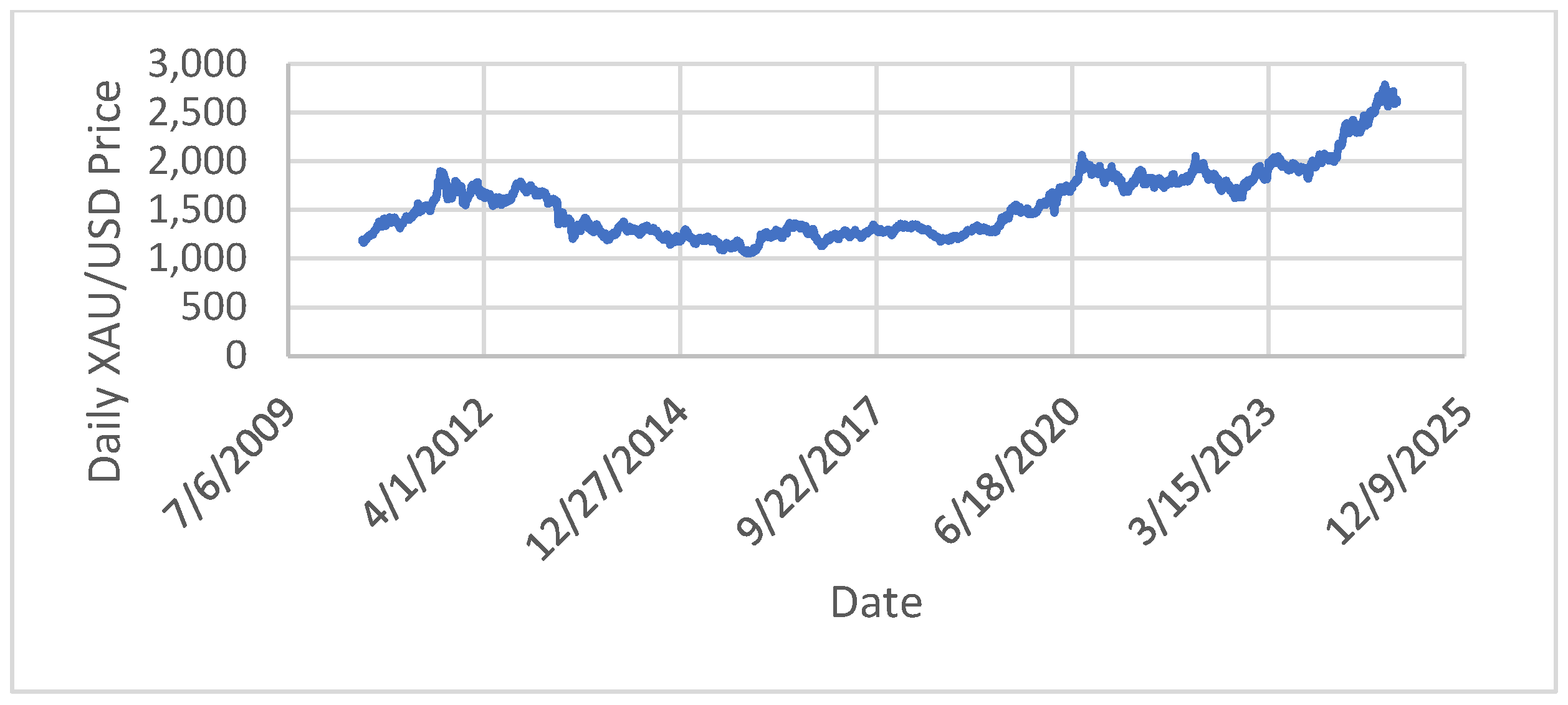
Figure 1 and Figure 2 show the daily BTC and XAU prices for the examined time period. The overviews suggest that all variables are subject to volatility clustering. The BTC and XAU variables are also subject to strong outliers in certain periods.
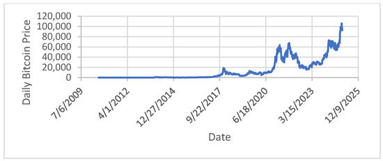
Figure 1.
Daily BTC price from 19 July 2010 to 31 December 2024. Source: https://tr.investing.com/crypto/bitcoin/historical-data (accessed on 7 January 2025).
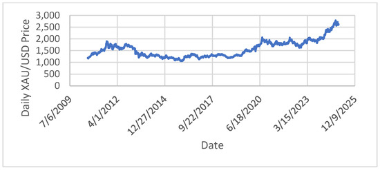
Figure 2.
Daily XAU/USD price from 19 July 2010 to 31 December 2024. Source: https://tr.investing.com/currencies/xau-usd-historical-data (accessed on 7 January 2025).
In this study, the level series and the first difference series were used to determine nonlinearity and other structures. The first difference was determined as series BTCt/BTCt-1 and XAUt/XAUt-1.
In Table 1, for level and first-differenced series, the results of descriptive statistics are shown. In terms of Bitcoin and XAU prices and their variability for the different series, the skewness statistics also indicate strong skewness, with there being negative values for BTC and positive values for XAU. The results show high kurtosis statistics. The JB test rejects the null of normality at conventional levels for both variables. BTC and XAU do not follow normal distributions.

Table 1.
Descriptive statistics.
Table 1’s findings are consistent with Figure 1 and Figure 2, which provide insights into the series’ excess kurtosis, possible nonlinearity, volatility clustering, and asymmetry. These findings are supported by the JB test results, excess kurtosis, and skewed distributions, all of which indicate that the series under consideration is not normal.
3.2. Empirical Stage
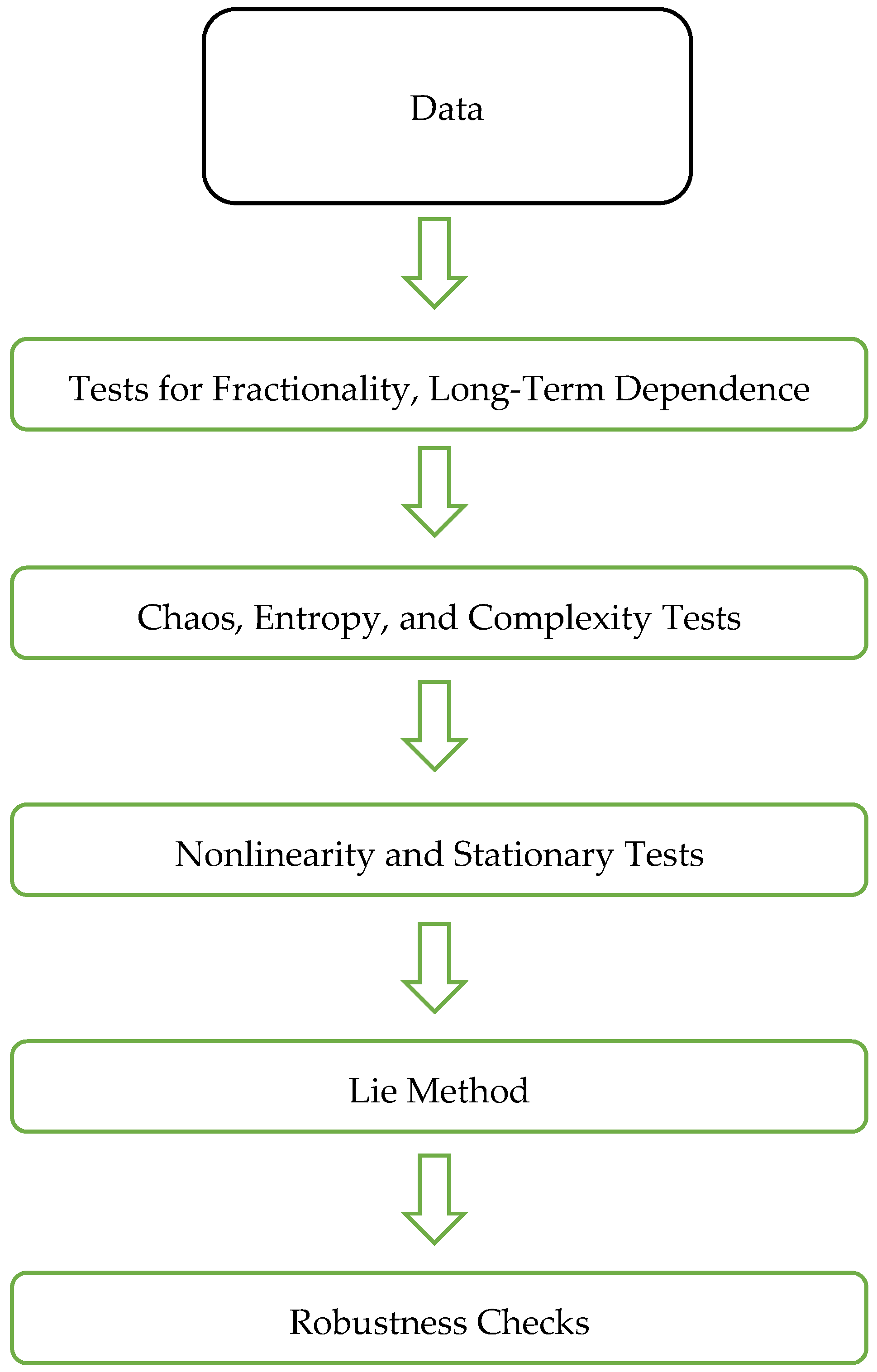
Empirical results were obtained in all five stages. Different package programs were used to obtain the results. MATLAB-R2024b, Python-3.12.1, Stata-17, and EViews-12 are among these programs. The flow chart in Figure 3 shows these stages.
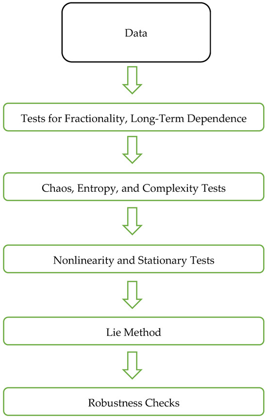
Figure 3.
Flow chart.
We considered the following five steps:
- i.
- Fractionality and Long-term Dependence (LtD): LtD was analyzed using fractional difference parameters and two R/S tests. The tests are proven, robust methods for autocorrelation and heteroskedasticity. These tests were conducted as follows:
- ○
- We used Lo’s R/S test [26] and the Hurst–Mandelbrot R/S test [27,28,29] for long-run dependence.
- ○
- The d parameter was estimated and tested with GPH [30] and Phillips’ estimators [31].
- ii.
- Chaotic Dynamics, Entropy, LLE, and Complexity.
- ○
- Rényi [32], Shannon [33], and Tsallis [34] entropy that generalizes HCT [35] tests were employed to determine entropy.
- ○
- The KSC test was employed to determine the evidence of complexity of the variables.
- ○
- The evidence of mean-reversion, chaos, and Brownian motion was determined by Hurst exponents [27].
- ○
- The LLE (λ) was computed.
The λ results indicate the following:
- ■
- λ > 0 specifies chaos; λ > 1 indicates deterministic chaos.
If 0 < λ < 1, and the KSCM and the entropies determined a positive value, the results propose an acceptable degree of random processes or uncertainty.
- iii.
- Nonlinearity Testing.
- ○
- We used the BDS test [36] for nonlinearity and independence.
- ○
- The stationarity of the variables was examined using the nonlinear unit root test proposed by KSS [37].
- iv.
- Modeling of the Lie Method
The Lie method involves approximating correlation matrices through the following steps:
- 1.
- Estimation of the Density Function: The risk manager estimates the density function of the correlation using historical data. This serves as a reference for the stochastic behavior of correlations over time.
- 2.
- Generation of Time-Dependent Correlation Matrices: The goal is to construct correlation matrices that are not only valid but also reflect the time-varying and stochastic nature of correlations. These matrices should align with the estimated density function from historical data.
- 3.
- Alignment with Historical Data: The constructed correlation matrices are designed to match the density function for the historical data, ensuring that the stochastic correlations are consistent with observed market behavior.
- 4.
- The numerical solution scheme of the time-dependent correlation matrices defined in the analytical method using the Stochastic SO(2) Lie group method is given as follows:
- ○
- Using Equation (5), obtained by the Magnus expansion (proof of which is given in detail in Theorem 5 [25]), the flow stages for the numerical solution of Equation (4) are given as follows:Step 1: The interval [0, T] is divided into n sub-intervals [ti, ti+1], .Step 2: The following steps are repeated with the beginning t0 = 0 and A0 = A(0) = I.Step 3: Let the approximations of , at be , , respectively.Step 4: For the geometric Euler–Maruyama scheme,Step 5: Set .
- ○
- The orthogonal matrix is found such that , where is the initial covariance matrix. Here, D is the diagonal matrix consisting of the eigenvalues of C.
- ○
- After obtaining the covariance flow , the correlation flow
was obtained as .
- v.
- Robustness Check
The results determined by the Lie method will be compared with the results of the standard method.
3.3. Experimental Results
3.3.1. Long-Term Dependence and Fractionality
Lo’s R/S test [27] and the Hurst–Mandelbrot R/S test [28,29,30] were used to assess the series for long memory. Table 2 shows the results.
Table 2.
Estimation results.
For all variables that are listed in Table 2, the tests provide evidence of long-range dependence at a 1% level of statistical significance. Fractional parameters are statistically significant. For the variables in level, for XAU, the GPH d parameter is 0.82, and the Phillips d parameter is 0.78, and the estimates for BTC in level are 0.88 and 0.8709. When the results for the first differences are evaluated, fractional parameters are statistically significant. For XAU, the GPH d parameter is 0.93, and the Phillips d parameter is 0.901, and for BTC, the estimates are 0.95 and 0.93.
3.3.2. LLE, Complexity, Chaotic Dynamics, and Entropy Results
Lyapunov Exponent Results
Following the fractionality and non-normality tests, the analysis focused on the chaotic structure. The results for the level and first differences are presented in Table 3.
Table 3.
LLE results.
The approaches have performed well in determining chaotic structure. A positive value of λ suggests a chaotic process. All variables showed clear hints of chaos for both the level and the first difference series; positive Lyapunov values of 0.95 and 0.83 were found.
KSC, Shannon Entropy (SE), and Hurst Exponent (HE) Results
The first column of Table 4 shows SE results for chaotic dynamics. The second column includes HCT and Rényi entropy results to ensure the robustness of the results. The final two columns report the results of KSC and HE, respectively.
Table 4.
The results of entropy, Hurst exponents, and complexity.
The SE findings suggest a high level of uncertainty, as evidenced by all values being different from 0. Entropy also evaluates the information distortion indicated by BTC and XAU, with entropy levels determining the possibility of understanding the dynamics of these variables.
The BTC and XAU series under examination exhibit unpredictability and chaotic behavior, as determined by the HCT, KS, and Shannon measures.
Higher KSC values may indicate unpredictability due to the series’ chaotic character [38,39].
Probability distributions and information are more important to SE, whereas KS entropy focuses on trajectories’ predictability and the behavior of dynamic systems. KS entropy primarily focuses on the sensitivity to initial conditions and the dynamic properties of systems, while SE assesses the information content of a source or distribution.
In the last column of Table 4, the HE for all variables exceeds 0.5 and is close to 1. The results demonstrate the existence of long-term positive autocorrelation and persistence. The Bitcoin and XAU results show deviations from their long-term equilibrium, an increase in uncertainty, and a reduction in the quantity of information carried.
Table 5 also includes the Tsallis and Shannon entropies for comparison purposes. In terms of theoretical expectations, TE converges at SE for q = 1, as shown in the last row.
Table 5.
Tsallis entropic index with varying q vs. SE (with q = 1).
The findings show that the BTC and XAU data distributions have variability in terms of their characteristics and distinct complexity.
Specific Relationships Between the Measures of Entropy, Chaos and Fractionality
Entropy, chaos, and fractionality measures all have unique correlations. Different elements of system dynamics are captured by the tests used to inspect these methods. Due to the increased predictability of long-range dependence, time series with higher fractionality and long memory typically have lower entropy. Chaotic systems have high entropy due to their sensitivity to beginning conditions and inherent unpredictability. However, as evidenced by positive LLEs and the associated higher Kolmogorov entropy, which indicate chaotic dynamics, some fractional systems may exhibit chaotic behavior [40,41].
3.3.3. Nonlinearity Testing Results
The findings of the BDS test are presented in Table 6. The test results indicate nonlinearity in all variables.
Table 6.
BDS test results.
- Unit Root Tests, ARCH-type Heteroskedasticity and Nonlinear Stationarity:
For the confirmation of nonlinearity, our analysis examined ARCH-type heteroskedasticity and nonlinear stationarity and featured unit root tests. The ARCHLM tests were performed at order 1, as well as orders 1–5, in accordance with the standard practice seen in the literature. In Table 7, KSS nonlinear unit root test processes are presented. For the level and the first-differentiated variables, the findings show that BTC and XAU follow nonlinear stationary processes.
Table 7.
The results.
3.3.4. Centered Long-Run Correlation and Covariance Results
We considered historical prices of BTC and XAU on a daily basis for this study. They were computed via moving correlations with a month-long window size, and we obtained correlations from 19 July 2010 to 31 December 2024.
In our results, the initial covariance and orthogonal matrices are given as follows, respectively.
Then, in our method, the covariance and correlation matrices are given as in Table 8:
Table 8.
Covariance and correlation matrix between variables.
In the context of the risk manager’s issue, the correlation flows were computed as the Root Mean Squared Error, Mean Absolute Error, and Mean Absolute Percent Error between the empirical density function of the historical data and the empirical density function of correlation flow.
- For first-differenced data, the error values are as follows:
Root Mean Squared Error: 0.025606;
Mean Absolute Error: 0.018350;
Mean Absolute Percent Error: 0.227017.
- For the level data, the error values are as follows:
Root Mean Squared Error: 0.855190;
Mean Absolute Error: 0.693408;
Mean Absolute Percent Error: 8.622036.
Robustness Check
Ordinary correlation and covariance matrices and Spearman correlation and covariance matrices were calculated for both the level and initial differences in the data for a robustness check of the model proposed in Table 9.
Table 9.
Robustness check.
When the correlation matrix and covariance matrix are obtained within the framework of the standard method, it is seen that there are serious differences between the level and the first differences. The results of the standard covariance and correlation matrices were very different. For level, the correlation coefficient between XAU and BTC was determined to be 0.81282. Additionally, Spearman’s rho was determined to be 0.057118. Managers, decision-makers, and government policymakers, when calculating correlations, prefer standard methods, such as Spearman and ordinary methods. However, in cases where the fractal structure is entropy and chaos, these methods can give erroneous results, as shown in Table 9. Investment decisions made according to standard methods may result in completely incorrect portfolio weights.
4. Discussion
We have discussed feasible covariance and correlation matrices via the Lie method in the context of the real world. In the real world, variables can be nonlinear, chaotic, fractal, complex, etc. This requires correct evaluation of the relationships and correlations between them. Table 10 shows these stages and summarizes the stages. First of all, we examined the nonlinear, stationary, chaotic, fractal, entropic, and complex properties of the data. We repeated this for both the level and the first-differentiated variables. Then, we obtained the Lie correlation and covariance matrices. Using isospectral flows, we generated matrices similar to an initial valid covariance matrix derived from historical data. In these covariance flows, the rotation matrices were modeled by an SDE to replicate the stochastic behavior of correlations. The resulting covariance and correlation matrices are not only real symmetric and positive semi-definite but also exhibit stochastic behavior. Thus, the Lie methodology ensures that the computed correlation matrix meets the criteria for validity while accurately capturing the randomness of correlations.
Table 10.
Summary of results.
In the last stage, we performed a Robustness check and compared the results with the standard method. It was observed that the Lie method was better than the standard method. The Lie method offers important opportunities for managers, decision-makers, and government policymakers.
Finally, there is an important point to be emphasized. Since the Bitcoin data of our study do not cover the pre-2010 period, we could not go back further. However, our results can be generalized for higher-frequency or larger datasets. This is because the selected variables and the selected study period will allow for this generalization. The variables are important financial instruments, and the selected period covers the period in which important economic and non-economic factors (wars, lockdowns caused by COVID-19, military interventions, geo-political risks) arose. These variables are variables that respond very quickly to economic and non-economic factors. Despite the noise for the selected period, the results are successful.
In short, however, this study may give more successful results for high-frequency, longer-term variables, because the successful results obtained under the influence of non-economic factors in the selected period indicate that longer-frequency series will also be successful.
5. Conclusions
This paper aimed to calculate correlation flows by using the Lie method in the presence of fractal and chaotic structures. The correlation method, which is used in many fields, from finance to engineering, can give erroneous results in cases where the data exhibit a chaotic and fractal structure. This can lead to many erroneous inferences in the making of policy decisions and investment decisions.
This study had two primary objectives. The first was to analyze the structures inherent in daily Bitcoin and gold data, focusing on characteristics such as heteroscedasticity, mean reversion, nonlinearity, complexity, chaos, persistence, entropy, fractionality, and long-range dependence. The second objective was to determine the correlation flow between Bitcoin and gold after identifying the selected factors. To achieve this, the variables were modeled using the stochastic SO(2) Lie group method.
In this context, we employed data on Bitcoin and gold prices from 19 July 2010 to 31 December 2024. Lo’s rescaled range (R/S) test and the Mandelbrot–Wallis method were used to determine fractionality and long-term dependence. We estimated and tested the d parameter using GPH and Phillips’ estimators. Renyi, Shannon, Tsallis, and HCT tests were employed to determine entropy. The KSC determined the evidence of the complexity of the variables. Hurst exponents determined mean reversion, chaos, and Brownian motion. The LLE method was used to evaluate chaos, while the Hurst exponent method was utilized to explore the degree of chaos, mean reversion, and persistence in both the level and first-differenced forms of the dataset. Furthermore, the BDS test was applied to assess nonlinearity, and ARCH-LM tests were used to detect ARCH-type heteroskedasticity. In the last stage, the time-dependent correlation matrix was obtained by using the stochastic SO(2) Lie group. We also obtained robustness check results. This method yielded more successful results than the ordinary correlation and covariance matrix and the Spearman correlation and covariance matrix.
Correlation and covariance matrices are inherently symmetric, are positive semi-definite, and exhibit stochastic properties. The Lie methodology for computing correlation flows meets the requirements for a valid matrix and accurately reflects correlation unpredictability. We expanded on the correlation flow approach presented in [8] by modeling an SDE for the underlying problem and solving it using stochastic Lie group methods.
It is evident that disregarding the results of nonlinear relationships and placing undue reliance on standard correlation methods in the formulation of policies, investment decisions, and portfolio management may result in inefficiencies in policy recommendations. These findings offer considerable potential in terms of providing pertinent policy recommendations.
The findings are summarized as follows: The results provide a foundation for modeling the complex structures and interdependencies between Bitcoin and XAU using the stochastic SO(2) Lie group method. This approach allowed for a comprehensive examination of the nonlinear and chaotic structures connecting Bitcoin and XAU, offering insights into their correlation flow. Overall, this study highlights the potential of the stochastic SO(2) Lie group method in understanding the intricate relationships and behaviors of these financial assets.
This approach provides a systematic way to model and approximate correlation matrices that are both realistic and consistent with historical trends, addressing the challenges faced by risk managers in capturing the dynamic nature of correlations.
Limitations and Future Research Directions
Since Bitcoin does not cover the pre-2010 period, a longer series has not been achieved. This is a limitation of the study. Future studies may use the model for high-frequency variables. Additionally, future studies may address this shortcoming. Moreover, the method can be repeated for different variables. Future studies could improve upon this study by using the Lie SO(3) group for the same variables or different ones.
Author Contributions
Conceptualization, M.B., Y.U. and R.T.; methodology, M.B., Y.U. and R.T.; software, M.B., Y.U. and R.T.; validation, M.B., Y.U. and R.T.; formal analysis, M.B., Y.U. and R.T.; investigation, M.B., Y.U. and R.T.; resources, M.B., Y.U. and R.T.; data curation, M.B., Y.U. and R.T.; writing—original draft preparation, M.B., Y.U. and R.T.; writing—review and editing, M.B., Y.U. and R.T.; visualization, M.B., Y.U. and R.T.; supervision, M.B., Y.U. and R.T.; project administration, M.B., Y.U. and R.T.; funding acquisition, M.B., Y.U. and R.T. All authors have read and agreed to the published version of the manuscript.
Funding
The authors report that they did not receive any external funding.
Data Availability Statement
Data can be downloaded from https://www.investing.com/crypto/bitcoin/historical-data and https://tr.investing.com/currencies/xau-usd-historical-data, respectively, accessed on 7 January 2025.
Acknowledgments
This study was supported by the Yildiz Technical University Scientific Research Projects Coordination Unit, Turkey, under project number FBA-2025-6830.
Conflicts of Interest
The authors state that there are no conflicts of interest.
References
- Nunes, J.; Webber, N.J. Low Dimensional Dynamics and the Stability of HJM Term Structure Models; Working Paper; AIP Publishing: Melville, NY, USA, 1997. [Google Scholar]
- Gazizov, R.K.; Ibragimov, N.H. Lie symmetry analysis of differential equations in finance. Nonlinear Dyn. 1998, 17, 387–407. [Google Scholar] [CrossRef]
- Ibragimov, N.H.; Soh, C.W. Solution of the Cauchy problem for the Black-Scholes equation using its symmetries. In Proceedings of the Modern Group Analysis, International Conference at the Sophus Lie Conference Center, Nordfjordeid, Norway, 9–13 June 1997. [Google Scholar]
- Carr, P.; Lipton, A.; Madan, D. The Reduction Method for Valuing Derivative Securities; Working Paper; New York University: New York, NY, USA, 2002. [Google Scholar]
- Lo, C.F.; Hui, C.H. Valuation of financial derivatives with time-dependent parameters: {Lie}-algebraic approach. Quant. Finance 2001, 1, 73–78. [Google Scholar] [CrossRef]
- Park, F.C.; Chun, C.M.; Han, C.W.; Webber, N. Interest rate models on Lie groups. Quant. Finance 2011, 11, 559–572. [Google Scholar] [CrossRef]
- Bildirici, M.; Ucan, Y.; Lousada, S. Interest Rate Based on The Lie Group SO(3) in the Evidence of Chaos. Mathematics 2022, 10, 3998. [Google Scholar] [CrossRef]
- Bildirici, M.; Bayazit, N.G.; Ucan, Y. Modelling Oil Price with Lie Algebras and Long Short-Term Memory Networks. Mathematics 2021, 9, 1708. [Google Scholar] [CrossRef]
- Muniz, M.; Ehrhardt, M.; Günther, M. Approximating Correlation Matrices Using Stochastic Lie Group Methods. Mathematics 2021, 9, 94. [Google Scholar] [CrossRef]
- Bhansali, V.; Wise, B. Forecasting portfolio risk in normal and stressed markets. J. Risk 2001, 4, 9–106. [Google Scholar] [CrossRef]
- Brooks, C.; Scott-Quinn, B.; Whalmsey, J. Adjusting VaR Models for the Impact of the Euro; Working Paper of the ISMA Centre; ISMA Centre: Reading, UK, 1998. [Google Scholar]
- Kahl, C.; Günther, M. Complete the Correlation Matrix. In From Nano to Space: Applied Mathematics Inspired by Roland Bulirsch; Breitner, M., Denk, G., Rentrop, P., Eds.; Springer: Berlin/Heidelberg, Germany, 2008; pp. 197–210. [Google Scholar]
- Kupiec, P.H. Stress Testing in a value at risk framework. J. Deriv. 1998, 6, 7–24. [Google Scholar] [CrossRef]
- Boyd, S.; Xiao, L. Least-squares covariance matrix adjustment. SIAM J. Matrix Anal. Appl. 2005, 27, 532–546. [Google Scholar] [CrossRef]
- Malick, J. A dual approach to semidefinite least-squares problems. SIAM J. Matrix Anal. Appl. 2004, 26, 272–284. [Google Scholar] [CrossRef]
- Qi, H.; Sun, D. A quadratically convergent Newton method for computing the nearest correlation matrix. SIAM J. Matrix Anal. Appl. 2006, 28, 360–385. [Google Scholar] [CrossRef]
- Rebonato, R.; Jäckel, P. The most general methodology to create a valid correlation matrix for risk management and option pricing purposes. J. Risk 2000, 2, 17–27. [Google Scholar] [CrossRef]
- Qi, H.; Sun, D. Correlation stress testing for value-at-risk: An unconstrained convex optimization approach. J. Deriv. 2010, 45, 427–462. [Google Scholar] [CrossRef]
- Finger, C. A methodology to stress correlations. RiskMetrics Monitor 1997, 4, 3–11. [Google Scholar]
- Teng, L.; Wu, X.; Günther, M.; Ehrhardt, M. A new methodology to create valid time-dependent correlation matrices via isospectral flows. ESAIM Math. Model. Numer. Anal. 2020, 54, 361–371. [Google Scholar] [CrossRef]
- Yu, B.; Huang, C.; Liu, Z.; Wang, H.; Wang, L. A Chaotic Analysis on Air Pollution Index Change over Past 10 Years in Lanzhou, Northwest China. Stoch. Environ. Res. Risk Assess. 2011, 25, 643–653. [Google Scholar] [CrossRef]
- Zolfaghari, B.; Koshiba, T. Chaotic Image Encryption: State-of-the-Art, Ecosystem, and Future Roadmap. Appl. Syst. Innov. 2022, 5, 57. [Google Scholar] [CrossRef]
- Klimyk, A.U.; Vilenkin, N.Y. Representations of Lie Groups and Special Functions; Springer: Berlin/Heidelberg, Germany, 1995; Volume 2. [Google Scholar]
- Piggott, M.J.; Solo, V. Geometric Euler-Maruyama schemes for stochastic differential equations in SO(n) and SE(n). SIAM J. Numer. Anal. 2016, 54, 2490–2516. [Google Scholar] [CrossRef]
- Marjanovic, G.; Solo, V. Numerical methods for stochastic differential equations in matrix lie groups made simple. IEEE Trans. Autom. Control 2018, 63, 4035–4050. [Google Scholar] [CrossRef]
- Lo, A.W. Long-Term Memory in Stock Market Prices. Econometrica 1991, 59, 1279–1313. [Google Scholar] [CrossRef]
- Hurst, H.E. Long-term storage capacity of reservoirs. Trans. Am. Soc. Civ. Eng. 1951, 116, 770–799. [Google Scholar] [CrossRef]
- Mandelbrot, B.B. Statistical Methodology for Nonperiodic Cycles: From the Covariance to R/S Analysis. Ann. Econ. Soc. Meas. 1972, 1, 259–290. [Google Scholar]
- Mandelbrot, B.B.; Wallis, J.R. Robustness of the Rescaled Range R/S in the Measurement of Noncyclic Long Run Statistical Dependence. Water Resour. Res. 1969, 5, 967–988. [Google Scholar] [CrossRef]
- Geweke, J.; Porter-Hudak, S. The Estimation and Application of Long Memory Time Series Models. J. Time Ser. Anal. 1983, 4, 221–238. [Google Scholar] [CrossRef]
- Phillips, P.C.B. Discrete Fourier Transforms of Fractional Processes; No 1243, Cowles Foundation Discussion Papers; Yale University: New Haven, CT, USA, 1999. [Google Scholar]
- Rényi, A. On measures of entropy and information. In Proceedings of the Fourth Berkeley Symposium on Mathematical Statistics and Probability, Berkeley, CA, USA, 20 June–30 July 1960; University of California Press: Berkeley, CA, USA, 1961; Volume 4, pp. 547–562. [Google Scholar]
- Shannon, C.E. A mathematical theory of communication. Bell Syst. Tech. J. 1948, 27, 379–423. [Google Scholar] [CrossRef]
- Tsallis, C. Possible generalization of Boltzmann-Gibbs statistics. J. Stat. Phys. 1988, 52, 479–487. [Google Scholar] [CrossRef]
- Havrda, J.; Charvát, F. Quantification method of classification processes. Concept of structural a-entropy. Kybernetika 1967, 3, 30–35. [Google Scholar]
- Brock, W.A.; Dechert, W.D.; Scheinkman, J.A. A Test for Independence Based on the Correlation Dimension; Department of Economics, University of Wisconsin: Madison, WI, USA; University of Houston: Houston, TX, USA; University of Chicago: Chicago, IL, USA, 1987. [Google Scholar]
- Kapetanios, G.; Shin, Y.; Snell, A. Testing for a unit root in the nonlinear STAR framework. J. Econom. 2003, 112, 359–379. [Google Scholar] [CrossRef]
- Bildirici, M.; Ersin, Ö.Ö.; Ibrahim, B. Chaos, fractionality, nonlinear contagion, and causality dynamics of the metaverse, energy consumption, and environmental pollution: Markov-switching generalized autoregressive conditional heteroskedasticity copula and causality methods. Fractal Fract. 2024, 8, 114. [Google Scholar] [CrossRef]
- Bildirici, M.E.; Ersin, Ö.Ö.; Uçan, Y. Bitcoin, Fintech, Energy Consumption, and Environmental Pollution Nexus: Chaotic Dynamics with Threshold Effects in Tail Dependence, Contagion, and Causality. Fractal Fract. 2024, 8, 540. [Google Scholar] [CrossRef]
- Bildirici, M.E. Chaotic Dynamics on Air Quality and Human Health: Evidence from China, India, and Turkey. Nonlinear Dyn. Psychol. Life Sci. 2021, 25, 207–236. [Google Scholar]
- Wolf, A.; Swift, J.B.; Swinney, H.L.; Vastano, J.A. Determining Lyapunov exponents from a time series. Physica D Nonlinear Phenom. 1985, 16, 285–317. [Google Scholar] [CrossRef]
Disclaimer/Publisher’s Note: The statements, opinions and data contained in all publications are solely those of the individual author(s) and contributor(s) and not of MDPI and/or the editor(s). MDPI and/or the editor(s) disclaim responsibility for any injury to people or property resulting from any ideas, methods, instructions or products referred to in the content. |
© 2025 by the authors. Licensee MDPI, Basel, Switzerland. This article is an open access article distributed under the terms and conditions of the Creative Commons Attribution (CC BY) license (https://creativecommons.org/licenses/by/4.0/).