Abstract
Digital images are widely transmitted over untrusted networks, raising severe challenges to the security of confidential and personal data. To address these issues, this paper develops a four-dimensional variable-parameter hyperchaotic system that leverages the advantages of the classical Sine and two-dimensional Logistic chaotic systems. The proposed system not only features a wider parameter range but also exhibits more complex and unpredictable chaotic behavior, as confirmed by multiple rigorous tests. Building upon this system, we design a fast image encryption algorithm that employs a cyclic shift strategy to continuously expand a small-scale random sequence, thereby generating the random numbers required for secure encryption. This approach significantly reduces the overhead associated with random number generation and effectively addresses the challenges posed by large-scale image encryption. Furthermore, to more accurately evaluate the algorithm’s resistance to differential attacks, we introduce improved metrics—namely, BL-NPCR and BL-UACI—which measure the subtle differences between encrypted images at the binary level. Extensive simulation experiments demonstrate that our proposed encryption algorithm outperforms existing methods in both security and efficiency, effectively resisting various attacks and providing a novel technological pathway for efficient image encryption.
Keywords:
image encryption; chaos-based encryption; hyperchaotic system; fast encryption; cyclic shift; security metrics MSC:
68P25; 94A08
1. Introduction
In contemporary society, the speed of information exchange has reached unprecedented heights. Digital images, serving as an intuitive and efficient medium for conveying information, play a critical role in areas such as social networking, healthcare, and military applications. However, during the processes of transmission and storage, digital images are vulnerable to potential security risks, including interception, tampering, or even substitution. These risks have been exacerbated by globalization, resulting in an increased demand for secure and efficient data protection measures.
Traditional encryption algorithms, such as the Data Encryption Standard (DES), and the Advanced Encryption Standard (AES), have been widely employed for text data encryption and have demonstrated commendable performance. Nonetheless, the unique characteristics of digital images, including their large data volume, extensive redundant pixel information, and high interpixel correlation, render conventional key-based encryption methods less effective in the context of image encryption [1,2]. In 1949, Shannon [3] introduced the foundational concepts of confusion and diffusion in encryption, which have subsequently been applied extensively to image encryption. Simultaneously, chaotic systems—an embodiment of nonlinear dynamical systems—offer inherent random characteristics that bolster image encryption. Owing to their sensitivity to initial conditions, noise-like behavior, and ergodic properties, chaotic systems provide a natural source of randomness for encryption applications [4]. In 1998, Fridrich [5] pioneered the application of chaotic systems in image encryption, thereby laying the groundwork for the rapid development of chaos-based image encryption technologies.
In early studies, many image encryption algorithms were based on classical chaotic systems such as the Logistic map and the Hénon map. Owing to their simplicity and robust chaotic properties, these systems were widely employed for image encryption. Moreover, many encryption designs were relatively straightforward, relying solely on either permutation or diffusion operations. However, with the advancement of analytical techniques, certain characteristics of these classical chaotic systems and simple encryption methods have been gradually exposed and exploited in attacks, rendering their security inadequate for current demands [6,7]. Consequently, to address emerging security challenges, researchers have proposed a variety of improvements.
Researchers have made significant efforts to enhance the security of encryption algorithms. For example, to counter chosen-plaintext attacks, the study in [8] proposed a key generation method that incorporates plaintext dependencies. In this method, a key is generated during the permutation phase from the total pixel value of the image and input parameters and during the diffusion phase from specific pixel values, thereby enhancing security. Furthermore, the work in [9] utilized hash algorithms to generate part of the initial parameters for the chaotic system, which improved randomness, though it might occasionally lead to key repetition under certain circumstances. Additionally, [10] introduced a multi-round permutation and diffusion strategy that significantly increases resistance to attacks through iterative processing. In an even more refined approach, research in [11] presented a chaotic image encryption algorithm based on pixel-level feedback, aiming to minimize the disparity between the number of zeros and ones in the ciphertext. This approach seeks a more balanced bit distribution, thereby approaching an idealized encryption effect in the face of security analysis. Collectively, these studies have driven significant breakthroughs in the security of chaos-based image encryption technologies.
In addition to security, the efficiency of encryption algorithms has garnered considerable attention. Teng et al. [4] proposed a single-round encryption method that cleverly merges permutation and diffusion operations into one iteration, thus significantly enhancing encryption efficiency. Other researchers have extended their investigations from the pixel level to the row and column levels. Gao et al. [12] designed a permutation algorithm based on row and column shifts, coupled with both forward and reverse diffusion operations, to realize efficient image encryption at these levels. Subsequently, encryption operations were elevated to the block level. Naskar et al. [13] implemented a block-level diffusion strategy based on DNA coding and optimized block sizes, further improving encryption efficiency.
Despite the significant progress achieved in chaotic image encryption technology in recent years, existing methods still exhibit certain limitations that hinder their applicability in scenarios demanding high security and large-scale data processing. Firstly, as the core component of image encryption algorithms, the performance of chaotic systems directly influences the randomness and security of the encryption process. Traditional non-hyperchaotic models, while capable of enhancing the randomness and ergodicity of chaotic sequences to a certain extent, possess limited dynamical complexity and thus struggle to meet the demands of high-intensity encryption. Although hyperchaotic systems exhibit more complex nonlinear dynamics, their hyperchaotic parameter ranges are typically narrow and may display unstable chaotic behavior under different parameter configurations.
Secondly, current image encryption algorithms based on chaotic systems often involve multiple rounds of permutation and diffusion operations, with each round driven by an independent chaotic sequence to ensure sufficient randomness and security. Since each round typically requires a chaotic sequence whose length is at least equal to the number of image pixels, the total length of chaotic sequences increases proportionally with the number of encryption rounds. For example, in the scheme proposed by Hu et al. [14], three rounds of pixel-level encryption operations are performed, requiring chaotic sequences amounting to three times the number of pixels. In Zhang et al.’s [15] algorithm, a bidirectional diffusion and multi-channel crossover mechanism leads to a total chaotic sequence length of approximately four times the number of image pixels. A similar structure is observed in another algorithm [16], where two rounds of row–column diffusion followed by two rounds of zigzag diffusion also require four times the amount of chaotic data. Moreover, studies have shown that the generation of chaotic sequences typically accounts for about 10% [17,18] of the total encryption time. For such schemes, as image resolution increases, the demand for chaotic sequences and the associated computational overhead rise rapidly, resulting in decreased encryption efficiency.
Another important consideration in image encryption is the evaluation of its resistance to differential attacks. Common metrics such as NPCR (Number of Pixels Change Rate) and UACI (Unified Average Changing Intensity) are typically used for this purpose. However, these metrics often exaggerate image differences and lack robustness, making them less effective in reflecting the actual visual discrepancy between ciphertext and plaintext.
To address the aforementioned challenges, this study investigates improvements from three perspectives: chaotic system design, encryption algorithm optimization, and evaluation metric enhancement. First, a four-dimensional variable-parameter hyperchaotic (4D-VPLHM) system is proposed. This system employs the Sine system to generate the initial parameters for a two-dimensional Logistic system, thereby forming a variable-parameter hyperchaotic mapping model. This design leverages the wide parameter range of the Sine system alongside the inherent two-dimensional structure of the Logistic system, which not only expands the hyperchaotic parameter space but also significantly enhances the randomness and ergodicity of the chaotic sequences. Building on this foundation, a fast image encryption algorithm based on row–column cyclic shifts is introduced. This algorithm fully exploits the performance characteristics of the hyperchaotic system by generating only a small number of chaotic sequences. Through a cyclic shift strategy, it dynamically produces a larger set of high-quality random sequences for use in both row–column permutation and diffusion processes. This method substantially improves encryption efficiency, demonstrating superior performance in large-scale image encryption scenarios. Additionally, in response to the limitations of traditional NPCR and UACI metrics, this study proposes an improved image similarity evaluation index from the perspective of bit-plane decomposition. By extending the computation of NPCR and UACI to the binary bit level of pixel values, the proposed indicator is capable of more comprehensively capturing the differences between ciphertext and plaintext, thereby providing a more accurate assessment of an encryption algorithm’s resistance to differential attacks.
The rest of this paper is organized as follows: Section 2 introduces and evaluates the proposed four-dimensional variable-parameter hyperchaotic system. Section 3 describes the fast cyclic shift encryption algorithm. Section 4 presents improved binary-based evaluation metrics and their validation. Section 5 provides an overall performance assessment of the chaotic encryption algorithm, and Section 6 concludes this paper.
2. Four-Dimensional Variable-Parameter Logistic Hyperchaotic Map
This section introduces a four-dimensional variable-parameter Logistic hyperchaotic map (4D-VPLHM), which integrates the strengths of the classical one-dimensional Sine chaotic system and the two-dimensional Logistic system while addressing their respective limitations. The resulting system exhibits enhanced chaotic characteristics and more complex dynamical behaviors. A comprehensive performance analysis of the proposed hyperchaotic map is conducted, and its superiority in terms of chaotic behavior is validated through comparative tests with existing chaotic systems, highlighting its potential for practical applications.
2.1. Definition
2.1.1. Basic Chaotic System
The Sine map is a simple yet widely studied one-dimensional chaotic system, defined by the iterative equation:
where is the state at iteration n, and is the control parameter that determines the system’s dynamic behavior.
To further enhance the nonlinear dynamics and expand the system dimensionality, researchers have proposed two-dimensional extensions of the classical Logistic map. One such variant introduces cross-dimensional coupling terms to increase the complexity of the generated chaotic trajectories. The two-dimensional coupled Logistic map is defined as
where represent the state variables at iteration n, are the Logistic control parameters, and are coupling coefficients that govern the degree of interdependence between the two variables.
2.1.2. 4D-VPLHM
While the one-dimensional Sine map features a wide chaotic parameter range and strong nonlinearity, it suffers from periodic windows and limited security due to its scalar output. In contrast, the two-dimensional coupled Logistic map exhibits higher complexity and dual-output dynamics, but its chaotic behavior is confined to a narrow parameter range and typically exhibits only one positive Lyapunov exponent, limiting its cryptographic robustness.
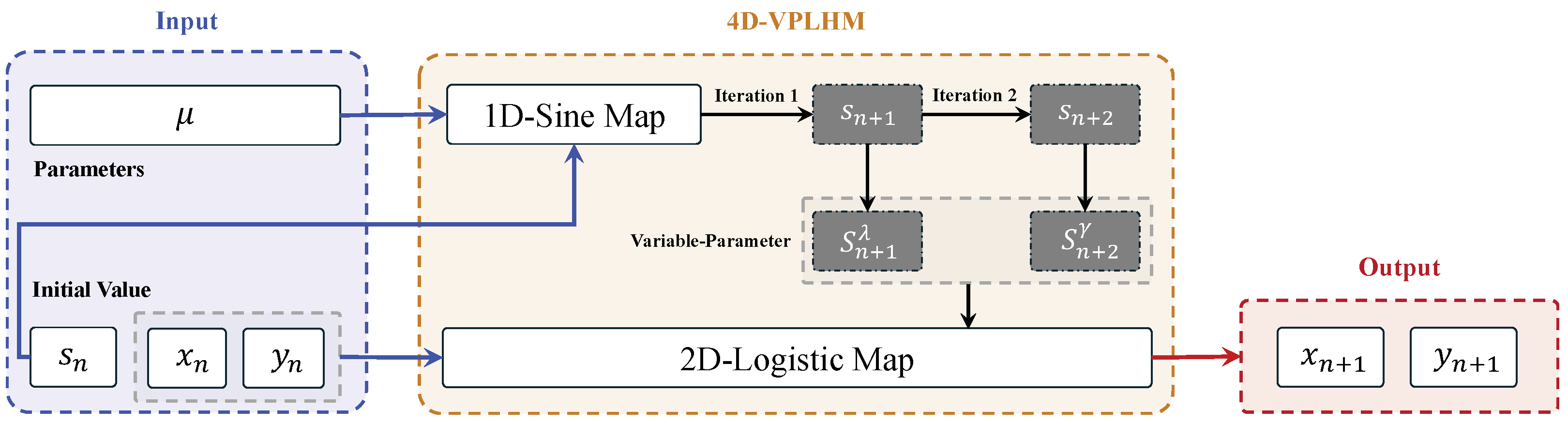
To overcome these limitations, we propose a novel four-dimensional chaotic system, termed the 4D variable-parameter logistic hybrid map (4D-VPLHM). This system dynamically incorporates the broad-range chaotic behavior of the 1D Sine map into the parameter modulation of the 4D coupled Logistic system. Specifically, the Sine map is used to generate a dynamic parameter sequence that drives the evolution of the Logistic map, thus enriching the system’s complexity. The structure of the proposed 4D-VPLHM is illustrated in Figure 1, and its mathematical definition is given as follows.
where the control parameters and are obtained by processing the Sine map outputs as follows:
where denotes the modulus operation. This transformation confines both parameters within the interval , a range known to lie within the chaotic regime of the Logistic map, thereby ensuring the system maintains robust chaotic dynamics throughout its evolution.
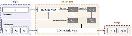
Figure 1.
The model structure of four-dimensional variable-parameter Logistic hyperchaotic map.
The 4D-VPLHM system is defined by one control parameter and four initial conditions , and it produces two output sequences . These design choices contribute to an enhanced key space, a higher-dimensional phase space, and increased sensitivity to initial conditions, which are critical for applications in secure communications and encryption.
2.2. Performance Evaluation
This section presents the simulation of the proposed 4D-VPLHM (four-dimensional variable-parameter Logistic hyperchaotic map) to assess its chaotic performance. To highlight the effectiveness of the proposed variable-parameter strategy, we compare it with several representative two-dimensional chaotic systems that share a similar design approach. Specifically, the following two-dimensional chaotic systems are considered for comparison.
The 2D-ICMIC-Logistic modulation map (2D-ILM) proposed by Cheng et al. [19] is as follows:
where is the control parameter.
The 2D absolute sine–cosine coupling (2D-ASCC) proposed by Zhang et al. [20] is as follows:
where is the control parameter.
The 2D cross-mode hyperchaotic map based on Logistic and Sine maps (2D-CLSS) proposed by Li et al. [4] is as follows:
where is the control parameter.
To ensure the rigor and fairness of the comparative experiments, all chaotic systems were initialized using the same settings. The initial values were randomly generated within the interval , and the total number of iterations was kept consistent across all systems. To allow for meaningful comparison, each chaotic system was evaluated under control parameters known to produce strong or representative chaotic behavior. Specifically, for the Sine map, we set , while for the 2D-ILM, 2D-ASCC, and 2D-CLSS systems, the parameters were set to , , and , respectively. For the 2D-Logistic system, we used and . For the proposed 4D-VPLHM, we chose based on its observed capacity to generate complex chaotic trajectories. These consistent and optimized parameter settings were adopted to highlight the dynamical features of each system and to objectively assess the performance of the proposed model.
2.2.1. Trajectory Diagram
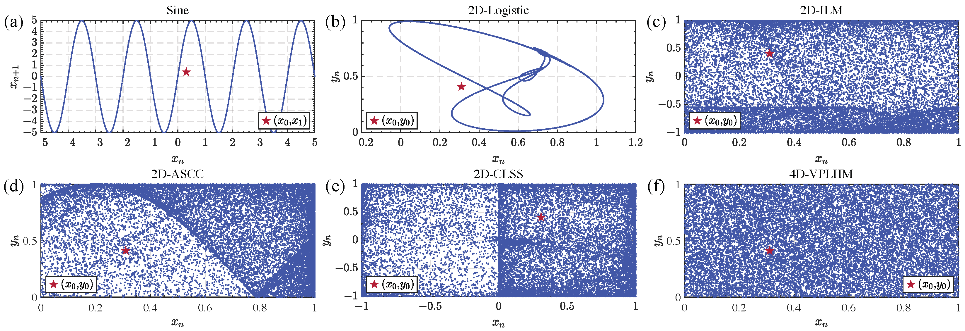
The trajectory plot of a chaotic system visually reflects the dynamic behavior of the system in generating random sequences. By analyzing the trajectory’s movement and distribution, one can assess the randomness and ergodicity of the generated sequences. To validate the superiority of the proposed 4D-VPLHM in generating random sequences, we analyzed its trajectory plot, as shown in Figure 2. For fairness and to emphasize the performance differences, all systems were initialized with the same initial conditions (e.g., ) and the same number of iterations (), and the first 1000 iterations were discarded.
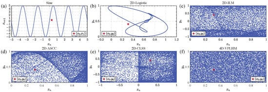
Figure 2.
Comparison results of the trajectory maps of chaotic systems: (a) Sine chaotic system, (b) 2D-Logistic chaotic system, (c) 2D-ILM chaotic system, (d) 2D-ASCC chaotic system, (e) 2D-CLSS chaotic system, (f) 4D-VPLHM chaotic system.
The classical Sine and 2D Logistic chaotic systems exhibit strong linearity in their random sequence trajectories, leading to limited phase space coverage and trajectories concentrated in specific regions. In contrast, while the 2D-ILM, 2D-ASCC, and 2D-CLSS chaotic systems cover the entire phase space, their trajectories still show significant clustering, indicating that the distribution is not uniform. The proposed 4D-VPLHM exhibits superior performance. Its trajectory is uniformly distributed and covers a wide area, with no obvious blank regions or clustering phenomena in phase space, indicating higher ergodicity and randomness in the generated sequences. The experimental results prove that the proposed variable-parameter strategy significantly improves the randomness and ergodicity of the chaotic system.
2.2.2. Bifurcation Diagram
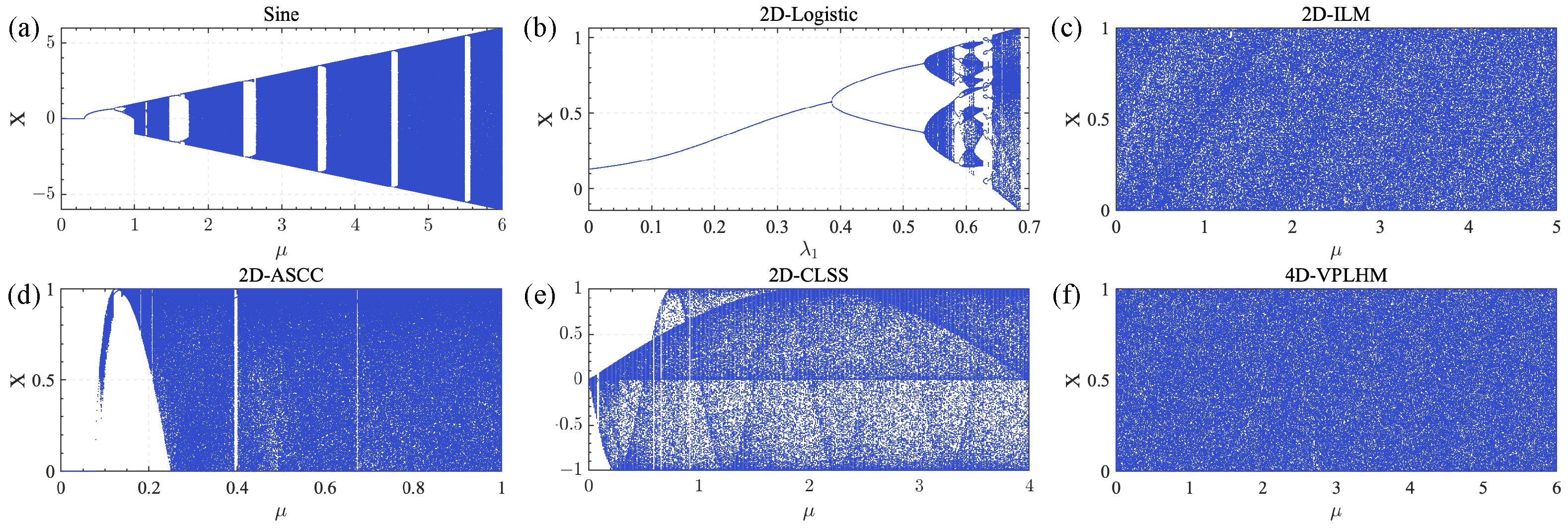
The bifurcation diagram is an important tool for analyzing the dynamic behavior of chaotic systems, visually revealing the system’s state evolution with parameter changes, especially the transition from periodic to chaotic states, and the instability and complexity of the system within the parameter range. Figure 3 presents the bifurcation diagram results for the proposed 4D-VPLHM and its comparison systems.
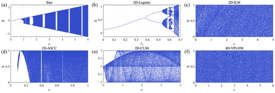
Figure 3.
Comparison results of bifurcation diagrams of chaotic system: (a) Sine chaotic system, (b) 2D-Logistic chaotic system, (c) 2D-ILM chaotic system, (d) 2D-ASCC chaotic system, (e) 2D-CLSS chaotic system, (f) 4D-VPLHM chaotic system.
For the classical Sine and 2D Logistic chaotic systems, the bifurcation diagrams indicate that as the control parameter changes, the system gradually transitions from a linear periodic state to a nonlinear chaotic state. However, their chaotic behavior is less persistent, with clear periodic windows within the chaotic region. In contrast, the 2D-ASCC and 2D-CLSS chaotic systems begin bifurcating at lower parameter values, with their bifurcation behavior covering a broader parameter range. However, as observed from the diagrams, both systems still exhibit periodic windows in their bifurcation paths and clustering within certain parameter ranges, indicating that their randomness and unpredictability remain constrained. The 2D-ILM and the proposed 4D-VPLHM show significant advantages. Both systems enter chaotic states within the initial parameter range and avoid periodic windows. Their bifurcation trajectories cover a broader parameter range, suggesting that the proposed variable-parameter strategy effectively enhances the system’s dynamic complexity and the stability of chaotic behavior.
2.2.3. Lyapunov Exponent
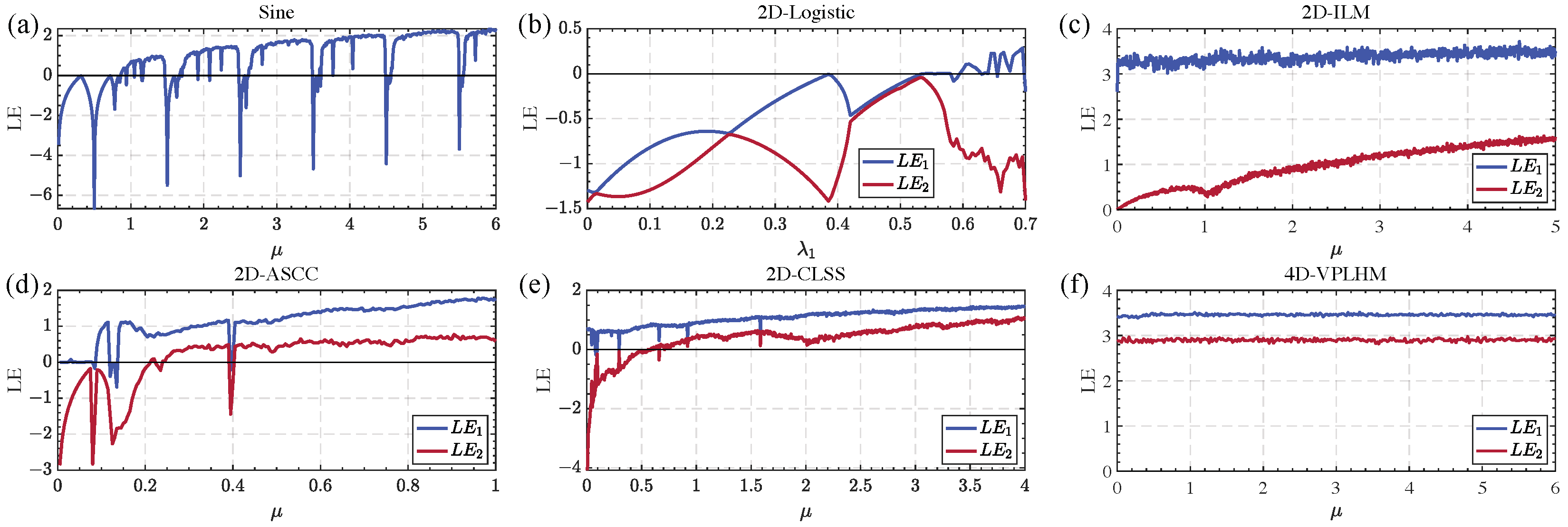
The Lyapunov exponent (LE) is a fundamental quantitative indicator used to evaluate the sensitivity of a dynamical system to initial conditions, thereby characterizing its chaotic behavior. In this paper, the maximum Lyapunov exponents are calculated using the algorithm proposed by Wolf et al. [21], which estimates the average exponential divergence of nearby trajectories reconstructed from the time series. For one-dimensional systems, a positive LE indicates chaos. For two-dimensional systems, if at least one exponent () is positive, the system is chaotic; if both and , the system exhibits hyperchaos, implying higher-dimensional dynamic complexity. Figure 4 illustrates the LE distributions of the proposed 4D-VPLHM and five other benchmark chaotic systems under varying control parameters.
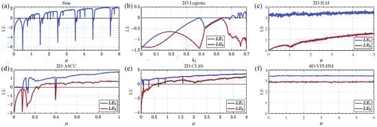
Figure 4.
Results of Lyapunov exponent comparison for chaotic systems: (a) Sine chaotic system, (b) 2D-Logistic chaotic system, (c) 2D-ILM chaotic system, (d) 2D-ASCC chaotic system, (e) 2D-CLSS chaotic system, (f) 4D-VPLHM chaotic system.
For the classical chaotic systems, Sine and 2D Logistic, as the control parameter changes, exhibits periodic fluctuations, becoming positive only within specific parameter ranges, indicating that the system can enter a chaotic state but with a narrow chaotic region. Additionally, for the 2D-Logistic system, remains less than zero, indicating that the system does not enter a hyperchaotic state. The improved 2D-ASCC and 2D-CLSS systems show that remains positive across a wider parameter range, and in certain intervals, , displaying hyperchaotic features. However, with parameter changes, the values of and fluctuate significantly, with frequent periodic windows, suggesting instability in chaotic behavior and poor robustness and controllability of dynamic performance. In contrast, the 2D-ILM shows significant advantages. Under parameter variation, its remains positive, indicating the system can continuously maintain a chaotic state. Moreover, rapidly reaches a positive value as the parameter increases and remains stable within a wide parameter range, demonstrating that the 2D-ILM can quickly enter a hyperchaotic state and maintain high dynamic complexity. However, there is still some fluctuation within certain parameter ranges, suggesting room for improvement in robustness. The proposed 4D-VPLHM demonstrates positive values for both Lyapunov exponents over all parameter ranges, indicating that the system remains stably in a hyperchaotic state across a wide parameter range. Unlike other systems, the Lyapunov exponent distribution of the 4D-VPLHM is much more stable, without significant fluctuations or obvious periodic windows, indicating that its dynamic behavior is more stable and robust.
2.2.4. Permutation Entropy
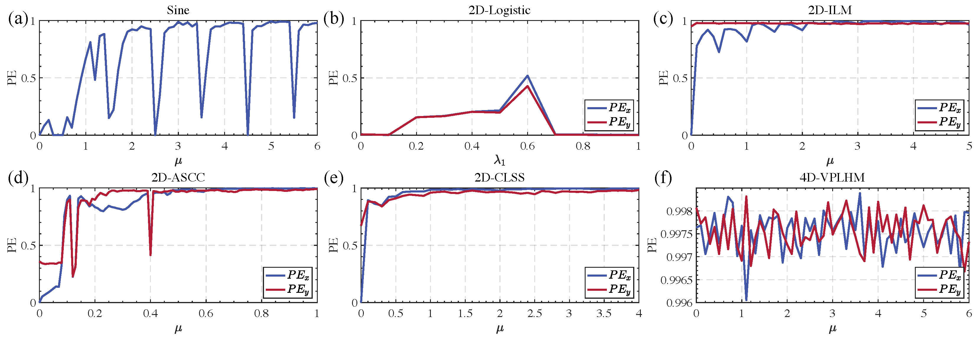
Permutation entropy (PE), introduced by Bandt and Pompe [22], is a robust and computationally efficient metric for evaluating the complexity of time series by quantifying the diversity of ordinal patterns. It reflects the degree of disorder in the system output: the higher the PE value, the stronger the randomness and unpredictability. In our study, PE is computed for the proposed 4D-VPLHM and five other classical or improved chaotic maps under varying control parameters, as shown in Figure 5.
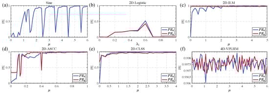
Figure 5.
Comparison results of permutation entropy: (a) Sine chaotic system, (b) 2D-Logistic chaotic system, (c) 2D-ILM chaotic system, (d) 2D-ASCC chaotic system, (e) 2D-ClSS chaotic system, (f) 4D-VPLHM chaotic system.
The results show that the PE of the classical Sine system exhibits significant periodic fluctuations as the parameter changes, with low entropy overall, only reaching higher values in certain parameter ranges, indicating poor randomness and instability. The 2D Logistic system shows nearly zero entropy over most parameter ranges, with a brief peak at , which quickly drops, indicating a lack of randomness and unpredictability in most cases. The 2D-ILM, 2D-ASCC, and 2D-CLSS systems gradually increase their entropy values as the control parameters increase, but their entropy values are not ideal at lower parameter values and are not stable. In particular, the 2D-ASCC shows a sharp decline in entropy around , which severely limits its use in encryption. In contrast, the proposed 4D-VPLHM exhibits stable, higher PE values across the full parameter range, indicating that the system consistently produces highly unpredictable sequences. The PE values show smooth transitions and high entropy across the entire parameter range, confirming that the proposed variable-parameter strategy can enhance the system’s randomness and unpredictability effectively, ensuring the system is suitable for secure encryption applications.
2.2.5. NIST Randomness Test
In cryptographic applications, the core role of chaotic systems in image encryption is to provide high-quality random sequences, which are essential for enhancing security. To evaluate the randomness of the proposed 4D-VPLHM chaotic system, we employed the NIST SP800-22 statistical test suite [23], which is designed for binary sequences. Since the output of the chaotic system consists of floating-point numbers, we first converted each value into its 64-bit binary representation using the IEEE 754 double-precision format [24]. Each generated sequence thus became a binary stream of length . We generated 150 such sequences with randomly selected parameters and , and we repeated the testing process 10 times for statistical reliability. We used the standard NIST evaluation metrics, including the pass rate and the average p-value, to assess randomness. The detailed test results are reported in Table 1.

Table 1.
NIST randomness test results for 4D-VPLHM.
For each test, with a significance level , if the p-value is greater than 0.01, the generated random sequence is considered random. For 150 test sequences, if 144 or more sequences pass the test (with a pass rate ), the test is considered successful. As shown in the table, considering the performance of both the P-value and pass rate, the chaotic sequences generated by the 4D-VPLHM passed all 15 tests. Furthermore, in over half of the tests conducted, the p-value exceeded 0.5, suggesting that the randomness performance of the proposed chaotic system is notably robust.
2.2.6. TestU01 Randomness Test
To further validate the randomness performance of the proposed 4D-VPLHM chaotic system, a more stringent TestU01 test suite [25] was used. In the experiment, all chaotic systems were initialized with the same initial conditions and configured to exhibit optimal performance. Sequences of length were generated and evaluated using the Alphabit, BlockAlphabit, and Rabbit tests, which contain 17, 102, and 39 sub-tests, respectively, designed to evaluate the quality of random sequences from various perspectives. The experimental results are shown in Table 2.
Table 2.
TestU01 randomness test results for six chaotic systems.
In all three tests, the proposed 4D-VPLHM demonstrated the best performance, surpassing both the classical Sine and 2D-Logistic systems. Additionally, it outperformed all the advanced methods, including 2D-ILM, 2D-CLSS, and 2D-ASCC, in every test item. These results further verify the excellent randomness of the proposed method.
3. A Fast Image Encryption Algorithm Based on the 4D-VPLHM and Circular Shift Strategy
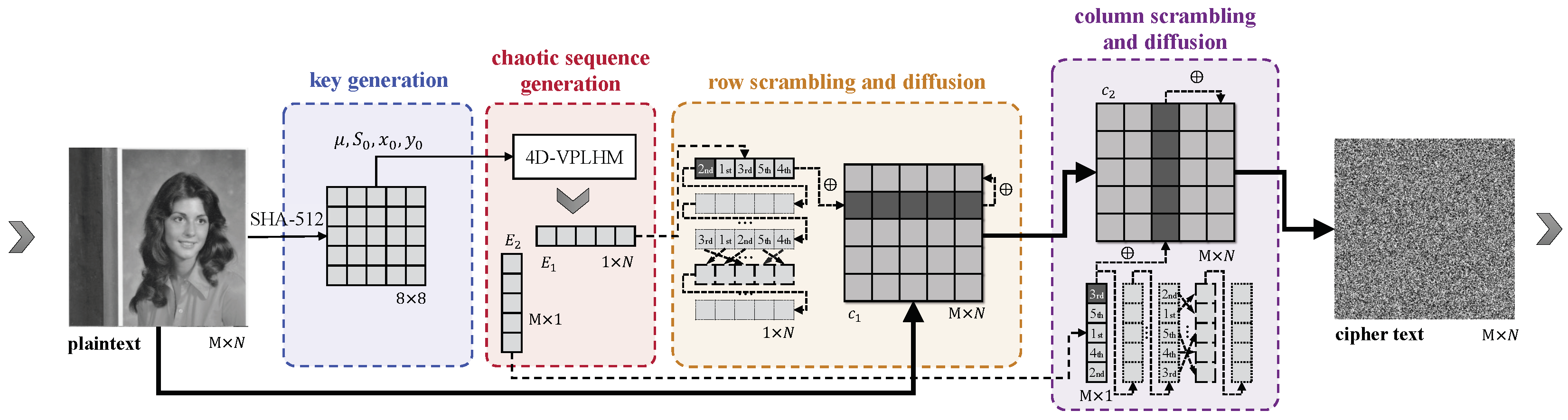
This section proposes a fast encryption algorithm at the row and column levels, based on the chaotic sequences generated by the 4D-VPLHM hyperchaotic system and the circular shift strategy. The core procedure of the algorithm is illustrated in Figure 6, which mainly consists of key generation, chaotic sequence generation, row scrambling and diffusion, and column scrambling and diffusion.
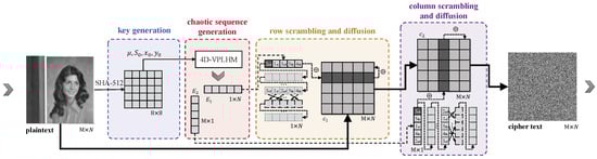
Figure 6.
Flowchart of the encryption scheme.
3.1. Key Generation
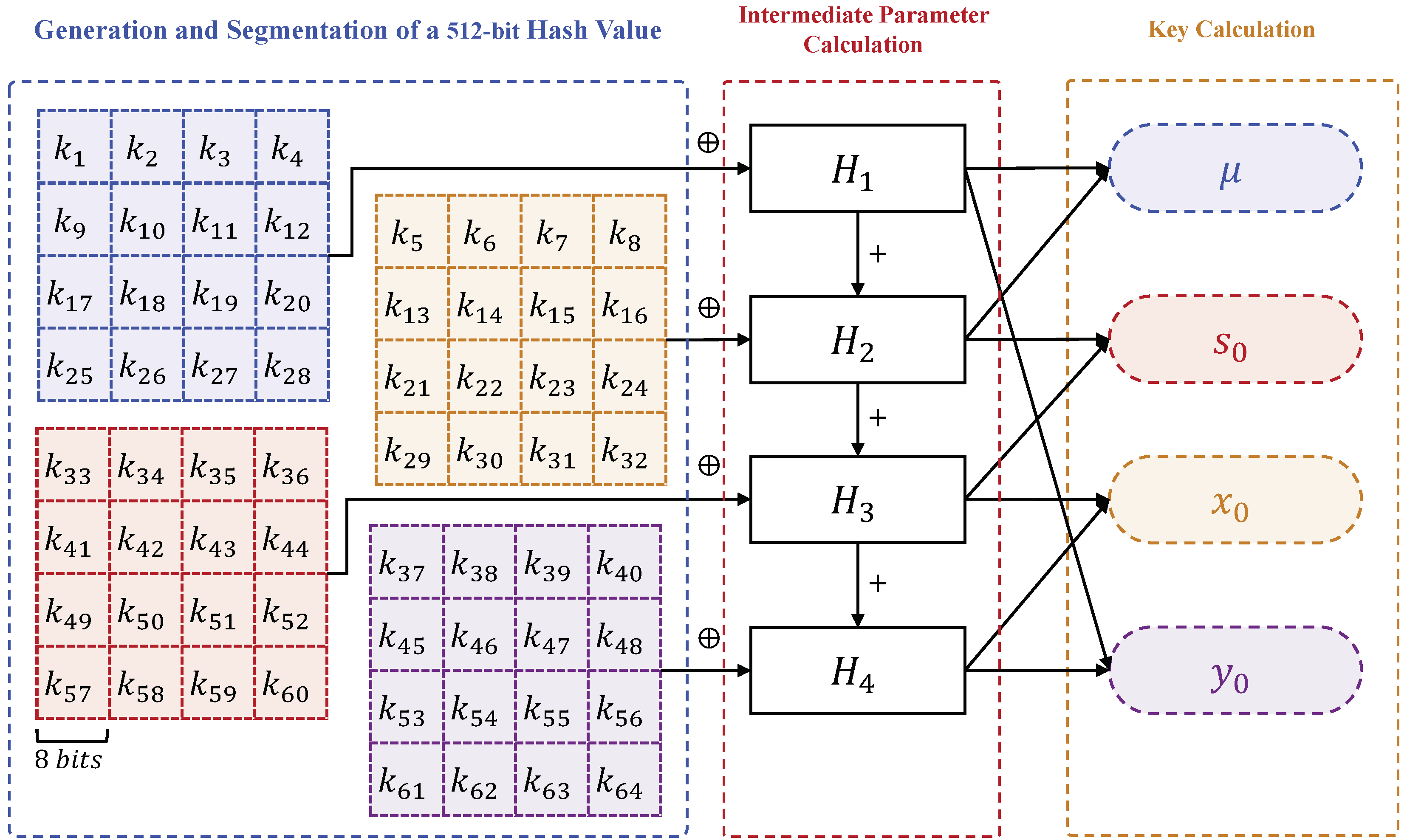
SHA-512, as a secure hashing algorithm, generates a 512-bit message digest for any given digital message. This digest is highly unique and irreversible. In our study, we utilize the SHA-512 algorithm to process the data of the image to be encrypted, generating a unique identifier closely related to the image content. Subsequently, based on this identifier, an algorithm is designed to compute the control parameters and initial values required for the chaotic encryption process. These parameters and values serve as the encryption key, ensuring that the encryption process is directly tied to the plaintext image content. The detailed process is shown in Figure 7.
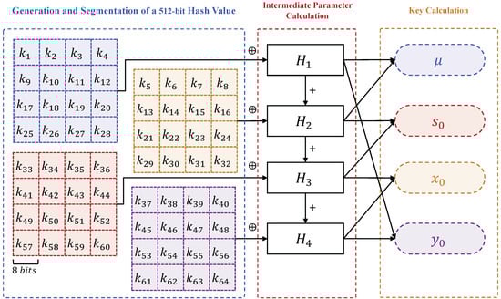
Figure 7.
Flowchart of key generation algorithm.
The detailed steps for key generation are as follows:
- Generation and segmentation of a 512-bit hash value: To initialize the encryption process, the plaintext image is first processed using the SHA-512 cryptographic hash function, yielding a 512-bit binary string. This binary output is then partitioned into 64 segments of 8 bits each, with each segment converted into a corresponding decimal value in the range of 0 to 255. These values are denoted as . Following the segmentation scheme illustrated in the corresponding flowchart, the 64 decimal values are subsequently divided into four groups, each comprising 16 elements.
- Intermediate parameter calculation: For each group, an XOR operation is performed on all values, and the result is divided by 255 to generate 4 intermediate parameters, denoted as . The specific calculation method is as follows:
- Key calculation: Through the combination of four intermediate variables, the control parameters and initial values required by 4D-VPLHM are obtained. The calculation method is as follows:where the value of is in the range , and the values of , , and are all ion the range . These values serve as the key control parameters and initial values for the chaotic encryption process, ensuring a direct correlation between the encryption process and the plaintext image content.
3.2. Encryption Algorithm
The control parameters and initial values are input into the 4D-VPLHM chaotic system for iterative computation, generating two chaotic sequences with the same length as the image’s row and column dimensions. These sequences serve as the random sources for row and column scrambling–diffusion encryption, respectively. Subsequently, the circular shift algorithm is applied to continuously generate new chaotic sequences from the 1D chaotic sequences for XOR-based encryption of each row and column in the image. Each encryption operation involves the result from the previous encryption step. The entire encryption algorithm requires only one round of scrambling and diffusion to produce the encrypted image while meeting the security and effectiveness requirements for digital image encryption algorithms. The detailed computational steps are as follows:
- Input: Plaintext image P, of size , encryption key .
- Output: Ciphertext image C, of size .
- Step 1: Chaotic sequence generation:The key is input into the 4D-VPLHM chaotic system for iterations, where T is a constant, with chosen in this study. To eliminate transient phenomena in the chaotic system, the first T output sequences are discarded. From the x and y outputs of 4D-VPLHM, two chaotic sequences and of length are obtained.
- Step 2: Row and column diffusion rules generation: From the output , the first M elements are selected to obtain the chaotic sequence of size , which has the same length as the number of elements in each row of the plaintext image P, serving as the initial row diffusion rule. Similarly, from the output , the first N elements are selected to obtain the chaotic sequence of size , serving as the initial column diffusion rule.
- Step 3: Row and column scrambling rules generation: The chaotic sequence is sorted in ascending order to obtain its corresponding index sequence of size , which serves as the row scrambling rule. Similarly, the column scrambling rule is obtained from the chaotic sequence of size .
- Step 4: Row scrambling and diffusion: Using the row scrambling rule, one row at a time is selected from the plaintext image P as the target for encryption. This process constitutes the scrambling operation. The diffusion rule is then applied, converting the target row into an integer sequence between 0 and 255, which is XORed with the corresponding row of the plaintext. If it is not the first row, the result is further XORed with the previously encrypted row, forming the diffusion operation. After each diffusion, the decimal elements of the diffusion rule are cyclically shifted left by one position, yielding a new diffusion sequence for the next row. After 15 shifts, a row-wise scrambling operation is applied to the diffusion rule based on the magnitude relationships of the previous encryption results, preventing identical diffusion rules from occurring. This process is referred to as the circular shift algorithm. A computational example of this process is shown in Figure 8. The detailed steps of row scrambling and diffusion are as follows:
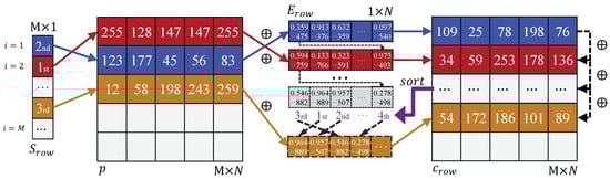 Figure 8. Example of row scrambling and diffusion encryption procedures.
 - Step 4.1: Initialization: Initialize the ciphertext storage matrix of size .Step 4.2: Row scrambling: Traverse the row scrambling rule in order, and for each index i (where ), select the i-th row of the plaintext image as the target for diffusion encryption.
- Step 4.3: Row diffusion: XOR the selected row with the row diffusion rule to obtain the encrypted row, which is placed in the ciphertext at the i-th position. For , the result is further XORed with the previous row in the ciphertext. The diffusion rule is as follows:where represents the floor function and represents the modulus function.
- Step 4.4: Circular shift: After completing the encryption for each row, the row diffusion rule is cyclically shifted left by one position for use as the scrambling rule for the next row. After completing 15 shifts (corresponding to the effective precision of 16 digits for double-precision floating-point numbers), a row-wise scrambling operation is performed on the diffusion rule based on the relative magnitude of elements in the previously encrypted row to avoid duplicate diffusion rules during the shifting process. The circular shift operation is as follows:where denotes the cyclic shift of the decimal positions of array elements, refers to the sorted index array, and represents the diffusion rule array rearranged according to the index sequence x. Once the scrambling traversal is complete, the row scrambling and diffusion process is finished.
- Step 5: Column scrambling and diffusion: The column scrambling and diffusion processes follow the same strategy as the row processes. The encryption object is the result of the row scrambling and diffusion, . The column scrambling rule is applied to perform the column scrambling operation, and the column diffusion rule is used for the diffusion operation. After each column is encrypted, the column diffusion rule undergoes the same circular shift operation. The final encrypted image C is obtained after completing the scrambling and diffusion of all columns.
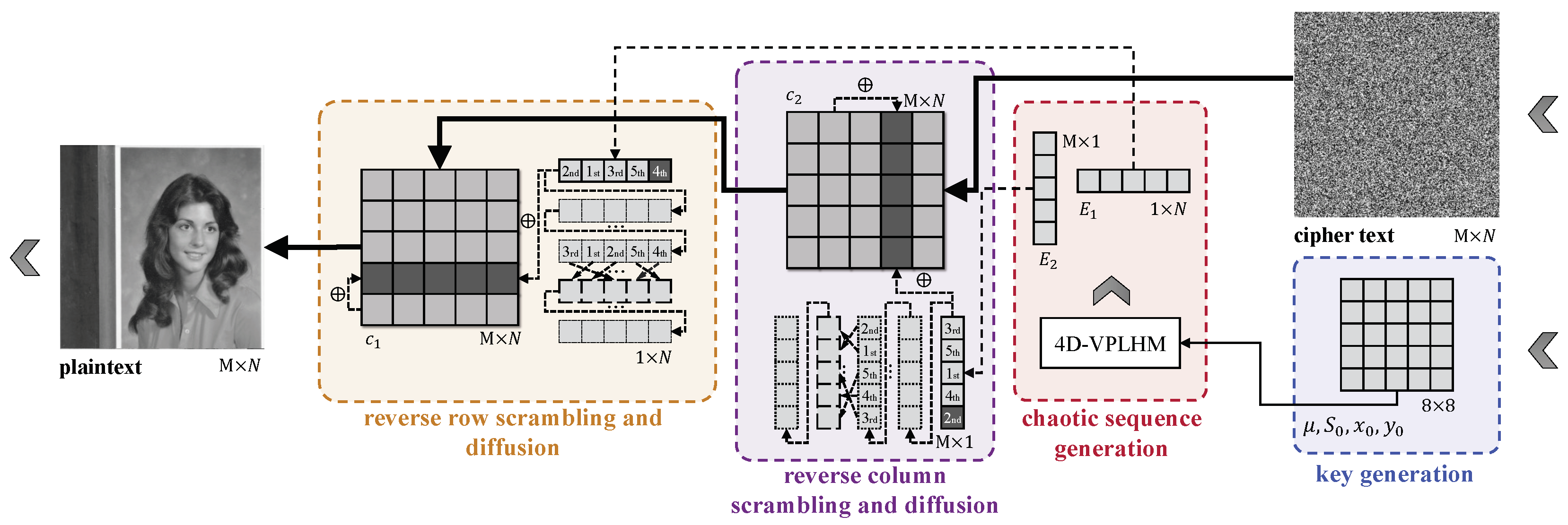
3.3. Decryption Algorithm
In this paper, the image encryption is implemented using a reversible XOR operation. Consequently, the decryption of the encrypted image can be achieved through the inverse process. The flowchart of the decryption algorithm is shown in Figure 9.
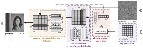
Figure 9.
Decryption scheme flowchart.
- Input: Ciphertext image C of size and key .
- Output: Plaintext image P of size .
- Step 1: Generation of the chaotic sequences. The chaotic sequences and are generated following Step 1 of the encryption algorithm.
- Step 2: Generation of the row and column diffusion rules. The row and column diffusion rules are derived in accordance with Step 2 of the encryption algorithm.
- Step 3: Generation of the row and column scrambling rules. The row and column scrambling rules are obtained according to Step 3 of the encryption algorithm.
- Step 4: Inverse column scrambling and diffusion. Each column of the ciphertext is traversed sequentially as the target for decryption. The column diffusion rule is applied to the corresponding column, and XOR decryption is performed. If the current row is not the first row, the result is further XORed with the corresponding row of the previous column; this is the inverse diffusion process. After the inverse diffusion is completed, the decrypted result is placed back into its original position according to the column scrambling rule, which completes the inverse scrambling process. After each row decryption, the column diffusion rule is cyclically shifted in the same manner as the encryption process. Detailed steps for row scrambling and diffusion are as follows:
- Step 4.1: Initialization. Initialize the plaintext storage matrices and , both of size .
- Step 4.2: Inverse Column diffusion. Traverse each column of the ciphertext C, with the current position denoted as i, where . The first column is selected as the target for inverse diffusion decryption. The column diffusion rule is XORed with the column to be decrypted. For , the XOR result is further XORed with the previous column of ciphertext. The inverse diffusion rule is as follows:
- Step 4.3: Inverse column scrambling. After the column decryption is complete, the decrypted column is placed in the correct position in the plaintext using the column scrambling rule . The inverse column scrambling rule is given by
- Step 4.4: Cyclic shifting. The column cyclic shifting operation is performed according to Step 4.4 of the encryption process.
- Step 5: Inverse row scrambling and diffusion. Following the same procedure as the inverse column scrambling and diffusion, the decryption target is the result of inverse column scrambling and diffusion . The row scrambling rule is used to perform the inverse row scrambling, while the row diffusion rule is applied to reverse the diffusion operation. After each column is diffused, the column diffusion rule is cyclically shifted according to the same rules as the encryption process. Once the row scrambling is complete, the final decrypted result P is obtained.
4. Improved Binary Level NPCR and UACI
4.1. NPCR and UACI
The Number of Pixels Change Rate (NPCR) is a metric used to quantify the difference between two images by comparing the pixel values at corresponding positions. If the pixel values differ, the number of differing pixels is recorded. After the entire image is traversed, the proportion of differing pixels relative to the total number of pixels is computed to provide a quantitative description of the image difference. Let and represent the two compared images, both of size with 256 grayscale levels. The NPCR is calculated as shown in Equation (14):
where the function represents the sign function. It is defined as 0 when the pixel values at the corresponding positions are the same and 1 when the pixel values differ. Thus,
The theoretical value of NPCR for two random images is .
The Uniform Average Changing Intensity (UACI) is used to measure the average intensity of pixel changes between two images. It calculates the pixel-wise differences between the two images at corresponding positions, normalizing them relative to the maximum possible difference (255), and then computes the average of these normalized differences across all pixels. The mathematical definition of UACI is shown in Equation (16):
The theoretical value of NPCR for two random images is .
Although NPCR and UACI are important metrics for measuring the similarity between two images, they have certain limitations in specific cases. For NPCR, when two images differ at all corresponding pixel positions, it reaches its theoretical maximum. However, if the differences between the pixel values are minimal, NPCR might indicate a large change between the images, even though they visually appear almost identical. For example, we created a new image by adding 1 to every pixel value of the Female image. The NPCR value of the new image is , but visually it remains highly similar to the original image. This suggests that relying solely on NPCR to evaluate the differences between images can be misleading.
UACI partially addresses this limitation of NPCR by not only considering whether a pixel has changed but also quantifying the magnitude of the change. However, due to the theoretical value of UACI being , a pixel difference of approximately 85 is sufficient to achieve this value for grayscale images with 256 levels. In such cases, although UACI reaches its ideal value, the overall visual effect of the image might still be quite similar to the original. As shown in Figure 10c,d, Figure 10c was created by adding 85 to each pixel of the original image, resulting in NPCR reaching and UACI approaching its theoretical value. Similarly, Figure 10d was constructed by flipping half of the pixel values and modifying the other half by just one grayscale level, also resulting in NPCR and UACI values near the theoretical values. However, visually, the image retains substantial information from the original. This demonstrates that even when NPCR and UACI values are high, if the encryption system is weak and the encrypted image retains visible information from the original, these metrics may still overestimate the encryption effectiveness.
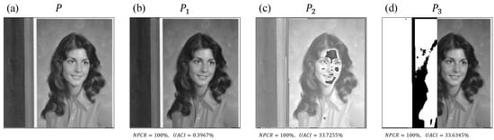
Figure 10.
Images constructed based on the original Female image. (a) The original Female image. (b) Constructed image , obtained by adding 1 to each pixel value of the original image. (c) Resultant image , obtained by applying a pixel difference of 85 to every pixel value of the original image. (d) Resultant image , obtained by inverting half of the pixels of the original image and applying a pixel difference of 1 to the remaining half.
4.2. BL-NPCR and BL-UACI
Motivated by the sensitivity analysis of traditional NPCR and UACI metrics to high pixel values, this section proposes an enhanced evaluation strategy by modifying the number of pixel bits used in the computation. For an 8-bit grayscale image, each pixel value ranges from 0 to 255 and can be represented by 8 binary bits. The contribution of the i-th bit to the actual pixel intensity can be quantified as
The contribution of each bit position is summarized in the Table 3.
Table 3.
The percentage of information content carried by different bits.
As observed, the higher 4 bits (i.e., bits 5 through 8) collectively account for 93.1% of the total pixel information. This dominant proportion indicates that variations in these bits correspond to perceptually significant and substantial changes in image content, while differences in the lower bits primarily reflect trivial or noise-level fluctuations. Consequently, to reduce excessive sensitivity to negligible changes, we propose to compute the evaluation metrics based only on the top 4 bits of the pixel values.
Accordingly, we introduce two modified metrics for assessing the resistance of encryption schemes against differential attacks: Binary-Level Number of Pixels Change Rate (BL-NPCR) and Binary-Level Unified Average Changing Intensity (BL-UACI). These metrics operate at the binary level of pixel values and aim to achieve a better balance between robustness and representative accuracy in evaluating encryption performance.
The calculation process for BL-NPCR and BL-UACI consists of the following two steps:
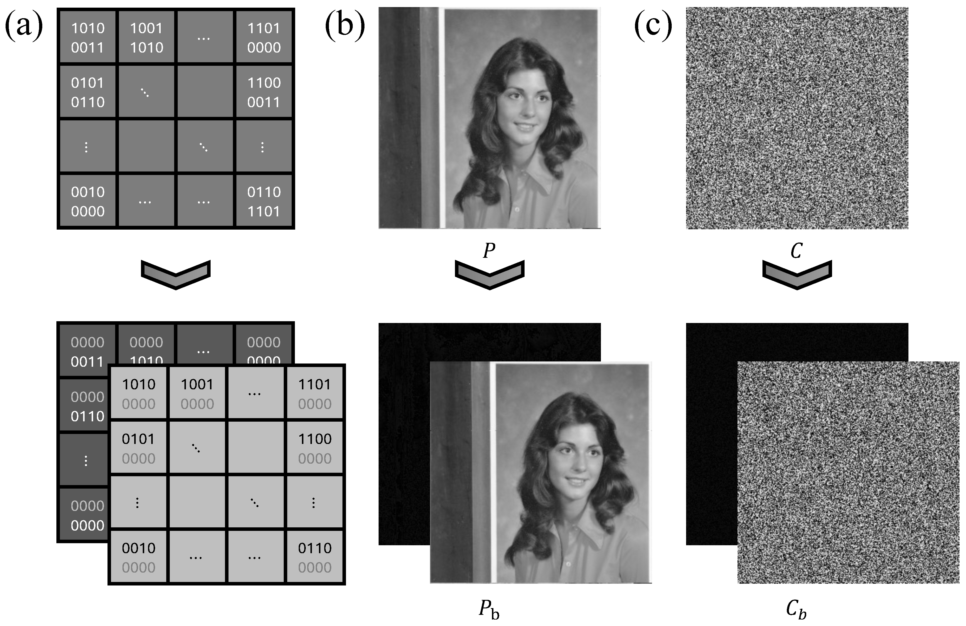
(1) Binary partitioning: Before calculating the metrics, the two images to be compared are subject to bit-plane decomposition. Specifically, for each pixel value in the image, only the higher 4 bits are retained, and the lower 4 bits are set to zero, resulting in a new image. This process is denoted as and is defined by the following equation:
where ∧ denotes the bitwise AND operation, and 240 (binary: 11110000) is used to preserve the higher 4 bits and zero out the lower 4 bits.
Since the higher 4 bits of the pixel value provide a relatively accurate representation of the image’s overall information, the image obtained after binary partitioning visually differs little from the original, though the overall brightness is reduced. An example of the original image after binary partitioning is shown in Figure 11.
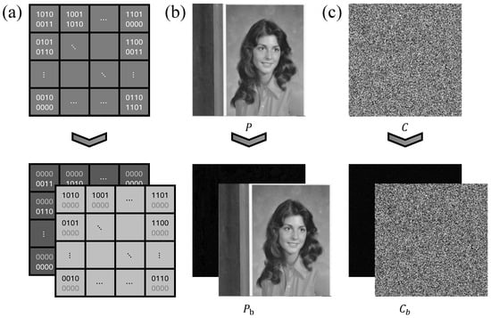
Figure 11.
Binary partition example. (a) Example of pixel value bit-plane decomposition. (b) Bit-plane decomposition of Female pixel values. (c) Bit-plane decomposition of pixel values in random pixel maps.
(2) BL-NPCR and BL-UACI calculation: Once the binary partitioning is complete, the NPCR and UACI calculation methods are applied to the partitioned images, specifically calculating the pixel change rate and intensity. Let and represent the two images, and the formulas for calculating BL-NPCR and BL-UACI are as follows:
where BL-Sign is an improved sign function applied to the binary partitioned pixel values, defined as follows:
(3) Theoretical values: The range of BL-NPCR is 0–100%, and its expected value can be expressed as
For two random images, the probability of change at a given pixel position is as follows:
Thus, the theoretical expected value of BL-NPCR is calculated as follows:
BL-UACI’s range is also 0–100%, with larger values indicating greater difference between the images. The expected value of BL-UACI is calculated as
After binary partitioning, pixel values are reduced from 256 levels to 16 levels, with pixel differences ranging from to 240. The probability of each optional value is
The expected value of BL-UACI is calculated as
Performance Analysis
The metrics were computed for the three images constructed earlier, and the results are presented in Table 4.
Table 4.
BL-NPCR and BL-UACI calculation results for Female image.
The results indicate that although NPCR and UACI yield high values in certain cases, BL-NPCR and BL-UACI more accurately reflect the true differences between the images. In situations where the visual effect is similar but traditional metrics show high values, BL-NPCR and BL-UACI exhibit a significant deviation from their theoretical values, further confirming their advantage in quantifying the differences between images.
5. Simulation and Analysis
In order to verify the security and feasibility of the algorithm proposed in this chapter, five representative test images were selected, including natural images (Female and Boat), texture images (Gray), text images (Text), and medical images (X-ray). Additionally, 211 images from The USC-SIPI Image Database [26] were used as an extra test set to ensure the comprehensiveness and diversity of the analysis. The hardware environment for the experiment was a CPU Intel Core i7 2.6 GHz processor, 16GB memory, and Windows 10 operating system. The software environment was MATLAB 2016b.
5.1. Simulation Results
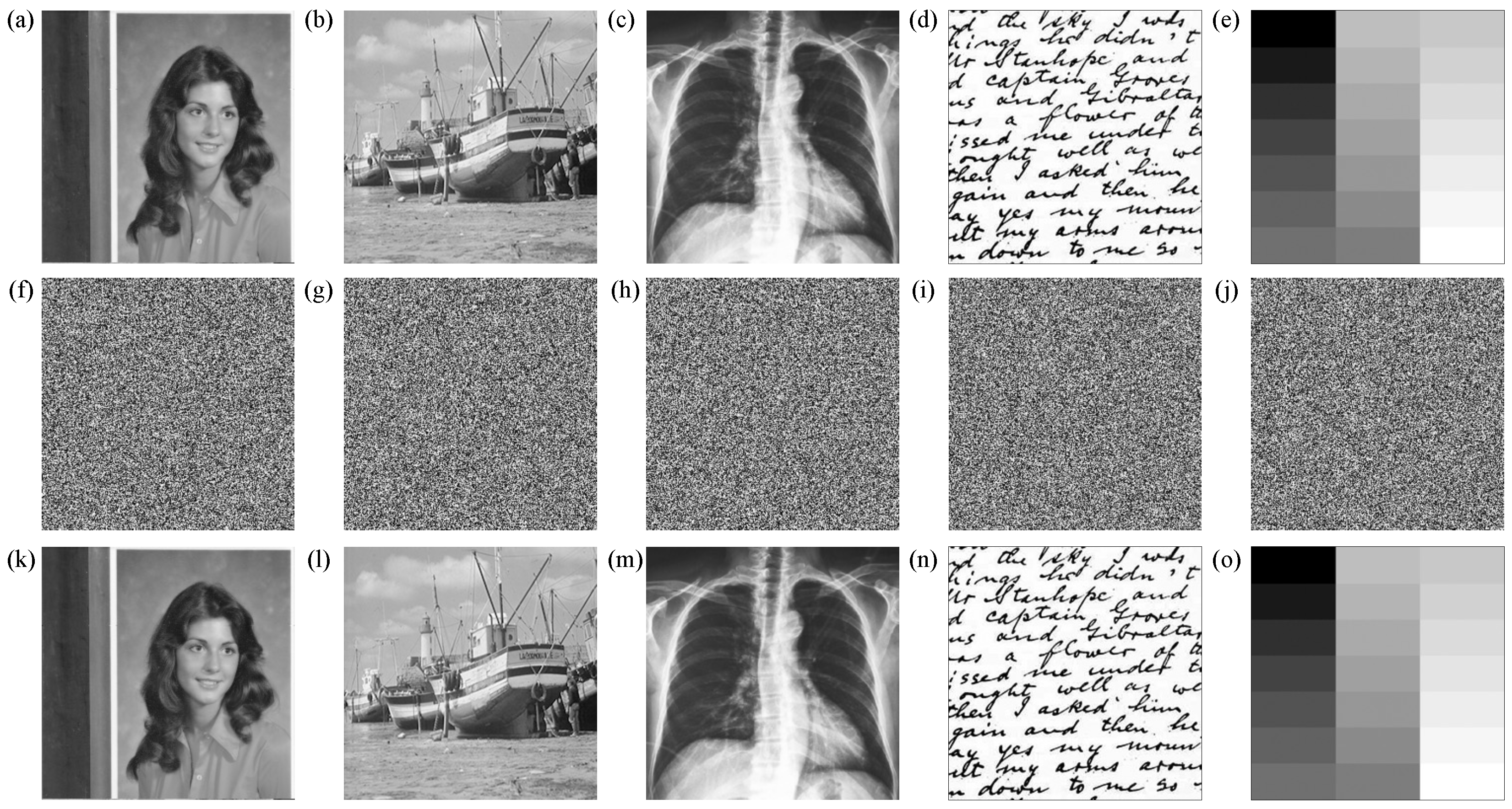
Figure 12 illustrates the encryption and decryption effects of the proposed encryption system on various test images. The first row shows the original test images, the second row shows the corresponding encrypted images, and the third row shows the images restored by the decryption algorithm.
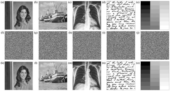
Figure 12.
Encryption and decryption simulation results. (a–e) Original images of Female, Boat, Gray, Text, and X-ray, respectively. (f–j) Encrypted images of Female, Boat, Gray, Text, and X-ray, respectively. (k–o) Decrypted images of Female, Boat, Gray, Text, and X-ray, respectively.
From the result, it can be observed that the proposed encryption algorithm successfully transforms the original images into encrypted images resembling random noise, effectively hiding all identifiable information. The decryption algorithm is capable of accurately recovering the encrypted images, maintaining consistency with the original images. Even for the Gray image, which has a regionally repetitive pixel distribution, the encryption algorithm is able to break its inherent regularity, demonstrating its resistance to chosen-plaintext attacks.
5.2. Key Space and Key Sensitivity Analysis
The algorithm proposed in this paper uses the SHA-512 algorithm to derive a 512-bit sequence from the plaintext image, which is then linearly combined with an initial value to generate the initial values and control parameters used by the encryption system. Therefore, the key space is . Given the current computational performance of computers, it is impossible to crack this key using brute-force attacks [27].
To verify the key sensitivity of the proposed algorithm, Female was used as the test image. The hash value at the i-th position after modification is denoted as . The first and last positions of each block in Figure 7 (, , , , , , , and ) were selected as representatives. Subsequently, the modified key was employed to decrypt the image that had been encrypted using the correct key. Some decryption results are presented in Figure 13.
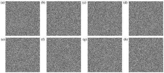
Figure 13.
Female figure key sensitivity test results. (a–h), respectively, shows the , , , , , , , position decryption result after key change.
From Figure 13, it can be seen that even a slight change in the key (altering only one bit) leads to significant changes in the decrypted image. Each minor adjustment in the key completely prevents the recovery of the original image, indicating that the proposed encryption algorithm is highly sensitive to key changes. This sensitivity ensures the security of the algorithm and effectively prevents key prediction attacks, thus enhancing the encryption system’s resistance to attacks.
5.3. Robustness of the Cyclic Shift Algorithm
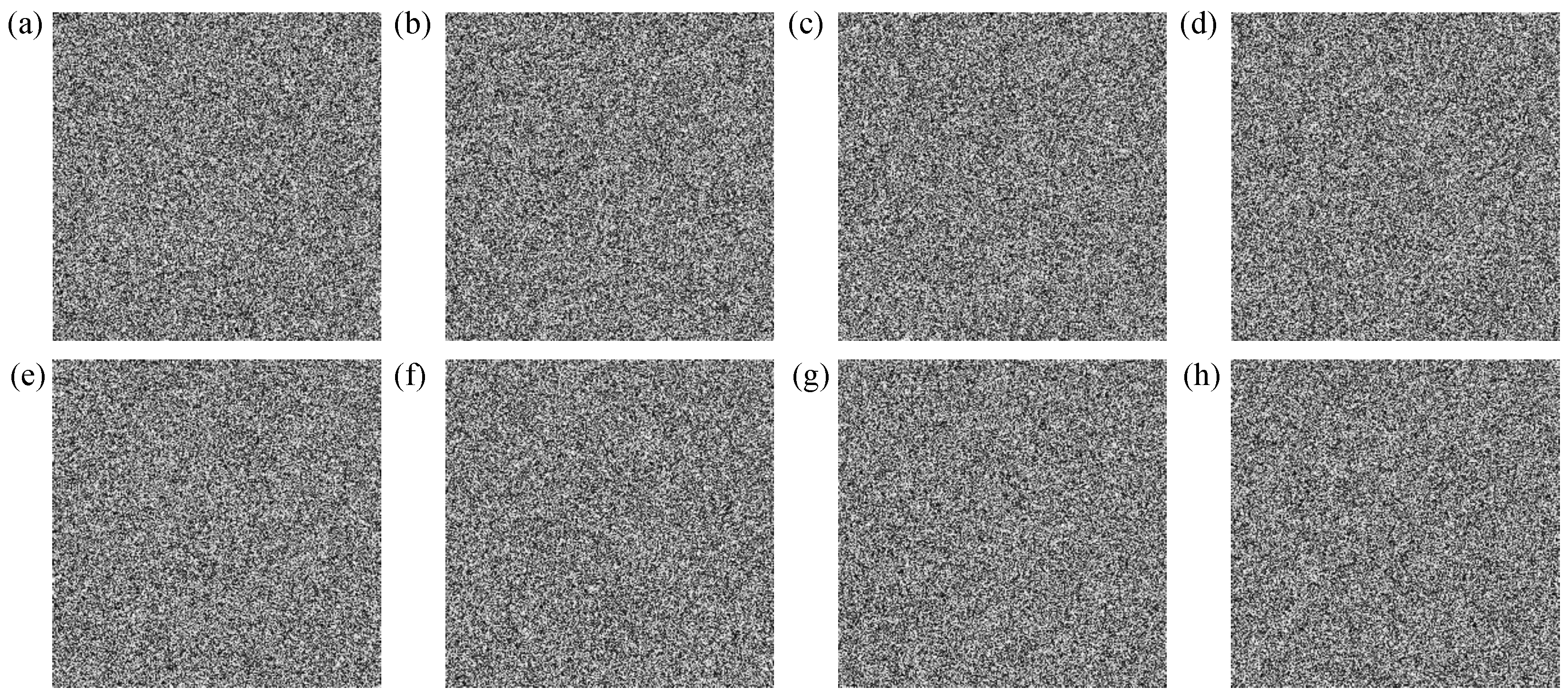
The encryption algorithm proposed in this paper relies on a cyclic shift algorithm, which generates random sequences from a finite chaotic sequence for use in encryption. To verify whether the chaotic sequences generated by the cyclic shift algorithm meet the needs of the encryption algorithm and to compare their differences with sequences directly generated from the 4D variable-parameter logistic map (4D-VPLHM), this section provides a thorough verification of the randomness of the chaotic sequences generated by the cyclic shift algorithm. Specifically, the chaotic sequence is set to a length of . Sequence x is the output of the 4D-VPLHM chaotic system after iterations; sequence y is based on the iterations of x from the 4D-VPLHM chaotic system, which is then processed by the cyclic shift algorithm for iterations and concatenated. Additionally, to evaluate the effectiveness of the in-row scrambling operation in the cyclic shift algorithm, we recorded the results without the in-row scrambling operation, denoted as sequence z.
The NIST randomness test results for the three types of chaotic sequences are shown in Table 5. The NIST test results show that the y sequence, after cyclic shifting, passed all the test items, indicating that the cyclic shift strategy can effectively retain the randomness of the original sequence while expanding the data length, meeting the strict randomness requirements of secure encryption algorithms. However, upon observing the results for the z sequence, it was found that the randomness level drastically dropped after removing the in-row scrambling operation, passing only three tests. This highlights the critical role of the in-row scrambling operation in maintaining the chaotic performance.
Table 5.
NIST randomness test results of the cyclic shift algorithm.
Further, we conducted the TestU01 test and efficiency tests for the generation of chaotic sequences, with results shown in Table 6. The TestU01 results further confirm the aforementioned conclusion. The chaotic sequence y shows only a slight decrease in performance compared to the 4D-VPLHM in three of the tests but still maintains high randomness. In terms of time efficiency, generating a chaotic sequence of length with the cyclic shift algorithm requires only seconds, whereas generating the same sequence directly via 4D-VPLHM takes seconds, resulting in a significant speedup. Thus, the cyclic shift algorithm effectively accelerates the chaotic sequence generation process while ensuring randomness, achieving an efficiency approximately twice that of the approach without the cyclic shift strategy.
Table 6.
TestU01 randomness test results and time consumption comparison of the cyclic shift algorithm.
5.4. Histogram Analysis
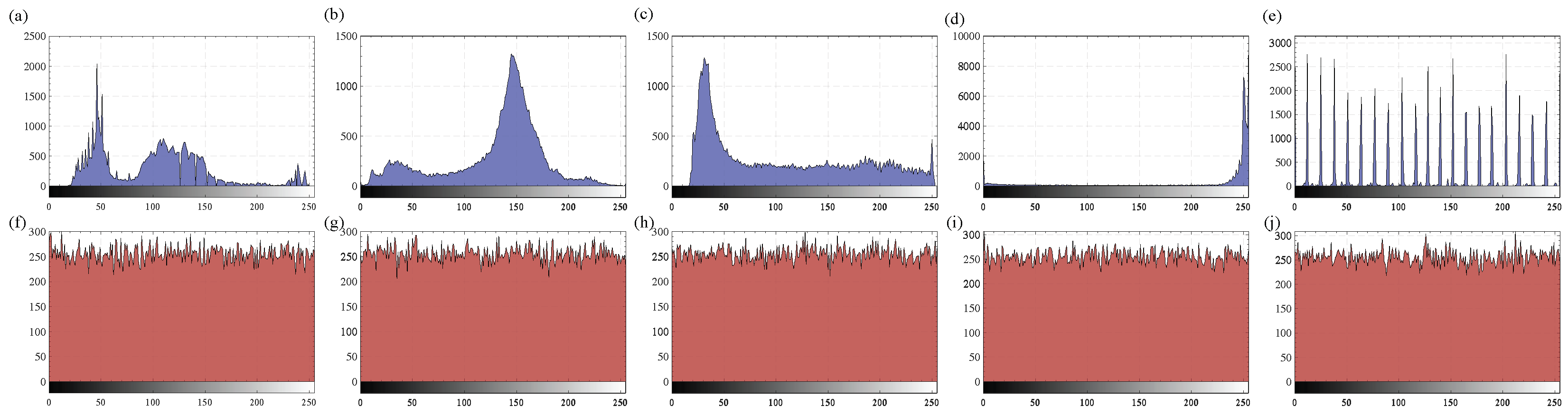
Digital images carry visual information through the distribution of their pixel values. These pixel values are typically concentrated within certain ranges, manifesting as statistically significant patterns in the color channels of the image. The histogram is an intuitive tool for reflecting the distribution of pixels, and by observing the shape of the histogram, we can gather statistical characteristics about the image information. Figure 14 shows the histogram changes of the test image before and after encryption.
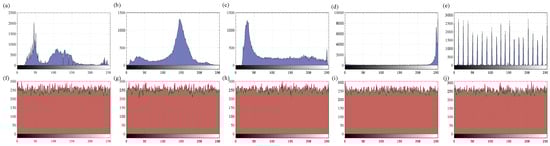
Figure 14.
Histogram analysis results for test images before and after encryption. (a–e) represent the histograms of the original images for Female, Boat, Gray, Text, and X-ray, respectively. (f–j) represent the histograms of the encrypted images for Female, Boat, Gray, Text, and X-ray, respectively.
From the figure, it can be observed that before encryption, the histogram of the test image exhibits clear concentration, with pixel values concentrated in specific ranges, reflecting the statistical regularity of the image. However, after encryption, the histogram of the image shows a more uniform distribution of pixel values, making it difficult to discern any obvious patterns. This indicates that the proposed encryption algorithm has successfully disrupted the statistical properties of the original image, making the pixel value distribution more uniform, thus effectively resisting attacks based on image statistical properties.
5.5. Information Entropy Analysis
Information entropy is a crucial metric for measuring the randomness and information content of image pixels. It quantitatively describes the degree of disorder in the pixel values and the uniformity of their distribution. In image encryption, a higher entropy value indicates a more uniform pixel distribution, making it harder to predict. For a 256-level grayscale image, the theoretical maximum entropy value is 8. The formula for calculating information entropy is
where is the probability of a pixel having value i.
Table 7 presents the entropy values before and after encryption for different test images. It can be observed that the entropy of the encrypted images is significantly higher than that of the original images and approaches the theoretical maximum value of 8. This indicates that the pixel distribution of the encrypted images is nearly uniform, greatly enhancing their information content, and making it impossible to extract any useful information through simple statistical analysis.
Table 7.
Information entropy test results.
Furthermore, we compared the encryption entropy values of the proposed algorithm with several existing encryption methods applied to the Lena image. Table 8 shows that the entropy value of the proposed algorithm’s encrypted image is 7.9993, significantly higher than that of other methods, indicating that the proposed algorithm performs best in increasing entropy.
Table 8.
Information entropy comparison results for the Lena image.
5.6. Correlation Analysis of Adjacent Pixels
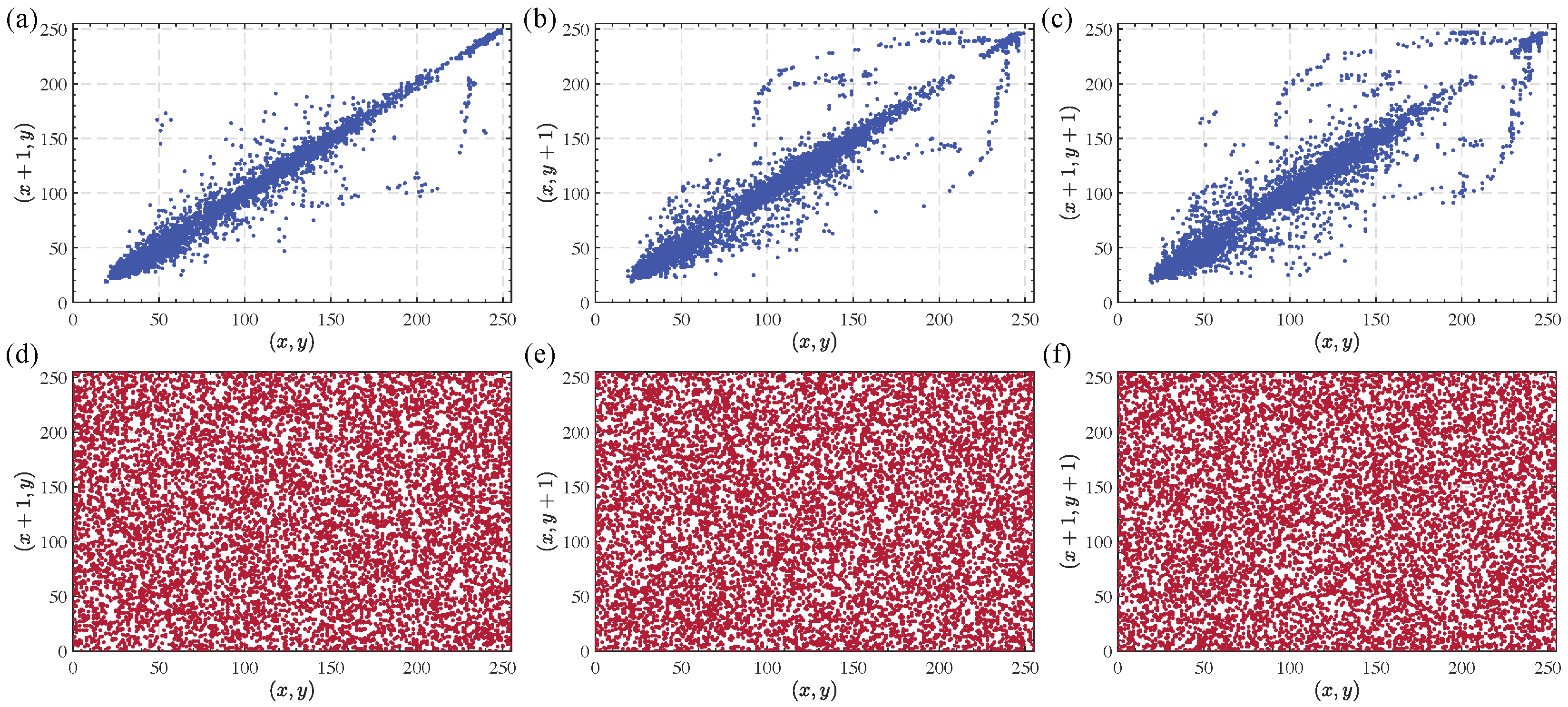
In natural images, there is typically a strong correlation between adjacent pixels, which allows for the use of statistical properties in image compression, transmission, and analysis. The effectiveness of an encryption algorithm is often measured by its ability to destroy this inherent correlation, thereby enhancing the security of the image. To evaluate the ability of the proposed encryption algorithm to break down the correlation between adjacent pixels, this section analyzes the Female image before and after encryption. We randomly selected 5000 pixels from both the encrypted and original images and visualized their distributions in the horizontal, vertical, and diagonal directions. Figure 15 shows these distributions.

Figure 15.
Adjacent pixel distribution of the Female image before and after encryption. (a–c) depict the distributions of adjacent pixels in the horizontal, vertical, and diagonal directions for the original Female image. (d–f) illustrate the corresponding distributions for the encrypted Female image.
From the figure, it is clear that the unencrypted image exhibits noticeable clustering in all three directions, showing high correlation, meaning that adjacent pixels are highly linearly related. In contrast, the encrypted image shows a more uniform and random distribution of pixel values, with no apparent pattern in any of the three directions, further proving that the proposed algorithm effectively disrupts the pixel correlation and increases the randomness and security of the image. To quantitatively analyze the correlation between pixels, we used the Pearson correlation coefficient, calculated as follows:
where represents the mean of the pixel values and represents the variance. The calculated correlation coefficient quantifies the linear relationship between two pixel values.
Table 9 presents the correlation coefficients of test images in the horizontal, vertical, and diagonal directions before and after encryption. As observed, the original images exhibit high correlation in all three directions. However, after encryption, these correlation coefficients drop to values close to zero, indicating that the pixel distribution has become nearly random and the original correlation has been effectively eliminated.
Table 9.
Adjacent pixel correlation results before and after encryption of the test image.
Furthermore, we compare the encryption performance of the proposed algorithm with several existing encryption algorithms on the Lena image. Table 10 presents the correlation coefficients of adjacent pixels in different directions after encryption. As shown in the table, the proposed algorithm achieves the lowest correlation coefficients in all three directions, indicating its superior effectiveness in eliminating pixel correlations.
Table 10.
Comparison of adjacent pixel correlation after encryption of Lena image using different algorithms.
5.7. Differential Attack Analysis
Differential attacks are a type of chosen plaintext attack in which the attacker analyzes the impact of small changes in the plaintext pixels on the resulting ciphertext, aiming to deduce the key or the structure of the encryption algorithm. To ensure the security of the encryption system, an ideal algorithm should exhibit high sensitivity, meaning that even a slight change in a single pixel of the plaintext should result in a ciphertext that appears completely random, preventing the attacker from extracting useful information through differential analysis. To evaluate the proposed algorithm’s resistance to differential attacks, NPCR, UACI, BL-NPCR, and BL-UACI are used as evaluation metrics. In the ideal case, the theoretical values of these metrics are , , , and , respectively, indicating that the differences between the two images should follow a random distribution.
In the experiment, we randomly selected one pixel from the test image, increased its grayscale value by 1, and then applied the proposed encryption algorithm to both the original and modified images. The NPCR, UACI, BL-NPCR, and BL-UACI values of the ciphertexts were calculated, and the experiment was repeated 100 times to obtain statistical averages. Table 11 summarizes the average values after 150 rounds of calculation.
Table 11.
Differential analysis results of test images.
From Table 11, it is evident that the proposed encryption algorithm performs excellently on the four key performance indicators. Specifically, for the five test images, the average deviations of the indicators from the theoretical expected values are all within , strongly validating the algorithm’s high sensitivity to small changes in the plaintext and its significant diffusion effect. Notably, the average performance on the SIMP dataset further reduced this deviation to below , demonstrating a significant improvement in the stability of the method and further reinforcing its reliability in practical applications.
To further evaluate the advantages of the proposed method, we compared it with existing similar algorithms. Table 12 lists the NPCR, UACI, BL-NPCR, and BL-UACI results for different algorithms applied to the Lena image, along with the deviations from the theoretical values in parentheses. The data show that the proposed algorithm consistently outperforms the other methods, indicating that it offers superior security against differential attacks.
Table 12.
Comparison of differential analysis results of different algorithms on the Lena image.
5.8. Encryption Efficiency Analysis
Improving the encryption efficiency of an algorithm while maintaining its security is a key goal in image encryption research. To evaluate the encryption efficiency of the proposed algorithm, we analyze its performance using encryption time, encryption throughput (ET), and the number of cycles per byte (NCPB). The calculations for ET and the number of cycles are as follows:
The encryption time in our experiments includes the total time required for key generation, chaotic sequence generation, row scrambling and diffusion, and column scrambling and diffusion. To ensure the reliability of the results, we applied the proposed algorithm to the Female image for 100 independent encryption operations and calculated the average encryption time. The experimental results are summarized in Table 13.
Table 13.
Encryption algorithm efficiency analysis results.
From Table 13, it can be observed that the proposed algorithm achieves the shortest encryption time in experiments with images of three different sizes. Additionally, its encryption throughput is higher than existing schemes, and the number of cycles per byte is lower. This demonstrates that the proposed algorithm, while ensuring security, also achieves high computational efficiency, making it suitable for real-time encryption applications. Further analysis of the encryption time consumption across different image sizes reveals that when the image size is increased by a factor of four, the encryption time for other methods increases nearly fourfold, showing a clear linear growth trend. In contrast, the proposed algorithm, thanks to the unique advantages of the cyclic shift algorithm, does not exhibit a proportional increase in time consumption as the image size grows. This phenomenon illustrates the proposed algorithm’s superiority in handling larger images and avoiding additional computational overhead caused by chaotic sequence generation, thus enhancing overall encryption efficiency.
To validate this mechanism further, we encrypted Female images of different resolutions and calculated the average encryption time. In addition, we designed two baseline algorithms (Baseline1 and Baseline2) to compare the computational efficiency of traditional encryption schemes:
- Baseline1: This uses the same row–column permutation and diffusion algorithms, but the chaotic sequence is generated over iterations (equal to the total number of pixels in the image).
- Baseline2: This uses a simple pixel value encryption algorithm, and the chaotic sequence is generated over iterations.
In the experiment, we selected image sizes ranging from to , with a step size of 16, and executed 100 encryption operations for each size, calculating the average encryption time and variance. The experimental results are shown in Figure 16.
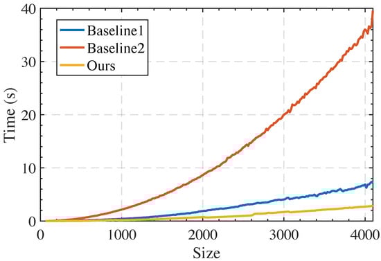
Figure 16.
Comparison of image encryption time for different sizes.
From the results, we can observe that as the image size increases, the encryption time for Baseline2 grows the fastest, followed by Baseline1. In contrast, the encryption time for the proposed method increases the slowest. This indicates that for large image encryption tasks, traditional methods experience performance degradation due to the high computational cost of chaotic sequence generation, whereas the proposed cyclic shift mechanism effectively reduces the time consumed by chaotic sequence generation, enabling better adaptation to large-scale image encryption needs. Moreover, throughout the entire size range, the proposed algorithm’s computational efficiency remains stable, demonstrating excellent scalability and computational advantages.
6. Conclusions
With the rapid advancement of network technology, the transmission of digital images over the internet has become increasingly frequent, raising significant security concerns, particularly for confidential and personal image data. Chaos-based encryption schemes, owing to their inherent randomness and sensitivity to initial conditions, have been widely recognized as effective solutions. To address the limitations of traditional chaotic systems this paper proposes a novel four-dimensional variable-parameter hyperchaotic map (4D-VPLHM) by integrating the one-dimensional Sine chaotic map and the two-dimensional Logistic map. The proposed chaotic system exhibits a broader hyperchaotic range and complex, unpredictable dynamics, enabling the generation of high-quality random sequences. Based on this system, we develop a fast image encryption algorithm that leverages a cyclic shift strategy to continuously generate high-randomness chaotic sequences from a relatively small-scale seed sequence. This mechanism significantly enhances encryption efficiency and security, making the proposed algorithm well suited for handling large-scale image encryption tasks in real-time scenarios.
Furthermore, to overcome the limitations of conventional differential attack resistance metrics, we introduce an improved evaluation metric based on binary-level pixel partitioning which assess variation intensity and rate at the binary representation level. Experimental results confirm that these refined metrics provide a more precise and objective assessment of encryption resistance against differential attacks, effectively addressing the shortcomings of conventional evaluation methods.
Comprehensive experimental evaluations demonstrate the computational efficiency, security robustness, and practical applicability of the proposed encryption scheme. Compared with existing methods, our approach achieves higher encryption speed, enhanced differential attack resistance, and reduced computational overhead, making it highly suitable for large-scale and real-time image encryption applications.
Although the proposed scheme demonstrates strong performance in grayscale image encryption, several avenues remain open for future exploration. First, while the variable-parameter scheme has proven effective in enhancing the chaotic behavior of low-dimensional systems, future research could investigate more lightweight or structure-adaptive variants to achieve higher efficiency in resource-constrained environments. Second, the binary-level differential metrics proposed in this work provide a more stable evaluation framework; however, their current design relies on a fixed high-bit selection. Future studies may explore more adaptive or weighted schemes to further improve metric robustness across diverse application scenarios. Third, as the present encryption design targets grayscale images, extending the approach to color images—potentially by modeling interchannel correlations—could enhance its applicability and security.
Author Contributions
Conceptualization, G.Z. and Y.Z. (Yanhao Zhao); methodology, G.Z.; Software, G.Z.; validation, G.Z., Y.Z. (Yanhao Zhao) and Y.Z. (Yanpei Zheng); formal analysis, G.Z.; investigation, G.Z.; resources, G.Z.; data curation, G.Z.; writing—original draft preparation, G.Z.; writing—review and editing, J.H.; visualization, G.Z.; supervision, Y.S. and J.H.; project administration, J.H.; funding acquisition, Y.S. All authors have read and agreed to the published version of the manuscript.
Funding
This work was supported in part by the Central Guidance for Local Science and Technology Development Funds Project under grant number 25ZYJA039, and in part by the Key Talent Project of Gansu Province.
Data Availability Statement
Dataset available on request from the authors.
Acknowledgments
The authors gratefully acknowledge the anonymous reviewers for their helpful comments and suggestions.
Conflicts of Interest
Author Yanpei Zheng was employed by the company Gansu Civil Aviation Airport Group Co., Ltd. The remaining authors declare that the research was conducted in the absence of any commercial or financial relationships that could be construed as a potential conflict of interest.
References
- Li, Y.; Wang, C.; Chen, H. A Hyper-Chaos-Based Image Encryption Algorithm Using Pixel-Level Permutation and Bit-Level Permutation. Opt. Lasers Eng. 2017, 90, 238–246. [Google Scholar] [CrossRef]
- ur Rehman, A.; Liao, X.; Ashraf, R.; Ullah, S.; Wang, H. A Color Image Encryption Technique Using Exclusive-OR with DNA Complementary Rules Based on Chaos Theory and SHA-2. Optik 2018, 159, 348–367. [Google Scholar] [CrossRef]
- Shannon, C.E. Communication Theory of Secrecy Systems. Bell Syst. Tech. J. 1949, 28, 656–715. [Google Scholar] [CrossRef]
- Teng, L.; Wang, X.; Xian, Y. Image Encryption Algorithm Based on a 2D-CLSS Hyperchaotic Map Using Simultaneous Permutation and Diffusion. Inf. Sci. 2022, 605, 71–85. [Google Scholar] [CrossRef]
- Fridrich, J. Symmetric Ciphers Based on Two-Dimensional Chaotic Maps. Int. J. Bifurc. Chaos 1998, 8, 1259–1284. [Google Scholar] [CrossRef]
- Lin, C.Y.; Wu, J.L. Cryptanalysis and Improvement of a Chaotic Map-Based Image Encryption System Using Both Plaintext Related Permutation and Diffusion. Entropy 2020, 22, 589. [Google Scholar] [CrossRef] [PubMed]
- Hu, Y.; Yu, S.; Zhang, Z. On the Security Analysis of a Hopfield Chaotic Neural Network-Based Image Encryption Algorithm. Complexity 2020, 2020, 2051653. [Google Scholar] [CrossRef]
- Li, Z.; Peng, C.; Li, L.; Zhu, X. A Novel Plaintext-Related Image Encryption Scheme Using Hyper-Chaotic System. Nonlinear Dyn. 2018, 94, 1319–1333. [Google Scholar] [CrossRef]
- Chen, Y.; Xie, S.; Zhang, J. A Hybrid Domain Image Encryption Algorithm Based on Improved Henon Map. Entropy 2022, 24, 287. [Google Scholar] [CrossRef]
- Zhang, Y.; Tang, Y. A Plaintext-Related Image Encryption Algorithm Based on Chaos. Multimed. Tools Appl. 2018, 77, 6647–6669. [Google Scholar] [CrossRef]
- Su, Y.; Wang, X.; Gao, H. Chaotic Image Encryption Algorithm Based on Bit-Level Feedback Adjustment. Inf. Sci. 2024, 679, 121088. [Google Scholar] [CrossRef]
- Gao, X. Image Encryption Algorithm Based on 2D Hyperchaotic Map. Opt. Laser Technol. 2021, 142, 107252. [Google Scholar] [CrossRef]
- Naskar, P.K.; Bhattacharyya, S.; Mahatab, K.C.; Dhal, K.G.; Chaudhuri, A. An Efficient Block-Level Image Encryption Scheme Based on Multi-Chaotic Maps with DNA Encoding. Nonlinear Dyn. 2021, 105, 3673–3698. [Google Scholar] [CrossRef]
- Hu, G.; Li, B. Coupling Chaotic System Based on Unit Transform and Its Applications in Image Encryption. Signal Process. 2021, 178, 107790. [Google Scholar] [CrossRef]
- Zhang, X.; Liu, G.; Niu, Y.; Zou, C. Color Image Encryption Scheme Based on a Single Attractor Hyperchaotic System and Go Rules. Nonlinear Dyn. 2025, 113, 13885–13911. [Google Scholar] [CrossRef]
- Hu, G.; Li, B. A Uniform Chaotic System with Extended Parameter Range for Image Encryption. Nonlinear Dyn. 2021, 103, 2819–2840. [Google Scholar] [CrossRef]
- Li, S.; Yin, B.; Ding, W.; Zhang, T.; Ma, Y. A Nonlinearly Modulated Logistic Map with Delay for Image Encryption. Electronics 2018, 7, 326. [Google Scholar] [CrossRef]
- Gui, X.; Huang, J.; Li, L.; Li, S.; Cao, J. A Novel Hyperchaotic Image Encryption Algorithm with Simultaneous Shuffling and Diffusion. Multimed. Tools Appl. 2022, 81, 21975–21994. [Google Scholar] [CrossRef]
- Huang, X.; Tang, J.; Zhang, Z. Efficient and Secure Image Encryption Algorithm Using 2D LIM Map and Latin Square Matrix. Nonlinear Dyn. 2024, 112, 22463–22483. [Google Scholar] [CrossRef]
- Fei, X.; Zhang, J.; Qin, W. Design a New Image Encryption Algorithm Based on a 2D-ASCC Map. Phys. Scr. 2022, 97, 125206. [Google Scholar] [CrossRef]
- Wolf, A.; Swift, J.B.; Swinney, H.L.; Vastano, J.A. Determining Lyapunov Exponents from a Time Series. Phys. D Nonlinear Phenom. 1985, 16, 285–317. [Google Scholar] [CrossRef]
- Bandt, C.; Pompe, B. Permutation Entropy: A Natural Complexity Measure for Time Series. Phys. Rev. Lett. 2002, 88, 174102. [Google Scholar] [CrossRef] [PubMed]
- Bassham, L.; Rukhin, A.; Soto, J.; Nechvatal, J.; Smid, M.; Leigh, S.; Levenson, M.; Vangel, M.; Heckert, N.; Banks, D. A Statistical Test Suite for Random and Pseudorandom Number Generators for Cryptographic Applications. 2010. Available online: https://tsapps.nist.gov/publication/get_pdf.cfm?pub_id=906762 (accessed on 26 February 2025).
- Sahari, M.L.; Boukemara, I. A Pseudo-Random Numbers Generator Based on a Novel 3D Chaotic Map with an Application to Color Image Encryption. Nonlinear Dyn. 2018, 94, 723–744. [Google Scholar] [CrossRef]
- L’Ecuyer, P.; Simard, R. TestU01: A C Library for Empirical Testing of Random Number Generators. ACM Trans. Math. Softw. 2007, 33, 22:1–22:40. [Google Scholar] [CrossRef]
- SIPI Image Database. 2024. Available online: https://sipi.usc.edu/database/ (accessed on 26 February 2025).
- Alvarez, G.; Li, S. Some Basic Cryptographic Requirements for Chaos-Based Cryptosystems. Int. J. Bifurc. Chaos 2006, 16, 2129–2151. [Google Scholar] [CrossRef]
- Shariatzadeh, M.; Rostami, M.J.; Eftekhari, M. Proposing a Novel Dynamic AES for Image Encryption Using a Chaotic Map Key Management Approach. Optik 2021, 246, 167779. [Google Scholar] [CrossRef]
- Çavuşoğlu, Ü.; Kaçar, S.; Pehlivan, I.; Zengin, A. Secure Image Encryption Algorithm Design Using a Novel Chaos Based S-box. Chaos Solitons Fractals 2017, 95, 92–101. [Google Scholar] [CrossRef]
- Zhou, S.; Wang, X.; Zhang, Y.; Ge, B.; Wang, M.; Gao, S. A Novel Image Encryption Cryptosystem Based on True Random Numbers and Chaotic Systems. Multimed. Syst. 2022, 28, 95–112. [Google Scholar] [CrossRef]
- Xu, Y.; Liu, J.; You, Z.; Zhang, T. A Novel Color Image Encryption Algorithm Based on Hybrid Two-Dimensional Hyperchaos and Genetic Recombination. Mathematics 2024, 12, 3457. [Google Scholar] [CrossRef]
- Hosny, K.M.; Kamal, S.T.; Darwish, M.M. Novel Encryption for Color Images Using Fractional-Order Hyperchaotic System. J. Ambient. Intell. Humaniz. Comput. 2022, 13, 973–988. [Google Scholar] [CrossRef]
- Shi, L.; Li, X.; Jin, B.; Li, Y. A Chaos-Based Encryption Algorithm to Protect the Security of Digital Artwork Images. Mathematics 2024, 12, 3162. [Google Scholar] [CrossRef]
- Wang, W.t.; Sun, J.y.; Zhang, H.; Zhang, J. Quantum Cryptosystem and Circuit Design for Color Image Based on Novel 3D Julia-Fractal Chaos System. Quantum Inf. Process. 2023, 22, 64. [Google Scholar] [CrossRef]
- Yu, F.; Tan, B.; He, T.; He, S.; Huang, Y.; Cai, S.; Lin, H. A Wide-Range Adjustable Conservative Memristive Hyperchaotic System with Transient Quasi-Periodic Characteristics and Encryption Application. Mathematics 2025, 13, 726. [Google Scholar] [CrossRef]
- Sarosh, P.; Parah, S.A.; Bhat, G.M. An Efficient Image Encryption Scheme for Healthcare Applications. Multimed. Tools Appl. 2022, 81, 7253–7270. [Google Scholar] [CrossRef] [PubMed]
- Xu, J.; Zhao, B.; Wu, Z. Research on Color Image Encryption Algorithm Based on Bit-Plane and Chen Chaotic System. Entropy 2022, 24, 186. [Google Scholar] [CrossRef]
- Sivakumar, T.; Li, P. A Secure Image Encryption Method Using Scan Pattern and Random Key Stream Derived from Laser Chaos. Opt. Laser Technol. 2019, 111, 196–204. [Google Scholar] [CrossRef]
- Liu, H.; Xu, Y.; Ma, C. Chaos-Based Image Hybrid Encryption Algorithm Using Key Stretching and Hash Feedback. Optik 2020, 216, 164925. [Google Scholar] [CrossRef]
- Farah, M.A.B.; Guesmi, R.; Kachouri, A.; Samet, M. A Novel Chaos Based Optical Image Encryption Using Fractional Fourier Transform and DNA Sequence Operation. Opt. Laser Technol. 2020, 121, 105777. [Google Scholar] [CrossRef]
- Vidhya, R.; Brindha, M. A Chaos Based Image Encryption Algorithm Using Rubik’s Cube and Prime Factorization Process (CIERPF). J. King Saud Univ. Comput. Inf. Sci. 2022, 34, 2000–2016. [Google Scholar] [CrossRef]
- Kaur, G.; Agarwal, R.; Patidar, V. Chaos Based Multiple Order Optical Transform for 2D Image Encryption. Eng. Sci. Technol. Int. J. 2020, 23, 998–1014. [Google Scholar] [CrossRef]
- Wang, M.; Teng, L.; Zhou, W.; Yan, X.; Xia, Z.; Zhou, S. A New 2D Cross Hyperchaotic Sine-Modulation-Logistic Map and Its Application in Bit-Level Image Encryption. Expert Syst. Appl. 2025, 261, 125328. [Google Scholar] [CrossRef]
- Zou, C.; Shang, Y.; Yang, Y.; Zhou, C.; Liu, Y. A Novel Image Encryption Algorithm with Anti-Tampering Attack Capability. Chaos Solitons Fractals 2024, 189, 115638. [Google Scholar] [CrossRef]
- Lu, J.; Zhang, J.; An, D.; Hao, D.; Ren, X.; Zhao, R. A Low-Time-Consumption Image Encryption Combining 2D Parametric Pascal Matrix Chaotic System and Elementary Operation. J. King Saud Univ. Comput. Inf. Sci. 2024, 36, 102169. [Google Scholar] [CrossRef]
- Alawida, M. A Novel Chaos-Based Permutation for Image Encryption. J. King Saud Univ. Comput. Inf. Sci. 2023, 35, 101595. [Google Scholar] [CrossRef]
- Jiang, X.; Jiang, G.; Wang, Q.; Shu, D. Image Encryption Algorithm Based on 2D-CLICM Chaotic System. IET Image Process. 2023, 17, 2127–2141. [Google Scholar] [CrossRef]


Disclaimer/Publisher’s Note: The statements, opinions and data contained in all publications are solely those of the individual author(s) and contributor(s) and not of MDPI and/or the editor(s). MDPI and/or the editor(s) disclaim responsibility for any injury to people or property resulting from any ideas, methods, instructions or products referred to in the content. |
© 2025 by the authors. Licensee MDPI, Basel, Switzerland. This article is an open access article distributed under the terms and conditions of the Creative Commons Attribution (CC BY) license (https://creativecommons.org/licenses/by/4.0/).