Gradual Geometry-Guided Knowledge Distillation for Source-Data-Free Domain Adaptation

Abstract

Due to access to the source data during the transfer phase, conventional domain adaptation works have recently raised safety and privacy concerns. More research attention thus shifts to a more practical setting known as source-data-free domain adaptation (SFDA). The new challenge is how to obtain reliable semantic supervision in the absence of source domain training data and the labels on the target domain. To that end, in this work, we introduce a novel Gradual Geometry-Guided Knowledge Distillation (G2KD) approach for SFDA. Specifically, to address the lack of supervision, we used local geometry of data to construct a more credible probability distribution over the potential categories, termed geometry-guided knowledge. Then, knowledge distillation was adopted to integrate this extra information for boosting the adaptation. More specifically, first, we constructed a neighborhood geometry for any target data using a similarity comparison on the whole target dataset. Second, based on pre-obtained semantic estimation by clustering, we mined soft semantic representations expressing the geometry-guided knowledge by semantic fusion. Third, using the soften labels, we performed knowledge distillation regulated by the new objective. Considering the unsupervised setting of SFDA, in addition to the distillation loss and student loss, we introduced a mixed entropy regulator that minimized the entropy of individual data as well as maximized the mutual entropy with augmentation data to utilize neighbor relation. Our contribution is that, through local geometry discovery with semantic representation and self-knowledge distillation, the semantic information hidden in the local structures is transformed to effective semantic self-supervision. Also, our knowledge distillation works in a gradual way that is helpful to capture the dynamic variations in the local geometry, mitigating the previous guidance degradation and deviation at the same time. Extensive experiments on five challenging benchmarks confirmed the state-of-the-art performance of our method.

1. Introduction

Unsupervised domain adaptation (UDA) performs an adaptive classification from the source domain to a different but related target domain. In this setting, the labeled source data and unlabeled target data are both available during the whole transfer phase. So, we can explicitly align the two domains by well-established domain alignment, such as adversarial learning [1] and metric learning [2].

Due to the recent increasing demands of information security and privacy protection, accessing the source data becomes more acute. As a result, in many real scenarios, adapting a model (e.g., the source model) pre-trained on the source data to the unlabeled target domain becomes a natural requirement and solution. For example, in medical image diagnosis applications, some works try to transfer the U-Net [3] or V-Net [4], e.g., transfer the source model, pre-trained on images containing lung cancer, to the task of chest organ segmentation for surgery planning. In these cases, during the transfer process, these lung cancer images are unavailable for access owing to patient information protection, whilst the architecture and parameters of the source model are both accessible.

In machine learning, the necessity of using the source data in UDA is also questioned [5,6,7]. With this background, the source-data-free domain adaptation (SFDA) problem, with access to only a source model (pre-trained on the source domain) and the target domain during adaptation, has attracted an increasing amount of research attention [8,9,10,11].

The key to solving SFDA is to mine adequate and accurate semantic supervision to relieve the lack of semantic supervision caused by both the absences of the source domain and labels on the target domain, thus converting SFDA to a supervised scenario despite the mined supervision being noisy. Compared with the early feature-based work such as subspace alignment [6], recent end-to-end methods have shown an advantage on this topic. According to the type difference of the mined semantic supervision, we divide these end-to-end approaches into two groups. The first group [9,12] faked a source domain as implicit supervision using adversarial learning, where the pre-trained source model was used as a domain classifier. Although the faked data partly bypass the unavailability of the source domain, these low-quality generated data cannot provide sufficient credible semantic information like real source data. The faking operation will additionally lead to the negative transfer problem. Therefore, many works tend to mine the semantic supervision from the target domain, as conducted in the second group [13,14,15]. This kind of method constructed the supervision, such as pseudo-labels and augmentation data, to facilitate entropy regularization. Regarding geometry, these methods essentially perform clustering in the feature space under the regulation of semantic supervision mined from the target domain. However, the supervision mining in these methods only focuses on individual data; the implicit knowledge hidden in the local geometry of target data has not been sufficiently mined and utilized.

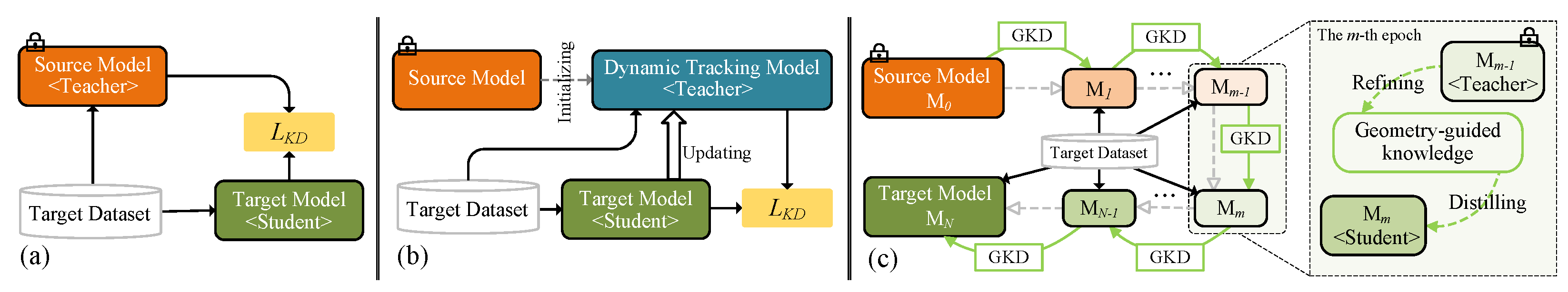
Most recently, knowledge distillation was applied regarding SFDA [16,17,18], and the adaptation was modeled as a knowledge transfer from the pre-trained source model (teacher model). These methods provided a natural solution for SFDA that is more in line with our cognitive experience. However, the existing methods did not carefully design the knowledge distillation skeleton to fit SFDA. First, the fixed source model is only in charge of predicting the semantic labels (Figure 1a), as conducted in [16,17]. The semantic supervision generated in this static way is also frozen during the whole transfer phase such that the power of the semantic guidance will gradually weaken, namely the semantic guidance degradation. Second, a dynamic tracking model, e.g., momentum network [18], was taken as the teacher model for conforming to the composition of a classic knowledge distillation framework (Figure 1b). Although this scheme solves the first problem above, the teacher model cannot well represent the semantic information to be transferred, namely semantic deviation, due to the semantic noise caused by the inherent discrepancy between the teacher model and the student model. Third, under the knowledge distillation framework, how to achieve better SFDA by exploiting the local geometry of target data is still an open problem.

Aiming at the limitations mentioned above, we develop a novel knowledge-distillation-based method for SFDA named Gradual Geometry-Guided Knowledge Distillation (G2KD). At the global level, G2KD slices the whole adaptation into a sequence of (N) stages/epochs, as shown in Figure 1c. There are two reasons for adopting this gradual strategy. First, it can resist the aforementioned semantic guidance degradation. Second, due to the model updating after each epoch, the data features change correspondingly, leading to variations in the local structure. Therefore, we need to construct the local structure for each epoch to realize knowledge distillation by this gradual strategy. At the epoch-level, inspired by the self-distillation methods [19,20], G2KD adopts the self-guided strategy to minimize the aforementioned semantic deviation. Specifically, the student model ${\mathrm{M}}_m$ shares the same structure with the teacher model ${\mathrm{M}}_{m-1}$ and is initiated by ${\mathrm{M}}_{m-1}$ at the beginning of the epoch. After that, for utilizing the local geometry, we adopt geometry-guided knowledge distillation (G2KD) to train ${\mathrm{M}}_m$. As shown in the right side of Figure 1c, G2KD works in a “refining–distilling” manner. Firstly, G2KD mines the geometry-guided knowledge by building local geometry of the neighborhood for any target data. Then, semantic fusion converts it to soft semantic supervision based on semantic estimation using k-means clustering and a teacher model’s output (refining). Secondly, G2KD performs knowledge distillation. In particular, we introduce an entropy loss with neighbor context for meeting the unsupervised requirement of SFDA (distilling).

Essentially, G2KD provides an implicit domain aligning approach without reliance on the source domain training data, as assumed in UDA, but only the need to access the pre-trained source model. To be concrete, the epoch-wise adaptation at the global level converts the large domain shift reduction, between the source domain (implicitly represented by the source model) and the target domain, into several successive easy tasks with a small shift. Furthermore, at the local (per-epoch) level, by integrating the local structure information based on the most discriminative up-to-date features (${\mathrm{M}}_{m-1}$), the obtained geometry-guided knowledge is more credible/accurate than the original outputs of ${\mathrm{M}}_{m-1}$. Empowered by the guidance of them, the performance of ${\mathrm{M}}_m$ can be enhanced further.

Our contributions cover the following three areas.

(1) We develop a novel gradual knowledge distillation framework G2KD for SFDA, exploiting the geometry-guided knowledge, i.e., the self-supervision dynamically mined from the target data’s local geometry, and a new entropy-regularized knowledge distillation method, G2KD. Unlike the existing distillation frameworks, it mitigates the problems of guidance degradation and guidance deviation.

(2) We propose a generation method for geometry-guided knowledge.

The data neighborhood, discovered by similarity comparison, is taken as the local geometry in our approach. Through semantic fusion based on semantic evaluation pre-obtained by both clustering and model outputs, the knowledge is generated.

(3) We carry out extensive experiments on four challenging datasets. The experiments show that our method achieves state-of-the-art results. In addition to the ablation study, we perform a careful investigation for analysis.

The remainder of the paper is organized as follows. Section 2 introduces the related work. Section 3 details the proposed method, followed by the experimental results and analyses in Section 4. Section 5 comprises the conclusion.

2. Related Work

2.1. Unsupervised Domain Adaptation

For UDA, the key is to reduce the domain drift. Since the source and target data are accessible during the transfer phase, probability matching becomes the main idea to solve this problem. Based on whether to use a deep learning algorithm, the current work in UDA can be divided into two categories: (1) deep-learning-based and (2) non-deep-learning-based. In the first category, researchers rely on techniques such as metric learning to reduce domain drift [2,21,22]. In these methods, an embedding space with a unified probability distribution was learnt by minimizing certain statistical measures, e.g., MMD (maximum mean discrepancy) [23], which were used to evaluate the discrepancy of the domains. In addition, adversarial learning has been another popular framework for its capability of aligning the probabilities of two different distributions [1,24,25]. The second category reduces the drift in diverse manners. From the geometric point of view, Gopalan et al. [26], Gong et al. [27], and Caseiro et al. [28] modeled the transfer process from the source domain to the target one by geodesic flow on a manifold of data. Focusing on energy, Tang et al. [29] developed an energy-distribution-based classifier by which confidence target data are detected. Pan et al. [30] and Zhang et al. [31] used the geometric relation between data at the global and nearest-neighbor scales, respectively. Chen et al. [32] introduced a style and semantic memory mechanism to address the domain generalization problem. In all the aforementioned methods, the source data are indispensable as labeled samples were used to explicitly formulate domain knowledge (e.g., probability, geometric structure, or energy). When the labeled data in the source domain are not available, these traditional UDA methods fail.

2.2. Source-Data-Free Domain Adaptation

The current solutions for this issue take one of three approaches. One focuses on mining transferable factors that are suitable for both domains. Tang et al. [33] supposed that a sample and its exemplar classifier (SVM) satisfy a certain mapping relationship. Following this idea, this method learnt the mapping on the source domain and predicted the classifier for each target sample to perform an individual classification. Tanwisuth et al. [34] mined transferable prototypes to boost the model adaptation. The second is concerned with converting model adaptation without source data to the classic UDA setting by faking a source domain. Li et al. [9] incorporated a conditional generative adversarial net to explore the potential of unlabeled target data. Du et al. [35] used source-hypothesis-based target data splitting to form the pseudo-source domain data. Tian et al. [11] combined source prototypes and Gaussian noise to generate a pseudo-source domain. The third performs self-training with a pre-trained source model to avoid the effects caused by the absence of a source domain and the label information of the target domain. Liang et al. [13] developed a general framework to implement an implicit alignment from the target data to the probability distribution of the source domain. In this method, information maximization and pseudo-labels were used to supervise self-training. Lao et al. [7] proposed a multi-hypothesis version. Yang et al. [15] performed a bi-alignment between the two groups where a classifier trained on the confidence group is used as self-supervision. All the methods achieved impressive results to some extent, but they ignored the fact that the essence of model adaptation in SFDA is a kind of knowledge extraction and transfer.

2.3. Self-Distillation Methods

In the traditional knowledge distillation framework, knowledge is transferred from the teacher network to the student network [36,37]. The teacher network often has been pre-trained on a large deep model, and the student network needs to be guided by the teacher network [38]. There is a special case in knowledge distillation. When the student network and the teacher network are the same model, we term it self-knowledge distillation (SKD) [39,40,41,42]. According to training characteristics, we can divide SKD into real-time self-knowledge distillation (RSKD) and progressive self-knowledge distillation (PSKD). Specifically, RSKD approaches focus on mining real-time knowledge, namely the knowledge from the current model to be trained, to conduct knowledge distillation. Zhang et al. [39] took the deep output of the entire neural network as real-time semantic knowledge to regulate the distillation for shallow network components. Yun et al. [40] proposed a class-wise self-knowledge distillation method that softens over-fitting predictions and reduces intra-class variation. To this purpose, the intra-class samples are used as the real-time knowledge for the distillation. PSKD methods achieve knowledge distillation by using the prediction from the history model as the knowledge for distillation. Yang et al. [41] proposed snapshot distillation, which extracts teacher knowledge from earlier epochs in the same generation to guide the later epoch of student learning. To further distill the knowledge in the deep neural network itself, Kim et al. [42] used the prediction of the model itself as teacher knowledge to enhance the generalization of the deep neural network instead of any other ways to augment the architecture or tune the hyper-parameters carefully. Combined with the above methods, we noticed that the previous method is not suitable for SFUDA as ground truth is required for all samples. Also, these methods did not put the knowledge hidden in the local geometry structure between data to good use.

3. Methodology

This section first formulates the SFDA problem and then presents the overview of G2KD. Following that, we present the components of our method in detail, respectively.

3.1. Source-Data-Free Domain Adaptation Problem Formulation

Given two different but related domains, i.e., source domain $\mathcal{S}$ and target domain $\mathcal{T}$, $\mathcal{S}$ contains $n_s$ labeled samples, while $\mathcal{T}$ has n unlabeled data. Both labeled and unlabeled samples share the same K categories. Let ${\mathcal{X}}_s={\left\{{\mathit{x}}_i^s\right\}}_{i=1}^{n_s}$ and ${\mathcal{Y}}_s={\left\{y_i^s\right\}}_{i=1}^{n_s}$ be the source samples and the corresponding labels, where $y_i^s$ is the label of ${\mathit{x}}_i^s$. Similarly, we denote the target samples and their labels by ${\mathcal{X}}_t=\{{\mathit{x}}_i{\}}_{i=1}^n$ and ${\mathcal{Y}}_t={\left\{y_i\right\}}_{i=1}^n$, respectively. Conventional UDA intends to conduct a K-way classification on the target domain, and the labeled source data and the unlabeled target data are both available as the cross-domain transfer process. In contrast, SFDA tries to build a target model $f_t:{\mathcal{X}}_t\to {\mathcal{Y}}_t$ for the same classification task, whilst only ${\mathcal{X}}_t$ and a source model $f_s:{\mathcal{X}}_s\to {\mathcal{Y}}_s$ pre-obtained on the source domain are available during the whole transfer process.

Remark 1.

In conventional UDA, the domain shift is expressed by the data from the two domains explicitly. In SFDA, as above, the source probability distribution is presented (parameterized) to the source model implicitly such that the shift is reflected in the classification accuracy of the source model on the target domain. Also, SFDA is a “white-box” case; that is, the pre-trained source model is accessible during the adaptation phase, and details, such as architecture and weight parameters, are known. In case the source model only outputs prediction and its details are absent, it is formulated to the topic named “black-box” source-data-free domain adaptation [43,44].

3.2. Approach Overview

This paper presents SFDA as a model adaptation consisting of sequential sub-transfers, as presented in Figure 1. Specifically, the whole adaptation from $f_s$ to $f_t$ is sliced to N epochs and learns an intermediate model in each epoch such that the domain shift might be reduced smoothly since the sequential sub-transfers can capture the dynamics in the adaptation process. Formally, we give this progressive process a simple form presented by

$$\begin{array}{cc}\hfill & {\mathrm{M}}_{m-1}\stackrel{\mathrm{G}2\mathrm{KD}}{\to }{\mathrm{M}}_m,m=1,2,\cdots ,N,\hfill \\ \hfill & with{\mathrm{M}}_0=f_s\mathrm{and}{\mathrm{M}}_N=f_t,\hfill \end{array}$$

(1)

where N is the maximal training epoch number, and notation $A\stackrel{\mathrm{G}2\mathrm{KD}}{\to }B$ denotes a single sub-transfer regulated by the G2KD method from model A to model B.

Without loss of generality, Figure 2 depicts any sub-transfer driven by G2KD, i.e., ${\mathrm{M}}_{m-1}\stackrel{\mathrm{G}2\mathrm{KD}}{\to }{\mathrm{M}}_m$. We can see that the sub-transfer contains two steps. Firstly, we initialize the current ${\mathrm{M}}_m$ by ${\mathrm{M}}_{m-1}$, which is trained in the last epoch and fixed during ${\mathrm{M}}_m$ training. Following this step, we train ${\mathrm{M}}_m$ by G2KD. In this design, ${\mathrm{M}}_m$ is the student model, while ${\mathrm{M}}_{m-1}$ is the teacher model. The transfer learning for ${\mathrm{M}}_m$ is driven by G2KD regularization (Figure 2b) consisting of three regulators: the entropy loss ${\mathcal{L}}_{\mathrm{ent}}$, distillation loss ${\mathcal{L}}_{\mathrm{dis}}$, and student loss ${\mathcal{L}}_{\mathrm{stu}}$. In the entropy loss, except for classic entropy minimization [45], we integrate the neighbor context of input instance. Another important component is the geometry-guided knowledge block (Figure 2a), which plays a central role in our distillation scheme. It provides the soft target and soft pseudo-label to supervise the distillation loss and student loss, respectively. Knowledge mining is achieved by local geometry discovery, which outputs the neighborhood geometry for the input instance. The followed knowledge representation transforms this knowledge into two supervision aspects, including a soft target and a soft pseudo-label. To this end, we perform semantic clustering and fusion based on the deep features and final outputs mapped by the teacher model ${\mathrm{M}}_{m-1}$, as shown in Figure 2c. In the following, we present these components in detail.

3.3. Structure of Intermediate Model ${\mathrm{M}}_m$

To account for classification in SFDA, the source model $f_s$ is divided into a feature extractor and a classifier, whose details are known according to the SFDA setting. In order to conduct the chain-like training starting with $f_s$, formulated by Equation (1), in the epoch-wise adaptation process of G2KD, all intermediate models ${\left\{{\mathrm{M}}_m\right\}}_{m=1}^N$ have the same structure as $f_s$. Specifically, we use a deep network to specify any intermediate model ${\mathrm{M}}_m$; ${\mathrm{M}}_m$ also consists of a feature extractor $e_m\left(·;{\theta }_m\right)$ and a classifier $c_m\left(·;{\psi }_m\right)$. Thus, ${\mathrm{M}}_m$ can be parameterized to $f_m=c_m\circ e_m\left(·;{\theta }_m,{\psi }_m\right)$, where $\{{\theta }_m,{\psi }_m\}$ collects the model parameters.

3.4. Geometry-Guided Knowledge

In this section, we first introduce the method to discover neighborhood representing the geometry-guided knowledge using the teacher model ${\mathrm{M}}_{m-1}$. Then, we present the semantic information extraction method to represent the mined knowledge regulating our knowledge distillation.

Knowledge mining. As mentioned above, we deem the local geometric relationship of any target data to be the knowledge. To implement this insight, we propose local geometry of the neighborhood to portray this relationship. The feature extractor in the teacher model maps all target samples ${\left\{{\mathit{x}}_i\right\}}_{i=1}^n$ to deep features ${\left\{{\overline{\mathit{z}}}_i\right\}}_{i=1}^n$, denoted by ${\overline{\mathcal{Z}}}_t$ collectively, where ${\overline{\mathit{z}}}_i=e_{m-1}\left({\mathit{x}}_i;{\theta }_{m-1}\right)$. We extract the knowledge from this deep feature space. 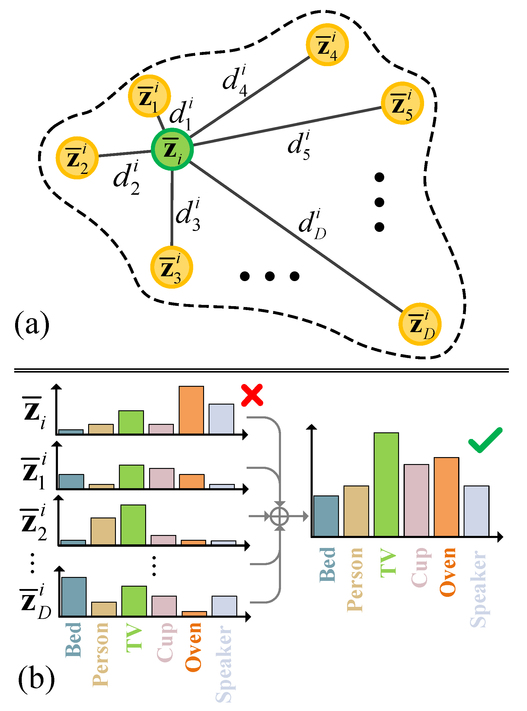Figure 3 presents the composition of this local structure, whose edge is marked by dotted line. The green circle located in the center stands for a feature sample of any target data, i.e., ${\overline{\mathit{z}}}_i$. The orange circles stand for D feature samples on the edge of the neighborhood, i.e., ${\left\{{\overline{\mathit{z}}}_j^i\right\}}_{j=1}^D$. In practice, we use the cosine similarity in the feature space to identify these neighbor samples ${\left\{{\overline{\mathit{z}}}_j^i\right\}}_{j=1}^D$. The similarities between the center sample and the edge samples are represented by the length of solid lines, i.e., ${\left\{d_j^i\right\}}_{j=1}^D$.

Obviously, if the constructing information ${\mathcal{I}}_i={\left\{({\overline{\mathit{z}}}_j^i,d_j^i)\right\}}_{j=1}^D$ is given, we can definitively determine the neighborhood of ${\overline{\mathit{z}}}_i$. We specify the neighborhood constructing information of any target sample ${\mathit{x}}_i$ by a simple strategy as follows. We first perform a similarity comparison of ${\mathit{x}}_i$ over the whole target dataset in the deep space and obtain a similarity measure set $\mathcal{A}=\left\{d_i\left|d_i=\phi ({\overline{\mathit{z}}}_i,{\overline{\mathit{z}}}_j),{\overline{\mathit{z}}}_j\in {\overline{\mathcal{Z}}}_t\right.\right\}$, where function $\phi ({\mathit{x}}_1,{\mathit{x}}_2)$ calculates the cosine similarity of ${\mathit{x}}_1$ and ${\mathit{x}}_2$. After that, we choose D feature samples closest to ${\overline{\mathit{z}}}_i$ and the corresponding distance (the similarity measure value) to form the neighborhood structure. This operation can be formulated by

$$\begin{array}{c}\hfill {\mathcal{I}}_i=\left\{\left({\overline{\mathit{z}}}_j^i,d_j^i\right)\left|{\overline{\mathit{z}}}_j^i\in {\overline{\mathcal{Z}}}_t,d_j^i\in \mathcal{A},j\in \mathrm{topk}\left(\mathcal{A},D\right)\right.\right\},\end{array}$$

(2)

where function $\mathrm{topk}(\mathcal{X},m)$ returns the indices of elements ranking in the first m in set $\mathcal{X}$.

Knowledge representing. By the above discovery method, we mine the knowledge from the teacher model. However, this knowledge cannot directly support the knowledge distillation. We therefore need to convert it to semantic information compatible with knowledge distillation learning. Corresponding to classic knowledge distillation, we propose (1) soft target and (2) soft pseudo-label to supervise the distillation loss and the student loss for the student model. The generation methods of them are presented in the remainder of this sub-section.

(1) Soft target. Unlike the classic distillation method that directly takes the teacher model’s output as the knowledge to guide the student learning, we use the soft target building on the constructed neighborhood to supervise the distillation part. Suppose ${\overline{\mathit{p}}}_i$ and ${\left\{{\overline{\mathit{p}}}_j^i\right\}}_{j=1}^D$ are the probability vectors of ${\overline{\mathit{z}}}_i$ and ${\left\{{\overline{\mathit{z}}}_j^i\right\}}_{j=1}^D$, respectively, under the mapping of $\mathrm{softmax}\left(c_{m-1}(·,{\psi }_{m-1})\right)$. Equation (3) formulates our construction procedure.

$$\begin{array}{c}\hfill {\overline{\mathit{o}}}_i={\overline{\mathit{p}}}_i+\sum _{j=1}^D{d}_j^i{\overline{\mathit{p}}}_j^i.\end{array}$$

(3)

(2) Soft pseudo-label. In classic knowledge distillation, the student loss is used to regulate the supervision learning on the given ground truth. However, due to the unavailable truth labels in SFDA, we use pseudo-labels instead. Moreover, we soften pseudo-labels to enhance knowledge transfer by absorbing the semantic information hidden in the neighborhood. To this end, we first extract essential semantic representation through cluster-based classification, the same as [13], and then perform semantic fusion based on the discovered local geometry. This process includes the following three steps.

(1) Weighted k-means clustering. For the deep features ${\left\{{\overline{\mathit{z}}}_i\right\}}_{i=1}^n$, the teacher model ${\mathrm{M}}_{m-1}$ predicts, after the Softmax operation, the probability vectors ${\left\{{\overline{\mathit{p}}}_i\right\}}_{i=1}^n$, where ${\overline{\mathit{p}}}_i=\mathrm{softmax}\left(c_{m-1}({\overline{\mathit{z}}}_i,{\psi }_{m-1})\right)$. We find the k-th cluster centroid by Equation (4), where ${\overline{p}}_{i,k}$ is the k-th element of vector ${\overline{\mathit{p}}}_i$.

$${\nu }_k={\displaystyle \frac{{\sum }_{i=1}^{n_t}{\overline{p}}_{i,k}{\overline{\mathit{z}}}_i}{{\sum }_{i=1}^{n_t}{\overline{p}}_{i,k}}}.$$

(4)

(2) Semantic extraction. We obtain the hard pseudo-labels of all feature samples constructing the neighborhood, including ${\overline{\mathit{z}}}_i$ and ${\left\{{\overline{\mathit{z}}}_j^i\right\}}_{j=1}^D$, using max-similarity-based classification formulated by Equation (5), where $\phi (·,·)$ is also a cosine similarity function, and D is the number of neighbor features.

$$\begin{array}{cc}\hfill {\overline{y}}_i& =arg\underset{k}{max}\phi ({\overline{\mathit{z}}}_i,{\nu }_k),\hfill \\ \hfill {\overline{y}}_j^i& =arg\underset{k}{max}\phi ({\overline{\mathit{z}}}_j^i,{\nu }_k),j=1,2,\cdots ,D.\hfill \end{array}$$

(5)

(3) Semantic fusion. Let ${\overline{\mathit{l}}}_i$ be the soft pseudo-label of any target data ${\mathit{x}}_i^t$; we formulate its generation by Equation (6), where ${\overline{\mathit{l}}}_{i,k}$ is the k-th element of ${\overline{\mathit{l}}}_i$, $\mathrm{I}[·]$ is the function of the indicator, ${\left\{d_j^i\right\}}_{j=1}^D$ is pre-obtained as we model adaptation knowledge via the neighborhood geometry, and K is the number of categories shared by the source and target domains.

$$\begin{array}{c}\hfill {\overline{\mathit{l}}}_{i,k}=\mathrm{I}\left[k={\overline{y}}_i\right]+\sum _{j=1}^D\sum _{k=1}^K{d}_j^i\mathrm{I}\left[k={\overline{y}}_j^i\right].\end{array}$$

(6)

3.5. Geometry-Guided Knowledge Distillation Regularization

Our knowledge distillation is a particular case of self-distillation since, at the beginning of each training epoch, we use the historical model pre-trained in the latest epoch to accomplish knowledge mining in the current epoch. Its objective also consists of two components, the distillation loss and the student loss, as in most previous work on knowledge distillation. However, compared with this other work, our regularization builds on the semantic information mined from the geometry-guided knowledge.

I. Entropy regulator with neighbor context

Entropy-based regularization is widely used in unsupervised classification scenarios [46,47], leading to the aggregation of samples without semantic supervision. However, this aggregation only relying on model’s prediction will amplify the prediction errors in a positive feedback way. Therefore, the single use of entropy minimization is always regulated further. In this work, we develop entropy minimization with neighbor relation, focusing on utilizing geometry-based semantic context. In the absence of real supervision in the SFDA setting, the semantic relations between these neighbor samples are not reliable. To bypass this limitation, we take the augmentation data with a slight transformation as the neighbor. Thus, we can use the category consistency constraint on the data before and after augmentation to enhance feature discrimination. To this end, in addition to the classic entropy item, we introduce another entropy regulator [48], which maximizes the mutual information entropy between the input instance and its augmentation data.

During the m-th training epoch, given any input instance ${\mathit{x}}_i$ and its augmentation data ${\mathit{x}}_i^{\prime }$, obtained by rotating ${\mathit{x}}_i$ with a small angle selected from $[-\delta ,\delta ]$ randomly, ${\mathrm{M}}_m$ converts ${\mathit{x}}_i$ and ${\mathit{x}}_i^{\prime }$ to probability vectors ${\mathit{p}}_i$ and ${\mathit{p}}_i^{\prime }$ over all classes, respectively. The proposed entropy loss on the instance ${\mathit{x}}_i$ can be expressed by

$${\mathcal{L}}_e=H\left({\mathit{p}}_i\right)-\alpha I\left({\mathit{p}}_i,{\mathit{p}}_i^{\prime }\right).$$

(7)

where $H\left({\mathit{p}}_i\right)=-{\sum }_{k=1}^K{p}_{i,k}log{p}_{i,k}$ is the entropy measure; $I(·,·)$ is the mutual information measure [49] whose computation is the same as [48]; $\alpha$ is a trade-off hyper-parameter. In this equation, the first term is the classic entropy minimization loss to regulate the individual data. The second term introduces the semantic constraint in the augmentation-based neighbor context for discriminative features.

II. Knowledge distillation regulator

With the notation mentioned above, corresponding to the input instance ${\mathit{x}}_i$, its logit is ${\mathit{r}}_i$, which is mapped through the student model. Using the temperature Softmax formulated by Equation (8) where $T>0$ is the temperature scaling parameter, we map ${\mathit{r}}_i$ to the soft target ${\mathit{p}}_i^{\prime }$.

$$\begin{array}{c}\hfill p_{i,k}^{\prime }={\displaystyle \frac{exp(q_{i,k}/T)}{{\sum }_{j=1}^{K}exp(q_{i,j}/T)}}.\end{array}$$

(8)

Combining the soft target in Equation (3), we express the distillation loss in the form of the Kullback–Leibler (KL) divergence

$$\begin{array}{cc}\hfill {\mathcal{L}}_{\mathrm{dis}}& =\mathrm{KL}\left({\overline{\mathit{o}}}_i\left|\right|{\mathit{p}}_i^{\prime }\right)\hfill \\ \hfill & =-{\displaystyle \frac{1}{n}}\sum _{i=1}^n\sum _{k=1}^K{\overline{o}}_{i,k}log{\displaystyle \frac{{\overline{o}}_{i,k}}{p_{i,k}^{\prime }}}.\hfill \end{array}$$

(9)

Combining the soft pseudo-label in Equation (6), we express the student loss by Equation (10), where ${\varrho }_k={\displaystyle \frac{1}{n_t}}{\sum }_{i=1}^{n_t}{p}_{i,k}$ is a mean in the k-th dimension over all target data. In this loss, the first term in cross-entropy form is similar to the classic student loss used in the traditional knowledge distillation framework. The difference between them is that we replace the ground truth by our constructed soft pseudo-label. Due to the errors in the pseudo-labels, the first regularization cannot guide semantic learning absolutely correctly. To relieve the negative impact from the pseudo-labels, like [13,50,51], we introduce the category balance loss as the second regularization term. The $\beta$ and $\gamma$ are hyper-parameters.

$$\begin{array}{c}\hfill {\mathcal{L}}_{\mathrm{stu}}=-\beta {\displaystyle \frac{1}{n}}\sum _{i=1}^n\sum _{k=1}^K{\overline{l}}_{i,k}log{p}_{i,k}+\gamma \sum _{k=1}^K{\varrho }_{k}log{\varrho }_k.\end{array}$$

(10)

Thus, we have the following loss with knowledge-distillation-like structure.

$$\begin{array}{c}\hfill {\mathcal{L}}_{\mathrm{kd}}={\mathcal{L}}_{\mathrm{dis}}+{\mathcal{L}}_{\mathrm{stu}}.\end{array}$$

(11)

Based on the regularizers represented in Equations (7) and (11), we have our final objective for the G2KD method

$$\begin{array}{c}\hfill \underset{\{{\theta }_m,{\psi }_m\}}{min}{\mathcal{L}}_{\mathrm{G}2\mathrm{KD}}={\mathcal{L}}_{\mathrm{ent}}+{\mathcal{L}}_{\mathrm{kd}}.\end{array}$$

(12)

3.6. Model Training

Algorithm 1 summarizes the training overview for the model adaptation from $f_s$ to $f_t$ based on G2KD.

Algorithm 1 Overall training of G2KD

Input: The trained source model $f_s$, target data ${\mathcal{X}}_t$, max epoch number N, iteration number of each epoch $I_e$. Output: The target model $f_t={\mathrm{M}}_N$.  1: Let ${\mathrm{M}}_{m-1}={\mathrm{M}}_0=f_s$.  2: for epoch-index = 1 to N do  3:  Initialize the student model ${\mathrm{M}}_m$ by the trained teacher model ${\mathrm{M}}_{m-1}$, i.e., $\{{\theta }_m,{\psi }_m\}=\{{\theta }_{m-1},{\psi }_{m-1}\}$.  4:  Refine geometry-guided knowledge, i.e., local geometry, by teacher model ${\mathrm{M}}_{m-1}$ according to Equation (2).  5:  for iter-index = 1 to $I_e$ do  6:   Sample a mini-batch from ${\mathcal{X}}_t$.  7:   Generate soft target for this batch by Equation (3).  8:   Generate soft pseudo-label for this batch by Equation (6).  9:   Update $\{{\theta }_m,{\psi }_m\}+=\Delta {\mathcal{L}}_{\mathrm{G}2\mathrm{KD}}$, where the objective is represented by Equation (12).  10:  end for  11: end for  12: return: ${\mathrm{M}}_N$.

4. Experiments and Analyses

This section first provides the experimental settings, including the dataset introduction, details on implementation, and the baseline for comparison. After that, experimental results on four benchmarks are presented, followed by an analysis and ablation study, respectively.

4.1. Datasets

In this paper, we evaluate G2KD on four widely used benchmarks, i.e., Office-31, Office-Home, VisDA and DomainNet. Among them, Office-31 and VisDA are only used for the task of vanilla closed-set domain adaptation, whilst Office-Home and DomainNet are adopted for both vanilla closed-set domain adaptation tasks and multi-source-domain adaptation tasks.

Office-31 [52]. Office-31 is a small-scale dataset that is widely used in visual domain adaptation including three domains, i.e., Amazon (A), Webcam (W), and Dslr (D), all of which are taken from real-world objects in various office environments. The dataset has 4652 images of 31 categories in total. Images in (A) are online e-commerce pictures. (W) and (D) consist of low-resolution and high-resolution pictures.

Office-Home [53]. Office-Home is a medium-scale dataset that is mainly used for domain adaptation, containing 15,000 images belonging to 65 categories from working or family environments. The dataset has four distinct domains, i.e., artistic images (Ar), clip art (Cl), product images (Pr), and real-world images (Rw).

VisDA [54]. VisDA is a challenging large-scale dataset with 12 types of synthetic to real transfer recognition tasks. The source domain contains 152,000 synthetic images, while the target domain has 55,000 real object images from Microsoft COCO.

DomainNet [55]. DomainNet is the most challenging large-scale dataset, with 0.6 million images of 345 classes from 6 domains of different image styles: clip art (C), infograph (I), painting (P), quickdraw (Q), real (R), and sketch (S).

4.2. Implementation Details

Network structure. We design and implement our network architecture based on Pytorch. We can divide the above datasets into two types, vanilla closed-domain adaptation and multi-source-domain adaptation, for the vanilla closed-set domain adaptation task. In our model, the feature extractor contains a heavy-weight deep architecture and a compression layer consisting of a batch-normalization layer and a full-connect layer with a size of 2048 × 256. Specifically, for the deep architecture, like [2,18,56], we use ResNet-50 pre-trained on ImageNet as the feature extractor in the experiments on Office-31, Office-Home, and DomainNet. At the same time, on VisDA, we adopt ResNet-101 to replace ResNet-50 used in the methods without the VIT module, whilst methods with VIT, i.e., TDA, SHOT + VIT, and G2KD + VIT, still keep ResNet-50 as the backbone. The classifier consists of a weight-normalization layer and a full-connect layer with a size of 256 × K, in which K differs from one dataset to another.

Source model training. For all evaluation datasets, the source model $f_s$ was pre-trained with the standard protocol [7,8,13,15]. We split the labeled source data into two parts of 90%:10% for model pre-training and validation.We set the training epochs on Office-31, Office-Home, VisDA, and DomainNet to 100, 50, 10, and 20, respectively.

Parameter settings. For Office-31, Office-Home, and DomainNet, we set the learning rate and epochs to 0.01 and 15, respectively; for VisDA, the learning rate is set to 0.001 and the same epochs. For hyper-parameters, we set $\delta =10$, $D=4$, $\alpha =0.1$, $\beta =0.05$, and $\gamma =0.8$. Additionally, the batch size for all tasks is set to 64. All the experiments were run on a single GPU of NVIDIA RTX TITAN.

4.3. Competitors

To verify the effectiveness of our method, we select 24 competing methods in three groups, as shown below.

(1)

The first group includes two deep models, i.e., ResNet-50 and ResNet-101 [57]. They are used to initiate the feature extractor of the source model.

(2)

The second group includes 12 current state-of-the-art UDA methods with access to the source data. They are CDAN [2], SWD [58], DMRL [59], BSP [60], TN [61], TPN [22], IA [62], BNM [63], MCC [64], A2LP [31], CGDM [65], CaCo [66], SUDA [67], ${\mathrm{SImpAI}}_{50}$ [68], CMSDA [69], DRT [70], and STEM [71].

(3)

The third group includes 10 current state-of-the-art SFDA methods. They are SFDA [10], 3C-GAN [9], SHOT [13], BAIT [15], HMI [7], PCT [34], GPGA [8], AAA [12], PS [35], VDM [11], DECISION [72], NRC [73], and GKD [74].

To extensively evaluate G2KD, we further introduce two variants: G2KD++ and G2KD + ViT. Specifically, G2KD++ is an enhanced version with semi-supervised learning (MixMatch) [75], whilst SHOT + ViT is a feature-empowered version with a VIT module [76]. For comparison, SHOT++ [77], SHOT + ViT, and TDA [18] are adopted as the baselines, where SHOT++ and SHOT + ViT are implemented in the same way to G2KD++ and G2KD + ViT, respectively. In practice, these methods with ViT, SHOT + ViT, TDA, and G2KD+ViT implement the feature extractor using ResNet50 + ViT instead of ResNet50 (on Office-31, Office-Home, and DomainNet) and ResNet101 (on VisDA), adopted in SHOT and G2KD. We inject the transformer layer, similar to [18], between the ResNet-50 architecture and the compression layer.

4.4. Quantitative Results

Vanilla closed-set domain adaptation.

Table 1. Classification accuracies (%) on the Office-31 dataset for vanilla closed-set DA based on ResNet50 backbone. SF means source-data-free, blue bold means best results without both MixMatch and ViT, and green and orange bold mean best results empowered by MixMatch and ViT, respectively.

Method/Task	SF	A→D	A→W	D→A	D→W	W→A	W→D	Avg.
ResNet50 [57]	✗	68.9	68.4	62.5	96.7	60.7	99.3	76.1
CDAN [2]	✗	92.9	94.1	71.0	98.6	69.3	100.0	87.7
BSP [60]	✗	93.0	93.3	73.6	98.2	72.6	100.0	88.5
TN [61]	✗	94.0	95.0	73.4	98.7	74.2	100.0	89.3
DMRL [59]	✗	93.4	90.8	73.0	99.0	71.2	100.0	87.9
IA [62]	✗	92.1	90.3	75.3	98.7	74.9	99.8	88.8
BNM [63]	✗	90.3	91.5	70.9	98.5	71.6	100.0	87.1
MCC [64]	✗	95.6	95.4	72.6	98.6	73.9	100.0	89.4
A2LP [31]	✗	87.8	87.7	75.8	98.1	75.9	98.1	87.4
CaCo [66]	✗	91.7	89.7	73.1	98.4	72.8	100.0	87.6
SUDA [67]	✗	91.2	90.8	72.2	98.7	71.4	100.0	87.4
SFDA [10]	✓	92.2	91.1	71.0	98.2	71.2	99.5	87.2
3C-GAN [9]	✓	92.7	93.7	75.3	98.5	77.8	99.8	89.6
SHOT [13]	✓	93.9	91.3	74.1	98.2	74.6	100.0	88.7
BAIT [15]	✓	92.0	94.6	74.6	98.1	75.2	100.0	89.1
HMI [7]	✓	94.4	94.0	73.7	98.9	75.9	99.8	89.5
PCT [34]	✓	–	–	–	–	–	–	88.4
CPGA [8]	✓	94.4	94.1	76.0	98.4	76.6	98.4	89.9
AAA [12]	✓	95.6	94.2	75.6	98.1	76.0	99.8	89.9
VDM [11]	✓	94.1	93.2	75.8	98.0	77.1	100.0	89.7
NRC [73]	✓	96.0	90.8	75.3	99.0	75.0	100.0	89.4
GKD [74]	✓	94.6	91.6	75.1	98.7	75.1	100.0	89.2
Source-model-only	✓	79.9	75.9	58.7	94.5	63.6	98.4	78.5
G2KD (ours)	✓	96.1	94.3	75.5	98.6	75.3	100.0	90.0
SHOT++ [77]	✓	95.2	91.2	74.7	98.6	75.4	100.0	89.2
G2KD++ (ours)	✓	96.7	94.5	76.0	98.7	75.7	100.0	90.2
TDA [18]	✓	97.2	95.0	73.7	99.3	79.3	99.6	90.7
SHOT + ViT	✓	98.4	96.4	80.9	98.3	83.5	100.0	93.0
G2KD + ViT (ours)	✓	98.2	95.4	81.9	99.1	84.6	99.8	93.2

,

Table 2. Classification accuracies (%) on the Office-Home dataset for vanilla closed-set DA based on ResNet50 backbone. SF means source-data-free, blue bold means best results without both MixMatch and ViT, and green and orange bold mean best results empowered by MixMatch and ViT, respectively.

Method/Task	SF	Ar→Cl	Ar→Pr	Ar→Rw	Cl→Ar	Cl→Pr	Cl→Rw	Pr→Ar	Pr→Cl	Pr→Rw	Rw→Ar	Rw→Cl	Rw→Pr	Avg.
ResNet-50 [57]	✗	34.9	50.0	58.0	37.4	41.9	46.2	38.5	31.2	60.4	53.9	41.2	59.9	46.1
CDAN [2]	✗	50.7	70.6	76.0	57.6	70.0	70.0	57.4	50.9	77.3	70.9	56.7	81.6	65.8
BSP [60]	✗	52.0	68.6	76.1	58.0	70.3	70.2	58.6	50.2	77.6	72.2	59.3	81.9	66.3
TN [61]	✗	50.2	71.4	77.4	59.3	72.7	73.1	61.0	53.1	79.5	71.9	59.0	82.9	67.6
IA [62]	✗	56.0	77.9	79.2	64.4	73.1	74.4	64.2	54.2	79.9	71.2	58.1	83.1	69.5
BNM [63]	✗	52.3	73.9	80.0	63.3	72.9	74.9	61.7	49.5	79.7	70.5	53.6	82.2	67.9
SFDA [10]	✓	48.4	73.4	76.9	64.3	69.8	71.7	62.7	45.3	76.6	69.8	50.5	79.0	65.7
SHOT [13]	✓	56.6	78.0	80.6	68.4	78.1	79.4	68.0	54.3	82.2	74.3	58.7	84.5	71.8
BAIT [15]	✓	57.4	77.5	82.4	68.0	77.2	75.1	67.1	55.5	81.9	73.9	59.5	84.2	71.6
HMI [7]	✓	57.8	76.7	81.9	67.1	78.8	78.8	66.6	55.5	82.4	73.6	59.7	84.0	71.9
PCT [34]	✓	–	–	–	–	–	–	–	–	–	–	–	–	71.0
CPGA [8]	✓	59.3	78.1	79.8	65.4	75.5	76.4	65.7	58.0	81.0	72.0	64.4	83.3	71.6
AAA [12]	✓	56.7	78.3	82.1	66.4	78.5	79.4	67.6	53.5	81.6	74.5	58.4	84.1	71.8
PS [35]	✓	57.8	77.3	81.2	68.4	76.9	78.1	67.8	57.3	82.1	75.2	59.1	83.4	72.1
VDM [11]	✓	59.3	75.3	78.3	67.6	76.0	75.9	68.8	57.7	79.6	74.0	61.1	83.6	71.4
NRC [73]	✓	57.7	80.3	82.0	68.1	79.8	78.6	65.3	56.4	83.0	71.0	58.6	85.6	72.2
GKD [74]	✓	56.5	78.2	81.8	68.7	78.9	79.1	67.6	54.8	82.6	74.4	58.5	84.8	72.2
Source-model-only	✓	44.3	67.0	73.7	52.5	62.5	64.6	51.5	40.6	72.0	65.6	46.4	72.2	59.4
G2KD (ours)	✓	56.9	79.2	81.6	68.2	79.5	80.1	68.0	56.2	82.4	74.5	59.3	84.6	72.5
SHOT++ [77]	✓	57.3	78.9	81.5	69.4	79.7	80.6	68.4	55.1	82.5	75.2	60.1	84.9	72.8
G2KD++ (ours)	✓	57.4	79.8	82.3	68.9	80.2	80.6	68.1	56.6	82.5	74.8	59.4	84.9	73.0
TDA [18]	✓	67.5	83.3	85.9	74.0	83.8	84.4	77.0	68.0	87.0	80.5	69.9	90.0	79.3
SHOT + ViT	✓	71.2	87.2	87.4	79.1	87.8	87.6	80.0	70.6	88.7	82.1	72.4	91.1	82.1
G2KD + ViT (ours)	✓	72.8	87.9	88.4	80.1	88.3	88.8	81.1	71.9	89.2	82.4	73.9	90.7	83.0

and

Table 3. Classification accuracies (%) on the VisDA dataset for vanilla closed-set DA. SF means source-data-free, blue bold means best results without both MixMatch and ViT, and green and orange bold mean best results empowered by MixMatch and ViT, respectively. The methods with ViT adopt the backbone of ResNet50, whilst other methods use the ResNet101 backbone.

Method/Class	SF	Plane	Bcycl	Bus	Car	Horse	Knife	Mcycl	Person	Plant	Sktbrd	Train	Truck	Per-Class
ResNet-101 [57]	✗	55.1	53.3	61.9	59.1	80.6	17.9	79.7	31.2	81.0	26.5	73.5	8.5	52.4
CDAN [2]	✗	85.2	66.9	83.0	50.8	84.2	74.9	88.1	74.5	83.4	76.0	81.9	38.0	73.9
BSP [60]	✗	92.4	61.0	81.0	57.5	89.0	80.6	90.1	77.0	84.2	77.9	82.1	38.4	75.9
SWD [58]	✗	90.8	82.5	81.7	70.5	91.7	69.5	86.3	77.5	87.4	63.6	85.6	29.2	76.4
TPN [22]	✗	93.7	85.1	69.2	81.6	93.5	61.9	89.3	81.4	93.5	81.6	84.5	49.9	80.4
IA [62]	✗	-	-	-	-	-	-	-	-	-	-	-	-	75.8
DMRL [59]	✗	-	-	-	-	-	-	-	-	-	-	-	-	75.5
A2LP [31]	✗	-	-	-	-	-	-	-	-	-	-	-	-	82.7
MCC [64]	✗	88.7	80.3	80.5	71.5	90.1	93.2	85.0	71.6	89.4	73.8	85.0	36.9	78.8
CaCo [66]	✗	90.4	80.7	78.8	57.0	88.9	87.0	81.3	79.4	88.7	88.1	86.8	63.9	80.9
SUDA [67]	✗	88.3	79.3	66.2	64.7	87.4	80.1	85.9	78.3	86.3	87.5	78.8	74.5	79.8
CGDM [65]	✗	93.4	82.7	73.2	68.4	92.9	94.5	88.7	82.1	93.4	82.5	86.8	49.2	82.3
SFDA [10]	✓	86.9	81.7	84.6	63.9	93.1	91.4	86.6	71.9	84.5	58.2	74.5	42.7	76.7
SHOT [13]	✓	95.0	87.4	81.0	57.6	93.9	94.0	79.5	80.4	90.9	89.9	85.9	57.4	82.7
3C-GAN [9]	✓	94.8	73.4	68.8	74.8	93.1	95.4	88.6	84.7	89.1	84.7	83.5	48.1	81.6
BAIT [15]	✓	93.7	83.2	84.5	65.0	92.9	95.4	88.1	80.8	90.0	89.0	84.0	45.3	82.7
HMI [7]	✓	-	-	-	-	-	-	-	-	-	-	-	-	82.4
CPGA [8]	✓	94.8	83.6	79.7	65.1	92.5	94.7	90.1	82.4	88.8	88.0	88.9	60.1	84.1
AAA [12]	✓	94.4	85.9	74.9	60.2	96.0	93.5	87.8	80.8	90.2	92.0	86.6	68.3	84.2
PS [35]	✓	95.3	86.2	82.3	61.6	93.3	95.7	86.7	80.4	91.6	90.9	86.0	59.5	84.1
VDM [11]	✓	96.9	89.1	79.1	66.5	95.7	96.8	85.4	83.3	96.0	86.6	89.5	56.3	85.1
NRC [73]	✗	96.8	91.3	82.4	62.4	96.2	95.9	86.1	90.7	94.8	94.1	90.4	59.7	85.1
GKD [74]	✗	95.3	87.6	81.7	58.1	93.9	94.0	80.0	80.0	91.2	91.0	86.9	56.1	83.0
Source-model-only	✓	74.9	18.4	48.4	68.6	70.0	7.0	85.3	33.2	81.4	33.6	86.6	8.0	51.2
G2KD (ours)	✓	96.0	89.1	83.5	65.6	95.0	96.0	86.9	82.4	92.2	92.2	90.8	54.9	85.4
SHOT++ [77]	✓	97.2	87.6	87.1	75.2	96.5	97.8	92.1	84.4	96.9	89.7	93.7	36.4	86.2
G2KD++ (ours)	✓	97.3	88.5	89.8	74.9	97.4	98.4	91.7	79.6	96.3	91.9	93.9	40.6	86.7
TDA [18]	✓	96.6	90.6	86.3	45.1	93.1	96.1	70.7	54.4	85.8	92.2	93.0	51.7	79.6
SHOT + ViT	✓	97.5	91.6	86.2	46.8	96.7	92.0	76.3	72.7	94.7	94.8	92.8	54.2	83.0
G2KD + ViT (ours)	✓	97.8	93.3	91.8	61.4	98.1	97.1	87.5	73.4	96.8	97.1	94.3	53.3	86.8

present the experimental results of the object recognition. On the Office-31 dataset (see Table 1), among these methods without extending, namely saving SHOT++, TDA, and SHOT+VIT, G2KD obtains the best results on the tasks A→D and W→D. Compared with the previous best method, GPGA and AAA, G2KD improves 0.1% on average due to the gap of 1.3% on task W→A, along with slight improvement on other tasks. For the methods with MixMatch, G2KD++ beats SHOT++ on all tasks, improving by 1.0% in average accuracy. For the ViT methods, G2KD + ViT obtains the best results in half tasks. In average accuracy, G2KD + ViT improves by 0.2% as opposed to the second-best method, SHOT + ViT.

On the Office-Home dataset (see Table 2), in the method group without MixMatch and ViT, G2KD obtains the best results on half tasks and improves 0.3% in average accuracy compared with the second-best method, NRC and GKD. When MixMatch and ViT are introduced, the performance of our method further improves. G2KD++ surpasses SHOT++ in 8 out of 12 tasks, whilst G2KD + ViT achieves the best results in 10 out of 12 tasks. Correspondingly, G2KD++ and G2KD + VIT improve the average accuracy by 0.2% and 0.9%, respectively, over the second-best method, SHOT++ and SHOT + VIT.

On the VisDA dataset (see Table 3), G2KD achieves the best results in three classes, “skrbrd” and “train’,’ and beats the second-best method, VDM and NRC, by a 0.3% improvement on average. With semi-supervised learning, G2KD++ obtains the best results on 8 out of 12 tasks compared to SHOT++, leading to 0.5% increase in average accuracy. As for the ViT-based methods, the advantages of our method become more evident. G2KD + ViT ranks first in average accuracy, with the best results regarding 10 out of 12 classes. It improves by 3.8% in average accuracy compared to the second-best method, SHOT + ViT.

From Table 1 to Table 3, the extensive versions of G2KD, i.e., G2KD++ and G2KD + VIT, defeat other methods, including G2KD. It indicates that both semi-supervised learning and stronger features can boost our method further. From Office-31 to VisDA, G2KD++ surpasses G2KD by 0.7% on average, whilst SHOT++ surpasses SHOT by 1.7% on average. In contrast, on the same three datasets, both G2KD + ViT and SHOT + ViT beat G2KD and SHOT by 5.0% on average. These results show that enhancing feature extraction is a better choice for elevating G2KD compared with semi-supervised learning.

On the most challenging large-scale dataset, Domain-Net (see

Table 4. Classification accuracies (%) on the Domain-Net dataset for vanilla closed-set DA. Blue bold means best result. Works marked with “*” are source-data-free domain adaptation methods. In the six sub-tables, each row reports the adaptation results from one source domain to the other five target domains.

CDAN	C	I	P	Q	R	S	Avg.	BNM	C	I	P	Q	R	S	Avg.	SWD	C	I	P	Q	R	S	Avg.
C	–	13.5	28.3	9.3	43.8	30.2	25.0	C	–	12.1	33.1	6.2	50.8	40.2	28.5	C	–	14.7	31.9	10.1	45.3	36.5	27.7
I	18.9	–	21.4	1.9	36.3	21.3	20.0	I	26.6	–	28.5	2.4	38.5	18.1	22.8	I	22.9	–	24.2	2.5	33.2	21.3	20.0
P	29.6	14.4	–	4.1	45.2	27.4	24.2	P	39.9	12.4	–	3.4	54.5	36.2	29.2	P	33.6	15.3	–	4.4	46.1	30.7	26.0
Q	11.8	1.2	4.0	–	9.4	9.5	7.2	Q	17.8	1.0	3.6	–	9.2	8.3	8.0	Q	15.5	2.2	6.4	–	11.1	10.2	9.1
R	36.4	18.3	40.9	3.4	–	24.6	24.7	R	48.6	13.2	49.7	3.6	–	33.9	29.8	R	41.2	18.1	44.2	4.6	–	31.6	27.9
S	38.2	14.7	33.9	7.0	36.6	–	26.1	S	54.9	12.8	42.3	5.4	51.3	–	33.3	S	44.2	15.2	37.3	10.3	44.7	–	30.3
Avg.	27.0	12.4	25.7	5.1	34.3	22.6	21.2	Avg.	37.6	10.3	31.4	4.2	40.9	27.3	25.3	Avg.	31.5	13.1	28.8	6.4	36.1	26.1	23.6
CGDM	C	I	P	Q	R	S	Avg.	SHOT *	C	I	P	Q	R	S	Avg.	G2KD *	C	I	P	Q	R	S	Avg.
C	–	16.9	35.3	10.8	53.5	36.9	30.7	C	–	16.3	42.4	14.4	48.0	27.9	29.8	C	–	17.8	45.5	16.0	65.5	47.7	38.3
I	27.8	–	28.2	4.4	48.2	22.5	26.2	I	26.0	–	25.5	5.9	43.6	16.4	23.5	I	46.7	–	42.8	4.8	62.3	36.3	38.6
P	37.7	14.5	–	4.6	59.4	33.5	30.0	P	32.3	7.7	–	7.3	48.0	24.5	24.0	P	55.5	19.1	–	7.6	66.6	44.2	38.6
Q	14.9	1.5	6.2	–	10.9	10.2	8.7	Q	20.6	2.0	6.0	–	5.9	12.3	9.3	Q	18.1	1.4	6.8	–	5.6	13.0	9.0
R	49.4	20.8	47.2	4.8	–	38.2	32.0	R	57.0	20.7	49.5	5.9	–	43.3	35.3	R	59.6	21.5	51.9	9.5	–	45.5	37.6
S	50.1	16.5	43.7	11.1	55.6	–	35.4	S	57.4	16.7	43.9	16.1	60.2	–	38.9	S	60.1	17.4	47.8	18.0	64.9	–	41.6
Avg.	36.0	14.0	32.1	7.1	45.5	28.3	27.2	Avg.	38.7	12.6	33.5	9.9	41.1	24.9	26.8	Avg.	48.0	15.5	39.0	11.2	53.0	37.1	34.0

), the advantage of G2KD is further extended. Compared with the second-best method, CGDM, G2KD improves by 6.8% in average accuracy over the whole 30 tasks.

Multi-source-domain adaptation. As reported in the left side of

Table 5. Classification accuracies (%) on the DomainNet and Office-Home datasets for multi-source UDA. SF means source-data-free; blue, orange bold mean the best results under the UDA and SFUDA settings, respectively. $\mathfrak{R}$ denotes the other 3 domains.

Method/Task	SF	DomainNet							OfficeHome
		$\mathfrak{R}\to$C	$\mathfrak{R}\to$I	$\mathfrak{R}\to$P	$\mathfrak{R}\to$Q	$\mathfrak{R}\to$R	$\mathfrak{R}\to$S	Avg.	$\mathfrak{R}\to$Ar	$\mathfrak{R}\to$Cl	$\mathfrak{R}\to$Pr	$\mathfrak{R}\to$Rw	Avg.
${\mathrm{SImpAI}}_{50}$ [68]	✗	66.4	26.5	56.6	18.9	68.0	55.5	48.6	70.8	56.3	80.2	81.5	72.2
CMSDA [69]	✗	70.9	26.5	57.5	21.3	68.1	59.4	50.4	71.5	67.7	84.1	82.9	76.6
DRT [70]	✗	71.0	31.6	61.0	12.3	71.4	60.7	51.3	–	–	–	–	–
STEM [71]	✗	72.0	28.2	61.5	25.7	72.6	60.2	53.4	–	–	–	–	–
Source-combine	✓	59.1	22.3	50.4	10.3	65.7	47.9	42.6	66.6	50.6	78.5	80.5	69.1
SHOT [13]	✓	56.8	20.4	49.5	14.6	59.2	37.4	39.7	72.9	59.3	84.0	83.3	74.9
DECISION [72]	✓	61.5	21.6	54.6	18.9	67.5	51.0	45.9	74.5	59.4	84.4	83.6	75.5
G2KD (ours)	✓	62.7	22.6	52.8	16.8	69.1	49.0	45.5	73.5	59.8	84.7	84.1	75.5

, on the DomainNet dataset, G2KD has a 7.9% gap compared with the best UDA method, STEM. Note that STEM is specially designed for the multi-source-domain adaptation task, with access to labeled source data, whilst G2KD adopts the intuitive combination strategy of source models as in [55]. However, for these SFDA methods, G2KD obtains the best results for 4 out of 6 tasks and improves by 2.9% over SHOT and 0.4% over DECISION. As DECISION is also proposed for multi-source-domain adaptation, the smaller gap on G2KD is sensible. As reported in the right side of Table 5, on the Office-Home dataset, the gap between G2KD and the best UDA method, CMSDA, is 1.1%. Compared to these SFDA methods, G2KD obtains the best results on 3 out of 4 transfer tasks, achieving the best performance of 75.5% in average accuracy. These results indicate that G2KD is competitive regarding multi-source-domain adaptation despite no specialized design involved.

4.5. Further Analysis

Confusion matrices. To show that our method is category-balanced, we draw the confusion matrices based on the 31-way classification results of symmetrical tasks W→A and A→W. Figure 4 provides the confusion matrices of the source model and G2KD. As shown in Figure 4a,b, on task A→W, G2KD is much more accurate than the source model only on all categories. Regarding task W→A, as shown in Figure 4c,d, G2KD has better results, and the improvements are scattered over all categories. We also observe that G2KD improves significantly in some hard categories on the two tasks. For example, for the fifth category calculator on task A→W, G2KD improves the accuracy from 48.0% to 100.0%. For the 13th category bookcase on task W→A, G2KD improves the accuracy from 46.0% to 80.0%.

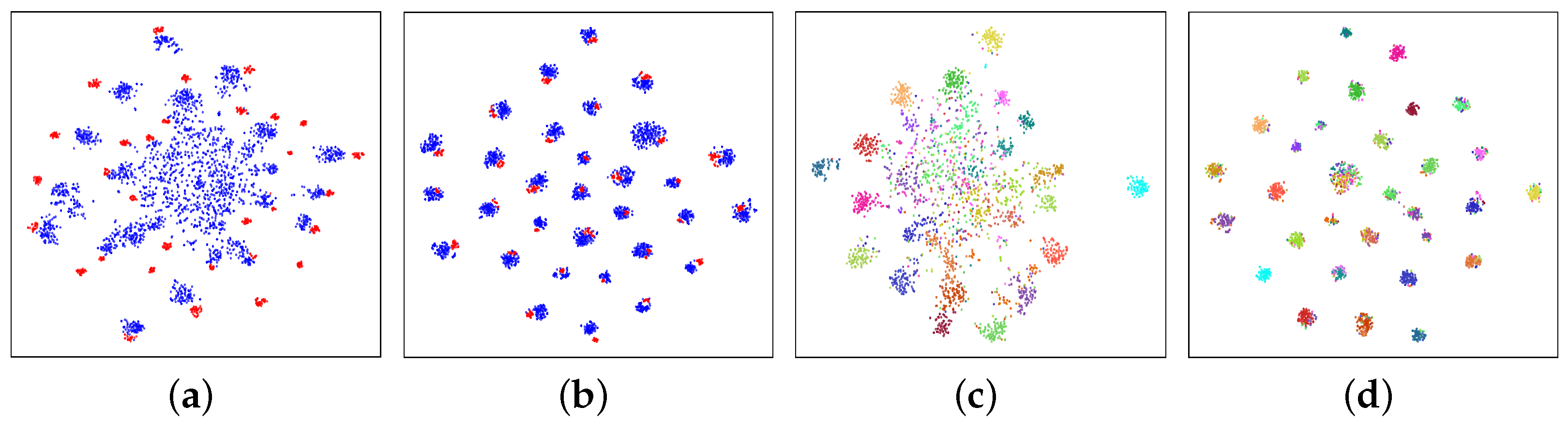
Feature visualization. For intuitively using the tool of t-SNE [78], we provide a feature analysis that visualizes the 31-way classification results of task W→A on Office-31. Figure 5a,b present the cluster distribution in the deep feature space defined by function $e_m\left(·;{\theta }_m\right)$, i.e., the feature extractor. Our method apparently leads to an implicit alignment from the target domain to the source domain. Figure 5c,d present distribution details. After model adaptation, the target data in the deep feature space satisfy a distribution with evident semantic meaning.

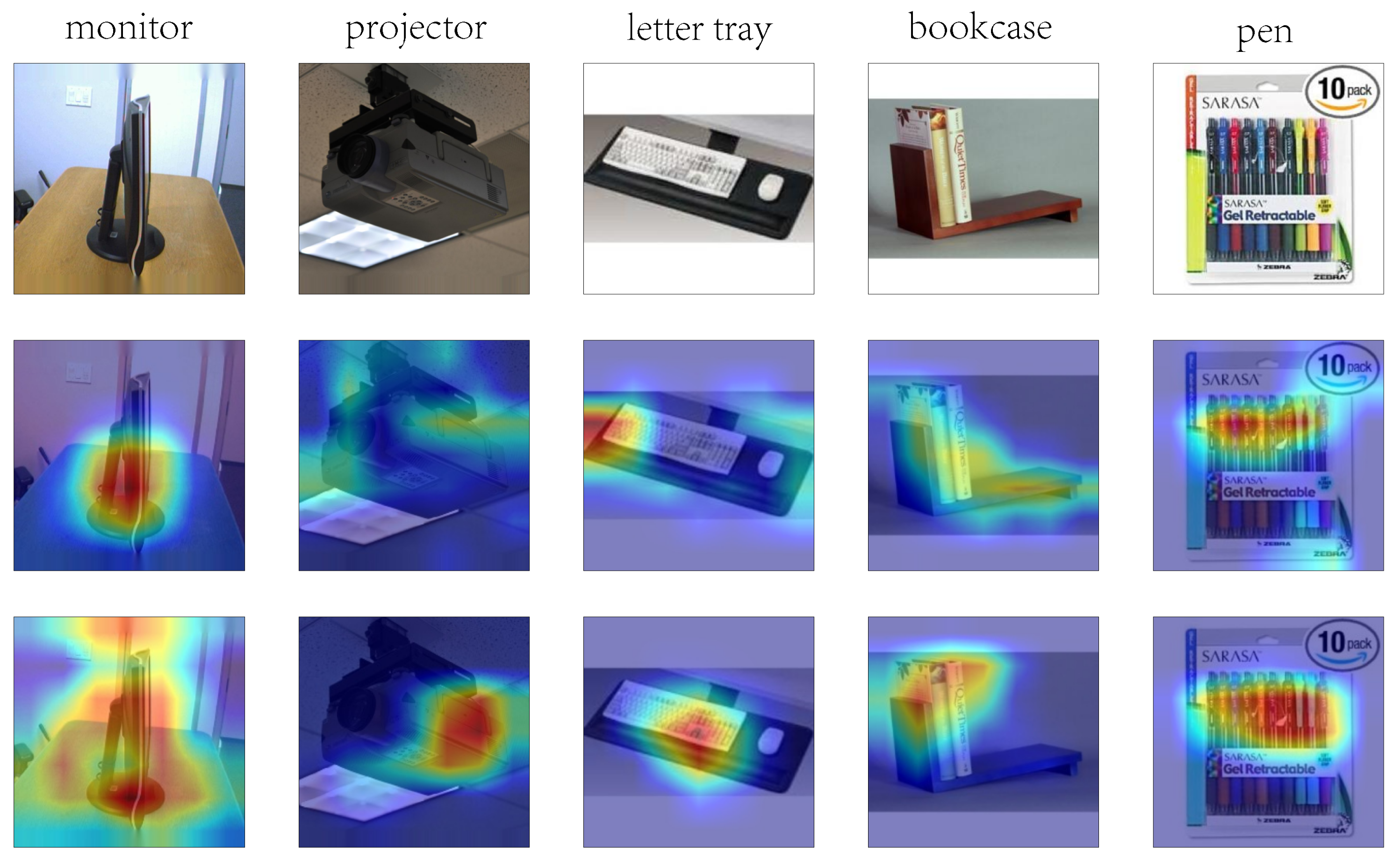
Grad-CAM visualization. To explain why our method works, we conduct a visualization analysis from the perspective of attention using the gradient-weighted class activation map (Grad-CAM) method [79]. As shown in the first row of Figure 6, we present some original images randomly selected from Office-31 and provide their Grad-CAM images from the source model and our method in the remaining two rows. As we are using the source model, we cannot clearly observe the attention phenomenon. For the projector, the active area representing attention is weak. For the bookcase, the red area representing strong attention covers the whole image. These attention patterns do not always lead to good results. In contrast, based on our method, attention occurs and focuses on the key components of these objects.

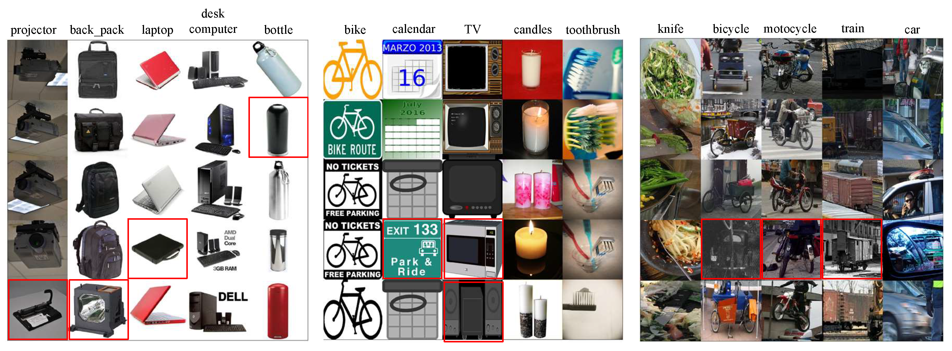
Geometry-guided knowledge visualization. For our method, the constructed geometry-guided knowledge plays a central role. To show the working mechanism of it, we visualize the proposed neighborhood modeling the knowledge in Figure 7. From the misclassified images on the three datasets for object recognition, we randomly choose 15 example images, as shown in the first row of Figure 7, and arrange the samples in their neighborhood in the other rows. It emerges that most of the neighborhood samples have the same categories as the corresponding original images. Thus, these neighborhood samples can provide comprehensive semantic information to correct the wrong classification on these original images.

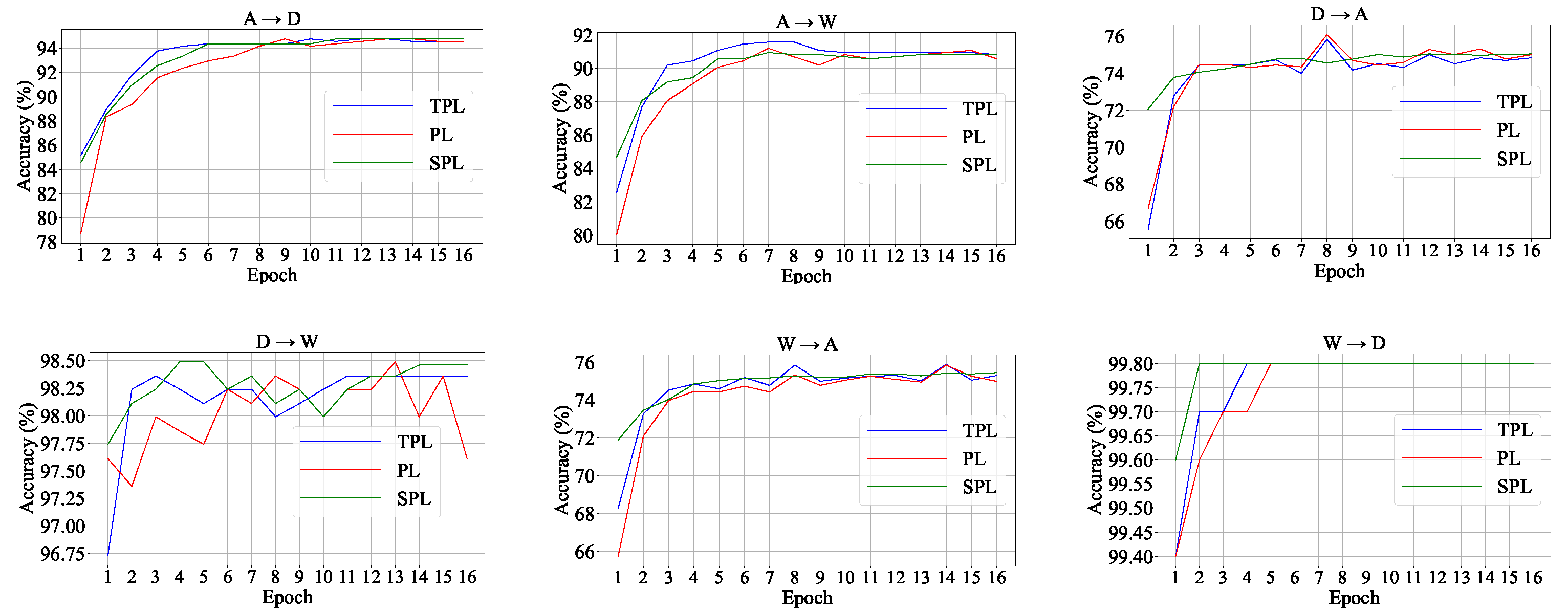
We implement the correction mentioned above by the semantic fusion formulated in Equation (3) and (6). Here, we plot the classification accuracies of soft pseudo-labels on Office-31 during the training phase in Figure 8. As a comparison, we also present the classification accuracies of pseudo-labels without the semantic fusion and the classification accuracy of pseudo-labels of the teacher model. For clarity, we denote the three methods as SPL, PL, and TPL, respectively. On all six adaptation tasks on Office-31, SPL consistently demonstrates superior performance compared to PL and TPL. This accuracy gap in Figure 8 also explains the performance decrease caused by canceling the soft pseudo-label that we discussed in the ablation study (see the fourth row and the last row in

Table 6. Results of ablation study for the effects of geometry-guided knowledge. Blue bold means best result.

Methods/Datasets	Office-31	Office-Home	VisDA
Source model only	78.5	59.4	51.2
G2KD with ${\mathcal{L}}_{\mathrm{ent}}+{\mathcal{L}}_{\mathrm{dis}}^{\mathrm{raw}}+{\mathcal{L}}_{\mathrm{stu}}^{\mathrm{raw}}$	88.9	71.5	82.1
G2KD with ${\mathcal{L}}_{\mathrm{ent}}+{\mathcal{L}}_{\mathrm{dis}}^{\mathrm{raw}}+{\mathcal{L}}_{\mathrm{stu}}$	89.6	71.9	83.0
G2KD with ${\mathcal{L}}_{\mathrm{ent}}+{\mathcal{L}}_{\mathrm{dis}}+{\mathcal{L}}_{\mathrm{stu}}^{\mathrm{raw}}$	89.2	72.3	84.4
G2KD with standard k-means	88.1	71.0	82.3
G2KD	90.0	72.5	85.4

).

Training resource demands. In order to more objectively evaluate the required training resources, we selected three representative SFDA methods, SHOT, AaD, and NRC, as comparison baselines. Experimental comparisons were conducted on the Ar → Cl migration task of the Office-Home dataset under the same test conditions, and the relevant results are shown in

Table 7. Comparison of training resource demands (per iter.) on Ar→Cl in Office-Home. Blue bold means best result.

#	Item/Method	SHOT [13]	AaD [80]	NRC [73]	G2KD
1	GPU memory consumption ↓ (G)	7.868	9.622	9.851	7.638
2	Training times ↓ (s)	0.407	0.547	0.491	0.484

. Despite the need to recalculate the neighborhood geometry and perform clustering and semantic fusion operations at each stage, the experimental results show that our method remains within a reasonable range in terms of memory usage and training time per epoch, and the computational overhead is controllable.

Sensitivity to hyper-parameters. In G2KD, D is the neighborhood size, and $\alpha$ in $L_e$ (Equation (7)) is the trade-off parameters. We test their sensitivity of performance on the symmetric transfer tasks Cl→Ar and Ar→Cl in Office-Home. Specifically, as shown in Figure 9, the performance achieves the best result as D takes an intermediate value. A smaller value leads to insufficient information, whilst a larger value introduces more noise. The results are consistent with our expectations. As for $\alpha$, it is seen that our method is highly robust to its settings.

4.6. Ablation Study

In this part, we isolate the effect of the critical components in G2KD. These components include (1) the gradual distillation strategy, (2) the geometry-guided knowledge, and (3) the regularization losses in our objective.

Effect of gradual distillation strategy. As noted, for G2KD, the teacher model ${\mathrm{IntM}}_{m-1}$ provides the supervision for the distillation, i.e., soft target ${\overline{\mathit{o}}}_i$ in ${\mathcal{L}}_{\mathrm{dis}}$ and soft pseudo-label ${\overline{\mathit{l}}}_i$ in ${\mathcal{L}}_{\mathrm{stu}}$. To verify the effect of the gradual distillation strategy, we cancel this strategy from the training process by imposing a replacement operation on the supervision. Specifically, for a supervision, ${\overline{\mathit{o}}}_i$ or ${\overline{\mathit{l}}}_i$, we generate it by the source model $f_s$, then fix it during the whole adaptation phase. In this way, we have three evaluation cases, as reported in

Table 8. Ablation study for the gradual distillation strategy on VisDA. $〈s〉$ denotes the supervision used in ${\mathcal{L}}_{\mathrm{dis}}$ and ${\mathcal{L}}_{\mathrm{stu}}$; i.e., soft target ${\overline{\mathit{o}}}_i$ and soft pseudo-label ${\overline{\mathit{l}}}_i$ are generated by the source model $f_s$. $〈t〉$ means the supervision is generated by the teacher model ${\mathrm{M}}_{m-1}$. Blue bold means best result.

${\mathcal{L}}_{\mathbf{ent}}$	${\mathcal{L}}_{\mathbf{dis}}$	${\mathcal{L}}_{\mathbf{stu}}$	Per-Class
✓	$〈s〉$	$〈s〉$	71.1
✓	$〈s〉$	$〈t〉$	81.5
✓	$〈t〉$	$〈s〉$	83.4
✓	$〈t〉$	$〈t〉$	85.4

.

As shown in the first row in Table 8, when both ${\overline{\mathit{o}}}_i$ and ${\overline{\mathit{l}}}_i$ are replaced, there is large gap of 14.3% compared to the full version shown in the fourth row. As shown in the following two rows, when ${\overline{\mathit{o}}}_i$ or ${\overline{\mathit{l}}}_i$ is replaced, the average accuracy has evident improvement (increase by 10.4% at least). The comparison indicates that the gradual distillation strategy has a great influence on the final result. This progressive process can well capture the dynamics of data geometric structure during the transfer phase.

Effects of geometry-guided knowledge. G2KD takes the soft target and the soft pseudo-label, based on geometry-guided knowledge, to regulate the distillation loss ${\mathcal{L}}_{\mathrm{dis}}$ and the student loss ${\mathcal{L}}_{\mathrm{stu}}$, respectively. To present the advantages of introducing geometry-guided knowledge, we use the raw information without the semantic fusion as the supervision. Correspondingly, we rewrite the two knowledge distillation losses as the following raw form.

$$\begin{array}{cc}\hfill {\mathcal{L}}_{\mathrm{dis}}^{\mathrm{raw}}& =\mathrm{KL}\left({\overline{\mathit{p}}}_i\left|\right|{\mathit{p}}_i^{\prime }\right),\hfill \\ \hfill {\mathcal{L}}_{\mathrm{stu}}^{\mathrm{raw}}& =-\beta {\displaystyle \frac{1}{n}}\sum _{i=1}^{n_t}\sum _{k=1}^K{\mathbf{l}}_{i,k}^{t}log{\phi }_k\left({\tilde{\mathit{x}}}_{im}^t\right)+\gamma \sum _{k=1}^K{\varrho }_{k}log{\varrho }_k.\hfill \end{array}$$

(13)

where ${\overline{\mathit{p}}}_i$ and ${\mathbf{l}}_{i,k}^t=\mathrm{I}\left[k={\overline{y}}_i\right]$ are the raw target and the raw pseudo-label, respectively, and the other notations are the same as the ones in Equations (9) and (10). Here, we present three primary cases to evaluate the geometry-guided knowledge effect. The first is G2KD without the soft target where we replace ${\mathcal{L}}_{\mathrm{dis}}$ with ${\mathcal{L}}_{\mathrm{dis}}^{\mathrm{raw}}$, while the second is G2KD without the soft pseudo-label where we replace ${\mathcal{L}}_{\mathrm{stu}}$ with ${\mathcal{L}}_{\mathrm{stu}}^{\mathrm{raw}}$. The third is G2KD without both soft target and soft pseudo-label. Also, we evaluate the three component losses in our objective ${\mathcal{L}}_{\mathrm{G}2\mathrm{KD}}$, i.e., ${\mathcal{L}}_{\mathrm{ent}}$, ${\mathcal{L}}_{\mathrm{dis}}$, and ${\mathcal{L}}_{\mathrm{stu}}$.

Table 6 reports the ablation study results. Comparing the results in the last row with the results from the second row to fourth row, we observe that geometry-guided knowledge can lead to evident improvement on the three datasets. G2KD with geometry-guided knowledge beats the three G2KD variations without geometry-guided knowledge. This comparison indicates the importance of the geometry-guided knowledge distillation that this paper develops. In the fifth row, G2KD with standard k-means refers to applying standard k-means clustering without the weighting mechanism described in Equation (4). It is seen that standard k-means leads to noticeable drops on all three datasets, confirming the effect of our weighting strategy.

Effects of regularization losses. We adopt an incremental way to evaluate these losses. We take the variation method trained by only ${\mathcal{L}}_{\mathrm{ent}}$ as baseline and then add losses ${\mathcal{L}}_{\mathrm{dis}}$ and ${\mathcal{L}}_{\mathrm{stu}}$ one by one. As shown in

Table 9. Results of ablation study for the effects of regularization losses. Blue bold means best result.

${\mathcal{L}}_{\mathbf{ent}}$	${\mathcal{L}}_{\mathbf{dis}}$	${\mathcal{L}}_{\mathbf{stu}}$	Office-31	Office-Home	VisDA
✓	✗	✗	83.9	61.1	80.5
✓	✓	✗	85.7	68.9	81.6
✓	✗	✓	88.3	71.1	84.3
✓	✓	✓	90.0	72.5	85.4

, the objective combining ${\mathcal{L}}_{\mathrm{ent}}$ with ${\mathcal{L}}_{\mathrm{dis}}$ or ${\mathcal{L}}_{\mathrm{stu}}$ obtains much better results than merely using ${\mathcal{L}}_{\mathrm{ent}}$ as the objective. We achieve the best results on the three datasets when ${\mathcal{L}}_{\mathrm{ent}}$, ${\mathcal{L}}_{\mathrm{dis}}$, and ${\mathcal{L}}_{\mathrm{stu}}$ work simultaneously. These ablation results show that our losses positively affect the final performance.

5. Conclusions

This paper proposes a new self-supervised learning method, G2KD, which solves SFDA by Gradual Geometry-Guided Knowledge Distillation. This method offers a different perspective for the challenging SFDA problem. Specifically, to bypass the absence of the source data, we perform self-learning on the target domain via mix-entropy minimization, which absorbs neighbor context. At the same time, we perform geometry-guided knowledge distillation, in which we construct a neighborhood geometry to model the knowledge and use it to guide the distillation. Experiments on four challenging benchmarks indicate that our method achieves state-of-the-art performance.

References

1. Hoffman, J.; Tzeng, E.; Park, T.; Zhu, J.; Isola, P.; Saenko, K.; Efros, A.; Darrell, T. CyCADA: Cycle-Consistent Adversarial Domain Adaptation. In Proceedings of the 35th International Conference on Machine Learning (ICML), Stockholm, Sweden, 10–15 July 2018; pp. 1989–1998. [Google Scholar]
2. Long, M.; Cao, Z.; Wang, J.; Jordan, M. Conditional Adversarial Domain Adaptation. In Proceedings of the 32nd International Conference on Neural Information Processing Systems (NeurIPS), Montréal, QC, Canada, 2–8 December 2018; pp. 1647–1657. [Google Scholar]
3. Ronneberger, O.; Fischer, P.; Brox, T. U-Net: Convolutional Networks for Biomedical Image Segmentation. In Proceedings of the International Conference on Medical Image Computing and Computer-Assisted Intervention (MICCAI), Munich, Germany, 5–9 October 2015; pp. 234–241. [Google Scholar]
4. Milletari, F.; Navab, N.; Ahmadi, S.A. V-Net: Fully Convolutional Neural Networks for Volumetric Medical Image Segmentation. In Proceedings of the 4th International Conference on 3D Vision (3DV), Stanford, CA, USA, 25–28 October 2016; pp. 565–571. [Google Scholar]
5. Chidlovskii, B.; Clinchant, S.; Csurka, G. Domain Adaptation in the Absence of Source Domain Data. In Proceedings of the 22nd ACM SIGKDD International Conference on Knowledge Discovery and Data Mining (KDD), San Francisco, CA, USA, 13–17 August 2016; pp. 451–460. [Google Scholar]
6. Liang, J.; He, R.; Sun, Z.; Tan, T. Distant Supervised Centroid Shift: A Simple and Efficient Approach to Visual Domain Adaptation. In Proceedings of the IEEE/CVF Conference on Computer Vision and Pattern Recognition (CVPR), Long Beach, CA, USA, 16–20 June 2019; pp. 2975–2984. [Google Scholar]
7. Lao, Q.; Jiang, X.; Havaei, M. Hypothesis Disparity Regularized Mutual Information Maximization. In Proceedings of the AAAI Conference on Artificial Intelligence (AAAI), Virtual, 2–9 February 2021; pp. 8243–8251. [Google Scholar]
8. Qiu, Z.; Zhang, Y.; Lin, H.; Niu, S.; Liu, Y.; Du, Q.; Tan, M. Source-free domain adaptation via avatar prototype generation and adaptation. In Proceedings of the 30th International Joint Conference on Artificial Intelligence (IJCAI), Montreal, QC, Canada, 19–27 August 2021; pp. 2921–2927. [Google Scholar]
9. Li, R.; Jiao, Q.; Cao, W.; Wong, H.S.; Wu, S. Model Adaptation: Unsupervised Domain Adaptation Without Source Data. In Proceedings of the IEEE/CVF Conference on Computer Vision and Pattern Recognition (CVPR), Virtual, 14–19 June 2020; pp. 9638–9647. [Google Scholar]
10. Kim, Y.; Cho, D.; Han, K.; Panda, P.; Hong, S. Domain Adaptation Without Source Data. IEEE Trans. Artif. Intell. 2021, 2, 508–518. [Google Scholar] [CrossRef]
11. Tian, J.; Zhang, J.; Li, W.; Xu, D. VDM-DA: Virtual domain modeling for source data-free domain adaptation. IEEE Trans. Circuits Syst. Video Technol. 2022, 32, 3749–3760. [Google Scholar] [CrossRef]
12. Li, J.; Du, Z.; Zhu, L.; Ding, Z.; Lu, K.; Shen, H.T. Divergence-Agnostic Unsupervised Domain Adaptation by Adversarial Attacks. IEEE Trans. Pattern Anal. Mach. Intell. 2022, 44, 8196–8211. [Google Scholar] [CrossRef] [PubMed]
13. Liang, J.; Hu, D.; Feng, J. Do We Really Need to Access the Source Data? Source Hypothesis Transfer for Unsupervised Domain Adaptation. In Proceedings of the 37th International Conference on Machine Learning (ICML), Virtual, 13–18 July 2020; pp. 6028–6039. [Google Scholar]
14. Li, S.; Xie, M.; Gong, K.; Liu, C.H.; Wang, Y.; Li, W. Transferable Semantic Augmentation for Domain Adaptation. In Proceedings of the IEEE Conference on Computer Vision and Pattern Recognition (CVPR), Virtual, 19–25 June 2021; pp. 11516–11525. [Google Scholar]
15. Yang, S.; Wang, Y.; van de Weijer, J.; Herranz, L.; Jui, S. Unsupervised domain adaptation without source data by casting a bait. arXiv 2020, arXiv:2010.12427. [Google Scholar]
16. Yu, Y.; Min, X.; Zhao, S.; Mei, J.; Wang, F.; Li, D.; Ng, K.; Li, S. Dynamic Knowledge Distillation for Black-box Hypothesis Transfer Learning. arXiv 2020, arXiv:2007.12355. [Google Scholar]
17. Zhang, B.; Zhang, X.; Liu, Y.; Cheng, L.; Li, Z. Matching Distributions between Model and Data: Cross-domain Knowledge Distillation for Unsupervised Domain Adaptation. In Proceedings of the 59th Annual Meeting of the Association for Computational Linguistics and the 11th International Joint Conference on Natural Language Processing (ACL-IJCNLP), Bangkok, Thailand, 1–6 August 2021; pp. 5423–5433. [Google Scholar]
18. Yang, G.; Tang, H.; Zhong, Z.; Ding, M.; Shao, L.; Sebe, N.; Ricci, E. Transformer-Based Source-Free Domain Adaptation. arXiv 2021, arXiv:2105.14138. [Google Scholar]
19. Furlanello, T.; Lipton, Z.; Tschannen, M.; Itti, L.; Anandkumar, A. Born Again Neural Networks. In Proceedings of the 35th International Conference on Machine Learning (ICML), Stockholm, Sweden, 10–15 July 2018; pp. 1607–1616. [Google Scholar]
20. Yuan, L.; Tay, F.E.; Li, G.; Wang, T.; Feng, J. Revisiting Knowledge Distillation via Label Smoothing Regularization. In Proceedings of the IEEE/CVF Conference on Computer Vision and Pattern Recognition (CVPR), Virtual, 14–19 June 2020; pp. 3903–3911. [Google Scholar]
21. Long, M.; Cao, Y.; Wang, J.; Jordan, M. Learning Transferable Features with Deep Adaptation Networks. In Proceedings of the 32nd International Conference on Machine Learning (ICML), Lille, France, 6–11 July 2015; pp. 97–105. [Google Scholar]
22. Pan, Y.; Yao, T.; Li, Y.; Wang, Y.; Ngo, C.W.; Mei, T. Transferrable Prototypical Networks for Unsupervised Domain Adaptation. In Proceedings of the IEEE/CVF Conference on Computer Vision and Pattern Recognition (CVPR), Long Beach, CA, USA, 16–20 June 2019; pp. 2239–2247. [Google Scholar]
23. Tzeng, E.; Hoffman, J.; Zhang, N.; Saenko, K.; Darrell, T. Deep domain confusion: Maximizing for domain invariance. arXiv 2014, arXiv:1412.3474. [Google Scholar]
24. Zhang, Y.; Tang, H.; Jia, K.; Tan, M. Domain-Symmetric Networks for Adversarial Domain Adaptation. In Proceedings of the IEEE/CVF Conference on Computer Vision and Pattern Recognition (CVPR), Long Beach, CA, USA, 16–20 June 2019; pp. 5031–5040. [Google Scholar]
25. Munro, J.; Damen, D. Multi-Modal Domain Adaptation for Fine-Grained Action Recognition. In Proceedings of the IEEE/CVF Conference on Computer Vision and Pattern Recognition (CVPR), Virtual, 14–19 June 2020; pp. 119–129. [Google Scholar]
26. Gopalan, R.; Li, R.; Chellappa, R. Domain Adaptation for Object Recognition: An Unsupervised Approach. In Proceedings of the IEEE International Conference on Computer Vision (ICCV), Barcelona, Spain, 6–13 November 2011; pp. 999–1006. [Google Scholar]
27. Gong, B.; Shi, Y.; Sha, F.; Grauman, K. Geodesic Flow Kernel for Unsupervised Domain Adaptation. In Proceedings of the IEEE Conference on Computer Vision and Pattern Recognition (CVPR), Providence, RI, USA, 16–21 June 2012; pp. 2066–2073. [Google Scholar]
28. Caseiro, R.; Henriques, J.F.; Martins, P.; Batista, J. Beyond the shortest path: Unsupervised domain adaptation by sampling subspaces along the spline flow. In Proceedings of the IEEE Conference on Computer Vision and Pattern Recognition (CVPR), Boston, MA, USA, 7–12 June 2015; pp. 3846–3854. [Google Scholar]
29. Tang, S.; Ji, Y.; Lyu, J.; Mi, J.; Li, Q.; Zhang, J. Visual Domain Adaptation Exploiting Confidence-Samples. In Proceedings of the IEEE/RSJ International Conference on Intelligent Robots and Systems (IROS), Macau, China, 4–8 November 2019; pp. 1173–1179. [Google Scholar]
30. Pan, Y.; Yao, T.; Li, Y.; Ngo, C.W.; Mei, T. Exploring Category-Agnostic Clusters for Open-Set Domain Adaptation. In Proceedings of the IEEE/CVF Conference on Computer Vision and Pattern Recognition (CVPR), Virtual, 14–19 June 2020; pp. 13864–13872. [Google Scholar]
31. Zhang, Y.; Deng, B.; Jia, K.; Zhang, L. Label Propagation with Augmented Anchors: A Simple Semi-Supervised Learning Baseline for Unsupervised Domain Adaptation. In Proceedings of the 16th European Conference on Computer Vision (ECCV), Virtual, 23–28 August 2020; pp. 781–797. [Google Scholar]
32. Chen, Y.; Wang, Y.; Pan, Y.; Yao, T.; Tian, X.; Mei, T. A Style and Semantic Memory Mechanism for Domain Generalization. In Proceedings of the IEEE/CVF International Conference on Computer Vision (ICCV), Virtual, 11–17 October 2021; pp. 9164–9173. [Google Scholar]
33. Tang, S.; Ye, M.; Xu, P.; Li, X. Adaptive pedestrian detection by predicting classifier. Neural Comput. Appl. 2019, 31, 1189–1200. [Google Scholar] [CrossRef]
34. Tanwisuth, K.; Fan, X.; Zheng, H.; Zhang, S.; Zhang, H.; Chen, B.; Zhou, M. A Prototype-Oriented Framework for Unsupervised Domain Adaptation. In Proceedings of the 35th Conference on Neural Information Processing Systems (NeurIPS), Virtual, 6–14 December 2021; pp. 17194–17208. [Google Scholar]
35. Du, Y.; Yang, H.; Chen, M.; Jiang, J.; Luo, H.; Wang, C. Generation, augmentation, and alignment: A pseudo-source domain based method for source-free domain adaptation. arXiv 2021, arXiv:2109.04015. [Google Scholar] [CrossRef]
36. Hinton, G.; Vinyals, O.; Dean, J. Distilling the knowledge in a neural network. arXiv 2015, arXiv:1503.02531. [Google Scholar]
37. Romero, A.; Ballas, N.; Ebrahimi Kahou, S.; Chassang, A.; Gatta, C.; Bengio, Y. FitNets: Hints for Thin Deep Nets. In Proceedings of the 3rd International Conference on Learning Representations (ICLR), San Diego, CA, USA, 7–9 May 2015. [Google Scholar]
38. Passalis, N.; Tefas, A. Learning Deep Representations with Probabilistic Knowledge Transfer. In Proceedings of the 15th European Conference on Computer Vision (ECCV), Munich, Germany, 8–14 September 2018; pp. 283–299. [Google Scholar]
39. Zhang, L.; Song, J.; Gao, A.; Chen, J.; Bao, C.; Ma, K. Be Your Own Teacher: Improve the Performance of Convolutional Neural Networks via Self Distillation. In Proceedings of the IEEE/CVF International Conference on Computer Vision (ICCV), Seoul, Republic of Korea, 27 October–2 November 2019; pp. 3713–3722. [Google Scholar]
40. Yun, S.; Park, J.; Lee, K.; Shin, J. Regularizing Class-Wise Predictions via Self-Knowledge Distillation. In Proceedings of the IEEE/CVF Conference on Computer Vision and Pattern Recognition (CVPR), Virtual, 14–19 June 2020; pp. 13876–13885. [Google Scholar]
41. Yang, C.; Xie, L.; Su, C.; Yuille, A.L. Snapshot Distillation: Teacher-Student Optimization in One Generation. In Proceedings of the IEEE/CVF Conference on Computer Vision and Pattern Recognition (CVPR), Long Beach, CA, USA, 15–20 June 2019; pp. 2859–2868. [Google Scholar]
42. Kim, K.; Ji, B.; Yoon, D.; Hwang, S. Self-knowledge distillation with progressive refinement of targets. arXiv 2020, arXiv:2006.12000. [Google Scholar]
43. Zhang, H.; Zhang, Y.; Jia, K.; Zhang, L. Unsupervised Domain Adaptation of Black-Box Source Models. In Proceedings of the 32nd British Machine Vision Conference (BMVC), Virtual, 22–25 November 2021; pp. 8003–8013. [Google Scholar]
44. Liang, J.; Hu, D.; Feng, J.; He, R. DINE: Domain Adaptation from Single and Multiple Black-box Predictors. In Proceedings of the IEEE/CVF Conference on Computer Vision and Pattern Recognition (CVPR), New Orleans, LA, USA, 19–24 June 2022; pp. 8003–8013. [Google Scholar]
45. Ghasedi Dizaji, K.; Herandi, A.; Deng, C.; Cai, W.; Huang, H. Deep Clustering via Joint Convolutional Autoencoder Embedding and Relative Entropy Minimization. In Proceedings of the IEEE International Conference on Computer Vision (ICCV), Venice, Italy, 22–29 October 2017; pp. 5736–5745. [Google Scholar]
46. Melacci, S.; Gori, M. Unsupervised learning by minimal entropy encoding. IEEE Trans. Neural Netw. Learn. Syst. 2012, 23, 1849–1861. [Google Scholar] [CrossRef] [PubMed]
47. Niu, G.; Dai, B.; Yamada, M.; Sugiyama, M. Information-theoretic semi-supervised metric learning via entropy regularization. Neural Comput. 2014, 26, 1717–1762. [Google Scholar] [CrossRef] [PubMed]
48. Ji, X.; Henriques, J.F.; Vedaldi, A. Invariant information clustering for unsupervised image classification and segmentation. In Proceedings of the IEEE/CVF International Conference on Computer Vision (ICCV), Seoul, Republic of Korea, 27 October–2 November 2019; pp. 9865–9874. [Google Scholar]
49. Paninski, L. Estimation of entropy and mutual information. Neural Comput. 2003, 15, 1191–1253. [Google Scholar] [CrossRef]
50. Tang, H.; Chen, K.; Jia, K. Unsupervised Domain Adaptation via Structurally Regularized Deep Clustering. In Proceedings of the IEEE Conference on Computer Vision and Pattern Recognition (CVPR), Virtual, 14–19 June 2020; pp. 8722–8732. [Google Scholar]
51. Krause, A.; Perona, P.; Gomes, R. Discriminative Clustering by Regularized Information Maximization. In Proceedings of the Advances in Neural Information Processing Systems (NeurIPS), Vancouver, BC, Canada, 6–9 December 2010; pp. 775–783. [Google Scholar]
52. Saenko, K.; Kulis, B.; Fritz, M.; Darrell, T. Adapting visual category models to new domains. In Proceedings of the European Conference on Computer Vision (ECCV), Heraklion, Greece, 5–11 September 2010; pp. 213–226. [Google Scholar]
53. Venkateswara, H.; Eusebio, J.; Chakraborty, S.; Panchanathan, S. Deep hashing network for unsupervised domain adaptation. In Proceedings of the IEEE Conference on Computer Vision and Pattern Recognition (CVPR), Honolulu, HI, USA, 21–26 July 2017; pp. 5385–5394. [Google Scholar]
54. Peng, X.; Usman, B.; Kaushik, N.; Hoffman, J.; Wang, D.; Saenko, K. Visda: The visual domain adaptation challenge. arXiv 2017, arXiv:1710.06924. [Google Scholar]
55. Peng, X.; Bai, Q.; Xia, X.; Huang, Z.; Saenko, K.; Wang, B. Moment matching for multi-source domain adaptation. In Proceedings of the IEEE International Conference on Computer Vision (ICCV), Seoul, Republic of Korea, 27 October–2 November 2019; pp. 1406–1415. [Google Scholar]
56. Xu, R.; Li, G.; Yang, J.; Lin, L. Larger norm more transferable: An adaptive feature norm approach for unsupervised domain adaptation. In Proceedings of the IEEE International Conference on Computer Vision (ICCV), Virtual, 29 October–2 November 2019; pp. 1426–1435. [Google Scholar]
57. He, K.; Zhang, X.; Ren, S.; Sun, J. Deep residual learning for image recognition. In Proceedings of the IEEE Conference on Computer Vision and Pattern Recognition (CVPR), Las Vegas, NV, USA, 27 June–2 July 2016; pp. 1180–1189. [Google Scholar]
58. Lee, C.Y.; Batra, T.; Baig, M.H.; Ulbricht, D. Sliced wasserstein discrepancy for unsupervised domain adaptation. In Proceedings of the IEEE Conference on Computer Vision and Pattern Recognition (CVPR), Long Beach, CA, USA, 15–20 July 2019; pp. 10285–10295. [Google Scholar]
59. Wu, Y.; Inkpen, D.; El-Roby, A. Dual mixup regularized learning for adversarial domain adaptation. In Proceedings of the European Conference on Computer Vision (ECCV), Virtual, 23–28 August 2020; pp. 540–555. [Google Scholar]
60. Chen, X.; Wang, S.; Long, M.; Wang, J. Transferability vs. discriminability: Batch spectral penalization for adversarial domain adaptation. In Proceedings of the International Conference on Machine Learning (ICML), Long Beach, CA, USA, 9–15 June 2019; pp. 1081–1090. [Google Scholar]
61. Wang, X.; Jin, Y.; Long, M.; Wang, J.; Jordan, M. Transferable normalization: Towards improving transferability of deep neural networks. In Proceedings of the Advances in Neural Information Processing Systems (NeurIPS), Vancouver, BC, Canada, 8–14 December 2019; pp. 1951–1961. [Google Scholar]
62. Jiang, X.; Lao, Q.; Matwin, S.; Havaei, M. Implicit Class-Conditioned Domain Alignment for Unsupervised Domain Adaptation. In Proceedings of the International Conference on Machine Learning (ICML), Virtual, 12–18 July 2020; Volume 119, pp. 4816–4827. [Google Scholar]
63. Cui, S.; Wang, S.; Zhuo, J.; Li, L.; Huang, Q.; Tian, Q. Towards discriminability and diversity: Batch nuclear-norm maximization under label insufficient situations. In Proceedings of the IEEE Conference on Computer Vision and Pattern Recognition (CVPR), Virtual, 14–19 June 2020; pp. 3940–3949. [Google Scholar]
64. Jin, Y.; Wang, X.; Long, M.; Wang, J. Minimum Class Confusion for Versatile Domain Adaptation. In Proceedings of the European Conference on Computer Vision (ECCV), Virtual, 23–28 August 2020; pp. 464–480. [Google Scholar]
65. Du, Z.; Li, J.; Su, H.; Zhu, L.; Lu, K. Cross-domain gradient discrepancy minimization for unsupervised domain adaptation. In Proceedings of the IEEE Conference on Computer Vision and Pattern Recognition (CVPR), Virtual, 19–25 June 2021; pp. 3937–3946. [Google Scholar]
66. Huang, J.; Guan, D.; Xiao, A.; Lu, S.; Shao, L. Category contrast for unsupervised domain adaptation in visual tasks. In Proceedings of the IEEE Conference on Computer Vision and Pattern Recognition (CVPR), New Orleans, LA, USA, 19–24 June 2022; pp. 1203–1214. [Google Scholar]
67. Zhang, J.; Huang, J.; Tian, Z.; Lu, S. Spectral unsupervised domain adaptation for visual recognition. In Proceedings of the IEEE Conference on Computer Vision and Pattern Recognition (CVPR), New Orleans, LA, USA, 19–24 June 2022; pp. 9829–9840. [Google Scholar]
68. Venkat, N.; Kundu, J.N.; Singh, D.; Revanur, A.; Babu, R.V. Your classifier can secretly suffice multi-source domain adaptation. In Proceedings of the Advances in Neural Information Processing Systems (NeurIPS), Virtual, 6–12 December 2020; Volume 33, pp. 4647–4659. [Google Scholar]
69. Scalbert, M.; Vakalopoulou, M.; Couzinié-Devy, F. Multi-source domain adaptation via supervised contrastive learning and confident consistency regularization. In Proceedings of the British Machine Vision Conference (BMVC), Virtual, 22–25 November 2021. Paper 0699. [Google Scholar]
70. Li, Y.; Yuan, L.; Chen, Y.; Wang, P.; Vasconcelos, N. Dynamic transfer for multi-source domain adaptation. In Proceedings of the IEEE Conference on Computer Vision and Pattern Recognition (CVPR), Virtual, 19–25 June 2021; pp. 10998–11007. [Google Scholar]
71. Nguyen, V.A.; Nguyen, T.; Le, T.; Tran, Q.H.; Phung, D. Stem: An approach to multi-source domain adaptation with guarantees. In Proceedings of the IEEE Conference on Computer Vision and Pattern Recognition (CVPR), Virtual, 19–25 June 2021; pp. 9352–9363. [Google Scholar]
72. Ahmed, S.M.; Raychaudhuri, D.S.; Paul, S.; Oymak, S.; Roy-Chowdhury, A.K. Unsupervised multi-source domain adaptation without access to source data. In Proceedings of the IEEE Conference on Computer Vision and Pattern Recognition (CVPR), Virtual, 19–25 June 2021; pp. 10103–10112. [Google Scholar]
73. Yang, S.; Van de Weijer, J.; Herranz, L.; Jui, S. Exploiting the intrinsic neighborhood structure for source-free domain adaptation. In Proceedings of the Advances in Neural Information Processing Systems (NeurIPS), Virtual, 6–12 December 2021; Volume 34, pp. 29393–29405. [Google Scholar]
74. Tang, S.; Shi, Y.; Ma, Z.; Li, J.; Lyu, J.; Li, Q.; Zhang, J. Model adaptation through hypothesis transfer with gradual knowledge distillation. In Proceedings of the IEEE/RSJ International Conference on Intelligent Robots and Systems (IROS), Prague, Czech Republic, 27 September–1 October 2021; pp. 10103–10112. [Google Scholar]
75. Berthelot, D.; Carlini, N.; Goodfellow, I.; Papernot, N.; Oliver, A.; Raffel, C.A. Mixmatch: A holistic approach to semi-supervised learning. In Proceedings of the Advances in Neural Information Processing Systems (NeurIPS), Vancouver, BC, Canada, 8–14 December 2019; pp. 5049–5059. [Google Scholar]
76. Dosovitskiy, A.; Beyer, L.; Kolesnikov, A.; Weissenborn, D.; Zhai, X.; Unterthiner, T.; Dehghani, M.; Minderer, M.; Heigold, G.; Gelly, S.; et al. An image is worth 16 × 16 words: Transformers for image recognition at scale. arXiv 2020, arXiv:2010.11929. [Google Scholar]
77. Liang, J.; Hu, D.; Wang, Y.; He, R.; Feng, J. Source data-absent unsupervised domain adaptation through hypothesis transfer and labeling transfer. IEEE Trans. Pattern Anal. Mach. Intell. 2021, 44, 8602–8617. [Google Scholar] [CrossRef] [PubMed]
78. Van der Maaten, L.; Hinton, G. Visualizing data using t-SNE. J. Mach. Learn. Res. 2008, 9, 2579–2605. [Google Scholar]
79. Gildenblat, J.; Contributors. PyTorch Library for CAM Methods. 2021. Available online: https://github.com/jacobgil/pytorch-grad-cam (accessed on 20 April 2025).
80. Yang, S.; Wang, Y.; Wang, K.; Jui, S.; van de Weijer, J. Attracting and dispersing: A simple approach for source-free domain adaptation. Adv. Neural Inf. Process. Syst. 2022, 35, 5802–5815. [Google Scholar]
Figure 1. Comparing different knowledge-distillation-based SFDA frameworks. (a) Using a fixed source model as the teacher with the limitation that the semantic guidance will gradually weaken (i.e., guidance degradation) [16,17]. (b) Using a dynamical tracking model as the teacher [18]. The semantic noise would progressively amplify by the parameter updating strategy for tracking, hampering the distillation effect. (c) Our G2KD overcoming both limitations: At the global level, it trains N intermediate models to snapshot the semantics variation for guidance degradation mitigation in an epoch-wise manner. Second, at the local level, we adopt a self-distillation strategy (using the previous epoch model as the teacher) for providing more credible guidance.
Mathematics 13 01491 g001
Figure 2. An overview of sub-transfer driven by G2KD. At the beginning of a specific epoch, the student model M m is initialized by the pre-trained teacher model M m 1 . After that, given an input instance x i , (a) the geometry-guided knowledge module mines the knowledge by discovering local geometry over the target dataset for x i and then represents it to a corresponding soft supervision pair, as illustrated in (c), including soft target o ¯ i (Equation (3)) and soft pseudo-label l ¯ i (Equation (6)). During training, x i is feed-forwarded into the student model M m to obtain the soft output p ^ i and prediction pi. Combining with the presented geometry-guided knowledge (the soft supervision pair), (b) we perform the geometry-guided knowledge distillation. This is driven by the G2KD regularization (Equation (12)), consisting of an entropy loss L ent , a distillation loss L dis , and a student loss L stu .
Mathematics 13 01491 g002
Figure 3. Illustration of knowledge mining. (a) The neighborhood geometry of a specific target sample ( z i ) is taken as the knowledge. (b) By a simple semantic fusion on this local structure, a target sample of TV wrongly predicted as Oven can be corrected.
Mathematics 13 01491 g003
Figure 4. Confusion matrices for 31-way classification tasks W→A and A→W on the Office-31 dataset. Specifically, (a,b) present the results of the source model and G2KD in task A→W; (c,d) present the results of the source model and G2KD in task W→A, respectively.
Mathematics 13 01491 g004
Figure 5. Feature visualizations for task W→A on the Office-31 dataset. (a,b) Feature alignments by the source model and G2KD, respectively; (c,d) are semantic clustering by the source model and G2KD. In (a,b), red circles denote the features of the absent source data, and blue circles denote the features of the target data. In (c,d), for better category illustration, all 31 categories in each domain are selected, and a different color denotes a different category.
Mathematics 13 01491 g005
Figure 6. Typical Grad-CAM visualization on the Office-31 dataset. The first row presents the original example images. The second and third rows present the results of the source model only and of our method, respectively.
Mathematics 13 01491 g006
Figure 7. Visualization of neighborhood representing the geometry-guided knowledge on the three datasets for object recognition task. The left, middle, and right parts are randomly selected from Office-31, Office-Home, and VisDA, respectively. The first row presents the misclassified example images. The other rows show the samples in the neighborhood modeling the knowledge (the red squares mark the samples whose categories are different from the original images, i.e., the failure cases). The distance to the original images of these samples from the second row to the fifth row gradually increases.
Mathematics 13 01491 g007
Figure 8. The accuracy comparison of SPLs (soft pseudo-labels), PLs (pseudo-labels), and TPLs (teacher pseudo-labels) during model adaptation on the Office-31 dataset. The blue, red, and green curves stand for the accuracies of SPLs, PLs, and TPLs, respectively.
Mathematics 13 01491 g008
Figure 9. Sensitivity of hyper-parameters D and α , respectively.
Mathematics 13 01491 g009