Abstract
A Bayesian network offers powerful knowledge representations for independence, conditional independence and causal relationships among variables in a given domain. Despite its wide application, the detection limits of modern measurement technologies make the use of the Bayesian networks theoretically unfounded, even when the assumption of a multivariate Gaussian distribution is satisfied. In this paper, we introduce the censored Gaussian Bayesian network (GBN), an extension of GBNs designed to handle left- and right-censored data caused by instrumental detection limits. We further propose the censored Structural Expectation-Maximization (cSEM) algorithm, an iterative score-and-search framework that integrates Monte Carlo sampling in the E-step for efficient expectation computation and employs the iterative Markov chain Monte Carlo (MCMC) algorithm in the M-step to refine the network structure and parameters. This approach addresses the non-decomposability challenge of censored-data likelihoods. Through simulation studies, we illustrate the superior performance of the cSEM algorithm compared to the existing competitors in terms of network recovery when censored data exist. Finally, the proposed cSEM algorithm is applied to single-cell data with censoring to uncover the relationships among variables. The implementation of the cSEM algorithm is available on GitHub.
MSC:
62H22
1. Introduction
In genomics and biological science, a primary goal is to discover the interactions, dependencies and causal relationships among biological entities, such as genes, proteins, metabolites and other biomolecules. One of the most popular tools for describing these complex relationships is Bayesian networks [1,2]. A Bayesian network is a special class of graphical model and it represents a set of random variables (for example, biological entities) and their conditional dependencies via a directed acyclic graph (DAG) without directed cycles, where each vertex represents a random variable, and the directed edges model the dependencies between random variables [3]. One well-known specific case is the class of Bayesian network classifiers, which includes models such as the multi-view attribute weighted naive Bayes [4] and the attribute and instance weighted naive Bayes classifiers [5]. Among various types of Bayesian networks, the Gaussian Bayesian network (GBN), where the random variables are assumed to follow a multivariate Gaussian distribution jointly, is the most common type of Bayesian network in genomics, biology and other sciences [6,7].
1.1. Structure Learning for Bayesian Networks
One major task for the GBN is to learn its structure from data; that is, to find a sparse DAG to represent conditional dependencies among variables. There are mainly three kinds of algorithms for structural learning in the literature. First, the constraint-based algorithms try to recover the underlying structure of DAG by exploiting a set of conditional independence statements obtained from a sequence of statistical tests [8]. For more details, see, for example, the Peter-Clark (PC) algorithm [9], the PC-stable algorithm [10], Really Fast Causal Inference (RFCI) [11], and PC-complex surveys [12]. Second, the score-and-search method searches for a DAG that maximizes a given scoring function, such as the Greedy Equivalence Search (GES) [13], partition MCMC [14] and so on. The overriding challenge for score-based learning is to find high, or ideally the highest, scoring graphs among the vast number of possible DAGs [8]. A potential limitation of these methods is that they generally fall into the local optima. Last, the hybrid method uses a constraint-based approach to restrict the search space in which a subsequent score-based approach finds a DAG with a local or globally maximum score in order to improve speed and accuracy. For details, see, for example, Max-Min Hill-Climbing (MMHC) [15], Hybrid HPC (H2PC) [16] and the iterative MCMC algorithm [17,18].
1.2. Related Work on Censored Data Subject to Limit of Detection
It should be noted that all the methodologies mentioned above assume that the data are completely observed. However, in a large number of applied research areas, the detection limits of modern measurement techniques make it impossible to satisfy the completeness of data. For example, the data with the Human Immunodeficiency Virus (HIV) viral load below the lower detection limit cannot be observed, resulting in left censoring in the HIV viral load measurements [19]. Another example is given by the flow cytometers which are instruments used in biomedical research and clinical diagnostics to analyze and measure various characteristics of cells or particles. Flow cytometers typically have a limited range of signal strength within which they can accurately detect and record marker values. If a measurement obtained from a flow cytometer falls outside this limited range, it is considered out of bounds or beyond the detection capabilities of the instrument. In these cases, the measurement is censored or replaced by the nearest legitimate value within the allowed range [20]. It should be noted that censoring the out-of-range values to the nearest legitimate values might lead to bias or loss of sensitivity in the measurements. For this reason, some authors provide the maximum likelihood estimator of the covariance matrix under left-censoring [21,22,23,24]. However, these works focus solely on covariance estimation and do not infer the relationships between variables.
More recently, several studies employed undirected graphical models to represent the relationships between variables for censored data subject to limit of detection [25,26,27]. Augugliaro et al. [25] defined the censored Gaussian graphical model and proposed an -penalized Gaussian graphical model for censored data. Augugliaro et al. [26] proposed conditional cglasso for inferring sparse conditional Gaussian graphical models for data subject to censoring. Sottile et al. [27] extended the joint Gaussian graphical model to account for censored data scenarios and extended the joint glasso estimator to multivariate censored data generated under multiple conditions.
1.3. Our Contributions
To the best of our knowledge, there is no existing literature on structural learning of Bayesian networks for censored data. In this paper, we first extend the Gaussian Bayesian network to the censored Gaussian Bayesian network, and then propose an iterative score-and-search method for learning Bayesian networks from censored data due to out-of-range values. In the context of score-and-search methods, a scoring function is required to evaluate the goodness of fit of different network structures to the data. It is desirable for the scoring function to satisfy three important properties: decomposability, score equivalence and consistency [28]. Decomposability refers to the property that the overall score of a Bayesian network structure can be expressed as a sum of local scores, each depending only on a variable and its parent set. Decomposability is crucial for computational efficiency, as modifications to the parent set of a single variable affect only a small portion of the total score, thereby facilitating efficient local search algorithms. Score equivalence ensures that different network structures representing the same dependencies receive equivalent scores and it avoids favoring one equivalent structure over another. Consistency is an asymptotic property whereby, as the sample size , the probability that the true underlying network structure maximizes the score function converges to one. Consistency guarantees that, given sufficient data, the learning procedure will recover the correct network structure with high probability. The Bayesian information criteria (BIC) score is a popular score that satisfies these properties, and is used in structural learning for nominal categorical data [28] and continuous data [13]. The Bayesian Gaussian equivalent score defined in Geiger and Heckerman [29] and subsequently corrected in Moffa and Heckerman [30] for continuous variables also satisfies these properties. However, it is non-trivial to develop such a score satisfying all these properties for censored data since the log-likelihood function for censored data is not decomposable for a DAG due to the integration over censored variables.
In this paper, we view censored data as a special kind of incomplete data, and consider the structural learning problem under the framework of incomplete data. Specifically, we will apply the structural EM (SEM) algorithm proposed by Friedman [31,32] for structural learning with censored data. The SEM algorithm combines the standard Expectation Maximization (EM) algorithm, which optimizes parameters, with structure search for model selection. It iterates E-step and M-step for structural learning until convergence. In E-step, SEM computes the expected scoring function of the complete data given the observed data, under the current network structure and its corresponding parameters. Notably, the expected scoring function of the complete data remains decomposable, which facilitates efficient computation. In M-step, SEM conducts structure search to minimize the expected scoring function and simultaneously optimizes the model parameters. We implement E-step and M-step for the censored Gaussian Bayesian network efficiently and refer to the resulting procedure as the censored SEM (cSEM) algorithm. Through simulation studies, we illustrate the superior performance of the cSEM algorithm compared to the existing competitors in terms of network recovery when the censored data exist. We apply the cSEM algorithm to analyze a single human MK-MEP dataset.
The remaining part of this paper is organized as follows. In Section 2, we review the Gaussian Bayesian network and extend it to censored data subject to the limit of detection. In Section 3, we propose the cSEM algorithm. In Section 4, we compare the cSEM algorithm with existing competitors via simulation studies. In Section 5, the cSEM algorithm is applied to model networks from the Single Cell data. In Section 6, we draw our conclusions and discuss possible directions for future work. In the appendix, we give detailed derivations in the M-step of cSEM and show additional results in simulation and real data analysis.
2. Censored Gaussian Bayesian Network
In this section, we review the GBN and then extend it to a censored GBN. Let be a random vector from the problem we are modeling. A Bayesian network makes it possible to represent independence, conditional independence among these variables by a directed acyclic graph G, where each vertex i corresponds to and each directed edge indicates that has a direct probabilistic influence on [28,33]. Note that a DAG is a directed graph with no directed cycles. The primary advantage of Bayesian networks is that they enable an efficient representation of the joint probability distribution of X by factorizing it into a product of local conditional distributions. Specifically, the joint probability can be written as
where represents the parent set of the variable , i.e., the set of vertices that have directed edges pointing to j.
It is well known, however, that the DAG structure of the Bayesian network is identifiable only up to an Markov equivalence class. All DAGs in an equivalence class encode the same probability distribution. Equivalent DAGs share the same skeleton (where a skeleton of a DAG is an undirected graph that is extracted from it by ignoring the directionality of edges) and the same set of v-structures (where a v-structure is a pattern of the form , where i and k are not directly connected). The Completed Partially Directed Acyclic Graph (CPDAG) provides a representation of the Markov equivalence class of a Bayesian network by including both directed and undirected edges: directed edges represent dependencies that are consistent across all equivalent networks, while undirected edges indicate that multiple Markov equivalent DAGs exist with different edge orientations.
A GBN is a Bayesian network where X follows a multivariate Gaussian distribution. According to the factorization (1), the GBN can be written in the form of a linear structural equation model
where and . From (1) and (2), we can obtain the joint density function of X
where , for . By (2) and (3), X follows a multivariate normal distribution with mean and covariance , where is an identity matrix, , is a matrix with regression coefficients in (2) such that if G contains a directed edge from m to j otherwise , and D is a diagonal matrix with diagonal elements . Thus, the GBN can be denoted by . Note that the matrix is invertible according to Lemma 1 in [34], since the non-zero elements in B are determined according to G.
To incorporate the censoring mechanism in our framework, we follow Little and Rubin [35] and Augugliaro et al. [25]. Let X be a Gaussian random vector. The vectors of known left and right-censoring thresholds are denoted by and , respectively, with for . We denote the censoring pattern by a p-dimensional random vector with support set . Specifically, the jth element of is defined as , where denotes the indicator function. Thus, (i.e., is observed) only if it is inside the interval . (i.e., is censored from below) if ; and (i.e., is censored from above) if .
Given a censoring pattern , we partition the set into three subsets and . Note that is the observed vector, and the observed data can be represented as . As pointed out by Little and Rubin [35] and Augugliaro et al. [25], a rigorous definition of the joint distribution of the observed data can be derived using the framework for missing data with an ignorable mechanism. Specifically, the joint probability distribution of the observed data, denoted by , is obtained by integrating out the unobserved (censored) components from the joint distribution of X and the censoring pattern . Accordingly, the density of is given by
where , is the density in (3) and is a Cartesian product. Augugliaro et al. [25] applied (4) to define a censored Gaussian graphical model. Following Augugliaro et al. [25], we define a censored Gaussian Bayesian network using (4) as follows.
Definition 1.
For a GBN , let be the censoring pattern for X. We formally define the censored GBN to be .
From Definition 1, the censored GBN degrades into a GBN if . Definition 1 reveals that the proposed notion of the censored GBN is characterized by a high degree of generality since it covers also the special case of the classical GBN.
3. Structural Learning of Censored GBN
3.1. EBIC for Censored GBN
Consider a sample of n independent observations drawn from a censored GBN . We assume that l and u are known and fixed across n observations. Let be the ith realization of the random vector ; then, the variables can be partitioned into three subsets , , . The ith observation is the vector , and the ith complete observation is , where . By (4), we obtain the observed log-likelihood function
In this paper, we aim to learn the structure of the censored GBN by minimizing the extended BIC (EBIC) score for the observed data, written as follows:
where is the norm (i.e., the number of nonzero elements) of B (corresponding to the number of edges in the DAG G) and . The EBIC score is indexed by a parameter . When , EBIC reduces to the classical BIC, which is widely used as a scoring function for Bayesian network structure learning. A positive introduces stronger penalization on large Bayesian networks, promoting sparsity by favoring network structures with fewer edges.
Originally, EBIC was developed by Chen and Chen [36] for variable selection in high-dimensional regression and later applied by Foygel and Drton [37] for tuning parameter selection in graphical lasso for Gaussian graphical models. Building on EBIC, Scutari et al. [38] introduced the independence test for constraint-based Bayesian network structure learning. The EBIC is provided as a score function in the R package bnlearn for structural learning. The primary advantage of EBIC over BIC lies in its ability to enforce sparsity, reducing the risk of overfitting in cases where BIC tends to select overly complex models. Unfortunately, the EBIC score in (6) is not decomposable, which will lead to high computational burden for a score-and-search method since local changes in the structure can result in global changes in the log-likelihood function for observed data. We will show how to decrease the EBIC score iteratively in the next subsection.
Note that the EBIC is based on the penalty. In the Bayesian network literature, the penalty, MCP penalty, and SCAD penalty have also been applied for structural learning in high-dimensional settings [39,40]. However, optimizing the penalized log-likelihood of censored data with these penalties is challenging due to the integration involved in the log-likelihood. Although the EM algorithm [41] could potentially be applied, as we do for EBIC optimization in the next subsection, its convergence remains to be established.
3.2. Censored Structural EM Algorithm
In this paper, we view censored data as a special kind of incomplete data, and we apply the SEM algorithm [31,32] to decrease the EBIC score in (6). The SEM algorithm is a score-and-search method for structural learning of Bayesian network, particularly in scenarios with missing or latent variables [28,31,32]. It is an extension of the EM algorithm [41] for model selection problems that performs search for the best structure inside the EM algorithm, so it is also called the model selection EM (MS-EM) algorithm by Friedman [31].
In cSEM, let be an initial network structure and the corresponding parameter. In the th iteration, obtained in the tth iteration serves as the current network and parameter. To decrease the EBIC score function of the observed data, the SEM recursively chooses a structure and corresponding parameter that decrease the following expected scoring function:
where is the EBIC for the complete data, written as
and the expectation in (7) is computed with respect to the distribution of censored variables conditional on the observed data , under the current network structure and its corresponding parameters. In the SEM, the computation of the Q function constitutes the E-step, while the search for the updated structure and parameter defines the M-step. Note that E-step involves calculating the expected sufficient statistics for each variable and its parent set. These expectations are typically computed using inference algorithms such as belief propagation or sampling methods. According to Theorem 3.1 in Friedman [31], if the following inequality holds:
then the observed-data EBIC satisfies
This ensures that the SEM algorithm will monotonically decrease the EBIC score at each iteration. Notably, the expected scoring function of the complete data is decomposable. Consequently, any score-and-search algorithm or hybrid method, such as GES [13] or MMHC [15], can be applied in the M-step. Since the score is lower-bounded, the SEM algorithm is guaranteed to converge [28].
It is important to note that searching for both the updated structure and parameter in the M-step of the SEM algorithm is computationally more expensive than parameter learning for a fixed network in the standard EM algorithm. Recognizing this issue, Friedman [32] proposed an optional parameter-learning step to improve computational efficiency. Specifically, the parameters of the current network structure are first optimized using the EM algorithm before proceeding to the E-step and the M-step. This modified version of SEM, which incorporates the optional parameter-learning step, is referred to as the Alternating MS-EM (AMS-EM) algorithm in [32]. We describe the SEM with the optional parameter-learning step in Algorithm 1. If the optional parameter-learning step in Line 2 is not executed, then in Lines 3 and 4, the parameter should be replaced by accordingly.
| Algorithm 1: The structural EM (SEM) algorithm for structural learning |
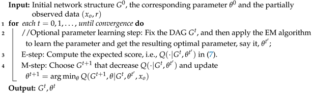 |
To clarify the points of convergence in the SEM algorithm, Friedman [31] defined the class of “stationary points” for the SEM algorithm as all points to which the algorithm can converge. Note that this set of stationary points is a subset of the set of stationary points in spaces of parameterizations of all the candidate Bayesian networks.
Next, we apply the SEM algorithm for structural learning of the censored Gaussian Bayesian Network. We first describe the E-step and M-step in Section 3.2.1 and Section 3.2.2, respectively. Then, we introduce the optional parameter-learning step in Section 3.2.3 and discuss the choice of initial values in Section 3.2.4.
3.2.1. E-Step
According to the density in (3), we compute the expected EBIC score in (7) for complete data
where . Denote
and
then, we obtain
where and is the jth column of B.
Note that, given follows a truncated multivariate normal distribution
where , , is the covariance matrix in the tth iteration, is the vector with element and is the vector with element . Thus, the conditional expectation in (9), (10) and (11) necessitates calculating both the first and second moments of the truncated multivariate normal distribution, which is computationally intensive for moderate size problems as it involves complex numerical integration [42].
To address this issue, we approximate the conditional expectation by the Monte Carlo (MC) sampling of Wei and Tanner [43]. Specifically, we draw a sample of size K from the truncated multivariate normal distribution in (13) by the R package tmvtnorm [44]. This allows us to obtain the complete data where and . Then, we compute approximately and . With these approximations, we can compute the Q function in (9) more efficiently.
3.2.2. M-Step
In the M-step, we aim to search for a DAG G and the corresponding parameters that decrease the Q function. First, we fix G and minimize over , then we obtain
where S is the expected sample covariance matrix with entry being
From (14), we observe that is decomposable with respect to the DAG G, as it is expressed as a sum of local scores, each depending only on a single variable and its parent set. Consequently, any existing score-and-search or hybrid algorithm can be employed to identify an improved structure that further reduces . We recommend using the iterative MCMC (iMCMC) algorithm [17,18] to obtain , as it has been shown to produce higher-quality DAGs compared to Greedy Equivalence Search (GES) [13] and Max-Min Hill-Climbing (MMHC) [15] through simulation studies.
Note that the iMCMC algorithm is a hybrid approach to Bayesian network structure learning that efficiently searches for the maximum a posteriori graph. Unlike traditional MCMC methods, iMCMC first reduces the search space using the PC algorithm or prior knowledge, improving efficiency. It then applies an iterative order MCMC scheme to refine the structure while respecting the learned constraints. Luo et al. [45] adapted iMCMC for Bayesian network structure learning with ordinal data by replacing the posterior score with the BIC score. Following their approach, we use iMCMC to decrease the Q function, which corresponds to the expected EBIC score.
After obtaining , we update the parameter by minimizing . By differentiating with respect to , and , we obtain
where and are the expected sample mean of variable and vector , respectively, and S is the expected sample covariance matrix. The detailed derivation in this subsection will be provided in Appendix A.
3.2.3. Optional Parameter-Learning Step
To implement the EM algorithm in the optional parameter-learning step (i.e., Line 2 of Algorithm 1), we first initialize the parameters using , the estimates obtained from the previous iteration. Then, we iteratively perform the E-step and M-step. The E-step is carried out in the same manner as described in SubSection 3.2.1. In the M-step, we optimize only the parameters while keeping the structure unchanged, unlike the M-step in Section 3.2.2, which searches for an improved network structure.
3.2.4. Initial Values of cSEM
It should be noted that, similar to the EM algorithm, different initial values of in the cSEM algorithm may lead to different outcomes. Therefore, selecting a good initial structure is crucial for achieving robust and accurate results. We propose two alternative initialization strategies for obtaining , using Greedy Equivalence Search (GES) and the iterative MCMC algorithm (iMCMC) [17,18], both of which are widely used for structure learning. Since these algorithms are not designed to handle censored data directly, they are applied to datasets in which the censored values are replaced by their corresponding censoring thresholds. The corresponding initial parameter matrix can be estimated via maximum likelihood estimation (MLE) of Gaussian Bayesian network on the threshold-substituted dataset given . For initializing each and , we assume that each variable follows a normal distribution , and compute the MLEs and by the EM algorithm accordingly.
4. Simulation
In this section, we conduct simulations to assess the performance of the proposed cSEM algorithm in recovering the structure of Bayesian network with censored data. In our simulation, the parameter in of the EBIC score is set to 0.5, following the recommendation of Foygel and Drton [37] for learning Gaussian graphical models. Note that all analyses are performed using R software. Our codes are available at https://github.com/xupf900/cSEM (accessed on 27 April 2025).
In simulation studies of the first two subsections we generate the censored Gaussian dataset as follows. First, we generate a random DAG with a given number of vertices p and an expected neighborhood size s using the randDAG function from the R package pcalg [46]. Second, the sparse adjacency matrix B is obtained from the DAG, where a nonzero entry is drawn uniformly from and . We generate in (3) uniformly from the interval and set for all j. Then, we obtain a multivariate Gaussian distribution as defined by (2). Last, we draw a Gaussian sample from above multivariate Gaussian distribution and cut it by a left-censoring threshold vector l to obtain left-censored data, where l is determined by the mean, the square root of variance of each variable and the percentage c of left censoring.
To assess the performance for structural recovery, we need some metrics. Notice that we can only identify the true DAG up to its Markov equivalence class, so it is more appropriate to compare the corresponding CPDAGs. Therefore, we calculate the Structural Hamming Distance (SHD) between the estimated CPDAG and the true CPDAG. SHD includes the number of extra edges (ee), the number of missing edges (me), the number of reverse directions of edges (rd), the number of missing directions of edges (md), the number of the extra direction of edges (ed). That is, SHD = me + ee + md + ed + rd. We also use the true positive rate (TPR), the false positive rate (FPR) and the true discovery rate (TDR) between the estimated skeleton and the true skeleton. Note that the skeleton of a DAG is an undirected graph with the same vertex set and the undirected edges set where the undirected edge is obtained by removing direction of the directed edge in DAG. TPR is the number of correctly found edges in estimated skeleton divided by the number of true edges in true skeleton, and FPR is the number of incorrectly found edges divided by the number of true gaps in true skeleton and TDR is the number of correctly found edges divided by the number of found edges. To compare the computational efficiency of different algorithms, we record the CPU time for each algorithm.
4.1. Evaluating MC Sampling in E-Step
In this subsection, we evaluate the effect of Monte Carlo (MC) sampling in the E-step of the cSEM algorithm using simulated data. Specifically, we consider a DAG with vertices and 31 edges, and generate a dataset of size , where the proportion of left-censored values is set to . The initial DAG is obtained using the iterative MCMC (iMCMC) algorithm. During the E-step, we vary the MC sampling size K over the values 50, 200, 1000 and 2000. The corresponding variants of the cSEM algorithm are denoted as csem.50, csem.200, csem.1k and csem.2k. Each variant is run fifty times, resulting in fifty CPDAGs per setting.
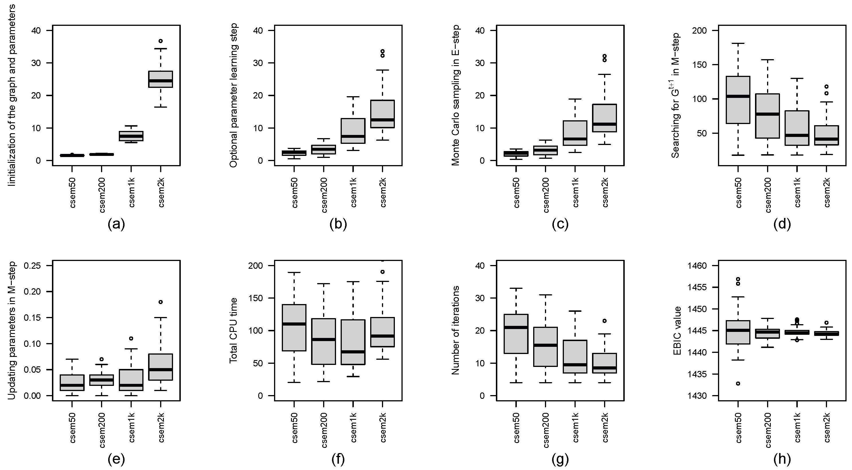
Figure 1 presents boxplots of the CPU time (in seconds) for each computation step, the number of iterations and the EBIC values across the cSEM variants. In addition, Table 1 reports the number of distinct CPDAGs with different SHDs for each value of K. From Figure 1, we observe that, as K increases, the number of iterations required for convergence and the CPU time for searching for in M-step tends to decrease. However, the CPU time spent on initializing the graph and parameters, the optional parameter-learning step, Monte Carlo sampling in E-step and updating parameters in M-step increases with larger K. Notably, the total CPU time does not exhibit a clear trend with respect to K, although results in the shortest total CPU time. In terms of EBIC values, larger K leads to more stable and robust performance, while smaller K (e.g., ) may occasionally yield the lowest EBIC. According to Table 1, the number of distinct CPDAGs generated over fifty runs decreases as K increases: produces eight distinct CPDAGs, while , 1000, and 2000 each result in only two distinct CPDAGs. While achieves the best CPDAG with SHD equal to 0, it also produces the worst with SHD as high as 16. In contrast, larger values of K yield more consistent results, with SHDs ranging between 1 and 5.
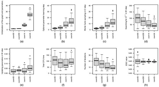
Figure 1.
Boxplots of CPU times in seconds for each step of the cSEM variants across different values of K are presented, including: (a) initialization of the graph and parameters, (b) optional parameter learning step, (c) Monte Carlo sampling in E-step, (d) searching for in M-step, (e) updating parameters in M-step and (f) total computational time. Subfigure (g) shows the boxplot of the number of iterations, and subfigure (h) displays the boxplot of EBIC values for the cSEM variants across different values of K.

Table 1.
Number of distinct CPDAGs for cSEM variants with different K over fifty runs.
These findings suggest that, when computational resources allow for multiple runs, it is beneficial to run csem.50 multiple times and select the CPDAG with the smallest EBIC. However, if only a single run is feasible, using a larger value of K (e.g., or ) is preferable for obtaining more reliable and stable results.
4.2. Comparison of Methods on Data Simulated from Censored GBN
In this subsection, we compare the performance of cSEM with four existing structure learning approaches: the PC-stable algorithm [10] (referred to as PC hereinafter), Greedy Equivalence Search (GES) [13], the iterative MCMC procedure (iMCMC) [17,18] and the Max-Min Hill-Climbing algorithm (MMHC) [15]. Among these methods, PC is a constraint-based approach, GES is a score-and-search method and both iMCMC and MMHC are considered hybrid methods.
For the cSEM algorithm, we evaluate two initialization strategies as described in Section 3.2.4, and we fix the MC sampling size in the E-step to . When the optional parameter-learning step based on the EM algorithm is included, the corresponding versions are denoted by csem.2k.imcmc.emup and csem.2k.ges.emup, depending on whether the initialization is from iMCMC or GES, respectively. If the optional EM-based parameter update is not performed, the versions are referred to as csem.2k.imcmc and csem.2k.ges.
For the PC algorithm, we follow the recommendations in Kalisch and Bühlman [47] and set the significance level . As the performance is generally consistent across these values, we report results only for . For GES and iMCMC, we use the extended BIC (EBIC) with regularization parameter , while for MMHC we use EBIC with , as implemented in the R package bnlearn [48]. Since none of the competing methods are specifically designed to handle censored data, we address censoring by substituting each censored value with its corresponding left-censoring threshold from the vector l. The resulting completed datasets are then passed to the competitors for structure learning. To assess the impact of censoring, we also apply each method to uncensored Gaussian data generated from the same underlying models.
For the simulation setup, we consider vertex numbers and 100, expected neighborhood size , sample sizes and 500, and censoring rates and . For each configuration, we generate 50 random DAGs, and from each DAG we sample an i.i.d. censored dataset of size n. These simulated datasets are used to systematically evaluate and compare the performance of the different structural learning methods.
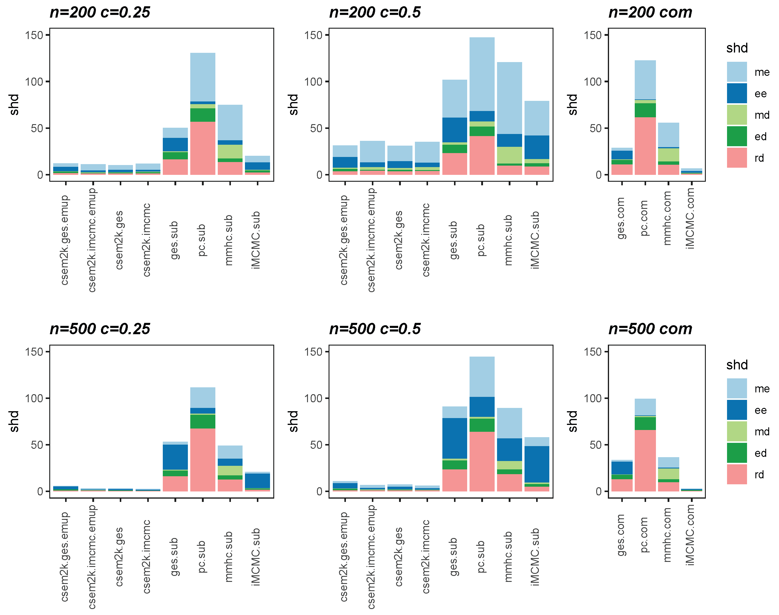
We present the average SHDs using stacked bar charts in Figure 2 and Figure 3, which illustrate the average number of incorrect edges for and , respectively. In these figures, algorithm.sub denotes that an algorithm is applied to a dataset in which censored values are replaced by their corresponding threshold values, while algorithm.com refers to the same algorithm applied to the complete, uncensored Gaussian dataset. From these figures, we observe that different initial DAGs for cSEM result in similar average SHDs. Moreover, the inclusion of the optional parameter-learning step has little effect on the accuracy of structural recovery. However, it can reduce the total CPU time, as detailed in Table A1 in Appendix B. Across all settings, the cSEM variants consistently outperform their algorithm.sub counterparts.

Figure 2.
Stacked bar charts of the average SHDs for .
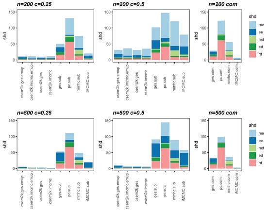
Figure 3.
Stacked bar charts of the average SHDs for .
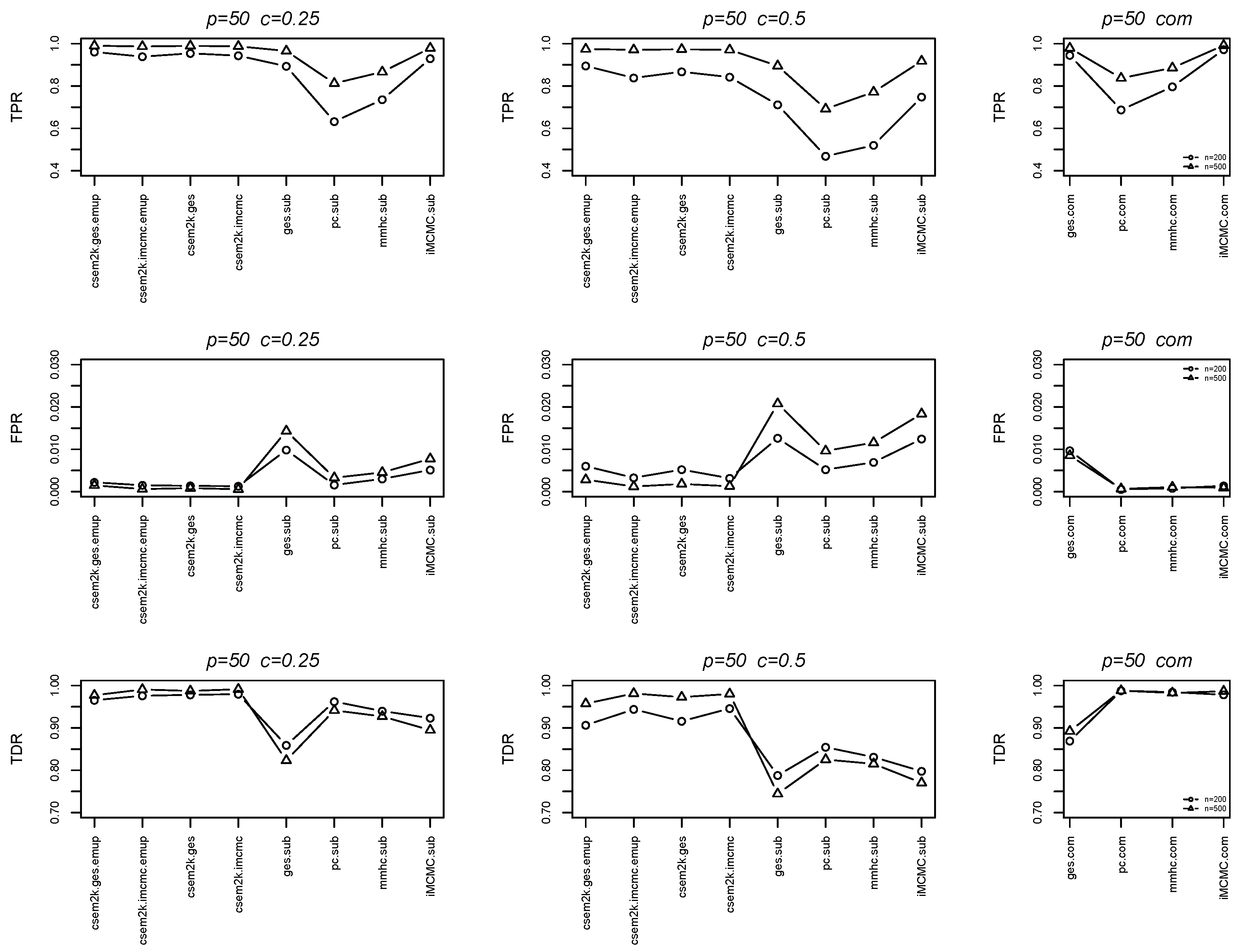
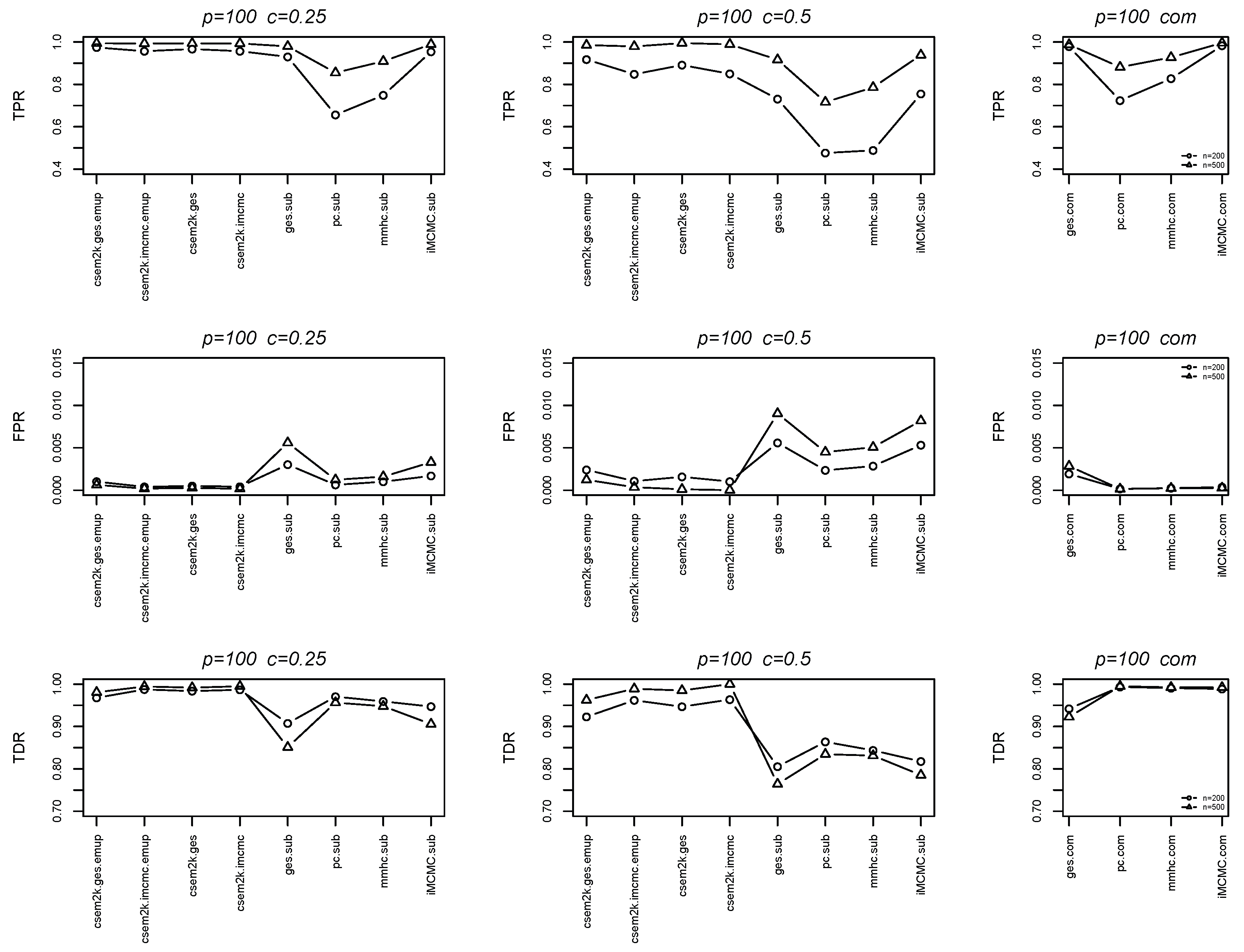
We further report the average true positive rates (TPRs), false positive rates (FPRs) and true discovery rates (TDRs) between the estimated skeletons and the true skeletons in Figure 4 and Figure 5. In each figure, the first, second and third columns correspond to results for , , and the complete dataset, respectively. These figures demonstrate that the cSEM variants outperform all algorithm.sub methods across all three metrics (TPR, FPR and TDR).
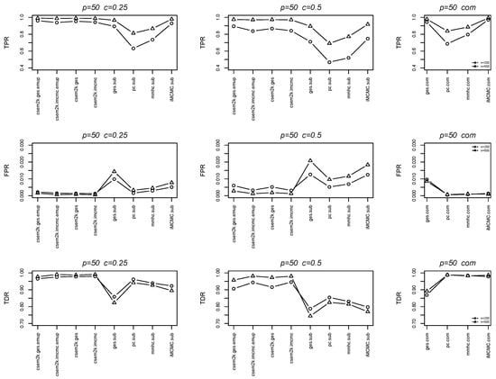
Figure 4.
Line charts of the average TPRs, FPRs and TDRs for .
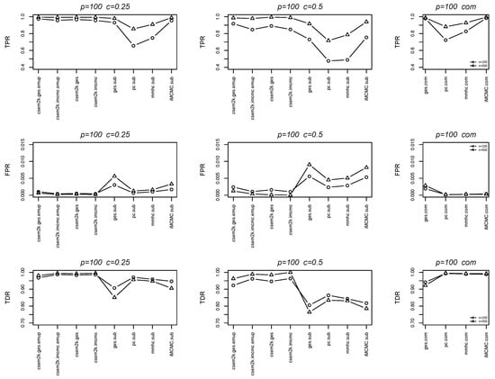
Figure 5.
Line charts of the average TPRs, FPRs and TDRs for .
Detailed information on the average CPU time for all algorithms is provided in the Appendix B.
4.3. Additional Simulations on Artificially Censored Biological Data
In this subsection, we assess the performance of our cSEM algorithm using realistic biological data from the New Hampshire Birth Cohort Study, as provided by Ma et al. [49]. The dataset is available at https://doi.org/10.21228/M8K69N (accessed on 18 May 2024). It comprises metabolomics data obtained from stool samples collected from infants at around 6 weeks of age, encompassing information on 36 metabolites from a total of 158 infants.
Despite the data being fully observed, we apply our method to the datasets where observations are made artificially right-censored similarly to Augugliaro et al. [25]. Three datasets are generated with varying percent c of right-censoring by designating the top 10%, 20% and 30% of the highest values to be censored. To assess our method, we compare it with k-nearest neighbor imputation (denoted as missknn) and random forests imputation (denoted as missforest). Both techniques start by imputing censored values and then utilize iMCMC to learn structure. In Table 2, the structural Hamming distance (SHD) and mean square error (MSE) of cSEM, missforest and missknn are presented under varying degrees of censoring. The MSE evaluates the estimation precision of the covariance matrix, calculated as , where is the covariance matrix computed from the estimated adjacency matrix by the iMCMC method for complete data, and is the covariance matrix obtained by cSEM variants with different K and initial values, missknn or missforest. All cSEM variants consistently outperform two imputation methods in terms of structural learning and parameter estimation across various censoring degrees. However, the CPDAGs obtained from cSEM variants with different values of K and different initializations may vary and exhibit some instability. This suggests that running cSEM multiple times and selecting the CPDAG with the smallest EBIC value can lead to more reliable results.
Table 2.
SHDs and MSEs of cSEM variants, missforest and missknn under and .
5. Structural Learning of Single Cell Data
In a study on blood cell formation, Psaila et al. [50] identified three distinct subpopulations of cells that hematopoietic stem cells can generate through cellular differentiation; one of them is called MK-MEP. This subpopulation is a rare population of cells and it mainly generates megakaryocyte progeny. In this section, our cSEM algorithm is applied to model networks from a dataset comprising single human MK-MEP cells and genes that is available from Augugliaro et al. [25]. Data were obtained by multiplex RT-qPCR analysis. RT-qPCR measures gene expression by amplifying DNA sequences. If a target gene is not expressed, the expression level does not reach the set threshold within the maximum cycles, making the cycle-threshold value undefined. This leads to right-censored data. In this dataset, the limit of detection is fixed by the manufacturer to 40, which means that gene expressions are right-censored at 40.
In this application, we assume that the maximum number of parents for each variable is less than the sample size to ensure that the sub-matrix of the expected sample covariance matrix is invertible in Equations (14) and (16). We run csem.50.ges and csem.50.iMCMC fifty times each. The smallest EBIC value achieved by csem.50.ges is 4750.352, while that of csem.50.iMCMC is 4767.84. Therefore, we present the CPDAG corresponding to the smallest EBIC from csem.50.ges in Figure 6. Among the 63 variables, only the 22 connected by at least one edge are shown in the figure. The directed edge implies the direct dependency relationship between the child variable and parent variable. The presence of undirected edges, such as those between CD9 and CNRIP1, and between HIF1A and RGS18, indicates that the directionality of these relationships cannot be determined from the data. As illustrated in Figure 6, TGFB1, VWF and CD61 occupy central positions in the inferred network. TGFB1 is a multifunctional cytokine that plays a key role in numerous cellular physiological processes, including cell growth, differentiation, apoptosis, immunomodulation and extracellular matrix synthesis. VWF and CD61 are highly expressed in the MK-MEP subpopulation. VWF is involved in blood coagulation and platelet aggregation, while CD61 plays an important role in platelet generation and hematopoietic stem cell function. This structural analysis of single human MK-MEP cells using cSEM serves as a reference for genetic scientists.
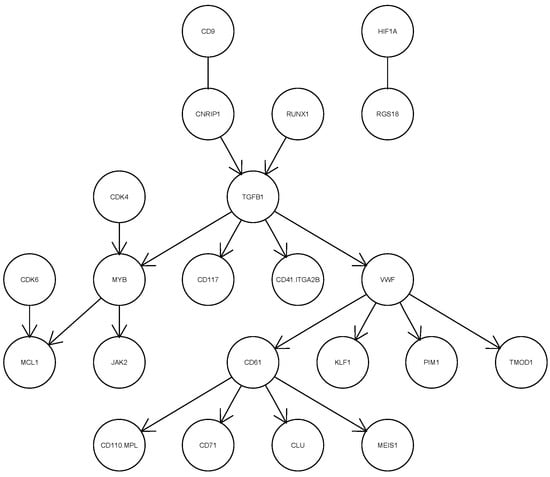
Figure 6.
Estimated CPDAG of the network with the smallest EBIC for single human MK-MEP cells.
6. Conclusions
In this paper, we define the censored GBN, and propose the cSEM algorithm for learning Bayesian networks from censored data by combining the MC sampling method [43] and the Structural EM algorithm [31]. By extensive simulation studies, we demonstrate the computational efficiency of MC sampling in E-step of cSEM and we show that the cSEM algorithm outperforms all competitors, including PC, GES, iMCMC and MMHC, in recovering the network structure. To validate its real-world applicability, we apply cSEM to the MK-MEP human cell dataset, revealing key regulatory networks involved in blood development—offering valuable insights for genetic research.
In the future, we will explore several directions to enhance our approach. First, while cSEM is effective, it is computationally expensive, primarily due to the iMCMC algorithm used in the M-step, which is time-consuming. A potential improvement is to incorporate more efficient score-and-search methods [8,51] to enhance computational efficiency. Second, we will extend our work to structure learning in high-dimensional censored data, where the number of variables exceeds the sample size. In this setting, -penalty, SCAD penalty and MCP penalty have proven effective for Bayesian network structure learning with complete data [39,40]. A natural extension is to apply the EM algorithm to optimize the penalized log-likelihood for censored data using these penalties. However, rigorous convergence analysis will be necessary to ensure the stability and reliability of this approach.
Author Contributions
Conceptualization, P.-F.X., S.L., Q.-Z.Z. and M.-L.T.; Funding acquisition, P.-F.X.; Methodology, P.-F.X. and S.L.; Software, P.-F.X. and S.L.; Writing—original draft, P.-F.X., S.L. and Q.-Z.Z.; Writing—review and editing, P.-F.X., S.L., Q.-Z.Z. and M.-L.T. All authors have read and agreed to the published version of the manuscript.
Funding
The research of Ping-Feng Xu was supported by the National Social Science Fund of China (No. 23BTJ062).
Data Availability Statement
Data are available upon request to the authors.
Conflicts of Interest
The authors declare no conflicts of interest.
Appendix A. Detailed Derivations in M-Step
In this appendix, we derive (14)–(17) in M-step. Denote being the expected mean with the jth element being , and S be the expected sample covariance matrix with the entry being
Note that, , where is independent for . We fix G and differentiate with respect to and set to zero; then, we obtain
From (A1), (A2) and (A3), we obtain
Appendix B. Average CPU Time
Table A1 summarizes the average CPU time (in seconds) of each step, average CPU time in total and average number of iterations of cSEM variants and average CPU time of iMCMC, GES, MMHC, PC for . From this table, we observe that incorporating the optional parameter-learning step enhances convergence speed by reducing the number of iterations. It leads to a reduction in total CPU time, although the parameter-learning step introduces additional computational overhead. In addition, due to the iterative nature of cSEM, cSEM variants are slower than all competitors. Such a loss in computational efficiency is mainly due to the iterative search process for the DAG by iMCMC in M-step. From Table A1, it can be seen that iMCMC exhibits slower computational efficiency compared to PC, MMHC and GES, all of which are similar in CPU time. In the future, we will try to incorporate more efficient score-and-search methods [8,51] to improve computational efficiency.
Table A1.
Average CPU time (in seconds) of each step, average CPU time in total and average number of iterations of cSEM variants and four competitors.
Table A1.
Average CPU time (in seconds) of each step, average CPU time in total and average number of iterations of cSEM variants and four competitors.
| c = 0.25 | c = 0.5 | com | |||||||||||
|---|---|---|---|---|---|---|---|---|---|---|---|---|---|
| EM.update | E.step | M.step | Total | Iter | EM.update | E.step | M.step | Total | Iter | Total | |||
| p = 50 | n = 200 | csem50.ges.emup | 11.38 | 10.19 | 131.10 | 153.03 | 17.08 | 26.61 | 22.86 | 153.96 | 204.02 | 20.08 | |
| csem50.imcmc.emup | 12.19 | 11.05 | 141.25 | 167.18 | 19.30 | 23.57 | 21.31 | 138.31 | 186.13 | 19.98 | |||
| csem50.ges | 0.00 | 13.60 | 178.98 | 192.94 | 22.78 | 0.00 | 32.38 | 213.27 | 246.24 | 29.54 | |||
| csem50.imcmc | 0.00 | 13.08 | 173.22 | 189.04 | 22.32 | 0.00 | 32.74 | 213.42 | 249.11 | 30.66 | |||
| ges | 0.10 | 0.08 | 0.16 | ||||||||||
| pc | 0.08 | 0.06 | 0.09 | ||||||||||
| mmhc | 0.10 | 0.10 | 0.10 | ||||||||||
| iMCMC | 7.76 | 7.57 | 7.53 | ||||||||||
| n = 500 | csem50.ges.emup | 26.98 | 24.12 | 126.75 | 178.43 | 15.60 | 64.30 | 52.64 | 146.22 | 264.27 | 18.52 | ||
| csem50.imcmc.emup | 27.45 | 24.65 | 132.85 | 187.85 | 17.00 | 62.33 | 54.44 | 152.43 | 272.63 | 19.82 | |||
| csem50.ges | 0.00 | 29.68 | 157.77 | 188.06 | 19.74 | 0.00 | 86.22 | 245.03 | 332.40 | 30.44 | |||
| csem50.imcmc | 0.00 | 31.82 | 171.69 | 206.50 | 21.60 | 0.00 | 80.91 | 232.69 | 317.17 | 29.04 | |||
| ges | 0.12 | 0.12 | 0.17 | ||||||||||
| pc | 0.15 | 0.16 | 0.14 | ||||||||||
| mmhc | 0.14 | 0.14 | 0.15 | ||||||||||
| iMCMC | 9.09 | 10.49 | 7.87 | ||||||||||
| p = 100 | n = 200 | csem50.ges.emup | 22.89 | 20.56 | 658.80 | 715.40 | 17.34 | 126.91 | 103.92 | 695.10 | 929.27 | 17.78 | |
| csem50.imcmc.emup | 22.72 | 20.40 | 600.17 | 655.79 | 17.34 | 105.08 | 88.42 | 577.90 | 785.19 | 16.10 | |||
| csem50.ges | 0.00 | 22.58 | 694.62 | 718.74 | 18.74 | 0.00 | 163.38 | 1107.90 | 1274.56 | 28.90 | |||
| csem50.imcmc | 0.00 | 25.05 | 765.48 | 803.26 | 21.44 | 0.00 | 145.89 | 984.50 | 1144.85 | 26.42 | |||
| ges | 0.43 | 0.40 | 0.50 | ||||||||||
| pc | 0.19 | 0.15 | 0.21 | ||||||||||
| mmhc | 0.33 | 0.33 | 0.33 | ||||||||||
| iMCMC | 36.60 | 38.54 | 35.43 | ||||||||||
| n = 500 | csem50.ges.emup | 45.15 | 39.43 | 494.57 | 581.10 | 12.88 | 126.91 | 103.92 | 695.10 | 929.27 | 17.78 | ||
| csem50.imcmc.emup | 43.27 | 37.66 | 473.67 | 567.26 | 13.10 | 105.08 | 88.42 | 577.90 | 785.19 | 16.10 | |||
| csem50.ges | 0.00 | 54.44 | 700.19 | 756.62 | 18.26 | 0.00 | 163.38 | 1107.90 | 1274.56 | 28.90 | |||
| csem50.imcmc | 0.00 | 57.86 | 754.20 | 825.35 | 19.96 | 0.00 | 145.89 | 984.50 | 1144.85 | 26.42 | |||
| ges | 0.51 | 0.56 | 0.53 | ||||||||||
| pc | 0.39 | 0.38 | 0.38 | ||||||||||
| mmhc | 0.45 | 0.44 | 0.45 | ||||||||||
| iMCMC | 41.80 | 53.31 | 36.43 | ||||||||||
References
- Needham, C.J.; Bradford, J.R.; Bulpitt, A.J.; Westhead, D.R. BA primer on learning in Bayesian networks for computational biology. PLoS Comput. Biol. 2007, 3, e129. [Google Scholar] [CrossRef] [PubMed]
- Agrahari, R.; Foroushani, A.; Docking, T.R.; Chang, L.; Duns, G.; Hudoba, M.; Karsan, A.; Zare, H. Applications of Bayesian network models in predicting types of hematological malignancies. Sci. Rep. 2018, 8, 6951. [Google Scholar] [CrossRef]
- Pearl, J. Probabilistic Reasoning in Intelligent Systems: Networks of Plausible Inference, 2nd ed.; Morgan Kaufmann: San Francisco, CA, USA, 1988. [Google Scholar]
- Zhang, H.; Jiang, L.; Zhang, W.; Li, C. Multi-view attribute weighted naive Bayes. IEEE Trans. Knowl. Data Eng. 2023, 35, 7291–7302. [Google Scholar] [CrossRef]
- Zhang, H.; Jiang, L.; Yu, L. Attribute and instance weighted naive Bayes. Pattern Recognit. 2021, 111, 107674. [Google Scholar] [CrossRef]
- Liu, F.; Zhang, S.W.; Guo, W.F.; Wei, Z.G.; Chen, L. Inference of gene regulatory network based on local Bayesian networks. PLoS Comput. Biol. 2016, 12, e1005024. [Google Scholar] [CrossRef] [PubMed]
- Han, S.W.; Chen, G.; Cheon, M.S.; Zhong, H. Estimation of directed acyclic graphs through two-stage adaptive lasso for gene network inference. J. Am. Stat. Assoc. 2016, 111, 1004–1019. [Google Scholar] [CrossRef]
- Kitson, N.K.; Constantinou, A.C.; Guo, Z.; Liu, Y.; Chobtham, K. A survey of Bayesian network structure learning. Artif. Intell. Rev. 2023, 56, 8721–8814. [Google Scholar] [CrossRef]
- Spirtes, P.; Glymour, C. An algorithm for fast recovery of sparse causal graphs. Soc. Sci. Comput. Rev. 1991, 9, 62–72. [Google Scholar] [CrossRef]
- Colombo, D.; Maathuis, M.H. Order-independent constraint-based causal structure learning. J. Mach. Learn. Res. 2014, 15, 3921–3962. [Google Scholar]
- Colombo, D.; Maathuis, M.H.; Kalisch, M.; Richardson, T.S. Learning high-dimensional directed acyclic graphs with latent and selection variables. Ann. Stat. 2012, 40, 294–321. [Google Scholar] [CrossRef]
- Marella, D.; Vicard, P. Bayesian network structural learning from complex survey data: A resampling based approach. Stat. Methods Appl. 2022, 31, 981–1013. [Google Scholar] [CrossRef]
- Chickering, D.M. Optimal structure identification with greedy search. J. Mach. Learn. Res. 2002, 3, 507–554. [Google Scholar]
- Moffa, G. Partition MCMC for inference on acyclic digraphs. J. Am. Stat. Assoc. 2017, 112, 282–299. [Google Scholar]
- Tsamardinos, I.; Brown, L.E.; Aliferis, C.F. The max-min hill-climbing Bayesian network structure learning algorithm. Mach. Learn. 2006, 65, 31–78. [Google Scholar]
- Gasse, M.; Aussem, A.; Elghazel, H. A hybrid algorithm for Bayesian network structure learning with application to multi-label learning. Expert Syst. Appl. 2014, 41, 6755–6772. [Google Scholar] [CrossRef]
- Kuipers, J.; Suter, P.; Moffa, G. Efficient sampling and structure learning of Bayesian networks. J. Comput. Graph. Stat. 2022, 31, 639–650. [Google Scholar] [CrossRef]
- Suter, P.; Kuipers, J.; Moffa, G.; Beerenwinkel, N. Bayesian structure learning and sampling of Bayesian networks with the R Package BiDAG. J. Stat. Softw. 2023, 105, 1–31. [Google Scholar] [CrossRef]
- Song, J.; Barnhart, H.X.; Lyles, R.H. A GEE approach for estimating correlation coefficients involving left-censored variables. J. Data Sci. 2004, 2, 245–257. [Google Scholar] [CrossRef]
- Lee, G.; Scott, C. EM algorithms for multivariate Gaussian mixture models with truncated and censored data. Comput. Stat. Data Anal. 2012, 56, 2816–2829. [Google Scholar]
- Perkins, N.J.; Schisterman, E.F.; Vexler, A. Multivariate normally distributed biomarkers subject to limits of detection and receiver operating characteristic curve inference. Acad. Radiol. 2013, 20, 838–846. [Google Scholar] [CrossRef]
- Hoffman, H.J.; Johnson, R.E. Pseudo-likelihood estimation of multivariate normal parameters in the presence of left-censored data. J. Agric. Biol. Environ. Stat. 2015, 20, 156–171. [Google Scholar]
- Jones, M.P.; Perry, S.S.; Thorne, P.S. Maximum pairwise pseudo-likelihood estimation of the covariance matrix from left-censored data. J. Agric. Biol. Environ. Stat. 2015, 20, 83–99. [Google Scholar] [PubMed]
- Pesonen, M.; Pesonen, H.; Nevalainen, J. Covariance matrix estimation for left-censored data. Comput. Stat. Data Anal. 2015, 92, 13–25. [Google Scholar]
- Augugliaro, L.; Abbruzzo, A.; Vinciotti, V. ℓ1-penalized censored Gaussian graphical model. Biostatistics 2020, 21, e1–e16. [Google Scholar]
- Augugliaro, L.; Sottile, G.; Vinciotti, V. The conditional censored graphical lasso estimator. Stat. Comput. 2020, 30, 1273–1289. [Google Scholar]
- Sottile, G.; Augugliaro, L.; Vinciotti, V. The joint censored Gaussian graphical lasso model. In SIS 2022 Book of the Short Papers; Università degli Studi di Palermo: Palermo, Italy, 2022; pp. 1829–1834. [Google Scholar]
- Koller, D.; Friedman, N. Probabilistic Graphical Models: Principles and Techniques; The MIT Press: London, UK, 2009. [Google Scholar]
- Geiger, D.; Heckerman, D. Parameter priors for directed acyclic graphical models and the characterization of several probability distributions. Ann. Stat. 2002, 30, 1412–1440. [Google Scholar] [CrossRef]
- Moffa, G.; Heckerman, D. Addendum on the scoring of Gaussian directed acyclic graphical models. Ann. Stat. 2014, 42, 1689–1691. [Google Scholar]
- Friedman, N. Learning belief networks in the presence of missing values and hidden variables. In Proceedings of the 14th International Confeerence on Machine Learning, Nashville, TN, USA, 8–12 July 1997; pp. 125–133. [Google Scholar]
- Friedman, N. The Bayesian structural EM algorithm. In Proceedings of the 14th Conference on Uncertainty in Artifical Intelligence, Madison, WI, USA, 24–26 July 1998; pp. 129–138. [Google Scholar]
- Lauritzen, S.L. Graphical Models; Oxford Statistical Sience Series; Clarendon Press: Oxford, UK, 1996. [Google Scholar]
- Shojaie, A.; Michailidis, G. Penalized likelihood methods for estimation of sparse high-dimensional directed acyclic graphs. Biometrika 2010, 97, 519–538. [Google Scholar] [CrossRef]
- Little, R.J.A.; Rubin, D.B. Statistical Analysis with Missing Data, 3rd ed.; John Wiley & Sons: Hoboken, NJ, USA, 2019. [Google Scholar]
- Chen, J.; Chen, Z. Extended Bayesian information criteria for model selection with large model spaces. Biometrika 2008, 95, 759–771. [Google Scholar] [CrossRef]
- Foygel, R.; Drton, M. Extended Bayesian information criteria for Gaussian graphical models. In Proceedings of the 24th International Conference on Neural Information Processing Systems, Vancouver, Canada, 6–9 December 2010; pp. 604–612. [Google Scholar]
- Scutari, M.; Graafland, C.E.; Gutiérrez, J.M. Who learns better Bayesian network structures: Accuracy and speed of structure learning algorithms. Int. J. Approx. Reason. 2019, 115, 235–253. [Google Scholar] [CrossRef]
- Fu, F.; Zhou, Q. Learning sparse causal Gaussian networks with experimental intervention: Regularization and coordinate descent. J. Am. Stat. Assoc. 2013, 108, 288–300. [Google Scholar]
- Aragam, B.; Zhou, Q. Concave penalized estimation of sparse Gaussian Bayesian networks. J. Mach. Learn. Res. 2015, 16, 2273–2328. [Google Scholar]
- Dempster, A.P.; Laird, N.M.; Rubin, D.B. Maximum likelihood from incomplete data via the EM algorithm. J. R. Stat. Soc. Ser. B (Methodol.) 1977, 39, 1–38. [Google Scholar]
- Genz, A.; Bretz, F. Computation of Multivariate Normal and t Probabilities; Springer: Berlin, Germany, 2009. [Google Scholar]
- Wei, G.G.; Tanner, M.A. A Monte Carlo implementation of the EM algorithm and the poor man’s data augmentation algorithms. J. Am. Stat. Assoc. 1990, 85, 699–704. [Google Scholar]
- Wilhelm, S.; Manjunath, B.G. tmvtnorm: Truncated Multivariate Normal and Student t Distribution, version 1.5. 2022. Available online: https://cran.r-project.org/web/packages/tmvtnorm/index.html (accessed on 10 February 2024).
- Luo, X.G.; Moffa, G.; Kuipers, J. Learning Bayesian networks from ordinal data. J. Mach. Learn. Res. 2021, 22, 1–44. [Google Scholar]
- Kalisch, M.; Mächler, M.; Colombo, D.; Maathuis, M.H.; Bühlmann, P. Causal inference using graphical models with the R package pcalg. J. Stat. Softw. 2012, 47, 1–26. [Google Scholar] [CrossRef]
- Kalisch, M.; Bühlman, P. Estimating high-dimensional directed acyclic graphs with the PC-algorithm. J. Mach. Learn. Res. 2007, 8, 613–636. [Google Scholar]
- Scutari, M. Learning Bayesian networks with the bnlearn R Package. J. Stat. Softw. 2010, 35, 1–22. [Google Scholar] [CrossRef]
- Ma, J.; Shojaie, A.; Michailidis, G. Network-based pathway enrichment analysis with incomplete network information. Bioinformatics 2016, 32, 3165–3174. [Google Scholar] [CrossRef]
- Psaila, B.; Barkas, N.; Iskander, D.; Roy, A.; Anderson, S.; Ashley, N.; Caputo, V.S.; Lichtenberg, J.; Loaiza, S.; Bodine, D.M.; et al. Single-cell profiling of human megakaryocyte-erythroid progenitors identifies distinct megakaryocyte and erythroid differentiation pathways. Genome Biol. 2016, 17, 1–19. [Google Scholar] [CrossRef]
- Vowels, M.J.; Camgoz, N.C.; Bowden, R. D’ya like dags? A survey on structure learning and causal discovery. ACM Comput. Surv. 2022, 55, 1–36. [Google Scholar] [CrossRef]


Disclaimer/Publisher’s Note: The statements, opinions and data contained in all publications are solely those of the individual author(s) and contributor(s) and not of MDPI and/or the editor(s). MDPI and/or the editor(s) disclaim responsibility for any injury to people or property resulting from any ideas, methods, instructions or products referred to in the content. |
© 2025 by the authors. Licensee MDPI, Basel, Switzerland. This article is an open access article distributed under the terms and conditions of the Creative Commons Attribution (CC BY) license (https://creativecommons.org/licenses/by/4.0/).