Article

Inverse Problem of Identifying a Time-Dependent Source Term in a Fractional Degenerate Semi-Linear Parabolic Equation

by
Maroua Nouar
1,
Chattouh Abdeledjalil
1,
Omar Mossa Alsalhi
2 and
Hamed Ould Sidi
3,*
1
Departement of Mathematics, Abbes Laghrour University Khenchela, Khenchela 40004, Algeria
2
Department of Mathematics, Al-Leith University College, Umm Al-Qura University, Mecca 21961, Saudi Arabia
3
Département des Méthodes Quantitatives et Informatiques, Institut Supérieur de Comptabilité et d’Administration des Entreprises (ISCAE), Nouakchott 6093, Mauritania
*
Author to whom correspondence should be addressed.
Mathematics 2025, 13(9), 1486; https://doi.org/10.3390/math13091486
Submission received: 2 April 2025 / Revised: 25 April 2025 / Accepted: 26 April 2025 / Published: 30 April 2025
(This article belongs to the Special Issue Inverse Problems and Numerical Computation in Mathematical Physics)

Abstract

:
This work investigates the inverse problem of identifying a time-dependent source term in a time-fractional semi-linear degenerate parabolic equation using integral measurement data. We establish the unique solvability of the inverse problem within a suitable functional framework. The proof methodology is based on the Rothe method, where the variational formulation is discretized in time, and a priori estimates for discrete solutions are derived. These estimates are then utilized to demonstrate the convergence of Rothe approximations to a unique weak solution. Additionally, we develop a numerical scheme based on the L 1 -Galerkin finite element method, combined with iterative refinement, to reconstruct the unknown source term. The numerical performance of the proposed method is validated through a series of computational experiments, demonstrating its stability and robustness against noisy data.

1. Introduction

Inverse problems, particularly those involving the identification of source terms in systems governed by time-fractional partial differential equations (PDEs), have garnered significant attention due to their wide-ranging practical applications. Time-fractional PDEs, which generalize classical integer–order models, are particularly useful in describing processes that exhibit memory effects or anomalous behavior, such as non-local interactions or long-range dependencies in time. These features are commonly observed in various real-world phenomena, including diffusion processes in heterogeneous media, viscoelasticity, and wave propagation in complex materials.
Our objective through this work is to handle the inverse problem of recovering a time-dependent source term in a time-fractional semi-linear degenerate parabolic equation. More precisely, let us consider the following problem:
D t α θ ( a ( x ) θ x ) x = F ( θ , x , t ) + p ( x ) r ( t ) , x Ω , t ( 0 , T ) ,
subject to the initial and boundary conditions
θ ( 0 , t ) = θ ( 1 , t ) = 0 , t ( 0 , T ) , θ ( x , 0 ) = θ 0 ( x ) , x Ω ,
where Ω = ( 0 , 1 ) stands for the spatial domain, 0 < T < + is a given fixed final time, D t α denotes the Caputo fractional left-derivative of order 0 < α < 1 with respect to time variable t, and it is defined by
D t α θ ( · , t ) : = 1 Γ ( 1 α ) 0 t ( t s ) α s θ ( · , s ) d s , 0 < t < T ,
where Γ ( · ) is the Gamma function defined for z C , with the positive real part ( z ) > 0 as
Γ ( z ) = 0 s z 1 e s d s , ( z ) > 0 .
As to the nonlinearity, we suppose that F is subject to the following condition:
| F ( ϑ 1 , x , t ) F ( ϑ 2 , x , t ) | γ ( x , t ) | ϑ 1 ϑ 2 | , ϑ 1 , ϑ 2 [ M 0 , M 0 ] ,
where M 0 is a priori known real number and γ L 2 ( Ω × ( 0 , T ) ) is a bounded function with γ L γ 0 .
The diffusion coefficient a ( x ) is typically assumed to be a strictly positive and continuous function on the interval [ 0 , 1 ] . However, if  a ( x ) vanishes at certain points within the domain Ω or on its boundaries, the corresponding differential equation becomes degenerate. Specifically, Problem (1) is referred to as a weakly degenerate problem if a ( x ) vanishes at the boundary (e.g., at  x 0 = 0 ) and satisfies
a C ( [ 0 , 1 ] ) C 1 ( ( 0 , 1 ] ) , a ( 0 ) = 0 , and a ( x ) > 0 for x ( 0 , 1 ] , κ [ 0 , 1 ) such that x a ( x ) κ a ( x ) , x [ 0 , 1 ] .
A typical example of the weak degenerate diffusion coefficient is a ( x ) = x η with η ( 0 , 1 ) .
Few results are available in the literature, despite the fact that numerous application-driven problems are governed by parabolic equations that degenerate at the boundary of the spatial domain. Notably, several studies, such as those in [1,2,3], provide insights into this class of equations. A particularly relevant example is the Crocco-type equation, which arises in the analysis of the velocity field of a laminar flow over a flat plate.
To compensate for the incomplete data about r ( t ) , an additional condition is given in the form of a weighted average of θ on a subdomain ω Ω , which is expressed as follows:
ω ψ ( x ) θ ( x , t ) d x = E ( t ) ,
where we claim that ψ H 0 1 ( ω ) and x 0 ω ¯ . The choice of measuring over the domain ω , with  x 0 ω , is physically reasonable. From a physical perspective, the diffusion coefficient a ( x ) is generally assumed to be positive and bounded, ensuring that the physical process whether it is heat conduction, particle diffusion, or any other form of transport proceeds in a regular and stable manner across the domain. Consequently, the exclusion of x 0 from ω ¯ guarantees that the diffusion process within the domain ω ¯ remains free of singularities or degeneracies since the diffusion coefficient a ( x ) is strictly positive over ω .
Inverse problems for partial differential equations, focusing on identifying and reconstructing unknown terms or parameters, lie at the heart of numerous scientific and engineering practical applications, such as reconstructing internal body structures from imaging data in medicine [4], identifying sources of pollution in environmental science [5,6], determining properties of materials in engineering [7], identifying mineral deposits [8], oil and gas reservoirs [9], and so on.
Time-fractional partial differential equations have emerged as models that are characterized by being versatile and effective for describing processes with memory effects and anomalous diffusion, such as sub-diffusion in porous media [10], viscoelastic behavior of polymers [11], and anomalous diffusion in biological systems [12].
There exists a significant corpus of research and works addressing inverse source problems related to boundary value problems governed by parabolic equations, ranging from parabolic equations of integer order, with and without degeneracy, to their counterparts involving fractional derivatives (see, e.g., Ref. [13,14,15,16,17,18,19,20,21]). In particular, inverse problems related to identifying time-dependent parameters or source terms in integer–order parabolic systems have been extensively studied. Some previous studies have used the Rothe method to address the source identification problem for various parabolic systems. For example, Grimmonprez and Slodička [22] investigated the inverse problem of reconstructing an unknown time-dependent source parameter in a semi-linear parabolic equation. The work in  [23] is devoted to studying the inverse problem of identifying an unknown time-dependent memory kernel in a semi-linear integro-differential parabolic equation. The Rothe method involves discretizing the time variable first, transforming the original parabolic problem into a sequence of elliptic boundary value problems. By solving these elliptic problems sequentially, one can construct a solution for the initial parabolic problem (for an overview of this method, refer to [24,25]). The same approach has been applied to identify the time-dependent component of the source term in fractional parabolic equations, considering various boundary conditions and additional measurements [26].
In the same context, regularization methods, in their various forms, have been among the most effective tools for studying such problems. The most representative method is the Tikhonov regularization method (TRM), which is considered one of the most effective regularization techniques for addressing the instability inherent in such problems. For example, in [27], (TRM) has been used to solve the inverse source problem for a multi-dimensional time-fractional diffusion equation from boundary Cauchy data. On the same line, Ruan and Wang have addressed in [28] the inverse problem of reconstructing a time-dependent term source in a fractional time diffusion equation using (TRM). In a recent paper [29], the authors investigated the inverse problem of identifying a time-independent source term in a fractional Rayleigh–Stokes equation, by using a fractional Tikhonov regularization method.
Certainly, there are alternative strategies to achieve the regularization. Wei and Wang [30] employed a modified quasi-boundary value method (QBV) to regularize an inverse source problem for a fractional diffusion model and proved convergence rate results for the approximate solution. In [31], the authors presented a modified approach (QBV) for the study of an inverse source problem for the time-fractional diffusion equation. The total-variation regularization method was used in [32] to handle an inverse problem of recovering an unknown diffusion coefficient in a parabolic equation. The work in  [33] proposed the Carleman-weighted convexification method for a parabolic coefficient identification problem. Lv and Feng [34] used a mollification regularization method based on a bilateral exponential to recover simultaneously a space-dependent source problem and the initial value for a time-fractional diffusion-wave equation. Iterative regularization methods were also employed and further developed both theoretically and numerically, such as the conjugate gradient method [35,36], Landweber-type methods [37], and the Levenberg–Marquardt method [38], among others.
Considering the literature on this topic, it is evident that significant effort has been devoted and numerous studies have been conducted to comprehensively address inverse problems from all possible perspectives, which is evidenced by the diversity of the studied problems, reflecting the broad scope and depth of research dedicated to this field. However, the interplay of fractional derivatives, degeneracy, and nonlinearity remains under-explored, leaving a critical gap in the theory of inverse problems from both theoretical and numerical aspects.
Motivated by these considerations, the primary objective of this work is to bridge this gap by rigorously studying the inverse problem of recovering a time-dependent source term r ( t ) in a time-fractional degenerate semi-linear parabolic equation. This study makes two key contributions. First, we establish the unique solvability of the inverse problem using the Rothe method. By handling fractional derivatives through Riemann–Liouville kernels and leveraging compact embeddings in weighted Sobolev spaces, we extend the existence and uniqueness results obtained in [26] to a time-fractional reaction–diffusion problem with the presence of a boundary degeneracy. Secondly, from a computational perspective, we designed a numerical method using the L 1 -Galerkin finite element method for the full discretization of the problem, combined with an iterative refinement algorithm, to numerically reconstruct the unknown source term r ( t ) . The scheme robustness against noisy data and nonlinearities is demonstrated through several numerical tests. It is noteworthy that the inverse problem addressed in this study is accompanied by a measurement condition over a subdomain ω , which presents an additional mathematical challenge in deriving theoretical results or applying numerical methods. However, from a physical standpoint, this approach is more practical, as obtaining measurements over a subdomain ω is often more feasible than over the entire domain Ω .
This paper is structured as follows. Section 2 presents preliminary mathematical tools, including weighted Sobolev spaces and properties of the Riemann–Liouville kernel, which are essential for the subsequent sections. In Section 3, we formulate the inverse problem in a variational framework, derive the weak solution, and rigorously prove uniqueness using energy estimates. Section 4 employs the Rothe method to discretize the problem in time, derive a priori estimates for discrete solutions, and construct convergent Rothe functions to establish existence. For the numerical aspect, Section 5 details an L 1 -Galerkin finite element scheme combined with iterative refinement to reconstruct the source term, validated through a series of numerical tests. Finally, the last section provides a brief conclusion with remarks and potential extensions.

2. Preliminaries

2.1. Functional Spaces

In this subsection, we introduce some functional spaces used throughout this work, in particular, weighted Sobolev spaces associated with the degenerate coefficient a ( x ) . Let us define
H a 1 ( Ω ) : = φ L 2 ( Ω ) : φ abs . cont . in [ 0 , 1 ] , a φ x L 2 ( Ω ) , φ ( 0 ) = φ ( 1 ) = 0 ,
which is a Hilbert space with respect to the scalar product and its associated norm
φ , ψ 1 , a : = Ω φ ψ + a φ x ψ x d x , φ 1 , a 2 : = φ 2 + a φ x 2 , φ , ψ H a 1 ( Ω ) ,
where · denotes the usual L 2 -norm of the space of square-integrable functions L 2 ( Ω ) . Similarly, we define
H a 2 ( Ω ) : = φ H a 1 ( Ω ) : a φ x H 1 ( Ω ) ,
endowed with the norm φ 2 , a 2 : = φ 1 , a 2 + ( a φ x ) x 2 . Now, we recall an integration by parts of a formula adopted to the spaces H a 1 ( Ω ) and H a 2 ( Ω ) .
Lemma 1 
([39]). Let φ H a 2 ( Ω ) and ψ H a 1 ( Ω ) , then
Ω ( a φ x ) x ψ d x = Ω a φ x ψ x d x .
An essential component needed in deriving our proofs later lies in the following compactness results.
Lemma 2 
([39]). The following embeddings are compact:
H a 2 ( Ω ) H a 1 ( Ω ) L 2 ( Ω ) .
Lemma 3. 
There exists a positive constant M _ a > 0 dependent on a ( · ) , such that θ L ( Ω ) M a θ H a 1 ( Ω ) for every θ H a 1 ( Ω ) .
Proof. 
By virtue of Assumption (4), it follows that 1 a L 1 ( Ω ) ; therefore, we can easily verify that H a 1 ( Ω ) W 1 , 1 ( Ω ) , which allows us to write
θ ( x ) = 0 x θ x ( ξ ) d ξ , x Ω .
Consequently, we obtain
| θ ( x ) | 0 x 1 a ( ξ ) a ( ξ ) θ x ( ξ ) d x ξ 0 1 1 a ( x ) a ( x ) θ ( x ) d x 1 a L 1 ( Ω ) a θ x L 2 ( Ω ) 1 a L 1 ( Ω ) θ 1 , a ,
from which it follows that | θ ( x ) | C for all x Ω since a 1 L 1 ( Ω ) and θ H a 1 ( Ω ) .    □
Let us consider a Banach space B equipped with a norm denoted · B . For  1 p < , we define the space L p ( 0 , T ; X ) by
L p ( 0 , T ; B ) : = θ : ( 0 , T ) B ; 0 T θ ( t ) B p d t < ,
endowed with the norm
θ L p ( 0 , T ; B ) : = 0 T θ ( t ) B p d t 1 p .
In the case of p = , we define space L ( 0 , T ; B ) as the space of all measurable functions θ : ( 0 , T ) B that are essentially bounded, namely,
θ L ( 0 , T ; B ) : = sup t [ 0 , T ] θ ( t ) B < .
We also consider C ( [ 0 , T ] , B ) the space of all continuous functions θ : [ 0 , T ] B and define the norm
θ C ( [ 0 , T ] ; B ) : = max t [ 0 , T ] θ ( t ) B < .

2.2. Riemann–Liouville Kernel and Fractional Derivative

Let us introduce the Riemann–Liouville kernel g 1 α defined as
g 1 α ( t ) = t α Γ ( 1 α ) , t > 0 , 0 < α < 1 .
In this case, the Caputo derivative of the sufficiently smooth function v : [ 0 , T ] R can be rewritten as
D t α v ( t ) = ( g 1 α v t ) ( t ) , t 0 ,
where k z stands for the convolution of two functions on the real half-line R + : = [ 0 , ) , which is ( k v ) ( t ) = 0 t k ( t s ) v ( s ) d s , t 0 , and  t denotes the usual derivative. The following lemma carries several properties of the kernel g 1 α .
Lemma 4 
([40]). Let 0 < α < 1 , then function g 1 α ( t ) , t > 0 satisfies
(i) 
g 1 α L 1 ( 0 , T ) and g 1 α L l o c 1 ( 0 , T ) .
(ii) 
g α ( t ) 0 , t g 1 α ( t ) 0 , t t g 1 α ( t ) 0 for all t > 0 and t g 1 α ( t ) 0 .
(iii) 
g 1 α is decreasing in time t and
0 < min { 1 , T α } Γ ( 1 α ) g 1 α ( t ) , t > 0 .

3. Weak Formulation and Uniqueness

The first step in studying the considered inverse problem is to formulate it in a suitable formulation. The key idea lies in reformulating the original problem in a weak sense into a system of two coupled equations with the unknowns θ and r, where solving one requires solving the other, using an additional condition.
First, multiplying differential Equation (1) by a test function φ H a 1 ( Ω ) and performing an integration by parts, we obtain
( D t α θ ( t ) , φ ) + ( a θ x ( t ) , φ x ) = r ( t ) ( p , φ ) + ( F ( θ ) , φ ) , t ( 0 , T ] , θ ( 0 ) = θ 0 .
Analogously, by multiplying differential Equation (1) by ψ H 0 1 ( ω ) and performing an integration by parts, it results
( D t α θ ( t ) , ψ ) L 2 ( ω ) + ( a θ x ( t ) , ψ x ) L 2 ( ω ) = r ( t ) ( p , ψ ) L 2 ( ω ) + ( F ( θ ) , ψ ) L 2 ( ω ) .
Assuming that ( p , ψ ) L 2 ( ω ) 0 and making use of the overspecified Condition (5), we have
r ( t ) = D t α E ( t ) + ( a θ x ( t ) , ψ x ) L 2 ( ω ) ( F ( θ ) , ψ ) L 2 ( ω ) ( p , ψ ) L 2 ( ω ) , t ( 0 , T ] .
Therefore, in view of Formulations (6) and (7), a solution to the inverse Problem (1)–(5) can be taken in the following sense.
Definition 1. 
Given θ 0 H a 1 ( Ω ) and p L 2 ( Ω ) , assume that ( p , ψ ) L 2 ( ω ) 0 and E C 1 ( [ 0 , T ] ) . We say that ( θ , r ) is a weak solution to (1)–(2)–(5) if
θ C ( [ 0 , T ] , L 2 ( Ω ) ) L ( 0 , T ; H a 1 ( Ω ) ) , with t θ L ( 0 , T ; L 2 ( Ω ) ) , r C ( [ 0 , T ] ) ,
and ( θ , r ) satisfies (6) and (7) for any φ H a 1 ( Ω ) a.e t [ 0 , T ] .
Now, we are in a position to establish our first main result concerning the uniqueness of the solution to inverse Problems (6) and (7).
Theorem 1. 
Let θ 0 H a 1 ( Ω ) and r L 2 ( Ω ) with ( p , ψ ) L 2 ( ω ) 0 . Assume that E C 1 ( [ 0 , T ] ) and F satisfies (3). Then, the weak Problems (6) and (7) admit at most one solution ( θ , r ) in the sense of Definition 1.
Proof. 
Let { ( θ i , r i ) } i = 1 , 2 be two solutions to the inverse problem, with 
θ i C [ 0 , T ] , L 2 ( Ω ) L ( 0 , T ) , H a 1 ( Ω ) , t θ i L 2 ( 0 , T ) , L 2 ( Ω ) , r i C ( [ 0 , T ] ) .
Let us set
Θ : = θ 1 θ 2 and R : = r 1 r 2 .
Subtracting the respective variational formulations satisfied by ( θ 1 , r 1 ) and ( θ 2 , r 2 ) from one another, we obtain that Θ satisfies for all φ H a 1 ( Ω ) the following integral equation:
D t α Θ ( t ) , φ + a Θ x ( t ) , φ x = R ( t ) p , φ + F ( θ 1 ( t ) ) F ( θ 2 ( t ) ) , φ ,
and the time-dependent function R is given by
R ( t ) = ( a Θ x ( t ) , ψ x ) L 2 ( ω ) ( F ( θ 1 ) F ( θ 2 ) , ψ ) L 2 ( ω ) ( p , ψ ) L 2 ( ω ) , t ( 0 , T ] .
Let us take φ = Θ ( t ) as a test function in Formulation (8). Then, by combining the resulting equation with (9), and taking into account the initial condition Θ ( · , 0 ) = 0 , we arrive at
( D t α Θ ( t ) , Θ ( t ) ) + a x Θ ( t ) 2 = I 1 + I 2 ,
where
I 1 : = ( a Θ x ( t ) , ψ x ) L 2 ( ω ) ( F ( θ 1 ) F ( θ 2 ) , ψ ) L 2 ( ω ) ( p , ψ ) L 2 ( ω ) p , Θ ( t ) , I 2 : = Ω F ( θ 1 ) F ( θ 2 ) Θ ( t ) d x .
In order to find a lower bound for the left-hand side of Equality (10), one may invoke [[41], Theorem 3.10] to obtain
( D t α Θ ( t ) , Θ ( t ) ) + a x Θ ( t ) 2 1 2 D t α Θ ( t ) 2 + a x Θ ( t ) 2 .
On the other hand, one can find an upper bound for the terms I 1 and I 2 in the standard way using the Cauchy–Schwartz and Young inequality. For the first term, we have
I 1 1 | ( p , ψ ) L 2 ( ω ) | a L ( ω ) a Θ L 2 ( ω ) ψ x L 2 ( ω ) + F ( θ 1 ) F ( θ 2 ) L 2 ( ω ) p · Θ max ( a L ( ω ) , γ 0 ) | ( p , ψ ) L 2 ( ω ) | ψ x L 2 ( ω ) p a Θ x ( t ) · Θ ( t ) Θ ( t ) C ε Θ ( t ) 2 + ε a Θ x ( t ) 2 .
By the hypothesis, we know that θ 1 ( t ) , θ 2 ( t ) H a 1 ( Ω ) , thus according to Lemma 3, we can claim that there exists a positive constant M 0 , such that
θ 1 ( t ) + θ 2 ( t ) M 0 , t [ 0 , T ] .
Consequently, one can use the Lipschitz condition of F to obtain an upper bound for I 2 , namely,
I 2   F ( θ 1 ( t ) ) F ( θ 2 ( t ) ) · Θ ( t ) γ 0 Θ ( t ) 2 .
Putting all things together, it follows that
D t α Θ ( t ) 2 + a Θ x ( t ) 2 C ε Θ ( t ) 2 + ε a Θ x ( t ) 2 ,
and by choosing a sufficiently small ε > 0 , and using the fractional Grönwall lemma, one can obtain
Θ ( t ) 2 + 1 Γ ( α ) 0 t ( t ξ ) 1 α a Θ x ( ξ ) 2 d ξ 0 ,
from which it follows directly that Θ ( t ) L 2 ( Ω ) = 0 , which is equivalent to θ 1 ( t ) = θ 2 ( t ) a.e in Ω . Consequently, in light of this fact, it results from (9) that R ( t ) = 0 for all t [ 0 , T ] , which leads us to confirm that r 1 = r 2 .    □

4. Existence of Weak Solution

In this section, we aim to construct a weak solution to Problem (1), (2) and (5) by employing the Rothe method. In doing so, weak Formulations (6) and (7) are first discretized in time, then the existence of a unique solution to the discrete weak problem at each time level is proved. As a final step, Rothe functions are constructed, which appear to possess a subsequence that converges to the desired weak solution.

4.1. Time Discretization

Next, we recall some results and notions relevant to the discretization settings of the weak Formulations (6) and (7), which will be crucial in deriving the needed a priori estimates below. In what follows, C , ε and C ε stand for generic and positive constants whose value may differ from one line to another and kept independent of any discretization parameter; for convenience, ε is arbitrarily small and C ε = C + ε + 1 ε is arbitrarily large.
Let n N be a positive integer. We consider an equidistant partitioning of the time interval [ 0 , T ] into n subintervals, each of length τ = T n . We define the discrete time points as t i = i τ for i = 0 , 1 , , n . For any function θ , we denote
θ i = θ ( t i ) , δ θ i = θ i θ i 1 τ .
Similarly, we define the discretized convolution as follows:
( G θ ) i = j = 0 i G i + 1 j θ j τ .
From the definition of a convolution operator, we derive
δ ( G θ ) i = ( G θ ) i ( G θ ) i 1 τ = G 1 θ 1 + j = 1 i 1 δ G i + 1 j θ j τ , i 1 ,
as ( G θ ) 0 : = 0 . Similarly, we may write
δ ( G θ ) i = G i θ 0 + j = 1 i δ θ j G i + 1 j τ = G i θ 0 + ( G δ θ ) i , i 1 .
We approximate the variational Problem (6) at each time level t i by the following recurrent elliptic problem: Find θ i H a 1 ( Ω ) , such that for all φ H a 1 ( Ω ) ,
( ( g 1 α δ θ ) i , φ ) + ( a x θ i , x φ ) = r i ( p , φ ) + ( F ( θ i 1 ) , φ ) , i 1 , θ 0 = θ ( 0 ) .
Furthermore, (7) is approximated by
r i = ( g 1 α E ) i + ( x θ i 1 , x ψ ) L 2 ( ω ) ( F ( θ i 1 ) , ψ ) L 2 ( ω ) ( p , ψ ) L 2 ( ω ) .
The following result provides conditions for the solvability of Problems (12) and (13).
Lemma 5. 
Let p L 2 ( Ω ) , θ 0 H a 1 ( Ω ) . Assume that ( p , ψ ) L 2 ( ω ) 0 and E C 1 ( [ 0 , T ] ) . Then, for each i = 1 , , n , there exists a unique couple ( θ i , r i ) H a 1 ( Ω ) × R solving (12) and (13).
Proof. 
Under the assumption ( p , ψ ) L 2 ( ω ) , we deduce that r i R , i = 1 , , n is well defined by knowing θ i 1 . Now, the weak problem (12)i can be rewritten as
A ( θ i , φ ) = F i ( φ ) , φ H a 1 ( Ω ) ,
where
A ( θ i , φ ) = g 1 α ( τ ) ( θ i , φ ) + ( a x θ i , x φ ) ,
and
F i ( φ ) = r i ( p , φ ) + k = 0 i 1 g 1 α ( t i + 1 k ) ( δ θ k , φ ) τ + g 1 α ( τ ) ( θ i 1 , φ ) + ( F ( θ i 1 ) , φ ) .
For i = 1 , it is easy to verify that A ( · , · ) is a continuous coercive bilinear form on H a 1 ( Ω ) × H a 1 ( Ω ) ; furthermore, F i ( · ) is a bounded linear form on H a 1 ( Ω ) . Therefore, according to the Lax–Milgram theorem, there exists a unique solution θ 1 H a 1 ( Ω ) to the weak Problem (14). The existence and uniqueness of solutions θ i H a 1 ( Ω ) to Problem (14) for i 2 can be obtained by induction.    □

4.2. A Priori Estimates

Lemma 6. 
Assume the conditions of Lemma 5 are satisfied. Then, there exists a positive constant C > 0 , independent of τ, such that
(i) 
max 1 i n | r i | C ;
(ii) 
i = 1 n g 1 α ( t i ) θ i 2 + i = 1 n θ i 1 , a 2 C .
Proof. 
Let us start with r i . Making use of Identity (13), we can easily obtain, using the Cauchy–Schwartz inequality,
| r i | | ( g 1 α E ) i | + | ( a x θ i 1 , x ψ ) L 2 ( ω ) | + | ( F ( θ i 1 ) , ψ ) L 2 ( ω ) | | ( p , ψ ) L 2 ( ω ) | C ( 1 + θ i 1 + a x θ i 1 ) ,
where we also use the Lipschitz assumption on F in the following way:
F ( θ i 1 )     F ( θ i 1 ) F ( 0 ) + F ( 0 ) θ i 1 + F ( 0 ) .
On the other hand, testing the integral Equation (12) with φ = τ θ i , and summing up for i = 1 , , j , we obtain
i = 1 j ( ( g 1 α δ θ ) i , θ i ) τ + i = 1 j a x θ i 2 τ = i = 1 j r i ( p , θ i ) τ + i = 1 j ( F ( θ i 1 ) , θ i ) τ .
By the use of Formula (11), we rewrite the first term on the right-hand side of the above equation as follows:
i = 1 j ( ( g 1 α δ θ ) i , θ i ) τ = i = 1 j ( δ ( g 1 α θ ) i , θ i ) τ i = 1 j g 1 α ( t i ) ( θ 0 , θ i ) τ .
Concerning the lower bound of the above term, thanks to [[26], Lemma 3.2], we have that
i = 1 j ( ( g 1 α δ θ ) i , θ i ) τ 1 2 ( g 1 α θ 2 ) j + 1 2 i = 1 j g 1 α ( t i ) θ i 2 τ i = 1 j g 1 α ( t i ) ( θ 0 , θ i ) τ .
Using ε -Young and Cauchy–Schwartz inequalities yields
i = 1 j ( ( g 1 α δ θ ) i , θ i ) τ 1 2 ε i = 1 j g 1 α ( t i ) θ i 2 τ C ε i = 1 j g 1 α ( t i ) θ 0 2 τ ,
from which it follows, in light of the monotonicity of g 1 α , that
i = 1 j ( ( g 1 α δ θ ) i , θ i ) τ 1 4 ε i = 1 j g ( t i ) θ i 2 τ + g 1 α ( T ) 4 i = 1 j θ i 2 τ C ε .
Next, we turn to provide an upper bound for the right-hand side of (16). Starting with the first term, one may use Cauchy–Schwartz and ε -Young inequalities to obtain
i = 1 j r i ( p , θ i ) τ p i = 1 j | r i | θ i τ ε i = 1 j θ i 2 τ + C ε i = 1 j | r i | 2 τ ε i = 1 j θ i 2 τ + C ε 1 + i = 1 j θ i 1 2 τ + i = 1 j a x θ i 1 2 τ ε i = 1 j θ i 2 τ + C ε 1 + i = 1 j 1 θ i 2 τ + i = 1 j 1 a x θ i 2 τ .
Analogously, by following the same line, we can obtain
i = 1 j ( F ( θ i 1 , θ i ) τ ε i = 1 j θ i 2 τ + C ε i = 1 j F ( θ i 1 ) 2 τ ε i = 1 j θ i 2 τ + C ε 1 + i = 1 j 1 θ i 2 τ .
Combining the Estimates (17)–(19) together with (16), and fixing a sufficiently small ε > 0 , it follows immediately that
i = 1 j g 1 α ( t i ) θ i 2 + i = 1 j θ i 2 + i = 1 j a θ i 2 C 1 + i = 1 j 1 θ i 2 τ + i = 1 j 1 a x θ i 2 τ .
By applying the discrete Grönwall lemma, one can obtain
i = 1 j g 1 α ( t i ) θ i 2 + i = 1 j θ i 1 , a 2 C .
Returning to (15), in light of the above estimate, we can conclude that | r i | C for all i 1 .    □
At this stage, we need to obtain further a priori estimates, which requires reinforcing our problem with some compatibility conditions. More precisely, we claim that the initial data θ 0 obey differential Equation (1) at t = 0 , as well as satisfying the boundary conditions in (2). Therefore, it is straightforward to check that r 0 = r ( 0 ) satisfies
( a x θ 0 , x ψ ) L 2 ( ω ) = r 0 ( f , ψ ) L 2 ( ω ) + ( F ( θ 0 ) , ψ ) L 2 ( ω ) .
From this last one, we conventionally define r 0 as follows:
r 0 = ( a x θ 0 , x ψ ) L 2 ( ω ) ( F ( θ 0 ) , ψ ) L 2 ( ω ) ( f , ψ ) L 2 ( ω ) .
Lemma 7. 
Assuming the conditions of Lemma 5 are satisfied. Then, there exists a positive constant C > 0 , independent of τ, such that
(i) 
max 1 i n | δ r i | C ( 1 + t i α ) ;
(ii) 
max 1 j n ( g 1 α δ θ 2 ) j + i = 1 n g 1 α ( t i ) δ θ i 2 τ + i = 1 n δ θ i 1 , a 2 τ C .
Proof. 
First, let us evaluate δ r 1 , which can be performed by subtracting (21) from (13)i with i = 1 and dividing the resulting equation by τ :
δ r 1 = r 1 r 0 τ = ( g 1 α E ) ( τ ) ( p , ψ ) L 2 ( ω ) ,
and consequently, it follows that
| δ r 1 | C ( 1 + t 1 α ) .
Now, taking the difference of Equations (13)i and (13)i−1 for i 2 , we have
δ r i = 1 ( p , ψ ) L 2 ( ω ) δ ( g 1 α E ) i + ( a x δ θ i 1 , ψ ) L 2 ( ω ) 1 τ ( F ( θ i 1 ) F ( θ i 2 ) , ψ ) L 2 ( ω ) .
In light of (3), it immediately follows that
| δ r i | C ( 1 + t i α + δ θ i 1 + a x δ θ i 1 ) , i 2 .
From Relations (20) and (12)i for i = 1 , we can obtain
( δ ( g 1 α δ θ ) 1 , φ ) + ( a δ θ 1 , x φ ) = δ r 1 ( p , φ ) ,
where we use ( g 1 α δ θ 0 ) = 0 . Furthermore, taking the difference of (12)i and (12)i−1 for i 2 yields
( δ ( g 1 α δ θ ) i , φ ) + ( a x δ θ i , x φ ) = δ r i ( p , φ ) + 1 τ ( F ( θ i 1 ) F ( θ i 2 ) , φ ) , φ H a 1 ( Ω ) .
Testing Equations (23) and (24) by τ δ θ 1 and τ δ θ i for every i 2 , respectively, then summing up the resulting equations, we arrive at
i = 1 j ( δ ( g 1 α δ θ ) i , δ θ i ) τ + i = 1 j a x ( δ θ i ) 2 τ = i = 1 j δ r i ( p , δ θ i ) τ + i = 2 j ( F ( θ i 1 ) F ( θ i 2 ) , δ θ i ) .
Next, we derive a lower bound for the first term on the left-hand side of the above equation by applying [[40], Lemma 4.1].
i = 1 j ( δ ( g 1 α δ θ ) i , δ θ i ) τ 1 2 g 1 α δ θ 2 i + 1 2 i = 1 j g 1 α ( t i ) δ θ i 2 τ .
In light of this, it follows that
i = 1 j ( δ ( g 1 α δ θ ) i , δ θ i ) τ 1 2 g 1 α δ θ 2 j + 1 4 i = 1 j g 1 α ( t i ) δ θ i 2 τ + g 1 α ( T ) 4 i = 1 j δ θ i 2 τ .
By means of (22), and Cauchy–Schwartz and ε -Young inequalities, we have
i = 1 j δ r i ( p , δ θ i ) τ p i = 1 j | δ r i | δ θ i τ C i = 1 j 1 + g 1 α ( t i ) + δ θ i 1 1 , a δ θ i τ C ε 1 + i = 1 j 1 δ θ i 1 , a 2 τ + ε i = 1 j g 1 α ( t i ) δ θ i 2 τ .
Furthermore, thanks to (3), one may obtain
( F ( θ i 1 ) F ( θ i 2 ) , δ θ i ) γ 0 | ( θ i 1 θ i 2 , δ θ i ) | = γ 0 | ( δ θ i 1 , δ θ i ) | τ .
Therefore, once again by applying Cauchy–Schwartz and ε -Young inequalities, one can obtain
i = 2 j ( F ( θ i 1 ) F ( θ i 2 ) , δ θ i ) γ 0 i = 2 j | ( δ θ i 1 , δ θ i ) | τ C ε i = 2 j δ θ i 1 2 τ + ε i = 2 j δ θ i 2 τ = C ε i = 1 j 1 δ θ i 2 τ + ε i = 1 j δ θ i 2 τ .
In light of what precedes, we deduce that
( g 1 α δ θ 2 ) j + 1 4 ε i = 1 j g 1 α ( t i ) δ θ i 2 τ + g 1 α ( T ) 4 ε i = 1 j δ θ i 2 τ + i = 1 j a x δ θ i 2 τ C ε 1 + i = 1 j 1 δ θ i 1 , a 2 τ .
Now, for a sufficiently small ε , we have
( g 1 α δ θ 2 ) j + i = 1 j g 1 α ( t i ) δ θ i 2 τ + i = 1 j δ θ i 1 , a 2 τ C 1 + i = 1 j 1 δ θ i 1 , a 2 τ .
Finally, employing the Grönwall argument, we have
( g 1 α δ θ 2 ) j + i = 1 j g 1 α ( t i ) δ θ i 2 τ + i = 1 j δ θ i 1 , a 2 τ C .
In light of the above estimate, Inequality (22) becomes
| δ r i | C ( 1 + g 1 α ( t i ) ) .
   □

4.3. Existence

In this subsection, we show the existence of a weak solution. To achieve this goal, we first prolong the approximate solutions θ i obtained at each time step to the whole frame time [ 0 , T ] . In doing so, we introduce Rothe functions θ n , θ ¯ n , θ ˜ n : [ 0 , T ] H a 1 ( Ω ) , which are piecewise linear and piecewise constant functions,
θ n : t θ 0 : t = 0 θ i 1 + ( t t i 1 ) δ θ i : t ( t i 1 , t i ] , 1 i n , θ ¯ n : t θ 0 : t = 0 θ i : t ( t i 1 , t i ] , 1 i n ,
and
θ ˜ n : t θ 0 : t [ 0 , τ ] θ ¯ n ( t τ ) : t ( t i 1 , t i ] , 2 i n .
In an analogue way, we can define r n , r ¯ n and E ¯ n . Therefore, the weak Problems (12) and (13) can be written for the whole time frame as follows:
( ( g 1 α t θ n ) ( t i ) , φ ) + ( a x θ ¯ n ( t ) , x φ ) = r ¯ n ( t ) ( p , φ ) + ( F ( θ ˜ n ( t ) ) , φ ) , φ H a 1 ( Ω ) ,
and
r ¯ n ( t ) = ( g 1 α E ¯ n ) ( t i ) + ( a x θ ¯ n ( t ) , x ψ ) L 2 ( ω ) ( F ( θ ˜ n ( t ) ) , ψ ) L 2 ( ω ) ( p , ψ ) L 2 ( ω ) .
In light of Lemma 5, Problems (12)i and (13)i have a unique weak solution for any i = 1 , , n . Thus, θ n , θ ¯ n and θ ˜ n are uniquely defined by construction.
Now, on the basis of Lemmas 6 and 7, we provide some a priori estimates for θ n , θ ¯ n and θ ˜ n by stating the following corollary.
Corollary 1. 
For any n 1 , the following estimates holds
θ n ( t ) 1 , a 2 + θ ¯ n ( t ) 1 , a 2 C ,
0 T d θ n ( t ) d t d t C ,
θ n ( t ) θ ¯ n ( t ) 2 + θ ¯ n ( t ) θ ˜ n ( t ) 2 C n ,
θ n ( t ) θ n ( s ) C | t s ,
| r n ( t ) | C ( 1 + t α ) ,
| r n ( t ) r ¯ n ( t ) | C n ,
for all t , s [ 0 , T ] .
Now, we are in a position to state an existence result.
Theorem 2. 
Let p L 2 ( Ω ) , θ 0 H a 1 ( Ω ) , E C 1 ( [ 0 , T ] ) . Assume that ( p , ψ ) L 2 ( ω ) 0 and F satisfies (3). Then, there exists a solution ( θ , r ) to (6) and (7) in the sense of Definition 1.
Proof. 
Let t , s [ 0 , T ] and suppose without loss of generality that s < t < t i 0 for some 0 < i 0 n . In light of Estimate (31) from Corollary 1, we have
| r n ( t ) r n ( s ) | = s t r n ( ξ ) d ξ C s t ( ξ α + 1 ) d ξ C 1 α t 1 α s 1 α + ( t s ) .
According to the mean value theorem, there exists ξ 0 ( s , t ) , such that
t 1 α s 1 α = ξ 0 2 α 2 α ( t s ) ,
and consequently, it follows that
| r n ( t ) r n ( s ) | C ξ 0 2 α ( 1 α ) ( 2 α ) + 1 | t s | , n N ,
from which we deduce the equi-continuity of ( r n ) . Moreover, the equi-boundedness of ( r n ) is guaranteed by Estimate (i) of Lemma 6. By applying the Ascoi–Arzela theorem, we obtain the existence of a subsequence of ( r n ) , denoted by the same symbol, such that r n r * uniformly in C ( [ 0 , T ] ) . Furthermore, in view of (32), it follows that
r n , r ¯ n r * , uniformly in C ( [ 0 , T ] ) .
Now, in view of Estimates (27) and (28) together with the compact embedding H a 1 ( Ω ) L 2 ( Ω ) , we can be certain thanks to [[42], Lemma 1.3.13] that there exists a subsequences of ( θ n ) and ( θ ¯ n ) , denoted by the same symbol, and a limit of
θ * C ( [ 0 , T ] , L 2 ( Ω ) ) L ( 0 , T ; H a 1 ( Ω ) ) ,
such that
θ n θ * , in C ( [ 0 , T ] , L 2 ( Ω ) ) , θ n ( t ) , θ ¯ ( t ) θ * ( t ) , in H a 1 ( Ω ) , t θ n t θ * , in L 2 ( 0 , T ; L 2 ( Ω ) ) .
On the other hand, as F is a continuous Lipschitz function and θ n θ * strongly in C ( [ 0 , T ] ; L 2 ( Ω ) ) , it results, in light of Inequality (29), that
F ( θ ˜ n ) F ( θ * ) , C ( [ 0 , T ] , L 2 ( Ω ) ) .
On the other hand, we have
( g 1 α ) ¯ n E ¯ n ( t i ) ( g 1 α ) ¯ n E ¯ n ( t ) = 0 t i ( g 1 α ) ¯ n ( t i ξ ) E ¯ n ( ξ ) d ξ 0 t ( g 1 α ) ¯ n ( t ξ ) E ¯ n ( ξ ) d ξ = t t i ( g 1 α ) ¯ n ( t i ξ ) E ¯ n ( ξ ) d ξ + 0 t ( g 1 α ) ¯ n ( t i ξ ) ( g 1 α ) ¯ n ( t ξ ) E ¯ n ( ξ ) d ξ ,
from which we deduce that
( g 1 α ) ¯ n E ¯ n ( t i ) ( g 1 α ) ¯ n E ¯ n ( t ) max 0 ξ T | E ¯ n ( ξ ) | t t i ( g 1 α ) ¯ n ( t i ξ ) + 0 t ( g 1 α ) ¯ n ( t i ξ ) ( g 1 α ) ¯ n ( t ξ ) d ξ .
Now, keeping in mind the point-wise convergence of ( g 1 α ) ¯ n g 1 α and E ¯ n E in [ 0 , T ] , together with the Lebesgue dominated theorem, one can obtain from (36)
( g 1 α ¯ n E ¯ n ) ( t i ) ( g 1 α ¯ n E ¯ n ) ( t ) , t ( t i 1 , t i ] .
On the other hand, one can readily check that
( g 1 α ¯ ) n E ¯ n ( t i ) g 1 α E ( t ) = ( g 1 α ¯ ) n E ¯ n ( t i ) ( g 1 α ¯ ) n E ¯ n ( t ) ( g 1 α ¯ ) n E ¯ n ( t ) g 1 α E ( t ) .
In light of (37), we deduce that
( g 1 α ¯ ) n E ¯ n ( t i ) g 1 α E ( t ) ,
where we used the point-wise convergence of ( g 1 α ) ¯ n and E ¯ n combined with the Lebesgue dominated theorem.
Now, based on obtained convergence results, (34), (35), and (38), it is straightforward to pass from the discrete Formulation (26) to the continuous Formulation (7) by making n go into ; thus, we obtain
( g 1 α E ) ( t ) + ( a x θ ( t ) , ψ ) L 2 ( ω ) = r * ( t ) ( f , ψ ) L 2 ( ω ) + ( F ( u * ( t ) ) , ψ ) L 2 ( ω ) .
Now, what remains is to verify that the couple ( θ , r ) solves (6) and (7), which can be established by using standard arguments. For this purpose, we first recall the following result from [26]:
lim n 0 t ( ( g 1 α s u n ) ( s ) , ϕ ) d s = 0 t ( ( g 1 α s u * ) ( s ) , ϕ ) d s .
Consequently, proving that ( θ * , r * ) solves (6) and (7) starts by integrating both sides of (25) over ( 0 , ξ ) with ξ ( 0 , T ) , and then passing to the limit when n , where we used (21), (35), (38), and (39) to obtain
0 ξ ( ( g 1 α t θ * ) ( t ) , ϕ ) + ( a x θ * ( t ) , ϕ ) d t = 0 ξ r * ( t ) ( f + F ( θ * ( t ) ) , ϕ ) d t .
Finally, by differentiating the above integral equation with respect to time, we arrive at
( ( g 1 α t θ * ) ( t ) , ϕ ) + ( a x θ * ( t ) , x ϕ ) = r * ( t ) ( f , ϕ ) + ( F ( θ * ( t ) ) , ϕ ) ,
and therefore, ( u * , h * ) satisfies (6) and (7).    □
Remark 1. 
The current methodology used to establish the existence and uniqueness of the underlying inverse source problem can be applied to solve forward problems governed by similar time-fraction degenerate parabolic equations in the case h ( t ) is known.

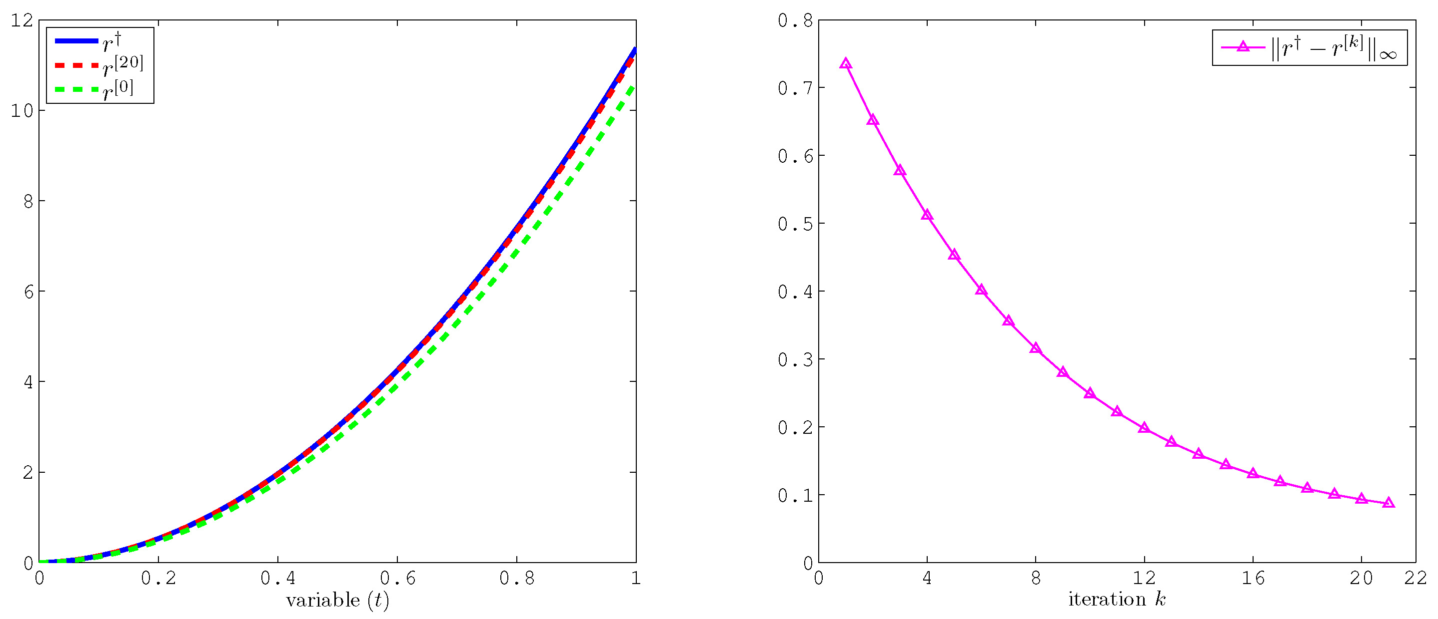
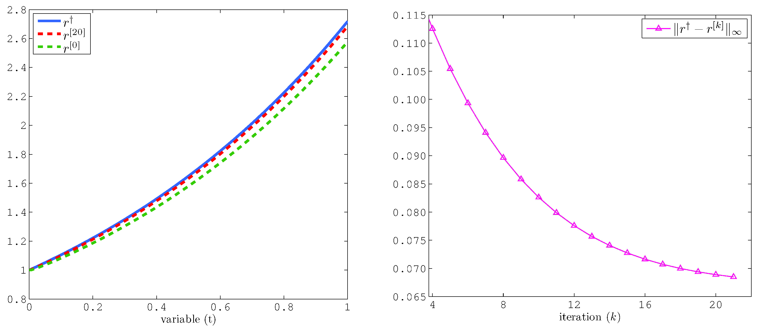
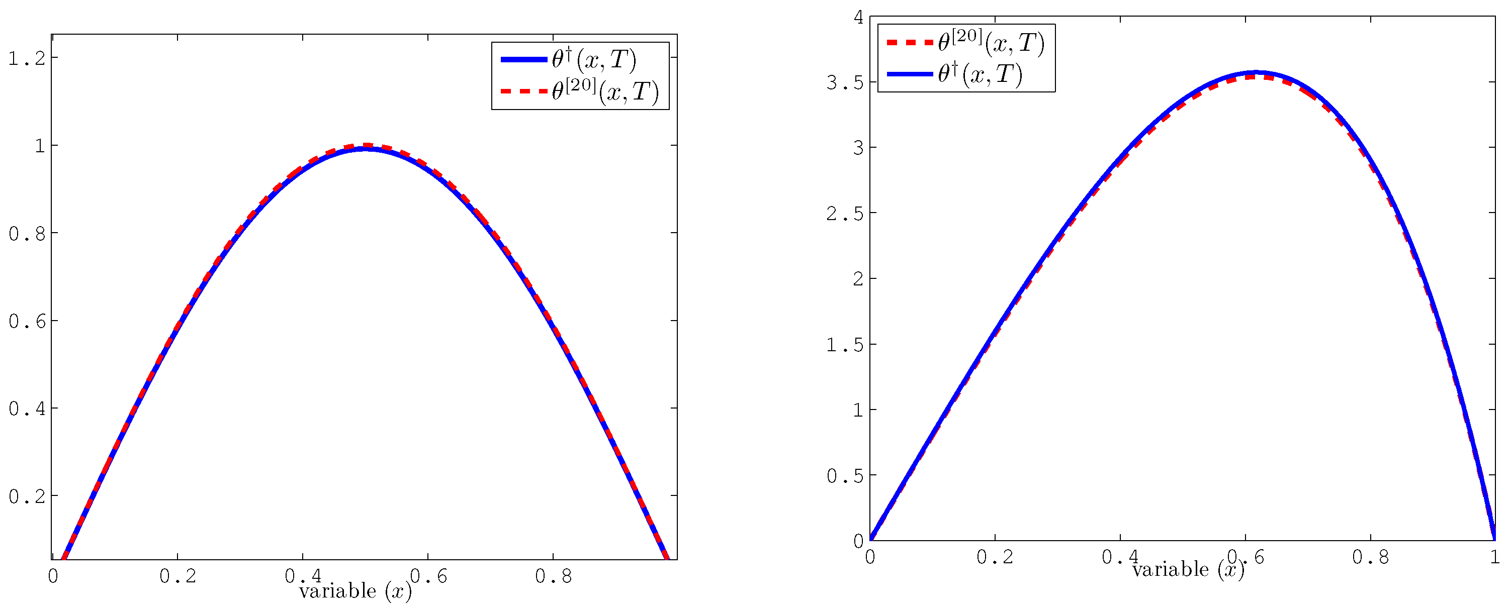
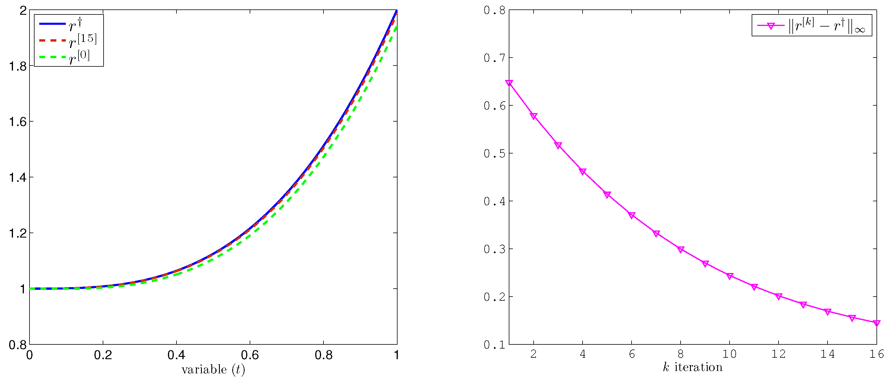
5. Numerical Reconstruction

In this section, our objective is to numerically reconstruct the missing unknown source term r ( t ) in Problems (1) and (2). Furthermore, we conduct a series of tests to evaluate the effectiveness of the proposed numerical method, designed to provide an approximate solution to the problem denoted as (6) and (7). The scheme itself can be derived directly from the discrete Problems (12) and (13). However, for more precise results, we deliberately adopt an L 1 -approximation scheme to discretize the Caputo fractional derivative.
Let { t n } 0 n N be a uniform partition of the time frame [ 0 , T ] with a time step τ = T / N . Based on a piecewise linear interpolation, the  L 1 -approximation scheme to the Caputo fractional derivative is given by
D t α θ ( t n + 1 ) D τ α θ n + 1 : = 1 Γ ( 1 α ) i = 0 n θ i + 1 θ i τ t i t i + 1 ( t n + 1 s ) α d s = 1 Γ ( 1 α ) i = 0 n θ n + 1 i θ n i τ t n i t n + 1 i s α d s = 1 Γ ( 2 α ) τ α i = 0 n b i α ( θ n + 1 i θ n i ) = 1 Γ ( 2 α ) τ α b 0 θ n + 1 + ( b 1 b 0 ) θ n + i = 1 n 1 ( b i α b i 1 α ) θ n i + b n α θ 0 ,
where b i α = ( i + 1 ) 1 α i 1 α . Notice that b 0 α = 1 ; it follows that
D τ θ n + 1 = 1 Γ ( 2 α ) τ α θ n + 1 + ( b 1 α 1 ) θ n + i = 1 n 1 ( b i α b i 1 α ) θ n i + b n α θ 0 = 1 Γ ( 2 α ) τ α θ n + 1 + H α n .
Divide the space domain [ 0 , 1 ] into subintervals M of uniformly equal length by points
ξ 0 = 0 < ξ 1 < ξ 2 < < ξ M = 1 , ξ i = i h x and h x = 1 / M .
Let P M ( Ω ) denote the space of all polynomials of degree at most M with respect to the variable x. The corresponding discrete space, denoted by V h , is then formally defined as
V h : = H a 1 ( K ) P M ( Ω ) .
The functions of V h , which are piecewise affine, can be represented using very simple basis functions, namely,
φ j ( x ) = x x i 1 h , x i 1 x x i , x i + 1 x h , x i x x i + 1 .
It is well known that any function φ h V h is uniquely defined by its value at the points ( ξ j ) 0 j M
φ h ( x ) = 0 = 1 M φ h ( ξ j ) φ j ( x ) , x [ 0 , 1 ] .
Now, we are in a position to define the linearized L 1 -Galerkin FEM, which reads as follows. Find θ h n V h ( n = 0 , , N ) satisfying for all φ h V h
D τ α θ h n , φ h + a x θ h n , x φ h = ( H α n , φ h ) + r n ( Π M p , φ ) + F ( θ h n 1 ) , φ h , n 0 , θ h 0 = Π M θ 0 , n = 0 ,
where Π M : L 2 ( Ω ) P M ( Ω ) is an interpolation operator. By noting (40), the above formulation can be rewritten as follows:
θ h n + 1 , φ h + α 0 a x θ h n , x φ h = ( H α n , φ h ) + α 0 r n ( Π M p , φ h ) + α 0 F ( θ h n 1 ) , φ h , n 0 , θ h 0 = Π M θ 0 , n = 0 ,
where α 0 = Γ ( 2 α ) t α . Now, taking φ h = φ j as a test function for j = 1 , , M 1 , we obtain
K + α 0 S Θ n + 1 = H n + α 0 r n + 1 P + α 0 F n , n 0 ,
where
Θ n = ( θ h n ( ξ 1 ) , θ h n ( ξ 2 ) , , θ h n ( ξ M 1 ) t ) , P = ( p 1 , p 2 , , p M 1 ) t , p j = ( Π M p , φ j ) , F n 1 = ( F 1 n 1 , F 2 n 1 , , F M 1 n 1 ) t , F j n 1 = ( F ( θ h n 1 ) , φ j ) , K = ( K j k ) 1 j , k M 1 , K j k = ( φ j , φ k ) , S = ( S j k ) 1 j , k M 1 , S j k = ( x φ j , x φ k ) , H n = ( H 1 n , H 2 n , , H M 1 n ) t , H k n = ( H n , φ k ) .
The values of r n for 0 n N are mainly resulted from Identities (13) and (20), namely,
r n = D t α E ( t n ) + ( x θ h n 1 , x ψ ) L 2 ( ω ) + ( F ( θ h n 1 ) , ψ ) L 2 ( ω ) ( p , ψ ) L 2 ( ω ) , n 1 , r 0 = ( x θ h 0 , x ψ ) L 2 ( ω ) + ( F ( θ h 0 ) , ψ ) L 2 ( ω ) ( p , ψ ) L 2 ( ω ) .
The numerical solution, hereinafter referred to as ( θ a p p , r a p p ) for clarity, obtained by solving System (41)–(43), can be considered an approximation for the solution of the underlying inverse problem. However, this numerical solution can be further refined by employing an iterative method to achieve more accurate results. The algorithm used can be described as follows.
For tests involving noisy data, we introduced artificial perturbations by adding a fixed-amplitude random component to the original data, namely,
E δ ( t ) = E ( t ) + δ × E ( t ) · rand ( 1 , 1 ) .
In order to demonstrate the effectiveness of the proposed algorithms, we now present some numerical examples in a one-dimensional setting.
Example 1. 
Consider the following problem:
D α θ ( x , t ) ( x β θ x ( x , t ) ) x = r ( t ) p ( x ) + F ( x , t ) , ( x , t ) ( 0 , 1 ) × ( 0 , 1 ) , θ ( x , 0 ) = x 3 2 sin ( π x ) , θ ( 0 , t ) = θ ( 1 , t ) = 0 ,
where
β = 1 2 , p ( x ) = x 2 sin ( π x ) , F ( x , t ) = 3 x sin ( π x ) + 9 π 2 x 3 / 2 cos ( π x ) π 2 x 5 / 2 sin ( π x ) ,
and the setting of the overdetermination Condition (2) is
ω = ( 0.4 , 0.5 ) , ψ ( x ) = ( x 0.4 ) ( x 0.5 ) , E ( t ) = 2 C ω Γ ( 3 α ) t 2 α , with C ω = ω x 2 s i n ( π x ) ψ ( x ) d x .
The exact solution is found as
θ ( x , t ) = ( t 2 + 1 ) x 2 sin ( π x ) , r ( t ) = 2 Γ ( 3 α ) t 2 α .
Figure 1 displays the profiles of reconstructed solutions r [ 0 ] , r [ 20 ] and the exact solution r . We note that, even without refinement, the reconstructed source term is qualitatively close to the exact one. However, after 20 iterations, the refined solution r [ 20 ] aligns perfectly with the exact profile. This fact is also confirmed by noticing the behavior of the error r r [ k ] acting as a function of k number of iterations (see Figure 1 (right)). The error decreases steadily, demonstrating that the iterative scheme effectively refines r a p p . Within about 20 to 25 iterations, the difference becomes negligible.
Figure 2 (left) further shows the reconstructed r [ k ] when the overspecified data E ( t ) are affected by different noise levels δ = 1 % , δ = 5 % , and δ = 10 % . In each case, the algorithm remains stable; while more noise degrades the recovered solution slightly, the shape and main features of the reconstructed solution remain recognizable. Likewise, Figure 2 (right) demonstrates that the iterative refinement is still effective under moderate noise levels, although more iterations are required for a larger noise level δ. While not explicitly mentioned, the iterative refinement in Algorithm 1 likely acts as implicit regularization, mitigating noise effects.
Algorithm 1  L 1 -Galerkin finite element method
1:
Initialization Solve (41)–(43) to obtain ( θ a p p , r a p p ) .
2:
Step 1: For k = 0 , set ( θ a p p , r a p p ) = ( θ [ 0 ] , r [ 0 ] ) .
3:
Step 2: For k 1 , set
4:
Solve (41) with r n = r n , [ k 1 ] to obtain ( θ [ k ] , r [ k ] ) .
5:
if  r [ k ] r [ k 1 ] < ϵ then
6:
    Take ( θ , r ) = ( θ [ k ] , r [ k ] ) as a refined solution.
7:
else
8:
    Update = k + 1 and go to Step 2.
9:
end if
Example 2. 
In this example, we perform our numerical tests in the presence of a nonlinear case. Let us consider the following problem:
D α θ ( x , t ) ( x β θ x ( x , t ) ) x = r ( t ) p ( x ) + g ( x , t ) + F ( u , x , t ) , ( x , t ) ( 0 , 1 ) × ( 0 , 1 ) , θ ( x , 0 ) = x 2 ( 1 x ) e x , θ ( 0 , t ) = θ ( 1 , t ) = 0 ,
where
β = 1 2 , p ( x ) = x 2 ( 1 x ) e x , F ( u , x , t ) = u 2 e ( x + t ) x + u x ,
and the setting of the overdetermination Condition (5) is
ω = ( 0.1 ; 0.8 ) , ψ ( x ) = ( x 0.1 ) ( x 0.8 ) , E ( t ) = C ω e t , with C ω = ω x 2 ( 1 x ) e x ψ ( x ) d x .
The exact solution is found as
θ ( x , t ) = x 2 ( 1 x ) e x e t , r ( t ) = t E 1 , 3 2 ( t ) .
In this example, the nonlinear term F ( θ ) introduces additional complexity. Despite this, the numerical results, illustrated by Figure 3, confirm that introducing nonlinearity into the PDE does not substantially degrade performance.
As shown in Figure 3 (left), even with an initial reconstructed solution r [ 0 ] far from the exact solution, the subsequent iterations rapidly reduce the discrepancy. Figure 3 (right) confirms that the error r r [ k ] decreases steadily as the number of iterations k increases, and then its value becomes constant in fewer than 20 iterations. The obtained results confirm the method converges within a few iterations, even with the nonlinear forcing term, and the reconstructed solutions θ [ k ] and r [ k ] (Figure 4) match the exact solutions closely.
Figure 5 (left) shows the reconstructions for different noise levels δ = 1 , 5 , 10 % . As in Example 1, the iterative scheme remains robust, so that the reconstructed source term r [ k ] remains close to its exact counterpart, with only a small degradation in the presence of higher noise. Figure 5 (right) shows that even for δ = 10 % , the method converges, though it may require more iterations.
Overall, Example 2 shows greater sensitivity to noise compared to Example 1; this is completely logical as the nonlinear term F ( θ ) propagates errors. Nevertheless, the reconstructed r [ k ] remains within acceptable bounds of the exact solution.
Example 3. 
In this example, we aim to test the validity of the designed numerical algorithm for solving two-dimensional problems. Let us consider the following problem:
D t α θ d i v ( A ( x , y ) θ ) = r ( t ) p ( x , y ) + F ( x , y , t ) , ( x , y , t ) Ω × ( 0 , T ) , θ ( x , y , 0 ) = θ 0 ( x , y ) , ( x , y ) Ω : = ( 0 , 1 ) 2 , θ ( x , y , t ) = 0 , ( x , y , t ) Ω × ( 0 , T ) ,
and the over-determination data are given as
E ( t ) = C ω ( t 3 + 1 ) = ω θ ( x , y , t ) ψ ( x , t ) d x d y ,
where
ψ ( x , y ) = ( x 2 3 10 x + 1 50 ) ( y 2 3 10 y + 1 50 ) , ( x , y ) ω : = ( 0.1 ; 0.2 ) × ( 0.1 ; 0.2 ) .
The exact solution is given explicitly as
u ( x , y , t ) = x 2 y 2 ( x 1 ) ( y 1 ) × ( t 3 + 1 ) , r ( t ) = 6 Γ ( 4 α ) t 3 α , ( x , y ) Ω , t [ 0 , T ] .
Figure 6 and Figure 7 summarize the numerical reconstruction performance. On the left of Figure 6, the profiles of the exact source term r , the initial approximation r [ 0 ] , and the refined solution r [ 20 ] are illustrated, while the right figure displays the convergence behavior via the error r r [ k ] against the number of iterations k. These results are analogous to those observed in the one-dimensional case, confirming that the reconstruction method maintains similar accuracy and convergence.
On the left of Figure 6, we compare the exact source term r , the initial reconstruction r [ 0 ] , and the refined solution r [ 15 ] , showing alignment after 15 iterations. The right plot illustrates the error r r [ k ] decreasing steadily with iterations. The left plot of Figure 7 displays the reconstructed r [ k ] under different noise levels ( δ = 1 % , 5 % , 10 % ), while the right one shows error behavior as a function of the number of iterations, even for noisy data.
The numerical results for the two-dimensional settings problem mirror the one-dimensional cases (Examples 1 and 3); iterative refinement effectively reduces errors, and the method remains stable under moderate noise. Despite the added complexity of higher dimensionality, the algorithm retains its convergence properties and robustness, consistent with the one-dimensional framework.

6. Conclusions

In this study, we address the inverse problem of identifying a time-dependent source term in a time-fractional degenerate semi-linear parabolic equation by using an integral measurement on a subdomain. By employing the Rothe method, we rigorously established the existence and uniqueness of a weak solution under reasonable conditions.A priori estimates derived for discretized solutions facilitated the convergence of Rothe functions to the desired solution, ensuring the well posedness of the inverse problem. It appears that the Rothe method, considered a constructive approach, has a numerical extension, which we utilized to design an effective algorithm for the numerical reconstruction of the unknown source term. The numerical framework, combining an L 1 -Galerkin finite element scheme with an iterative refinement algorithm, demonstrated the robust reconstruction of the source term even in the presence of nonlinearities and noise-overdetermined data. Numerical experiments confirmed the proposed method’s stability and accuracy, highlighting its resilience to moderate noise levels and its capacity to handle nonlinear forcing terms effectively.
In future work, we aim mainly to extend the methodology presented in the current work to multi-dimensional domains or systems of coupled fractional degenerate parabolic equations that could address more complex physical phenomena, such as multi-component diffusion-reaction processes.

Author Contributions

Conceptualization, M.N., C.A., O.M.A. and H.O.S.; formal analysis, M.N., C.A., O.M.A. and H.O.S.; funding acquisition, M.N., C.A. and H.O.S.; methodology, C.A. and O.M.A.; software, M.N. and C.A.; supervision, C.A. and H.O.S.; visualization, H.O.S.; writing—original draft, M.N., C.A., O.M.A. and H.O.S.; writing—review and editing, C.A. and O.M.A. All authors have read and agreed to the published version of this manuscript.

Funding

This research work was funded by Umm Al-Qura University, Saudi Arabia, under grant number: 25UQU4330056GSSR01.

Data Availability Statement

The original contributions presented in this study are included in the article. Further inquiries can be directed to the corresponding author.

Conflicts of Interest

The authors declares no conflict of interest.

References

  1. Buchot, J.-M.; Raymond, J.-P. A linearized model for boundary layer equations. In Optimal Control of Complex Structures: International Conference in Oberwolfach, 4–10 June 2000; Springer: Berlin/Heidelberg, Germany, 2001; pp. 31–42. [Google Scholar]
  2. Cannarsa, P.; Fragnelli, G.; Rocchetti, D. Controllability results for a class of one-dimensional degenerate parabolic problems in nondivergence form. J. Evol. Equ. 2008, 8, 583–616. [Google Scholar] [CrossRef]
  3. Martinez, P.; Raymond, J.-P.; Vancostenoble, J. Regional null controllability for a linearized Crocco-type equation. SIAM J. Control Optim. 2003, 42, 709–728. [Google Scholar] [CrossRef]
  4. Bertero, M.; Boccacci, P.; De Mol, C. Introduction to Inverse Problems in Imaging, 2nd ed.; CRC Press: Boca Raton, FL, USA, 2021. [Google Scholar]
  5. Mazaheri, M.; Mohammad Vali Samani, J.; Samani, H.M.V. Mathematical model for pollution source identification in rivers. Environ. Forensics 2015, 16, 310–321. [Google Scholar] [CrossRef]
  6. Zaporozhets, A.O.; Khaidurov, V.V. Mathematical models of inverse problems for finding the main characteristics of air pollution sources. Water Air Soil Pollut. 2020, 231, 563. [Google Scholar] [CrossRef]
  7. Tanaka, M.; Dulikravich, G.S. (Eds.) Inverse Problems in Engineering Mechanics; Elsevier: Amsterdam, The Netherlands, 1998. [Google Scholar]
  8. Oldenburg, D.W.; Pratt, D.A. Geophysical inversion for mineral exploration: A decade of progress in theory and practice. Proc. Explor. 2007, 7, 61–95. [Google Scholar]
  9. Persova, M.G.; Soloveichik, Y.G.; Vagin, D.V.; Grif, A.M.; Kiselev, D.S.; Patrushev, I.I.; Ganiev, B.G. The design of high-viscosity oil reservoir model based on the inverse problem solution. J. Pet. Sci. Eng. 2021, 199, 108245. [Google Scholar] [CrossRef]
  10. Metzler, R.; Klafter, J. The random walk’s guide to anomalous diffusion: A fractional dynamics approach. Phys. Rep. 2000, 339, 1–77. [Google Scholar] [CrossRef]
  11. Müller, S.; Kästner, M.; Brummund, J.; Ulbricht, V. A nonlinear fractional viscoelastic material model for polymers. Comput. Mater. Sci. 2011, 50, 2938–2949. [Google Scholar] [CrossRef]
  12. Oliveira, F.A.; Ferreira, R.M.; Lapas, L.C.; Vainstein, M.H. Anomalous diffusion: A basic mechanism for the evolution of inhomogeneous systems. Front. Phys. 2019, 7, 18. [Google Scholar] [CrossRef]
  13. Benabbes, F.; Boussetila, N.; Lakhdari, A. Two regularization methods for a class of inverse fractional pseudo-parabolic equations with involution perturbation. Fract. Differ. Calc. 2024, 14, 39–59. [Google Scholar] [CrossRef]
  14. Deng, Z.; Yang, L. An inverse problem of identifying the radiative coefficient in a degenerate parabolic equation. Chin. Ann. Math. 2014, 35, 355–382. [Google Scholar] [CrossRef]
  15. Durdiev, D.K.; Sultanov, M.A.; Rahmonov, A.A.; Nurlanuly, Y. Inverse Problems for a Time-Fractional Diffusion Equation with Unknown Right-Hand Side. Progr. Fract. Differ. Appl. 2023, 9, 639–653. [Google Scholar]
  16. Hasanoğlu, A.H.; Romanov, V.G. Introduction to Inverse Problems for Differential Equations; Springer: Cham, Switzerland, 2021. [Google Scholar]
  17. Huzyk, N.M.; Pukach, P.Y.; Vovk, M.I. Coefficient inverse problem for the strongly degenerate parabolic equation. Carpathian J. Math. 2023, 15, 52–65. [Google Scholar]
  18. Isakov, V. Inverse Problems for Partial Differential Equations; Springer: New York, NY, USA, 2006; Volume 127. [Google Scholar]
  19. Jin, B.; Rundell, W. An inverse problem for a one-dimensional time-fractional diffusion problem. Inverse Probl. 2012, 28, 075010. [Google Scholar]
  20. Kaltenbacher, B.; Rundell, W. Inverse Problems for Fractional Partial Differential Equations; American Mathematical Society: Providence, RI, USA, 2023; Volume 230. [Google Scholar]
  21. Kirane, M.; Lopushansky, A.; Lopushanska, H. Inverse problem for a time-fractional differential equation with a time-and space-integral conditions. Math. Methods Appl. Sci. 2023, 46, 16381–16393. [Google Scholar] [CrossRef]
  22. Grimmonprez, M.; Slodička, M. Reconstruction of an unknown source parameter in a semilinear parabolic problem. J. Comput. Appl. Math. 2015, 289, 331–345. [Google Scholar] [CrossRef]
  23. Van Bockstal, K.; De Staelen, R.H.; Slodička, M. Identification of a memory kernel in a semilinear integrodifferential parabolic problem with applications in heat conduction with memory. J. Comput. Appl. Math. 2015, 289, 196–207. [Google Scholar]
  24. Bekakra, Y.; Bouziani, A. Rothe Time-discretization Method for Caputo Fractional Parabolic Equation. Lobachevskii J. Math. 2024, 45, 3873–3883. [Google Scholar] [CrossRef]
  25. Chattouh, A.; Saoudi, K.; Nouar, M. Rothe–Legendre pseudospectral method for a semilinear pseudoparabolic equation with nonclassical boundary condition. Nonlinear Anal. Model. Control 2022, 27, 38–53. [Google Scholar] [CrossRef]
  26. Slodička, M.; Šišková, K. An inverse source problem in a semilinear time-fractional diffusion equation. Comput. Math. Appl. 2016, 72, 1655–1669. [Google Scholar] [CrossRef]
  27. Wei, T.; Li, X.L.; Li, Y.S. An inverse time-dependent source problem for a time-fractional diffusion equation. Inverse Probl. 2016, 32, 085003. [Google Scholar] [CrossRef]
  28. Ruan, Z.; Wang, Z. Identification of a time-dependent source term for a time fractional diffusion problem. Appl. Anal. 2017, 96, 1638–1655. [Google Scholar] [CrossRef]
  29. Liu, S.; Feng, L.; Liu, C. A Fractional Tikhonov Regularization Method for Identifying a Time-Independent Source in the Fractional Rayleigh–Stokes Equation. Fractal Fract. 2024, 8, 601. [Google Scholar] [CrossRef]
  30. Wei, T.; Wang, J. A modified quasi-boundary value method for an inverse source problem of the time-fractional diffusion equation. Appl. Numer. Math. 2014, 78, 95–111. [Google Scholar] [CrossRef]
  31. Ruan, Z.; Wan, G.; Zhang, W. Reconstruction of a space-dependent source term for a time fractional diffusion equation by a modified quasi-boundary value regularization method. Taiwan. J. Math. 2024, 1, 1–23. [Google Scholar] [CrossRef]
  32. Li, Z.; Deng, Z. A total variation regularization method for an inverse problem of recovering an unknown diffusion coefficient in a parabolic equation. Inverse Probl. Sci. Eng. 2020, 28, 1453–1473. [Google Scholar] [CrossRef]
  33. Klibanov, M.V.; Li, J.; Zhang, W. Convexification for an inverse parabolic problem. Inverse Probl. Sci. Eng. 2020, 28, 605–635. [Google Scholar] [CrossRef]
  34. Lv, X.; Feng, X. Identifying a Space-Dependent Source Term and the Initial Value in a Time Fractional Diffusion-Wave Equation. Mathematics 2023, 11, 1521. [Google Scholar] [CrossRef]
  35. Sidi, H.O.; Hendy, A.S.; Babatin, M.M.; Qiao, L.; Zaky, M.A. An inverse problem of Robin coefficient identification in parabolic equations with interior degeneracy from terminal observation data. Appl. Numer. Math. 2025, 212, 242–253. [Google Scholar] [CrossRef]
  36. Nouar, M.; Chattouh, A. On the source identification problem for a degenerate time-fractional diffusion equation. J. Math. Anal. 2024, 15, 84–98. [Google Scholar] [CrossRef]
  37. Chen, Y.-G.; Yang, F.; Tian, F. The Landweber Iterative Regularization Method for Identifying the Unknown Source of Caputo-Fabrizio Time Fractional Diffusion Equation on Spherically Symmetric Domain. Symmetry 2023, 15, 1468. [Google Scholar] [CrossRef]
  38. Jiang, D.; Feng, H.; Zou, J. Quadratic convergence of Levenberg-Marquardt method for elliptic and parabolic inverse robin problems. ESAIM Math. Model. Numer. Anal. 2018, 52, 1085–1107. [Google Scholar] [CrossRef]
  39. Fragnelli, G.; Goldstein, G.R.; Goldstein, J.A.; Romanelli, S. Generators with interior degeneracy on spaces of L2 type. Electron. J. Differ. Equ. 2012, 2012, 1–30. [Google Scholar]
  40. Maes, F.; Van Bockstal, K. Existence and uniqueness of a weak solution to fractional single-phase-lag heat equation. Fract. Calc. Appl. Anal. 2023, 26, 1663–1690. [Google Scholar] [CrossRef]
  41. Alsaedi, A.; Ahmad, B.; Kirane, M. A survey of useful inequalities in fractional calculus. Fract. Calc. Appl. Anal. 2017, 20, 574–594. [Google Scholar] [CrossRef]
  42. Kačur, J. Method of Rothe in Evolution Equations. In Equadiff 6; Springer: Berlin/Heidelberg, Germany, 1985. [Google Scholar]
Figure 1. Numerical results for Example (1). (Left) profiles of exact source term r , reconstructed source term r [ 0 ] , and refined solution r [ 20 ] . (Right) the error r r [ k ] versus k.
Mathematics 13 01486 g001
Figure 2. Numerical results for Example (1). (Left) reconstructed source term with different noise levels. (Right) the error r r [ k ] versus k.
Mathematics 13 01486 g002
Figure 3. Numerical results for Example 2. (Left) profiles of exact source term r , reconstructed source term r [ 0 ] , and refined solution r [ 22 ] . (Right) the error r r [ k ] versus k.
Mathematics 13 01486 g003
Figure 4. (Left) reconstruction of θ ( x , T ) in Example 1. (Right) reconstruction of θ ( x , T ) in Example 2.
Mathematics 13 01486 g004
Figure 5. Numerical results for Example (2). (Left) reconstructed source term with different noise levels. (Right) the error r r [ k ] versus k.
Mathematics 13 01486 g005
Figure 6. Numerical results for Example 3. (Left) profiles of exact source term r , reconstructed source term r [ 0 ] , and refined solution r [ 15 ] . (Right) the error r r [ k ] versus k.
Mathematics 13 01486 g006
Figure 7. Numerical results for Example 3. (Left) reconstructed source term with different noise levels. (Right) the error r r [ k ] versus k.
Mathematics 13 01486 g007
Disclaimer/Publisher’s Note: The statements, opinions and data contained in all publications are solely those of the individual author(s) and contributor(s) and not of MDPI and/or the editor(s). MDPI and/or the editor(s) disclaim responsibility for any injury to people or property resulting from any ideas, methods, instructions or products referred to in the content.

