Advances in Multi-Source Navigation Data Fusion Processing Methods

Abstract

In recent years, the field of multi-source navigation data fusion has witnessed substantial advancements, propelled by the rapid development of multi-sensor technologies, Artificial Intelligence (AI) algorithms and enhanced computational capabilities. On one hand, fusion methods based on filtering theory, such as Kalman Filtering (KF), Particle Filtering (PF), and Federated Filtering (FF), have been continuously optimized, enabling effective handling of non-linear and non-Gaussian noise issues. On the other hand, the introduction of AI technologies like deep learning and reinforcement learning has provided new solutions for multi-source data fusion, particularly enhancing adaptive capabilities in complex and dynamic environments. Additionally, methods based on Factor Graph Optimization (FGO) have also demonstrated advantages in multi-source data fusion, offering better handling of global consistency problems. In the future, with the widespread adoption of technologies such as 5G, the Internet of Things, and edge computing, multi-source navigation data fusion is expected to evolve towards real-time processing, intelligence, and distributed systems. So far, fusion methods mainly include optimal estimation methods, filtering methods, uncertain reasoning methods, Multiple Model Estimation (MME), AI, and so on. To analyze the performance of these methods and provide a reliable theoretical reference and basis for the design and development of a multi-source data fusion system, this paper summarizes the characteristics of these fusion methods and their corresponding application scenarios. These results can provide references for theoretical research, system development, and application in the fields of autonomous driving, unmanned vehicle navigation, and intelligent navigation.

1. Introduction

Individually, Global Navigation Satellite Systems (GNSS), Inertial Navigation Systems (INS), Ultra-Wideband (UWB) technology, Bluetooth, Wireless Local Area Networks (WLAN), visual sensors, Pseudolites (PL), and various other sensors struggle to meet demanding navigation performance requirements. GNSS, for instance, as a non-autonomous navigation system, is particularly limited in specific complex environments such as urban canyons and tunnels, where its signals are highly susceptible to blockage, interference, and shielding. To significantly enhance the overall performance of navigation systems, integrated navigation technology emerges as an effective solution. This technology entails the collaborative use of two or more distinct types of navigation systems to measure and calculate the same navigation information, thereby generating quantitative measurements. These measurements are subsequently utilized to compute and correct the errors inherent in each navigation system. By leveraging a diverse array of technical means and methods, this approach ensures high accuracy and reliability of navigation and positioning services across a wide range of scenarios. These scenarios encompass seamless indoor and outdoor positioning, environments with electromagnetic interference, as well as underwater and underground environments. Therefore, multi-source data fusion positioning, which is founded on the collaboration of multiple technology sources and adheres to specific optimization criteria, becomes the linchpin for achieving optimal fusion positioning. The fusion method not only serves as the prerequisite and foundation for all-source navigation but also acts as the key and core of integrated navigation systems.

The concept of data fusion was first introduced by the renowned American systems scientist Bar-Shalom in his seminal article titled ‘Extension of the Probabilistic Data Association Filter in Multi-Target Tracking’. In this pioneering work, he proposed the probabilistic data interconnection filter, which has since become a hallmark of multi-source information fusion technology. Over the years, multi-source data fusion methods have evolved and diversified. Currently, the primary approaches employed in this field include the switching method, the average weighted fusion method, and the adaptive weighted fusion method. Each of these methods offers unique advantages and is tailored to address specific challenges in data fusion, thereby enhancing the overall effectiveness and reliability of integrated navigation and positioning systems.

Based on the performance of different positioning sources, the optimal single positioning source is selected as the positioning means [1]. However, ignoring other positioning sources is a waste and not the best choice. The average weighted fusion method does not take into account the different performances of different positioning sources but assigns the same weight to all positioning sources for fusion localization [2], which cannot achieve the optimal fusion effect. The adaptive weighted fusion method assigns different weights according to the characteristics of different fusion sources to achieve the best fusion positioning [3]. The algorithms corresponding to these three methods mainly include optimal estimation algorithms, weighted fusion algorithms or adaptive weighted fusion algorithms [4,5,6], Bayesian filters (BF), variable-decibel Bayesian adaptive estimation [7,8], Particle Filter (PF), Statistical decision theory [9], evidence theory [10], fuzzy logic [11], etc. However, these algorithms all have specific preconditions and application scenarios, and it is necessary to establish a mathematical model between the observation information of the navigation source and the system state parameters.

In the field of dynamic positioning such as autonomous driving and vehicle navigation, the Kalman Filter (KF) has been widely used due to the introduction of physical motion models. However, KF is primarily designed for linear systems. For nonlinear systems, such as inertial navigation, the Extended KF (EKF) is suitable for weakly nonlinear objects because higher-order terms above the second order are discarded in the linearization process. To address the issue that the batch processing of the EKF random model requires storing a large amount of data, a recursive method for the random model has been proposed [12], and time-domain non-local filtering data fusion algorithms have also been included [13]. The Unscented KF (UKF) retains the accuracy achieved by the third-order term of the Taylor series, making it suitable for nonlinear object estimation, although it involves relatively high computational demands. When both the system state and measurement noise are nonlinear, the PF can be used for nonlinear systems and systems with uncertain error models. However, the PF requires a probability density that closely approximates the real density. Otherwise, the filtering effect may be poor or even divergent. To address this, the Unscented Kalman Particle Filter (UPF) algorithm has been developed [14]. However, both the PF and UPF methods face the issue of rapidly increasing computational load as the number of particles grows.

With the increasing demand from users for more comprehensive and intelligent navigation and positioning performance, filtering methods such as Factor Graphs (FG) and neural networks have been introduced. For example, FG algorithms have been extensively applied in single GNSS positioning, GNSS/INS integrated positioning, ambiguity resolution, and robust estimation [15,16,17,18]. To enhance positioning accuracy in urban environments, FG algorithms have been optimized and improved [19,20]. These studies have demonstrated that under certain conditions, FG algorithms exhibit higher computational accuracy and robustness compared to EKF. In 1965, Magill proposed the Multi-Model Estimation (MME) method [21], which enhances the adaptability of system models to real systems and changes in external environments under complex conditions, thereby improving the accuracy and stability of filtering estimates. The design of the model set, the selection of filters, estimation fusion, and the reset of filter inputs are all very important aspects. To enhance the high fault-tolerance capability of integrated navigation systems, Carlson introduced the Federated Filtering (FF) theory in 1988 [22]. This theory has been applied in indoor navigation, robotic navigation, and vision–language tasks. Existing Artificial Intelligence (AI) algorithms mainly include fuzzy control adaptive algorithms and neural network adaptive algorithms [23,24]. For example, to address the impact of random disturbances on systems in underwater environments, RBF neural network-assisted FF has been employed for information fusion [25]. By establishing a black box model with sufficiently accurate samples through offline training, the positioning accuracy and adaptability of the algorithm have been improved. To tackle the issues of high cost and susceptibility to weather conditions in existing high-precision satellite navigation for agricultural machinery, Yu et al. (2021) proposed a multi-sensor fusion automatic navigation method for farmland based on D-S-CNN [26]. However, these AI algorithms require extensive training data, comprehensive pre-training of the system, and significant computational resources, and often struggle to ensure real-time performance, typically being used for post-processing.

Recently, scholars from various countries have conducted extensive research on integrated navigation systems. For instance, researchers from Linköping University in Sweden proposed a combined navigation system that integrates GPS, INS, and visible light vision assistance [27]. This system utilizes the vision system and INS for positioning when GPS fails. Locata Corporation in Australia has integrated the Locata system with GPS, INS, vision systems, and Simultaneous Localization and Mapping (SLAM), achieving high-precision applications of the Locata system in both indoor and outdoor environments [28]. A communication and navigation fusion system has been applied for seamless positioning across wide-area indoor and outdoor spaces [29]. A multi-frequency ground-penetrating radar data fusion system is used for working antennas in different frequency ranges [30], while multi-sensor data fusion is employed for analyzing airspeed measurement fault detection in drones [3]. Additionally, an indoor mobile robot based on dead reckoning data fusion and fast response code detection [31], and an IoT-based multi-sensor fusion strategy for analyzing occupancy sensing systems in smart buildings have been developed [32]. Systems that integrate vision, inertial navigation, and asynchronous optical tracking with Inertial Measurement Units (IMU) have also been implemented. Furthermore, several research teams have successfully developed open-source integrated navigation systems for use by academic or industrial technical personnel [33,34,35].

Although the aforementioned studies include extensive research and testing on multi-source data fusion methods, fusion systems, and their applications, the theories and models of these methods have their specific applicable scenarios and conditions. Therefore, this paper summarizes the fundamental principles and mathematical models of multi-source data fusion methods, analyzes the advantages and disadvantages of different fusion approaches, and provides theoretical support and reference for the design, development, and application of fusion systems.

2. Multi-Source Navigation Data Fusion Processing Method

Fusion methods are primarily categorized into optimal estimation methods, filtering methods, MME, FG, FF, and other fusion approaches. The following sections will focus on elaborating the basic principles of these methods, their corresponding algorithmic models, and applicable scenarios.

2.1. Optimal Estimation Method

We estimate the parameter by utilizing randomly distributed observation vectors. Specifically, we seek a mapping function to compute the estimated value. In this context, the system state is characterized by the vector $x$, while the measurements from various navigation sources are denoted by $y$. The observation equations, which can be either nonlinear or linear, are formulated as follows:

$$y=Ax+\epsilon$$

(1)

where $A$ is the observation matrix. $\epsilon$ includes the error term caused by random observation noise and linearization. The state of the system can be estimated by observation, and the estimated result is a vector $\widehat{x}$.

By employing different estimation criteria to address the problem of estimating unknown parameters, various estimation methods can be derived. Based on Equation (1) and the optimization of the criterion function, methods such as Least Squares Estimation (LSE), Minimum Variance Estimation (MVE), Maximum Likelihood Estimation (MLE), and Maximum A Posteriori Estimation (MAPE) can be formulated.

2.1.1. General LSE and Weighted LSE (WLSE)

The LSE is a parameter estimation algorithm proposed by the German mathematician Carl Friedrich Gauss in 1795, initially developed to determine planetary orbits [36]. Regardless of whether the variable $x$ in the linear model (2) possesses prior statistical information or the random distribution followed by $y$, the LSE criterion employs a quadratic minimum.

$$J\left(\widehat{x}\right)={\left(y-Ax\right)}^{\mathrm{{\rm T}}}W\left(y-Ax\right)=\min$$

(2)

where $W$ is the appropriate positive definite weighted matrix, the above formula is the general LSE criterion when $W=I$. Then, the estimation error and its variance are as follows:

$$\left\{\begin{array}{l}{\widehat{x}}_{LS}={\left(A^{\mathrm{{\rm T}}}WA\right)}^{-1}{A}^{\mathrm{{\rm T}}}Wy\\ {\Sigma }_{\delta {\widehat{x}}_{LS}}={\left(A^{\mathrm{{\rm T}}}WA\right)}^{-1}{A}^{\mathrm{{\rm T}}}W{\Sigma }_{\epsilon }WA{\left(A^{\mathrm{{\rm T}}}WA\right)}^{-1}\end{array}\right.$$

(3)

It is easy to prove that when $W={\Sigma }_{\epsilon }^{-1}$, LSE has a minimum variance [36,37].

The most significant feature of this method lies in its algorithmic simplicity and independence from statistical information related to estimators and measurements. Previous researchers have implemented this algorithm in multi-source data fusion processing [38,39]. However, the LSE exclusively utilizes measurement information for current state estimation, a characteristic that paradoxically constrains its applicability. Furthermore, while the LSE optimality criterion guarantees the minimization of the total mean squared error in measurement estimates, it fails to ensure optimal estimation error for the estimator itself, consequently leading to suboptimal estimation accuracy.

2.1.2. MLE

Let the conditional probability density of $y$ with respect to $x$ be $f\left(y/x\right)$ and the MLE criterion be the following:

$${\left.f\left(y/x\right)\right|}_{x={\widehat{x}}_{ML}}=\max$$

(4)

This means that $y$ has its maximum value at ${\left.f\left(y/x\right)\right|}_{x={\widehat{x}}_{ML}}=\max$, which is equivalent to the following:

$$\partial f\left(y/x\right)/\mathsf{\partial }x{|}_{x={\widehat{x}}_{ML}}=0$$

(5)

Obviously, the solution of Equation (5) is related to $f\left(y/x\right)$. Different conditional probability density functions lead to different valuation formulas, therefore a universal formula cannot be derived. When $f\left(y/x\right)$ follows a normal distribution, for example:

$$f\left(y/x\right)={\displaystyle \frac{1}{{\left(2\pi \right)}^{n/2}{\left|{\Sigma }_{y/x}\right|}^{1/2}}}\exp \left\{-{\displaystyle \frac{{\left(y-E\left(y/x\right)\right)}^{\mathrm{{\rm T}}}{\Sigma }_{y/x}^{-1}\left(y-E\left(y/x\right)\right)}{2}}\right\}$$

(6)

The expectation and variance formulas under the normal distribution condition are as follows: [36,37]

$$\left\{\begin{array}{l}E\left(y/x\right)=E\left(y\right)+{\Sigma }_{yx}{\Sigma }_x^{-1}\left(x-E\left(x\right)\right)\\ {\Sigma }_{y/x}={\Sigma }_y-{\Sigma }_{yx}{\Sigma }_x^{-1}{\Sigma }_{xy}\end{array}\right.$$

(7)

From the above derivation, it can be concluded that MLE does not require prior distribution information about $x$. However, when its prior distribution information is known, $f\left(y/x\right)$ should be derived strictly based on Equation (5).

2.1.3. MAPE

The estimation ${\widehat{x}}_{MA}$ of MAPE makes $f\left(x/y\right)$ reach the maximum value under the condition $\widehat{x}={\widehat{x}}_{MA}$. The equivalent MAPE criteria are as follows after similar derivation [37]:

$${\left.f\left(x/y\right)\right|}_{\widehat{x}={\widehat{x}}_{MA}}=\max$$

(8)

According to the conditional probability formula, it is easy to prove that (8) is equivalent to the following:

$${\left.f\left(x/y\right)\right|}_{\widehat{x}={\widehat{x}}_{MA}}=f\left(x/y\right)/f_2\left(y\right){|}_{\widehat{x}={\widehat{x}}_{MA}}=\max \iff f\left(x,y\right){|}_{\widehat{x}={\widehat{x}}_{MA}}=\max$$

(9)

That is, the MAPE employs the joint probability density function of the parameters and the observed data as its maximization criterion.

When both y and $x$ are normally distributed, the conditional probability density function is as follows:

$$f\left(x/y\right)={\displaystyle \frac{1}{{\left(2\pi \right)}^{t/2}\left|{\Sigma }_{x/y}\right|}}\exp \left\{-{\displaystyle \frac{{\left(x-E\left(x/y\right)\right)}^{\mathrm{{\rm T}}}{\Sigma }_{x/y}^{-1}\left(x-E\left(x/y\right)\right)}{2}}\right\}$$

(10)

Differentiate Equation (10) and set the derivative to zero to obtain the variance and estimation error of the MAPE:

$$\left\{\begin{array}{l}{\widehat{x}}_{MA}=E\left(x/y\right)\\ {\Sigma }_{\delta {\widehat{x}}_{MA}}={\Sigma }_{x/y}\end{array}\right.$$

(11)

When x is uncorrelated with y, the estimated result is equal to the prior information of the parameter.

Compared with MLE, MAPE places greater emphasis on the prior information of parameters. Therefore, MAPE becomes meaningless when parameters are non-random quantities. In practice, MAPE can be understood as a modification of parameters through observational data, where the extent of this modification is determined by the variance of the observations and their correlation with the parameters.

2.1.4. MVE

The MVE is an optimization criterion that minimizes the variance of the estimation error to estimate ${\widehat{x}}_{MV}$.

$$J\left(\widehat{x}\right)={\left.E\left({\left(x-{\widehat{x}}_{MV}\right)}^{\mathrm{{\rm T}}}\left(x-{\widehat{x}}_{MV}\right)\right)\right|}_{\widehat{x}={\widehat{x}}_{MV}}={\displaystyle {\int }_{-\infty }^{\infty }{\displaystyle {\int }_{-\infty }^{\infty }{\left(x-{\widehat{x}}_{MV}\right)}^{\mathrm{{\rm T}}}\left(x-{\widehat{x}}_{MV}\right)}}f\left(x,y\right)dxdy=\min$$

(12)

According to the conditional and edge probability density functions, Equation (12) is equivalent to the following:

$$h\left({\widehat{x}}_{MV}\right)={\displaystyle {\int }_{-\infty }^{\infty }{\left(x-{\widehat{x}}_{MV}\right)}^{\mathrm{{\rm T}}}\left(x-{\widehat{x}}_{MV}\right)}dx=\min$$

(13)

The MVE and its estimation error are as follows:

$$\left\{\begin{array}{l}{\widehat{x}}_{MV}=E\left(x/y\right)\\ {\Sigma }_{\delta {\widehat{x}}_{MV}}={\displaystyle {\int }_{-\infty }^{\infty }{\Sigma }_{x/y}}{f}_2\left(y\right)dy\end{array}\right.$$

(14)

where $f_2\left(y\right)$ is the edge probability density function of the observation. When both the x and the y are normally distributed, the MVE is completely equivalent to the MAPE.

2.1.5. LMVE

MLE, MAPE, and MVE all necessitate the joint probability density or conditional probability density function of $\mathit{y}$ and $\mathit{x}$. Their estimation formulas hinge on distributional information and do not necessarily manifest as linear combinations of the observed values. In contrast, the LSE dispenses with the need for distributional information of the parameters and observed values. Instead, it formulates parameter estimation as a linear combination of the observed values, thus qualifying as a linear estimation technique. As the name implies, the LMVE is also a linear estimation method. It does not require any specific distributional information of the observed values and parameters, relying only on their statistical properties.

Let LMVE be estimated as the following:

$${\widehat{x}}_{LMV}=\alpha +\beta y$$

(15)

where $\alpha$ is a constant vector and $\beta$ is a constant matrix, then the estimation error and its variance are as follows:

$$\left\{\begin{array}{l}\delta {\widehat{x}}_{LMV}=x-{\widehat{x}}_{LMV}=x-\alpha -\beta y\\ {\Sigma }_{\delta {\widehat{x}}_{LMV}}={\Sigma }_x+\beta {\Sigma }_y{\beta }^{\mathrm{{\rm T}}}-{\Sigma }_{xy}{\beta }^{\mathrm{{\rm T}}}-\beta {\Sigma }_{xy}\end{array}\right.$$

(16)

It is worth noting that LMVE takes the minimum mean square error ${\Sigma }_{\delta {\widehat{x}}_{LMV}}$ as the estimation criterion.

$$\begin{array}{cc}\hfill M_{\delta {\widehat{x}}_{LMV}}& =E\left(\delta {\widehat{x}}_{LMV}^{\mathrm{{\rm T}}}\delta {\widehat{x}}_{LMV}\right)=E\left(\delta {\widehat{x}}_{LMV}\right)E{\left(\delta {\widehat{x}}_{LMV}\right)}^{\mathrm{{\rm T}}}+{\Sigma }_{\delta {\widehat{x}}_{LMV}}\hfill \\ & =E\left(\delta {\widehat{x}}_{LMV}\right)E{\left(\delta {\widehat{x}}_{LMV}\right)}^{\mathrm{{\rm T}}}+\left(\beta -{\Sigma }_{xy}{\Sigma }_y^{-1}\right){\Sigma }_y\left(\beta -{\Sigma }_{xy}{\Sigma }_y^{-1}\right)+{\Sigma }_x-{\Sigma }_{xy}{\Sigma }_y^{-1}{\Sigma }_{yx}\hfill \end{array}$$

(17)

Then,

$$M_{\delta {\widehat{x}}_{LMV}}=\min \iff \left\{\begin{array}{l}E\left(\delta {\widehat{x}}_{LMV}\right)=0\\ \beta ={\Sigma }_{xy}{\Sigma }_y^{-1}\end{array}\right.\iff \left\{\begin{array}{l}E\left(\delta {\widehat{x}}_{LMV}\right)=0\\ \mathrm{var}\left(\delta {\widehat{x}}_{LMV}\right)=\min \end{array}\right.\iff \mathrm{var}\left(\delta {\widehat{x}}_{LMV}\right)=\min$$

(18)

Therefore, LMVE is an unbiased estimation, and the variance of estimation error is minimal under the premise of an unbiased estimation. However, the minimum variance of the estimation error is only a necessary condition for LMVE. By inserting Equation (18) into Equations (15) and (16), the estimation error and variance of LMVE are as follows:

$$\left\{\begin{array}{c}{\widehat{x}}_{LMV}=E\left(x\right)+{\Sigma }_{xy}{\Sigma }_y^{-1}\left(y-E\left(y\right)\right)={\mu }_x+{\Sigma }_{xy}{\Sigma }_y^{-1}\left(y-E\left(y\right)\right)\hfill \\ {\Sigma }_{{\widehat{x}}_{LMV}}={\Sigma }_{xy}{\Sigma }_y^{-1}{\Sigma }_{yx}\hfill \end{array}\right.$$

(19)

It is noteworthy that Equation (19) is derived under the premise of knowing the statistical properties (namely, the mathematical expectation and variance) of y and x, and is independent of their distribution information. Therefore, when both x and y follow a normal distribution, the LMVE is equivalent to the MVE and MAPE.

2.1.6. Comparison of Several Different Optimal Estimation Methods

When x and y are normally distributed, Table 1 presents various parameter estimates based on different criteria.

Table 1. Parameter estimation under different criteria [40] ($E\left(x\right)={\mu }_x$, $E\left(y\right)={\mu }_y$, $\mathrm{var}\left(x\right)={\Sigma }_x$, $\mathrm{var}\left(y\right)={\Sigma }_y$, $\mathrm{cov}\left(x,y\right)={\Sigma }_{xy}$).

Type	Estimation Method
	LS	MLE	MAP	MVE	LMVE
Estimation criterion	Formula (2)	Formula (4)	Formula (8)	Formula (12)	Formula (17)
Estimation formula	The first equation in Formula (3)	The first equation in Formula (7)	See Formulas (10), (13) and (18)
Estimation error variance	The second equation in Formula (3)	The second equation in Formula (7)
Unbiasing	Unbiasedness

Table 2 presents the advantages and disadvantages of several optimal estimation methods.

Table 2. Comparison of several optimal estimation methods [40].

Method	Advantages	Disadvantages
LSE	Simple and easy to use, no distribution assumptions, geometrically intuitive, and not dependent on the specific distribution of the data.	Sensitive to outliers, lacks statistical features, and is limited to linear models.
MLE	Gradual progression is beneficial, with strong versatility and clear statistical properties.	Computationally complex, sensitive to initial values, and dependent on distribution assumptions.
MAPE	Utilizing the prior distribution. Suitable for situations with small sample sizes or insufficient data and provides a complete posterior distribution for further analysis.	Relies on prior selection, with high computational complexity requiring integral computation. Sensitive to prior selection, where different prior choices may lead to distinct results.
MVE	The optimal unbiased estimator possesses well-defined statistical properties, achieves the minimum mean squared error among all estimators, and exhibits the best performance across all estimation methods. When both the estimated quantity and the measurements follow a normal distribution, the LMVE becomes equivalent to the MVE.	Dependent on model assumptions, computationally complex, and limited to unbiased estimation. Requires determining the conditional mean of measurements and estimated values under measurement conditions, which is computationally intensive. For non-stationary processes, it necessitates knowledge of first- and second-order moments at each time instant, resulting in high computational demands.
LMVE	Best Linear Unbiased Estimator, simple to compute with clear statistical properties.	Limited to linear models. Dependent on model construction. Sensitive to outliers.

2.2. Filtering Algorithm

The optimization method utilizes the observations from the current epoch to estimate the system state, hence the localization results are significantly influenced by the current observation errors. In 1960, R. E. Kalman first proposed the KF, which employs a recursive approach to avoid the accumulation of large amounts of data and designs the filter using the state–space method in the time domain [41]. As a result, the KF is particularly well-suited for estimating multi-dimensional random processes. Depending on the differences in system and state equations, filtering algorithms are primarily categorized into the following types.

2.2.1. Standard KF

Assuming that both the state motion and observation models are linear, the estimated state $x_k$ at epoch $t_k$ is driven by the system noise sequence $w_{k-1}$, and the driving mechanism is described by the following equation of state:

$$x_k={\Phi }_{k,k-1}{x}_{k-1}+{\Gamma }_{k-1}{w}_{k-1}$$

(20)

where ${\Phi }_{k,k-1}$ is a one-step transfer matrix from time $t_{k-1}$ to time $t_k$. ${\Gamma }_{k-1}$ is the system noise-driving term. Let the observation of $x_k$ be $z_k$, $z_k$ and $x_k$ satisfy the linear relationship, and the observation equation is as follows:

$$z_k=H_k{x}_k+v_k$$

(21)

where $H_k$ is the observation matrix, $v_k$ is the observation noise, and $w_k$ and $v_k$ meet at the same time:

$$E\left(w_k\right)=0, \mathrm{cov}\left(w_k,w_j\right)=E\left(w_k{w}_j^{\mathrm{{\rm T}}}\right)=Q_k{\delta }_{kj}$$

(22)

$$E\left(v_k\right)=0, \mathrm{cov}\left(v_k,v_j\right)=E\left(v_k{v}_j^{\mathrm{{\rm T}}}\right)=R_k{\delta }_{kj}$$

(23)

$$\mathrm{cov}\left(w_k,v_j\right)=E\left(w_k{v}_j^{\mathrm{{\rm T}}}\right)=0$$

(24)

where $Q_k$ is the variance matrix of the state noise sequence, and $R_k$ is the variance matrix of the observation noise sequence.

If the $Q_k$ is not negative definite, the $R_k$ is positive definite, then the estimate ${\widehat{x}}_k$ is solved according to the KF equation. The calculation steps of the KF include a filter gain calculation loop (time update process) and a filter calculation process (measurement update process)—two calculation loops. As shown in Figure 1, areas with green shading represent the estimates and their covariance matrix.

Figure 1. Calculation process for the KF.

As illustrated in Figure 1, the KF necessitates the provision of initial values. Experience has demonstrated that the recursive computation method is the most significant advantage of the KF. This algorithm can be implemented on a computer without the need to store large volumes of measurement data over time, which is why the KF has been extensively adopted in engineering applications. The KF explicitly stipulates that both the system driving noise and the measurement noise must be white noise. However, in reality, these two types of noise in some systems are often colored noise. Consequently, variants of the KF under colored noise conditions have been proposed, primarily including the KF when the system noise is colored and the measurement noise is white, and the KF when the system noise is white and the measurement noise is colored [42].

The estimated $P_{k|k+1}$ calculated according to the filtering equations tends towards zero or to a steady-state value as the number of observation epochs k increases. When the deviation between the estimated value and the true value becomes increasingly large, the filter gradually loses its estimation capability. This phenomenon is known as filter divergence. To mitigate filter divergence, numerous scholars have proposed various methods, including information filtering [43], square root filtering [44], UUDT decomposition filtering [45], adaptive filtering [46], suboptimal filtering [47], and H∞ filtering [43]. Each of these methods has its own advantages, disadvantages, and applicable scopes, and further details can be found in the relevant literature.

2.2.2. Extended Kalman Filter (EKF)

The KF is based on a linear mathematical model, meaning it functions effectively only when both the system and observation equations are linear. However, in many engineering applications, such as INS of aircraft and ships, satellite navigation, and industrial control systems, the mathematical models are often nonlinear. This nonlinearity renders the KF unsuitable for direct application. To address this issue, the EKF can be employed. The EKF leverages Taylor series expansion to linearize the nonlinear system, thereby transforming the original nonlinear system model into a linearized state and observation equations.

The nonlinear equation of state and observation equation corresponding to the EKF are as follows:

$$\left\{\begin{array}{l}\dot{x}\left(k\right)=f\left(x\left(k\right)\right)+g\left(w\left(k\right)\right)\\ z\left(k\right)=h\left(x\left(k\right)\right)+v\left(k\right)\end{array}\right.$$

(25)

where $f\left(x\left(k\right)\right)$ and $g\left(w\left(k\right)\right)$ are nonlinear functions of the state vector $x\left(k\right)$ and system noise vector $w\left(k\right)$, respectively. $h\left(x\left(k\right)\right)$ is the nonlinear function of the design matrix.

The two equations in Formula (25) are linearized as follows:

$$\left\{\begin{array}{l}\delta x_k=F_{k-1}\delta x_{k-1}+G_{k-1}{w}_{k-1}\\ \delta z_k=H_k\delta x_k+v_k\end{array}\right.$$

(26)

After linearization, the solution can be solved by using the KF.

The EKF is suitable for weakly nonlinear systems because its linearization process retains only the first-order terms while discarding higher-order terms above the second order. To address the issue of the EKF stochastic model batch processing requiring the storage of large amounts of data, the algorithm proposes a recursive approach for the stochastic model [12]. Additionally, it includes a time-domain non-local filtering data fusion algorithm [13]. Wang et al. (2024) leveraged the advantage of mixture correntropy in dealing with Non-Gaussian Noise (NGN) to investigate the robust state estimation problem for discrete-time systems subject to non-Gaussian process and measurement noises (PMNs) [48]. Wang et al. (2025) addressed the state estimation challenge in Wireless Localization (WL) when confronted with time-varying skewness measurement noise arising from variable non-line-of-sight (NLOS) and imperfect synchronization [49]. They employed a Shape Parameter Mixture (SPM) distribution and developed an EKF. The proposed algorithm outperforms existing counterparts in the presence of time-varying skewness noise.

2.2.3. Unscented Kalman Filter (UKF)

The EKF discards higher-order terms above the second order and retains only the linear terms, thus the EKF algorithm is only suitable for the estimation of weakly nonlinear objects. When the nonlinearity of the estimated object is stronger, the resulting estimation error will also be larger, and may even cause the filter to diverge. The UKF is an effective method for solving nonlinear system problems. In 1995, S.J. Julier and J.K. Uhlmann proposed the UKF algorithm to address the filtering problem of strongly nonlinear objects [50], which was subsequently further refined by E.A. Weiss and R.V. Merwe [51].

The core of the UKF is use of the Untrace Transformation (UT) to determine the mapping relationship between variables, which is equivalent to retaining the accuracy achieved by the third-order term of the Taylor series, so it is suitable for nonlinear object estimation.

Using discrete nonlinear systems, i.e., the following:

$$\left\{\begin{array}{l}{x}_k=f\left(x_{k-1}\right)+w_k\\ z_k=h\left(x_k\right)+v_k\end{array}\right.$$

(27)

where $x_k$ is the state vector, $w_k$ is the system noise vector, $z_k$ is the observed vector, and $v_k$ is the is the observed noise vector.

A series of sampling points are selected near $x_{k-1}$. The mean and covariance of these sample points are ${\widehat{x}}_{k-1}$ and $P_{k-1}$, respectively. The corresponding transform sampling points are generated through the nonlinear system. The predicted mean and covariance can be obtained by calculating these transform sampling points.

Let the state variable be n-dimensional, then 2n + 1 sampling points and their weights are as follows:

$$\left\{\begin{array}{l}{\xi }_0={\widehat{x}}_{k-1}\\ {\xi }_i={\widehat{x}}_{k-1}+\sqrt{n+\tau }{\left(P_{k-1}\right)}_i\\ {\xi }_{i+n}={\widehat{x}}_{k-1}-\sqrt{n+\tau }{\left(P_{k-1}\right)}_i\end{array}\right.i=1,2,\cdots ,n$$

(28)

And the weight corresponding to ${\xi }_{i,k-1}\left(i=0,1,\cdots ,2n\right)$ is the following:

$$W_i^m=W_i^c=\left\{\begin{array}{c}\kappa /\left(n+\kappa \right)i=0\\ 1/2\left(n+\kappa \right)i\ne 0\end{array}\right.$$

(29)

where $\kappa$ is the proportional coefficient, which can be used to adjust the distance between sigma points and ${\widehat{x}}_{k-1}$, and this coefficient only affects the higher-order matrix deviations above the second order. ${\left(\sqrt{P_{k-1}}\right)}_i$ is the i-th row or column of the square root matrix. There are different ways to determine $W_i^m$, and some studies have made some improvements, such as the UKF algorithm under additive noise cases and non-additive noise conditions [52]. The specific process of the UKF algorithm can be found in the relevant literature. Practice proves that the UKF is suitable for nonlinear object estimation, but the computation is relatively large.

Due to the strong advantages of the UKF in handling nonlinear systems, it has also been applied in multi-source data fusion. Examples include autonomous multi-level positioning based on smartphone-integrated sensors and pedestrian indoor networks [53], as well as the use of the UKF in mobile mapping applications based on low-cost GNSS/IMU under demanding conditions [54].

2.2.4. Particle Filter (PF)

The PF was initially proposed by Metropolis and Wiener as early as 1940 [55]. PF is a method that approximates the probability density function by propagating a set of random samples in the state space. It replaces the integral operation with the sample mean, thereby obtaining the minimum variance estimate of the system state. These samples are referred to as particles in the image, hence the method is known as PF. Here, the samples are the particles, and when the number of samples N→∞, it can approximate any form of probability density distribution.

The PF directly calculates the conditional mean based on the probability density, which is the minimum variance estimate. This probability density can be approximated by the EKF or the UKF. The estimate is determined by the weighted average of sample values (particles) from multiple different distributions. Each particle computation requires a complete EKF or UKF calculation. Therefore, the PF is suitable for estimation under non-linear system and measurement conditions, offering higher estimation accuracy than using the EKF or UKF alone, but with a significantly higher computational load compared to the EKF and UKF.

PF is known by a variety of names, each reflecting its diverse applications and theoretical underpinnings. For instance, it is referred to as Sequential Importance Sampling (SIS) [56], Bootstrap Filtering [57], the Condensation Algorithm [58], Interacting Particle Approximations [59], Monte-Carlo Filtering [60], and Sequential Monte-Carlo filtering [61,62].

According to the relevant literature, the general procedure for executing a PF is as follows:

Step 1: Initial value determination

The initial particle value ${\chi }_0^{\left(i\right)}\left(i=1,2,\cdots N\right)$ is generated according to the prior probability density $p\left(x_0\right)$ of the initial state.

For k = 1, 2, 3, … Execute,

Step 2: Select the recommended probability density $q\left[x_k/\left(x_0^k\left(i\right),z_0^k\right)\right]$. According to this recommended density, a particle ${\chi }_k^{\left(i\right)}$ at time k, i = 1, 2, … N is generated, as a secondary sample of the original particle.

Calculated weight coefficient:

$$w_k^{\left(i\right)}=w_{k-1}^{\left(i\right)}{\displaystyle \frac{p\left[z_k/{\chi }_k^{\left(i\right)}\right]p\left[{\chi }_k^{\left(i\right)}/{\chi }_{k-1}^{\left(i\right)}\right]}{q\left[{\chi }_k^{\left(i\right)}/\left({\chi }_0^{\left(i\right)},z_0^k\right)\right]}}$$

(30)

$$w_0^{\left(i\right)}=p\left[{\chi }_0^{\left(i\right)}\right]$$

(31)

$${\tilde{w}}_k^{\left(i\right)}=w_k^{\left(i\right)}\left[{\displaystyle \sum _{j=1}^N{w}_k^{\left(i\right)}}\right],i=1,2,\cdots n$$

(32)

Step 3: the PF algorithm, such as the SIR method or residual secondary sampling method, is used to perform secondary sampling on the original particle ${\chi }_k^{\left(i\right)}\left(i=1,2,\cdots n\right)$ and generate secondary sampling to update the particle ${\chi }_k^{+\left(i\right)}\left(i=1,2,\cdots n\right)$.

Step 4: Calculating the filtering value based on the secondary sampling particles:

$${\widehat{x}}_k={\displaystyle \frac{1}{n}}{\displaystyle \sum _{i=1}^n{\chi }_k^{+\left(j\right)}}$$

(33)

The PF is mainly used for data fusion and integrity monitoring [63,64,65,66]. Therefore, when both system and measurement noises are nonlinear, the PF can be applied to nonlinear systems as well as systems with uncertain error models.

2.2.5. UKF-Based Particle Filter (UPF)

The core of the PF is selection of the proposal probability density. The closer the proposal density is to the true density, the better the filtering effect will be. Conversely, if there is a significant difference between the proposal density and the true density, the filtering effect will deteriorate, and divergence may even occur. If the PF is combined with a UKF, and the proposal density is determined by UKF, the problem of particle degeneracy can be resolved. When updating the particles, the latest posterior information can be obtained, which is beneficial for regions with a high particle likelihood ratio. The method that combines PF with UKF is called UPF. However, both PF and UPF have a common problem, which is that as the number of particles increases, the computational complexity will sharply increase.

To better select the appropriate filtering algorithm, Table 3 lists the system models, computational complexity, accuracy, and applicable scenarios of KF, EKF, UKF, PF, and UPF. See Table 3.

Table 3. Comparison of filtering methods in terms of computational complexity and accuracy [43].

Filter	System Model	Computational Complexity	Accuracy
KF	Linear system, Gaussian noise	Low	Optimal when assumptions are met
EKF	Weakly nonlinear system, Gaussian noise	Medium	Medium (linearization error affects accuracy)
UKF	Moderately nonlinear system, Gaussian noise	Medium to high	High, no need for differentiation, avoids linearization error
PF	Strongly nonlinear/non-Gaussian systems	High	High, dependent on the number of particles, high resource consumption
UPF	Strongly nonlinear/non-Gaussian systems	Very high	Higher than PF (combined with UKF suggested distribution)

2.2.6. Federated Filtering (FF)

The filtering methods introduced above belong to Centralized KF (CKF). CKF has problems such as high state dimension, heavy computational burden, and poor fault tolerance. Another filtering method is Decentralized KF (DKF). DKF has been developed for over 20 years. As early as 1971, Pearson (1971) proposed the concept of dynamic decomposition and a two-level structure for state estimation [67]. Subsequently, Speyer (1979), Willsky et al. (1982), Kerr (1987), and Carlson (1988) made contributions to DKF techniques [22,68,69,70]. Among the many DKF methods, the FF proposed by Carlson has been valued for its design flexibility, low computational load, and good fault-tolerance. Now, the FF has been selected as the basic algorithm for the U.S. Air Force’s fault-tolerant navigation system, the Common Kalman Filter program [71].

The FF proposed by Carlson is designed to address the following issues:

(1)

The filter should have good fault tolerance. When one or several navigation subsystems fail, it should be able to easily detect and isolate the faults and quickly recombine the remaining normal navigation subsystems (reconfiguration) to continue providing the required filtering solution.

(2)

The filtering accuracy should be high.

(3)

The fusion algorithm from local filtering to global filtering should be simple, with low computational load and minimal data communication, to facilitate real-time implementation of the algorithm.

The FF is a two-level filter, as shown in Figure 2. The Carlson FF introduces a master filter. Since the master filter does not accept measurement inputs, it only has time updates and no measurement updates. Additionally, a feedback control switch from the master filter to the sub-filters is added. The entire filtering system consists of $\overline{N}=\left(N+1\right)$ filters, with N sub-filters providing local estimates (${\widehat{X}}_k^{\left(ci\right)}$ and $P_k^{\left(ci\right)}$) to the master filter. These local estimates are optimally combined with the master filter estimates (${\widehat{X}}_k^{\left(m\right)}$ and $P_k^{\left(m\right)}$) to obtain the global estimates (${\widehat{X}}_k^g$ and $P_k^g$).

Figure 2. The general structure of FF.

If there are N local state estimates ${\widehat{X}}_1$, ${\widehat{X}}_2$, …, ${\widehat{X}}_N$ and their corresponding covariance matrices $P_{11}$, $P_{22}$, …, $P_{NN}$, and the local estimates are uncorrelated with each other, i.e., $P_{ij}=0\left(i\ne j\right)$, then the global optimal estimate can be expressed as follows:

$${\widehat{X}}_g=P_g{\displaystyle \sum _{i=1}^N{P}_{ii}^{-1}}{\widehat{X}}_i$$

(34)

$$P_g={\left({\displaystyle \sum _{i=1}^N{P}_{ii}^{-1}}\right)}^{-1}$$

(35)

Let the FF have N (N > 2) sub-filters, and the output of sub-filter i is the following:

$${\widehat{X}}_i=X+{\tilde{X}}_{i}i=1,2,\dots N$$

(36)

where $X$ represents the common state of all sub-filters, with a dimension of n. ${\tilde{X}}_i$ denotes the estimation error of the $i$-th sub-filter. If the sub-filter operates normally, ${\tilde{X}}_i$ is white noise.

The measurement equation for $X$ can be formulated based on the outputs of the N sub-filters.

$$Z=HX+V$$

(37)

Thus,

$$Z=\left[\begin{array}{c}{\widehat{X}}_1\\ {\widehat{X}}_2\\ ⋮\\ {\widehat{X}}_N\end{array}\right],H=\left[\begin{array}{c}{I}_{n\times n}\\ I_{n\times n}\\ ⋮\\ I_{n\times n}\end{array}\right],V=\left[\begin{array}{c}{\tilde{X}}_1\\ {\tilde{X}}_2\\ ⋮\\ {\tilde{X}}_N\end{array}\right]$$

(38)

Assuming that each sub-filter operates normally and the estimation errors are mutually uncorrelated, we have the following:

$$\left\{\begin{array}{l}E\left(V\right)=0\\ R=E\left(V{V}^{\mathrm{{\rm T}}}\right)=diag\left(\begin{array}{cccc}{P}_{11}& P_{22}& \cdots & P_{NN}\end{array}\right)\end{array}\right.$$

(39)

Here, $P_{ii}=E\left({\tilde{X}}_i{\tilde{X}}_i^{\mathrm{{\rm T}}}\right)$ is the covariance matrix of the estimation error of sub-filter $i$.

According to the literature, the Markov estimate of the common state X is the following:

$$\left\{\begin{array}{l}{P}_g={\left(H^{\mathrm{{\rm T}}}{R}^{-1}H\right)}^{-1}={\left({\displaystyle \sum _{i=1}^N{P}_{ii}^{-1}}\right)}^{-1}\\ {\widehat{X}}_g={\left(H^{\mathrm{{\rm T}}}{R}^{-1}H\right)}^{-1}{H}^{\mathrm{{\rm T}}}{R}^{-1}Z={\left({\displaystyle \sum _{i=1}^N{P}_{ii}^{-1}}\right)}^{-1}{\displaystyle \sum _{i=1}^N{P}_{ii}^{-1}}{\widehat{X}}_i=P_g{\displaystyle \sum _{i=1}^N{P}_{ii}^{-1}}{\widehat{X}}_i\end{array}\right.$$

(40)

The physical meaning of the above result is quite evident. If the estimation accuracy of ${\tilde{X}}_i$ is poor, that is, $P_{ii}$ is large, then its contribution to the global estimate is relatively small. The above discussion pertains to the fusion algorithm when the estimates of each sub-filter are uncorrelated. For the fusion algorithm when the estimates of each sub-filter are correlated, one can refer to the relevant literature.

2.2.7. Comparison of Different Filtering Methods

To more clearly illustrate the performance of the various filtering methods introduced above, Table 4 provides a summary of the information.

Table 4. Performance comparison of different filtering methods [43].

Method	Filter Type	Advantages	Disadvantages
KF	Centralized KF	(1) Low computational load and strong real-time performance. (2) It can provide optimal state estimation under linear Gaussian systems. (3) The algorithm is relatively simple and easy to implement.	(1) It can only handle linear systems and is not capable of dealing with nonlinear systems. (2) It has strict requirements for noise distribution, which must be Gaussian. (3) It is sensitive to model errors, and inaccurate initial state estimation may lead to a slower convergence rate of the filter.
EKF	Centralized KF	(1) The EKF approximates the state and measurement equations of the real system by linearizing the nonlinear functions, retaining only the first-order terms and discarding the second-order and higher-order terms. (2) In systems with low nonlinearity, the EKF can maintain a high estimation accuracy. (3) Compared with other nonlinear filtering methods (such as the UKF), the EKF has a lower computational complexity and is more suitable for real-time applications.	The EKF approximates the state and measurement equations of the real system by linearizing the nonlinear functions, thereby enabling it to handle nonlinear systems. In systems with low nonlinearity, the EKF can maintain a high estimation accuracy. Compared with other nonlinear filtering methods (such as the UKF), the EKF has a lower computational complexity and is more suitable for real-time applications.
UKF	Centralized KF	(1) It is capable of better handling non-Gaussian noise and nonlinear systems. (2) Compared to the EKF, it retains terms up to the second order in the linearization process, and it performs better in high-dimensional state spaces.	(1) High computational complexity, as it requires the calculation of a large number of sigma points. (2) Sensitivity to noise, which may introduce additional noise. (3) Manual parameter tuning is required, such as the number and weights of sigma points.
PF	Centralized KF	(1) It can handle nonlinear systems and non-Gaussian noise. (2) There are no strict requirements for the noise distribution. (3) The algorithm can be computed in parallel, improving computational efficiency.	(1) It has a large computational load, especially in high-dimensional state spaces. (2) The choice of particle number can affect the filtering performance, and particle degeneracy may occur.
UPF	Centralized KF	(1) More accurate than particle filters, especially in high-dimensional state spaces. (2) It can effectively reduce the phenomenon of particle degeneracy.	(1) Slightly higher computational load compared to particle filters. (2) Somewhat dependent on the choice of the UT.
FF	Decentralized KF	(1) It reduces the communication burden of centralized filtering and decreases the dependence on the central processor. (2) Compared with Decentralized filtering, it improves the estimation accuracy by adding some central coordination.	(1) The implementation complexity is relatively high, and an effective information exchange mechanism needs to be designed. (2) There may be data imbalance issues that can affect the accuracy and stability of the model.

2.3. Multiple Model Estimation (MME)

MME can estimate the system state through weighted first-order filter estimates with different parameter values, thereby achieving the goal of adapting to unknown or uncertain system parameters [21]. In 1970, Ackerson first applied MME to jump environments, arguing that the system pattern is a finite-state Markov chain that can switch between different patterns. Since then, MME methods have been widely used in many fields under various names [72], such as multi-model adaptive estimation, parallel processing algorithm, filter bank method, segmented filter, and improved Gaussian sum filter.

Any real system has different degrees of uncertainty, which are sometimes manifested inside the system and sometimes manifested outside the system. From the inside of the system, the mathematical model structure and parameters describing the controlled object cannot be fully known in advance by the designer. As for the influence of the external environment on the system, it can be expressed as many disturbances. These disturbances are often unpredictable and can be either deterministic or random. In addition, some measurement noise enters the system from various measurement feedback in the same way as disturbances, and the statistical properties of these random disturbance noises are usually unknown. Therefore, under the condition that the mathematical models of the controlled object and the disturbances are not fully determined, the control sequence is designed to make the specified performance index as close to and as optimal as possible. Essentially, an adaptive control system is an intrinsically nonlinear system, which is very difficult to analyze. MME theory employs N linear stochastic control systems to solve the nonlinear problem of adaptive control, which will improve the adaptability of the system models to real systems and external environmental changes, and enhance the accuracy and reliability of filter estimation.

Assume the linear stochastic system model is as follows:

$$\left\{\begin{array}{l}x\left(k+1\right)=\Phi \left(\theta \right)x\left(k\right)+B\left(\theta \right)u\left(k\right)+\Gamma \left(\theta \right)w\left(k\right)\\ z\left(k\right)=H\left(\theta \right)x\left(k\right)+v\left(k\right)\end{array}\right.$$

(41)

where $x\left(k\right)$ is the state vector of the system, $z\left(k\right)$ is the output vector of the system, and $\Phi \left(\theta \right)$, $B\left(\theta \right)$, $\Gamma \left(\theta \right)$, $H\left(\theta \right)$ are the system matrices of appropriate dimensions. $u\left(k\right)$ and $w\left(k\right)$ are sequences of zero-mean white noise vectors with dimensions n and m, respectively, and their covariance matrices are $Q\left(\theta \right)$ and $R\left(\theta \right)$.

The nonlinear system is linearized at N operating points, allowing the original nonlinear system to be approximated by N sets of linear equations. The parameter $\theta \in \left\{{\theta }_1,{\theta }_2,\cdots {\theta }_N\right\}$ can take N discrete values, thereby forming a combination of N linear systems that serve as an approximation of the nonlinear system model.

By representing any value of the parameter $\theta$ as ${\theta }_i$, the system matrix in Equation (41) is redefined as follows:

$$\left\{\begin{array}{l}\Phi \left({\theta }_i\right)={\Phi }_i,B\left({\theta }_i\right)=B_i\\ \Gamma \left({\theta }_i\right)={\Gamma }_i, H\left({\theta }_i\right)=H_i\left(i=1,2,\cdots N\right)\end{array}\right.$$

(42)

Based on the aforementioned notation, N discrete random linear systems can be characterized as follows:

$$\begin{array}{l}{x}_i\left(k+1\right)={\Phi }_{i}x\left(k\right)+B_{i}u\left(k\right)+{\Gamma }_{i}w\left(k\right)\\ z_i\left(k\right)=H_{i}x\left(k\right)+v_i\left(k\right)\end{array}$$

(43)

Figure 3 illustrates the fundamental principle of the MME method, wherein N discrete values constitute N distinct systems.

Figure 3. Principle of the MME method.

As illustrated in Figure 3, a parallel array of filters is implemented to accommodate different operational modes of the stochastic hybrid system. Each filter processes both the control input and measurement data from the system, generating output residuals and state estimates based on individual models. The system incorporates model probability design for each corresponding filter, and the comprehensive state estimation is derived from the weighted average of all filter state estimates. Table 5 summarizes the performance characteristics of the MME method.

Table 5. Performance characteristics of MME [73].

Method	Advantages	Disadvantages
MME	(1) The MME method describes different states or behaviors of a system by combining multiple models, enabling more comprehensive coverage of complex system characteristics. (2) Through the integration of multiple models, the system can better address model errors, noise, and uncertainties. Even if one model deviates, others can still provide reliable estimates, thereby enhancing the overall robustness of the system. (3) MME dynamically adjusts model weights or switches between models based on real-time data, allowing better adaptation to changes in system states. This adaptive capability makes it particularly effective in dynamic environments.	(1) The MME method requires simultaneous computation and updating of multiple models, resulting in significantly higher computational complexity compared to single-model approaches. This may impose demanding requirements on computational resources for real-time applications. (2) MME necessitates careful design and management of parameters, weights, and switching logic across multiple models. Coordinating and optimizing interactions between models constitutes a complex process requiring meticulous design and debugging. (3) Accurate parameter estimation for multiple models and effective model switching typically require substantial data support. In scenarios with data scarcity, the performance of multi-model methods may be constrained.

To date, the MME method has been extensively utilized in diverse fields, including integrated navigation data fusion, self-calibration, and target tracking [74,75,76].

2.4. Factor Graph (FG) Methods

In the filtering method mentioned earlier, the state of the system at the current moment is only related to the observations at the current moment and the navigation state at the previous moment. However, in practical applications, some observations may be delayed, and certain position solutions need to be realized over a period before and after the observations. This cannot be described solely by the state information of the current and previous moments. For example, the EKF converts historical observations into prior information of the current state through the state equation for propagation, and the state linearization points corresponding to the historical observations after propagation are fixed. When there is an undetected blunder in the historical observations, the linearization point error is large, which can easily lead to the prior information being contaminated, thereby affecting positioning accuracy. In contrast, the FG method can fully utilize historical observations by iteratively updating the linearization points, mining the constraint information of the observations in the temporal dimension, and suppressing the influence of blunders.

The FG method decomposes a complex global function involving multiple variables into the product of several simpler local functions, thereby constructing a bidirectional graph structure. When dealing with global functions that involve numerous variables, the conventional approach is to break down the given function into its constituent factors, which serve as local functions. These local functions are then combined multiplicatively to represent the original global function. The FG method is a bipartite graph model that elegantly captures this factorization process. It typically consists of variable nodes, factor nodes, and edges connecting them. By leveraging this structure, FG can effectively decompose multivariable functions into products of local functions, facilitating more efficient computation and analysis.

$$g\left(x_1,x_2,\cdots x_n\right)={\displaystyle \prod _{j\in J}{f}_j\left(X_j\right)}$$

(44)

where $x_n$ denotes a variable node, the local function $f_j$ denotes a factor node, $g\left(x_1,x_2,\cdots x_n\right)$ denotes the independent variable associated with the local function $f_j\left(\cdot \right)$, and subsequently, the factor node is connected to the corresponding variable node via an edge that represents their mutual relationship.

Let $g\left(x_1,x_2,x_3,x_4,x_5\right)$ be a global function involving five variables. It can be decomposed into the product of four factors, which can be expressed as follows:

$$g\left(x_1,x_2,x_3,x_4,x_5\right)=f_1\left(x_1,x_3\right)f_2\left(x_1,x_2,x_4\right)f_3\left(x_3,x_4\right)f_4\left(x_4,x_5\right)$$

(45)

The corresponding FG structure is shown in Figure 4.

Figure 4. Structure of FG.

Figure 5 establishes a factor graph-based multi-sensor fusion framework, incorporating sensors including IMU, GPS, barometric altimeter, optical flow sensor, magnetic heading sensor, and star tracker.

Figure 5. Multi-sensor fusion framework based on FG.

In Figure 5, the blue circles represent variable nodes, and the black solid small squares represent factor nodes. The variables of the functions associated with the factor nodes include the variable nodes connected to them. Each factor has a corresponding error function. By adjusting the x to minimize the error of the FG, the optimal estimate can be obtained. The formula is as follows:

$$\widehat{x}=\underset{\mathrm{x}}{\mathrm{argmin}}\left({\displaystyle \prod _i{g}_i\left(x_i\right)}\right)$$

(46)

In the integrated system, the factor node constructs the corresponding function to calculate the difference between the predicted measurement and the actual measurement, thereby obtaining the estimate of the state variable and the cost function, as follows:

$$f_i\left(x_i\right)=L\left[g_i\left(x_i\right)-z_i\right]$$

(47)

where $z_i$ is the actual measurement value obtained by the sensor, and $L\left(\cdot \right)$ is the cost function.

FG model the optimal estimation problem in a graphical form and solve for state estimates based on the MAPE criterion. During the optimization process, as the system operates over time, the scale of the graph inevitably increases, leading to a decline in the real-time performance of graph optimization. Therefore, a sliding window mechanism is introduced to balance accuracy and efficiency, thereby enhancing the system’s real-time capabilities. Table 6 summarizes the performance characteristics of the FG method.

Table 6. Performance characteristics of the FG method [77].

Method	Advantages	Disadvantages
FG	(1) High Flexibility: FG can more generally represent the decomposition of probability distributions and apply to a variety of complex probabilistic models. It can flexibly integrate data from different types of sensors (such as IMU, GPS, LiDAR, etc.) and introduce multiple constraints. (2) Effective Optimization: The FG method is suitable for large-scale sparse structure optimization and offers better numerical stability, especially in SLAM problems. It optimizes through Bayesian inference and can effectively handle multi-source heterogeneous data. (3) Strong Dynamic Adaptability: FG can dynamically adjust optimization strategies to adapt to dynamic changes in data, especially when dealing with inconsistent sensor information frequencies and dynamically changing validity. (4) Plug-and-Play: The FG method has a plug-and-play feature, allowing easy integration of new sensor data and strong scalability.	(1) High computational complexity: the FG method has high computational complexity when dealing with large-scale data, which may limit its real-time applications. (2) High data preprocessing requirements: Multisource data usually needs to be preprocessed, such as data cleaning and normalization, to ensure the quality and consistency of the data. (3) Difficulty in model construction: Constructing an effective FG model requires a deep understanding of the uncertainty and correlation of the data, which increases the difficulty of model construction. (4) Real-time challenges: In some scenarios that require real-time decision-making, the computational complexity may limit its application.

The FG algorithm has been widely applied in various domains, including single GNSS positioning, GNSS and INS integrated positioning, ambiguity resolution, and robust estimation [15,16,17,18]. The FG method has been optimized and improved for urban environments to enhance positioning accuracy [19,20], and it has been demonstrated that under certain conditions, the FG algorithm achieves higher solution accuracy and robustness compared to the EKF.

2.5. Artificial Intelligence (AI) Method

In addition to the aforementioned fusion methods, machine learning and deep learning have found typical applications in practice, demonstrating excellent performance in fields such as pattern recognition and image processing. Their learning and training concepts have also been applied to position estimation in multi-source integrated navigation, particularly in scenarios where explicit mathematical models cannot be established between navigation source observations and system states. For example, in WLAN positioning, carrier positions cannot be directly calculated from signal strength, and in visual cooperative target localization, carrier positions cannot be directly derived from acquired image tags. However, through offline learning of signal strength or image tags, a learning model can be established between system states and observational information. Thus, in real-time positioning, carrier positions can be directly computed via image tags. By inputting acquired observational data into the trained learning model, system states can be output, enabling multi-source information fusion processing. Table 7 summarizes the advantages and disadvantages of AI methods.

Table 7. Performance characteristics of AI methods [78].

Method	Advantages	Disadvantages
AI	(1) Strong Dynamic Adaptability: AI methods (such as machine learning, deep learning, and reinforcement learning) can dynamically learn and adapt to environmental changes, automatically adjust fusion strategies, and overcome the limitations of traditional methods in handling nonlinearity, time-varying characteristics, and uncertainties. (2) Enhanced Capability in Handling Complex Data Relationships: Through model training, AI algorithms can process complex multi-source heterogeneous data relationships, improving fusion accuracy and system robustness. (3) Automatic Feature Extraction: Neural networks and similar algorithms can automatically learn data features, reducing the need for manual feature engineering, especially for large-scale, high-dimensional data. (4) Improved Decision-Making Efficiency: AI algorithms can rapidly integrate information from diverse sensors or data sources, providing support for real-time decision-making.	(1) High computational costs: Multimodal data fusion models require processing information from multiple data streams, demanding significant computational resources (e.g., GPUs) and energy consumption, which may constrain real-time applications. (2) Demanding data preprocessing requirements: Multi-source data often exhibit discrepancies in formats, scales, semantics, and quality, necessitating preprocessing steps such as data cleaning and standardization, thereby increasing implementation complexity. (3) High model complexity: AI models (e.g., deep learning models) are typically intricate, requiring substantial time for training and optimization, while also demanding high data volume and quality. (4) Data privacy and security concerns: Data sources are diverse and may contain sensitive information, making privacy protection and security safeguarding critical challenges.

The AI-based algorithms in multi-source data fusion mainly include Neural Networks (NNs), Support Vector Machines (SVM), Hidden Markov Models (HMM), Decision Trees, etc. [78,79,80].

NNs are amongst the most classical AI algorithms. They can be classified based on network topology and information flow direction. When categorized by topological structure, NN models can be divided into hierarchical structures, interconnected structures, and sparsely connected structures according to the connection methods between neurons. Based on the direction of internal information flow, they can be classified as feedforward or feedback neural networks. The learning methods of artificial NNs mainly fall into three categories: supervised learning, unsupervised learning, and rote learning. Among them, the classic Backpropagation (BP) neural network belongs to the purely hierarchical type with a feedforward information flow direction and employs supervised learning. Its typical three-layer network model is shown in Figure 6.

Figure 6. Three-layer network structure of the BP neural network.

The vectors for each layer are denoted as $X$, $Y$, and $O$, respectively. In a multi-source fusion navigation system, the data vector $X=\left[\begin{array}{ccccc}{x}_0& x_1& \dots & x_{n-1}& x_n\end{array}\right]$ refers to the observation information from different sources. The hidden layer vector is denoted as $Y=\left[\begin{array}{ccccc}{y}_0& y_1& \dots & y_{n-1}& y_n\end{array}\right]$, and the output layer vectors are denoted as $O=\left[\begin{array}{ccccc}{o}_1& \cdots & o_k& \cdots & o_l\end{array}\right]$. The output can represent the system state, such as position, or large-scale location identifiers. The connection observation noise and weight matrix are denoted as $V=\left[\begin{array}{ccccc}{v}_1& \cdots & v_k& \cdots & v_m\end{array}\right]$ and $W=\left[\begin{array}{ccccc}{w}_1& \cdots & w_k& \cdots & w_l\end{array}\right]$, respectively.

The BP neural network algorithm consists of a training process and a learning process, as shown in Figure 7.

Figure 7. Flowchart of the BP neural network algorithm.

Scholars have conducted research on AI-based adaptive algorithms, including fuzzy control adaptive algorithms and neural network adaptive algorithms [23]. For instance, to address the impact of random disturbances in underwater environments on systems, a Radial Basis Function (RBF) neural network was employed to assist FF for information fusion [25]. In response to the challenges of high costs and significant susceptibility to meteorological conditions in existing high-precision satellite navigation systems for agricultural machinery in farmlands, Yu et al. (2021) proposed a D-S-CNN-based multi-sensor fusion automatic navigation method for farmland applications [26]. These existing AI algorithms require a large amount of training data and pre-scaled training of the system, which makes it difficult to ensure computational capacity and real-time performance. Therefore, they are mostly used for post-computation.

In the processing of multi-source data fusion, the main methods for AI to deal with the challenge of high-quality training data include data augmentation, transfer learning, Generative Adversarial Networks (GANs), multimodal learning, federated learning, etc.

(1)

Data Augmentation: By generating synthetic data or expanding existing data, this can solve the problem of insufficient data or uneven distribution [81].

(2)

Transfer Learning: Utilizing the knowledge transfer of pre-trained models to reduce the demand for high-quality data in the target domain [82]. For example, using models pre-trained on ImageNet to handle medical image data fusion tasks.

(3)

GANs: Generating synthetic data to make up for the shortage of real data, especially suitable for scenarios with scarce or sensitive data [83]. For example, using GANs to generate synthetic samples of multi-source sensor data.

(4)

Multimodal Learning: Fusing features from different modalities (such as text, images, and audio) to enhance model robustness [84]. For example, cross-modal feature alignment is used for multi-source data fusion.

(5)

Federated Learning: Training models using distributed multi-source data while protecting privacy [85]. For example, joint training of medical diagnostic models across hospitals.

(6)

Semi-supervised Learning: Combining a small amount of labeled data with a large amount of unlabeled data to reduce labeling costs [86]. For example, using unlabeled multi-source satellite images for land cover classification.

(7)

Active Learning: Selecting the most informative samples for labeling to optimize data quality [87]. For example, prioritizing the labeling of multi-source sensor data with high uncertainty in industrial inspection.

(8)

Data Cleaning: Improving data quality by removing noise, filling in missing values, and unifying formats [88]. For example, processing noise and redundancy in multi-source social media text.

2.6. Methods Based on Uncertain Reasoning

Some fusion methods are not suitable for establishing a mathematical model between measurements and system states, nor can they directly estimate the state. However, they can be used to assess the reliability of navigation sources and determine large-scale locations. For example, the identification of specific large-scale locations such as classrooms, cafes, conference rooms, offices, and residences can be achieved by combining observations from GNSS, WLAN sources, and inertial sources to perform uncertainty reasoning and obtain large-scale location information. Therefore, a multi-source information fusion method based on uncertainty reasoning is proposed. The method requires extracting evidence from measurement data and using relevant knowledge (mainly expert knowledge) to gradually derive conclusions from the evidence or to verify the credibility of specific information. The currently mainstream uncertainty reasoning methods mainly include subjective Bayesian estimation, evidence reasoning, and fuzzy reasoning [89]. This method can also adjust the weight of each measurement datum in the final fusion result to achieve precise identification of locations.

Uncertainty reasoning includes symbolic reasoning and numerical reasoning. The former, such as Endorsement Theory, is characterized by minimal information loss during the reasoning process but involves a large computational burden. The latter, such as Bayesian reasoning and the Dempster–Shafer theory of evidence, is characterized by ease of implementation but involves some degree of information loss during the reasoning process. As uncertainty reasoning methods are fundamental tools for target recognition and attribute fusion, the subjective Bayes method and the Dempster–Shafer (D–S) evidence theory are two commonly used uncertainty reasoning approaches. For specific applications, please refer to the related literature. To facilitate future use, Table 8 summarizes the advantages and disadvantages of uncertainty reasoning methods.

Table 8. Advantages and disadvantages of uncertainty reasoning [90].

Method	Advantages	Disadvantages
Uncertainty reasoning	(1) Strong capability in handling uncertainty: Uncertainty reasoning methods (such as the Dempster–Shafer theory of evidence) can effectively deal with uncertainty in data, including imprecision, inconsistency of data, and sensor errors. (2) High flexibility: These methods can flexibly handle different types of data sources and meet the needs of fusing multi-source heterogeneous data. (3) Enhanced decision-making reliability: By properly dealing with uncertainty, the reliability of the fusion results can be improved, providing support for decision-making in complex environments. (4) Support for dynamic updates: In scenarios where data are constantly changing, uncertainty reasoning methods can dynamically adjust the fusion strategy to adapt to new data inputs.	(1) High computational complexity: Uncertainty reasoning methods typically require complex computational processes, especially when dealing with large-scale data, resulting in high computational costs. (2) High requirements for data preprocessing: Multi-source data often need to be preprocessed, such as data cleaning and normalization, to ensure the quality and consistency of the data. (3) Difficulty in model construction: Building effective uncertainty models requires a deep understanding of the uncertainty and correlation of the data, which increases the difficulty of model construction. (4) Real-time challenges: In scenarios that require real-time decision-making, the computational complexity may limit their application.

3. Representative Applications of Partial Fusion Methodology in Navigation and Positioning

As the authors primarily focus on research in the field of navigation and location services, only the typical applications of some fusion methods in this domain are listed. Contemporary research has demonstrated significant advancements in rapid high-precision navigation for complex urban environments through sensor fusion strategies. Scholars have systematically explored three principal approaches: multi-sensor integration, functional model optimization, and stochastic modeling enhancement. Noteworthy implementations include the following:

(1)

Multi-constellation Hybridization: Wang et al. (2022) developed a train-integrated navigation system leveraging full-state fusion of multi-constellation GNSS and INS [91]. This architecture demonstrates enhanced robustness against signal degradation in metropolitan corridors.

(2)

Advanced Tight Coupling Methods: Zhu et al. (2023) proposed a MEMS IMU error mitigation framework combining GNSS RTK carrier phase, TDCP observations, and INS data through an adaptive KF [92]. Li et al. (2017) augmented this paradigm with carrier motion constraints, significantly improving solution availability during prolonged GNSS outages [93].

(3)

Precision Positioning Enhancements: Gao (2016) established that multi-GNSS PPP/INS tight coupling reduces PPP convergence time by 40–60% while maintaining centimeter-level accuracy [94]. Urban navigation breakthroughs by Li et al. (2018) revealed that single-frequency RTK/INS integration achieves dual-frequency RTK performance (2–3 cm horizontal RMS) under typical urban multipath conditions [95].

(4)

Multi-Sensor Constraint Integration: Liu (2021) incorporated odometric measurements and zero-velocity constraints into GNSS/INS fusion, demonstrating 75% improvement in INS drift suppression during 60 s GNSS outages [96]. Indoor–outdoor continuity solutions by Yu et al. (2020), Cao (2021), and Yuan et al. (2023) achieved seamless decimeter-level positioning through UWB/GNSS/INS tight coupling [97,98,99].

(5)

Resilient Navigation Architectures: Li et al. (2023) engineered a vision–INS–UWB hybrid system where UWB supplants GNSS in denied environments, reducing visual–inertial odometry drift by 32% in extended indoor operations [8]. Emerging multi-sensor SLAM frameworks integrate lidar, vision, and inertial data with crowd-sourced mapping, showing particular promise for dynamic urban canyon navigation [100].

This methodological evolution highlights the critical role of partial fusion techniques in balancing computational complexity with positioning integrity across heterogeneous operational environments.

4. Summary of Features and Application Scenarios for Multi-Source Fusion Methods

The introduced methods for multi-source data fusion processing show differences in terms of optimization criteria, fundamental principles, mathematical models, prior information, number of observations, and application scenarios. To enable users to make targeted selections of different fusion methods when developing integrated systems, we have summarized the main characteristics and applicable scenarios of the fusion methods introduced, as shown in Table 9.

Table 9. Main characteristics and applicable scenarios of fusion methods.

Main Characteristics		Applicable Scenarios
LSE, WLSE	(1) Parameters are estimated by minimizing the sum of squared errors. (2) In linear regression models, the LSE is unbiased and achieves the minimum variance among all linear unbiased estimators (i.e., it is BLUE, the Best Linear Unbiased Estimator). (3) It is sensitive to outliers because its optimization relies on minimizing the sum of squared errors. (4) It is suitable for data with linear relationships, offering computational simplicity and ease of implementation.	Linear regression and curve fitting. If the data distribution is unknown and the model is simple, it is preferable to prioritize LSE.
MLE	(1) Parameters are estimated by maximizing the likelihood function, relying solely on observed data without considering prior information. (2) For large sample sizes, MLE typically exhibits consistency (estimates converge to the true values as the sample size increases). (3) The computational complexity is low, and solutions can generally be obtained through analytical methods or numerical optimization. (4) MLE is asymptotically efficient when model assumptions hold but may fail when these assumptions are violated.	Highly versatile and suitable for large samples, but computationally intensive. If the dataset is large and the distribution is known, MLE should be prioritized.
MAPE	(1) Combines the likelihood of observed data with prior information about parameters, representing a Bayesian estimation method. (2) MAPE generally outperforms MLE when prior information is reliable and sample sizes are small. (3) MAPE can be interpreted as a regularized version of MLE, where the prior distribution acts as a regularization term. (4) Computational complexity may be high, particularly with complex prior distributions or when numerical optimization is required.	Combines prior information, suitable for small samples, but relies on prior selection. If the sample size is small and there is a need to incorporate prior information, the MAPE is chosen.
MVE	(1) Among all unbiased estimators, it has the minimum variance, making it the optimal unbiased estimator. (2) It typically requires assumptions about the data distribution (e.g., normal distribution), and its optimality is guaranteed under these assumptions. (3) It exhibits higher computational complexity, particularly with high-dimensional data.	In the case where the model is known and unbiased estimation is required, select either the MVE or the LMVE.
LMVE	(1) It is the estimation method with the minimum variance among all linear estimators. (2) It only requires knowledge of the first- and second-order moments of the estimated quantity and measured quantity, making it suitable for stationary processes. (3) For non-stationary processes, precise knowledge of the first- and second-order moments at each time instant is required, which significantly constrains its applicability. (4) The computational complexity is moderate, but the estimation accuracy critically depends on the accuracy of the assumed moments
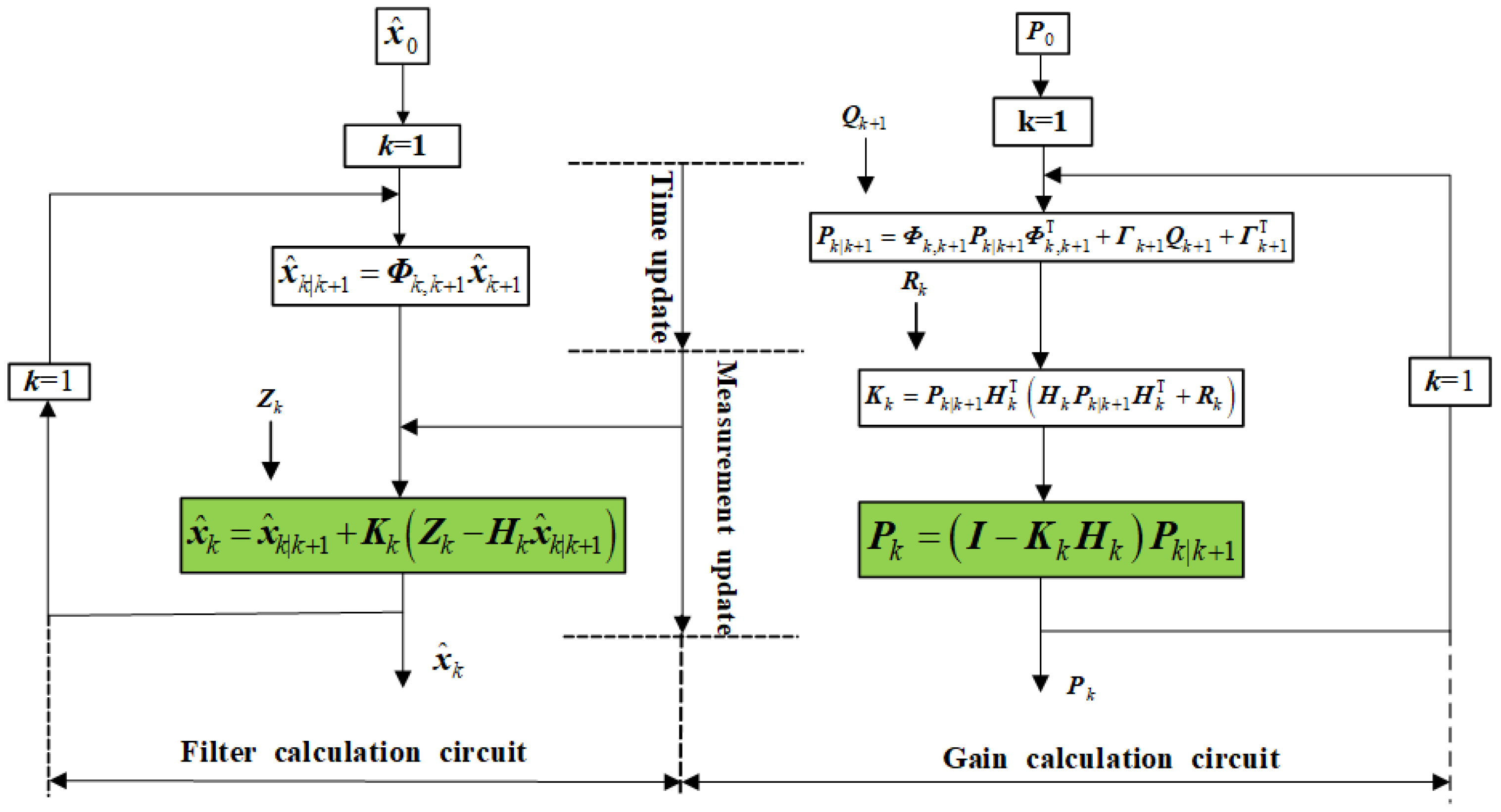
KF	(1) Linear System Assumption: The KF assumes both the system model and observation model are linear, with additive Gaussian noise. This linear–Gaussian assumption theoretically guarantees a globally optimal solution. (2) High Computational Efficiency: The KF exhibits low computational complexity (O(n2) for state dimension n), making it well-suited for real-time applications with stringent timing requirements. (3) Optimal Estimation Accuracy: Under strict adherence to linear–Gaussian assumptions, the KF provides statistically optimal estimates in the minimum mean-square error sense. (4) Limited Applicability: The KF’s strict linearity assumptions lead to significant estimation errors when applied to nonlinear systems, severely constraining its practical application scope.	It is suitable for scenarios where the system is linear and the noise follows a Gaussian distribution, such as in simple navigation and signal processing.
EKF	(1) Nonlinear system processing: The EKF approximates nonlinear problems by linearizing the nonlinear system model. (2) Moderate computational complexity: The computational complexity of the EKF is higher than the KF but lower than the UKF. (3) Limited accuracy: Due to the linearization process, the EKF may experience larger estimation errors in strongly nonlinear systems. (4) Jacobian matrix calculation: The EKF requires computation of the Jacobian matrices of the system model and observation model, which increases the algorithm’s complexity. (5) Broad applicability: The EKF is a widely used method for handling nonlinear systems and is suitable for moderate nonlinearity.	It is suitable for scenarios where the nonlinearity is not high and fast real-time processing is required. Due to its lower computational complexity, the EKF is well-suited for use in embedded systems with limited computational resources. When the initial state estimation is relatively accurate, the EKF can converge quickly and provide better estimation results.
UKF	(1) Strong nonlinear system processing capability: The UKF selects a set of deterministic sampling points (Sigma points) through the UT, enabling a more accurate approximation of the statistical properties of nonlinear systems. (2) No Jacobian matrices required: The UKF avoids the complex Jacobian matrix calculations required in the EKF, enhancing the algorithm’s stability and precision. (3) Higher computational complexity: The computational complexity of the UKF is higher than that of the EKF, but it generally remains within acceptable limits. (4) High accuracy: The UKF outperforms the EKF in strongly nonlinear systems, providing more accurate estimation results.	Suitable for scenarios involving nonlinear systems with Gaussian noise, such as complex target tracking and robotic navigation
PF	(1) Strong nonlinear and non-Gaussian adaptability: The PF is a recursive Bayesian estimation technique based on Monte Carlo methods, capable of handling complex nonlinear systems and non-Gaussian noise environments. It approximates the posterior probability distribution through a large number of random samples (particles), thus avoiding the linearity and Gaussian assumptions required by traditional filtering methods (e.g., KF). (2) Flexibility and robustness: The PF exhibits high flexibility, adapting to diverse systems and observation models. It demonstrates strong robustness against noise and outliers, making it particularly suitable for dynamic systems in complex environments. (3) Parallel computing capability: The computational process of the PF can be parallelized, as the prediction and update operations for each particle are executed independently, significantly improving computational efficiency. (4) Handling complex probability distributions: The PF can manage multimodal probability distributions, making it ideal for state estimation in complex scenarios. Through its particle weight updating mechanism, it effectively integrates information from multiple sensors. (5) Challenges and optimizations: Despite its adaptability, the PF faces challenges such as particle degeneracy and high computational complexity. To address these issues, researchers have proposed improvements like adaptive PF, combining the UKF to generate proposal distributions, and optimizing resampling strategies.	Suitable for nonlinear and non-Gaussian systems, such as target tracking, robotic navigation, and signal processing.
UPF	(1) Adaptability to non-Gaussian noise: When combined with a PF, the UKF further enhances its adaptability to non-Gaussian and multimodal probability distributions. (2) Balanced computational efficiency and accuracy: The UKF achieves a good balance between computational efficiency and accuracy. While its computational complexity is higher than that of the traditional KF, the UKF outperforms the EKF in handling high-dimensional state spaces and has lower computational complexity compared to the PF. By integrating a PF, particles are generated and updated via the UT, further improving particle effectiveness and sampling efficiency. (3) Mitigation of particle degeneracy: In PFs, particle degeneracy—a common issue where most particle weights approach zero, reducing the number of effective particles—is alleviated when combined with the UKF. Sigma points generated through the UT provide a more accurate description of the state distribution, thereby reducing particle degeneracy. (4) Further optimization via PF integration: The UPF combines the strengths of the UKF and the PF. By generating and updating particles through the UKF UT, UPF retains PF’s strong adaptability to nonlinear and non-Gaussian problems while improving sampling efficiency.	Suitable for nonlinear and non-Gaussian systems where high estimation accuracy is required.
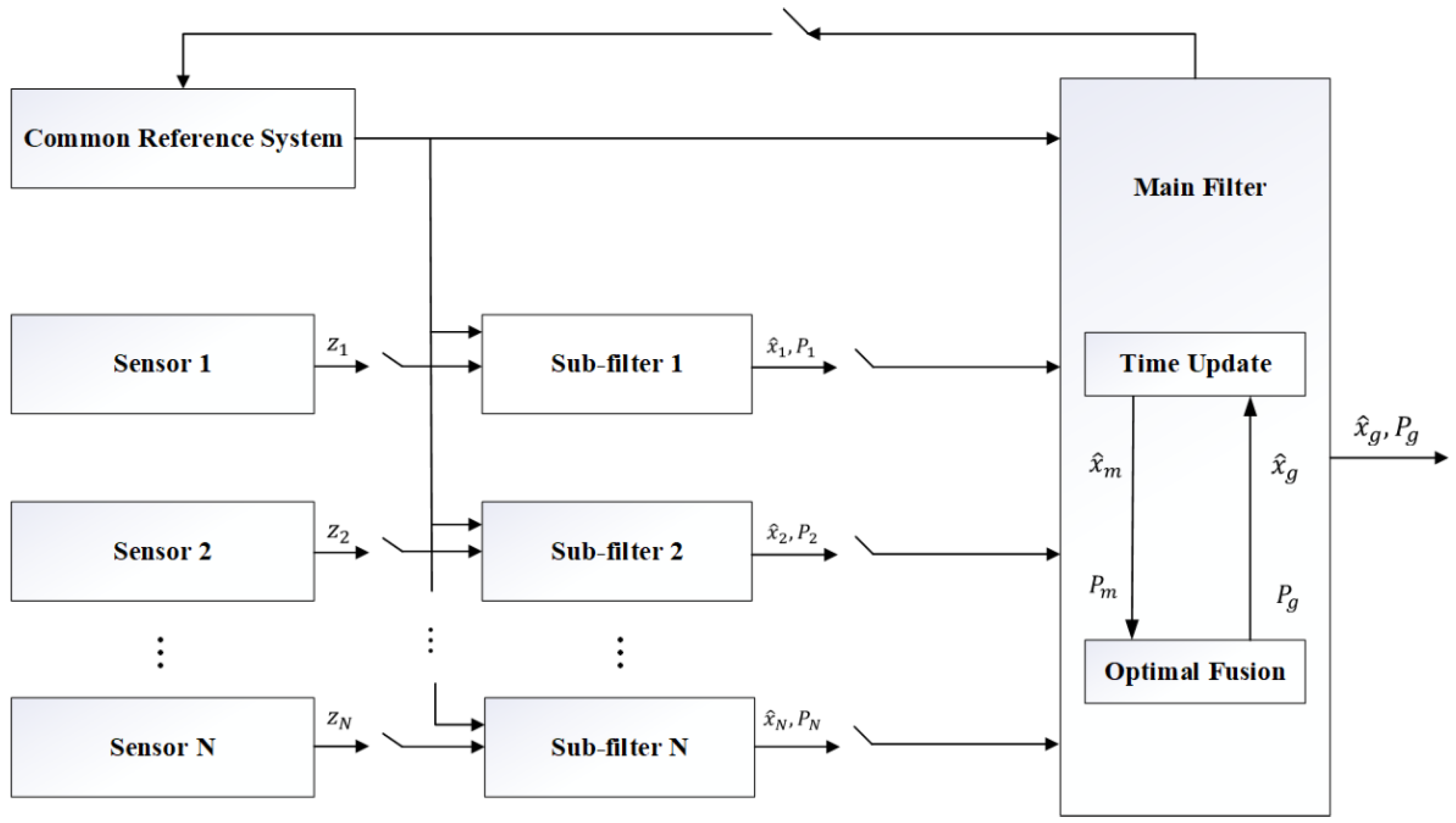
FF	(1) Distributed Structure and Flexibility: The FF adopts a distributed architecture, decomposing data fusion tasks into multiple sub-filters and a master filter. This structural design offers flexibility, allowing the selection of appropriate filtering algorithms (e.g., EKF, UKF) based on the characteristics of different sensors. It also supports dynamic adaptation to sensors joining or leaving the network. (2) Fault Tolerance and Fault Isolation Capability: The FF can detect and isolate faulty sensors in real time, preventing erroneous data from degrading global estimation accuracy. This ensures high precision and reliability even when partial sensor failures occur. (3) Diversity of Information Allocation Strategies: The FF supports multiple information allocation strategies, including zero-reset mode, variable proportion mode, feedback-free mode, and fusion-feedback mode. These strategies exhibit trade-offs in computational complexity, fusion accuracy, and fault tolerance, enabling flexible selection tailored to specific application scenarios. (4) High Computational Efficiency: By distributing data processing among multiple sub-filters, each of which handles only local data, the FF reduces the computational load. This distributed computing approach not only enhances the system’s real-time performance but also lowers the demand for hardware resources. (5) Adaptive and Dynamic Adjustment Capability: Integrated with adaptive filtering theory, the FF dynamically adjusts information allocation coefficients based on sensor performance and environmental changes. (6) Plug-and-Play Functionality: The FF supports plug-and-play operation for sensors, enabling rapid adaptation to dynamic sensor addition or removal. This feature enhances flexibility and adaptability in complex environments or evolving mission requirements. (7) Globally Optimal Estimation: The master filter synthesizes local estimates from sub-filters to achieve a globally optimal estimate. This two-tier architecture preserves local filtering precision while improving overall system performance through global fusion. (8) Suitability for Complex Environments: The FF excels in multi-source heterogeneous data fusion scenarios, such as integrating satellite navigation, inertial navigation, and visual navigation in navigation systems. It effectively addresses sensor noise, model biases, and environmental interference challenges.	Suitable for multi-sensor networks, especially in scenarios where sensors are widely distributed and communication resources are limited.
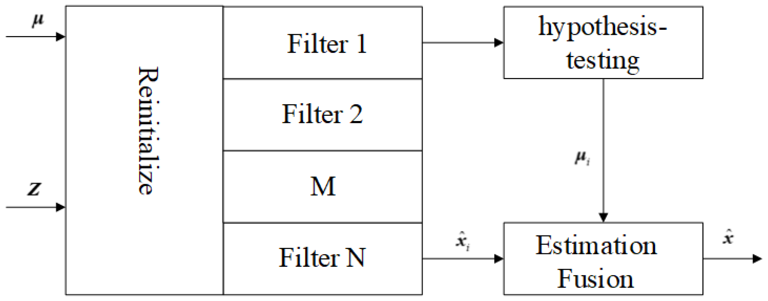
MME	(1) Multimodal Data Processing Capability: MME methods can handle data from different modalities, such as images, text, audio, and video. By mapping multimodal data into a unified feature space or integrating information through fusion techniques, these methods leverage the complementary nature of different modalities to enhance model performance. (2) Diversity of Fusion Strategies: MME methods support various fusion strategies, including early fusion (integration at the data level), mid-level fusion (integration at the feature level), late fusion (integration at the decision level), and hybrid fusion (combining multiple strategies). Different strategies are suited to different application scenarios, enabling flexible adaptation to complex data fusion requirements. (3) Enhanced Model Robustness: By incorporating multimodal data and multi-model estimation, uncertainties arising from single-modality data can be effectively reduced, improving the model’s robustness against noise and outliers. (4) Improved Performance and Generalization Capability: MME methods comprehensively capture target information by fusing multimodal data, thereby boosting both model performance and generalization ability. (5) Flexibility in Model Architecture: MME methods typically offer high flexibility, allowing the selection of appropriate model architectures based on specific task requirements. For example, unified embedding-decoder architectures and cross-modal attention architectures can be combined to fully exploit the advantages of different structural designs.	(1) In scenarios such as multi-object tracking and complex trajectory prediction, multi-model estimation methods can effectively deal with the various motion patterns and uncertainties of targets. (2) Suitable for integrated navigation systems, such as the fusion of inertial navigation and satellite navigation, multi-model estimation can improve positioning accuracy and reliability. (3) In complex industrial scenarios such as power systems and chemical processes, MME methods can be used for modeling and control to address the dynamic changes in system parameters.
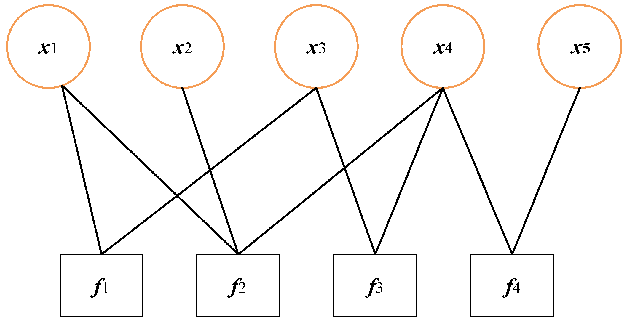
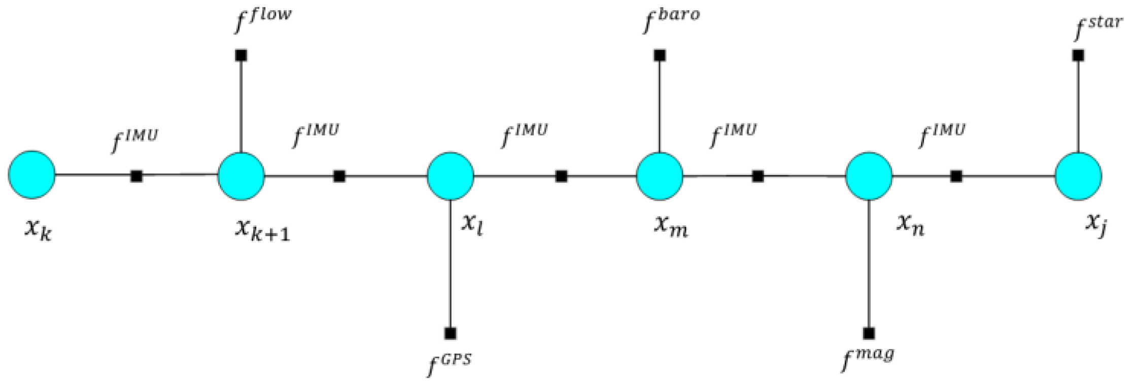
FG	(1) Intuitiveness and Flexibility: FGs visually represent the relationships between variables and factors, making complex probabilistic models more intuitive and easier to understand. Compared to Bayesian networks, FGs can more generally express the decomposition of probability distributions, making them suitable for a wide range of complex probabilistic models. (2) Efficient Inference and Optimization Capabilities: FGs excel in algorithms such as variable elimination and message passing, significantly improving inference efficiency. By jointly optimizing the relationships between data from different sensors, FGs can efficiently fuse multi-sensor data. (3) Strong Multi-Source Data Fusion Capability: FGs can effectively integrate data from various sensors (such as cameras, radars, and IMUs). By constructing an FG model, they can jointly optimize heterogeneous multi-source data, thereby enhancing the accuracy and reliability of data fusion. (4) Support for Dynamic Data Processing: FG algorithms support techniques such as sliding-window optimization (Sliding-Window FGO), enabling dynamic processing of real-time data streams. This makes them suitable for scenarios with high computational complexity and stringent real-time requirements. (5) Robustness and Outlier Resistance: In complex environments (such as urban canyons), FGO demonstrates better robustness and positioning accuracy compared to traditional methods like the EKF.	(1) Autonomous Driving and Robot Navigation: FG methods are widely used in autonomous driving and robot navigation to integrate data from multiple sources such as cameras, radar, LiDAR, and IMU, thereby enhancing the accuracy of localization and mapping. (2) Underwater Robot Localization: In complex underwater environments, FG methods can effectively handle abnormal sensor observations, thereby improving the positioning accuracy of Autonomous Underwater Vehicles. (3) Industrial Fault Detection and Diagnosis: FG methods can be used to integrate monitoring data from different sensors to achieve early warning and diagnosis of equipment faults. (4) Medical Diagnosis: In the medical field, FG methods can integrate patients’ medical records, imaging data, and laboratory test results to improve the accuracy of disease diagnosis. (5) Environmental Monitoring: FG methods can integrate data from satellites, ground sensors, and meteorological data to monitor environmental changes in real time, supporting environmental management and decision-making.
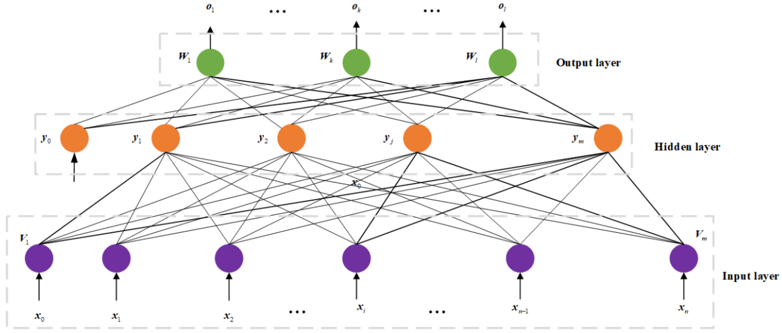
AI	(1) Heterogeneous Data Processing Capability: AI methods can handle data from diverse sources, formats, and structures (such as text, images, and sensor data) through multimodal models (e.g., Transformers, hybrid neural networks) to achieve unified processing. (2) Automatic Feature Extraction and Representation Learning: Deep learning models (e.g., autoencoders, BERT) autonomously learn high-level abstract features without manual feature engineering, adapting to the complexity of multi-source data. This reduces reliance on domain-specific knowledge while improving feature expression efficiency and generalization. (3) Robustness and Fault Tolerance: AI maintains stability amid data noise, missing values, or conflicts by leveraging adversarial training, data augmentation, and attention mechanisms to filter redundant information. (4) Additional capabilities include cross-modal association and reasoning, real-time performance and scalability, and adaptability and dynamic updating.	(1) Autonomous Driving: Integrating data from cameras, radar, and LiDAR helps vehicles understand their surroundings from multiple perspectives, enabling safe navigation. (2) Medical Diagnosis: Fusing patient medical records with medical imaging data allows for the rapid and accurate identification of diseases, thereby improving diagnostic efficiency. (3) Smart Cities: In real estate management, combining sensor data, social media feedback, and Geographic Information System (GIS) data optimizes urban spatial layout and resource allocation. (4) Industrial Internet of Things (IIoT): Analyzing sensor data enables predictive maintenance and optimization of equipment, thereby increasing production efficiency. (5) Environmental Monitoring: Integrating satellite data, ground sensor data, and meteorological data allows for real-time monitoring of environmental changes, supporting environmental management and decision-making.
Uncertainty reasoning	(1) Strong capability in handling uncertainty: Uncertainty reasoning methods can effectively deal with uncertainty in data, including imprecision, inconsistency, and sensor errors. For example, the Dempster–Shafer theory of evidence can model and fuse uncertain information, while Bayesian methods handle uncertainty through probabilistic updates. (2) High flexibility: Uncertainty reasoning methods can flexibly handle different types of data sources and meet the needs of fusing multi-source heterogeneous data. They are capable of integrating symbolic reasoning and numerical reasoning to process various types of information, ranging from qualitative to quantitative. (3) Enhanced decision-making reliability: By properly handling uncertainty, uncertainty reasoning methods can improve the reliability of the fusion results and provide support for decision-making in complex environments. (4) High computational complexity, high requirements for data preprocessing, difficulty in model construction, and challenges in real-time performance.	(1) Target Recognition and Tracking in Complex Environments: In target recognition and tracking tasks, uncertainty reasoning methods can effectively handle uncertain data from multiple sensors (such as cameras and radars), thereby improving the accuracy and reliability of target detection. (2) Medical Diagnosis: In the medical field, by integrating patients’ medical records, imaging data, and laboratory test results, uncertainty reasoning methods can more accurately identify diseases and enhance the accuracy of diagnosis.

5. Conclusions

This paper provides a detailed overview of various algorithms corresponding to multi-source fusion processing methods. It summarizes the fundamental principles of these algorithms and briefly introduces their mathematical models, key characteristics, and application scenarios, offering significant theoretical and technical support for intelligent navigation, driverless vehicles, autonomous navigation, and related fields. Due to limitations in theoretical understanding and technical conditions, all existing fusion algorithms exhibit shortcomings. Currently, no single fusion algorithm can fully meet the requirements of multi-source integrated navigation systems. Therefore, appropriate fusion algorithms must be selected based on practical needs and application contexts. The historical development of these fusion algorithms reveals their interdisciplinary nature, combining theories and methodologies from integrated navigation, GNSS data processing, satellite geodesy, probability theory and mathematical statistics, computer science, statistics, and artificial intelligence. Consequently, multi-source integrated navigation algorithms should not be confined to traditional positioning and navigation approaches. Instead, they should continuously incorporate insights from other disciplines, foster mutual learning and advancement across fields, and generate innovative theories and methods through interdisciplinary integration. This evolution aims to deliver high-precision, high-reliability positioning, navigation, and timing services across all temporal and spatial domains—representing the future development trend of multi-source integrated navigation systems.