A Novel Hybrid Approach Using an Attention-Based Transformer + GRU Model for Predicting Cryptocurrency Prices

Abstract

In this article, we introduce a novel deep learning hybrid model that integrates attention Transformer and gated recurrent unit (GRU) architectures to improve the accuracy of cryptocurrency price predictions. By combining the Transformer’s strength in capturing long-range patterns with GRU’s ability to model short-term and sequential trends, the hybrid model provides a well-rounded approach to time series forecasting. We apply the model to predict the daily closing prices of Bitcoin and Ethereum based on historical data that include past prices, trading volumes, and the Fear and Greed Index. We evaluate the performance of our proposed model by comparing it with four other machine learning models, two are non-sequential feedforward models: radial basis function network (RBFN) and general regression neural network (GRNN), and two are bidirectional sequential memory-based models: bidirectional long short-term memory (BiLSTM) and bidirectional gated recurrent unit (BiGRU). The model’s performance is assessed using several metrics, including mean squared error (MSE), root mean squared error (RMSE), mean absolute error (MAE), and mean absolute percentage error (MAPE), along with statistical validation through the non-parametric Friedman test followed by a post hoc Wilcoxon signed-rank test. Results demonstrate that our hybrid model consistently achieves superior accuracy, highlighting its effectiveness for financial prediction tasks. These findings provide valuable insights for enhancing real-time decision making in cryptocurrency markets and support the growing use of hybrid deep learning models in financial analytics.

1. Introduction

The cryptocurrency market has grown exponentially, with Bitcoin and Ethereum standing out as the top 2 dominant digital assets. Both of these account for the majority of trading activity and significantly impact global financial trends. One of the biggest challenges in working with cryptocurrencies is figuring out how to develop accurate models that can predict their highly volatile prices. Numerous studies have shown that machine learning (ML) models are highly effective in predicting cryptocurrency prices, as they can capture complex nonlinear patterns in financial time series [1,2,3,4,5,6,7,8,9]. Among these, artificial neural network (ANN)-based machine learning algorithms, such as radial basis function network (RBFN), general regression neural network (GRNN), gated recurrent unit (GRU), and long short-term memory (LSTM), have been widely applied in this field.

Broomhead and Lowe [10,11] introduced the radial basis function networks (RBFNs) to model complex relationships between features and target variables and to make predictions on new data. RBFNs are a type of simple feedforward neural network that utilizes radial basis functions as their activation functions. One of the key benefits of using radial basis functions in RBFNs is their ability to smooth out non-stationary time series data while effectively still modeling the underlying trends. Alahmari [12] compared using the linear, polynomial, and radial basis function (RFB) kernels in the support vector regression for predicting the prices of Bitcoin, XRP, and Ethereum and showed that the RFB outperforms the other kernel methods in terms of accuracy and effectiveness. Recently, Casillo et al. [13] showed that the RRBFn models are effective in predicting Bitcoin prices from the analysis of online discussion sentiments. More recently, Zhang [14] demonstrated that combining a radial basis function (RBF) with a battle royale optimizer (BRO) significantly enhances the accuracy of stock price predictions, including those for cryptocurrencies. The results of his study showed that this approach outperformed other machine learning models like LSTM, BiLSTM-XGBoost, and CatBoost.

The general regression neural network (GRNN) is another type of feedforward neural network that was first proposed by Specht [15] designed for efficient use in regression tasks. One of the key strengths of GRNN is its ability to model complex nonlinear relationships without the need for iterative training. This has made it a powerful tool for applications in regression, prediction, and classification. Despite its advantages, GRNN’s application in cryptocurrency prediction is still relatively not widely explored [16,17]. In this article, we try to fill in the gap by assessing the performance of GRNN in predicting the prices of Bitcoin and Ethereum.

Recurrent neural networks (RNNs) are designed for handling sequential data because, unlike feedforward neural networks, they have feedback loops that enable them to retain information from previous inputs using a method called backpropagation through time (BPTT). However, when training on long sequences, the residual error gradients that need to be propagated back diminish exponentially due to repeated multiplication of small weight across time steps. This makes it difficult for the network to learn long-term dependencies. To address such a problem and to improve the modeling of long-term dependencies in sequential data, Hochreiter and Schmidhuber [18] proposed the long short-term memory (LSTM) network model. The LSTM model has been widely adopted in the literature, as it has proven to be highly effective in forecasting cryptocurrency prices, outperforming other machine learning models [19,20,21]. Lahmiri and Bekiros [22] showed that the Bitcoin, Digital Cash, and Ripple price predictability of LSTM is significantly higher when compared with that of GRNN. Ji et al. [23] conducted a comparative study comparing the LSTM network model with deep learning network, convolutional neural network, and deep residual network models for predicting the Bitcoin prices and showed that the LSTM slightly outperformed the other models for regression problems, whereas for classification (up and down) problems, the deep learning network works the best. Uras et al. [24] used LSTM to predict the daily closing price series of Bitcoin, Litecoin and Ethereum cryptocurrencies based on the prices and volumes of prior days and showed that the LSTM outperformed the traditional linear regression models. Lahmiri and Bekiros [25] conducted a study comparing the performances of LSTM and GRNN models in predicting Bitcoin, Digital Cash, and Ripple prices. Their findings indicated that the LSTM model outperformed GRNN in terms of prediction accuracy.

The gated recurrent unit (GRU) neural network model, introduced by Cho et al. [26], was designed to handle long-term dependencies in sequential data, similar to the LSTM model, but with fewer parameters, making GRU computationally less expensive and faster than LSTM [27]. Dutta et al. [28] used GRU to predict the prices of cryptocurrencies and demonstrated that the GRU outperformed the LSTM networks. Tanwar et al. [29] employed GRU and LSTM to predict the price of Litecoin and Zcash cryptocurrencies, taking into account the inter-dependency of the parent coin. Their findings showed that these models forecasted the prices with high accuracy compared with other machine learning models. Ye et al. [30] proposed a method combining LSTM and GRU to predict the prices of Bitcoin using the historical transaction data, sentiment trends of Twitter, and technical indicators, and showed that their method can better assist investors in making the right investment decision. Patra and Mohanty [31] developed a multi-layer GRU network model with multiple features to predict the prices of Bitcoin, Ethereum, and Dogecoin, and demonstrated that their model provided better performance compared with the LSTM and GRU models that used a single feature.

Several studies have shown that bidirectional long short-term memory (BiLSTM) and bidirectional gated recurrent unit (BiGRU) enhance the accuracy of financial time series predictions. Unlike traditional LSTM and GRU, these bidirectional models process data in both forward and backward directions, allowing for capturing dependencies from past and future time steps. For example, Hansun et al. [32] compared three popular deep learning architectures, LSTM, bidirectional LSTM, and GRU, for predicting the prices of five cryptocurrencies, Bitcoin, Ethereum, Cardano, Tether, and Binance Coin, using various prediction models. Their findings indicated that BiLSTM and GRU performed just as well as LSTM, offering robust and accurate predictions of cryptocurrency prices. Ferdiansyah et al. [33] showed that combining GRU and BiLSTM in a hybrid model increased prediction accuracy for Bitcoin, Ethereum, Ripple, and Binance.

In this article, we propose a novel Hybrid Transformer + GRU model and compare its performance with two non-sequential feedforward models (GRNN and RBFN) and two bidirectional sequential memory-based models (BiGRU and BiLSTM) for forecasting cryptocurrency prices across two distinct modeling scenarios. The first scenario aims to predict Bitcoin prices using historical Bitcoin price data, its trading volume, and crypto Fear and Greed Index (FGI). The second scenario aims to predict Ethereum prices using historical price data for both Bitcoin and Ethereum, along with Ethereum’s trading volume and the Fear and Greed Index (FGI). The Transformer model, introduced by Vaswani et al. [34], revolutionized natural language processing (NLP) by using self-attention and feedforward networks. Since then, Transformers have been adapted and extended in numerous ways and became the foundation for AI systems like ChatGPT and DeepSeek [35,36]. The application of Transformer neural networks to financial time series data is a promising area of research [37,38,39,40]. For example, Li et al. [41] successfully applied Transformers to forecast both synthetic and real-world time series data. Their work demonstrated that Transformers excel at capturing long-term dependencies, an area where LSTMs often struggle. Zerveas et al. [42] demonstrated that the transformer-based approach for unsupervised pre-training on multivariate time series outperforms traditional methods for both regression and classification tasks, even with smaller datasets. Wu et al. [43] developed an Autoformer model based on decomposing Transformers with an autocorrelation mechanism to better handle long-term forecasting and seasonality in complex time series. They showed that their model outperformed traditional approaches, delivering more accurate results. A recent work by Castangia et al. [44] highlights how effective Transformer models are for flood forecasting, outperforming traditional recurrent neural networks (RNNs). More recently, Nayak et al. [45] proposed a user-friendly Python 3.11.9 code that implements Transformer architecture specifically for time series forecasting data.

To the best of our knowledge, this is the first study to introduce a deep learning model that combines a parallel self-attention-based Transformer architecture with a sequential memory-based GRU model. This unique combination enables our model to effectively capture both long-term dependencies through the Transformer’s self-attention mechanism and short-term temporal patterns using the GRU’s gated memory. This makes the model well suited to capturing market dynamics across different timescales, especially during volatile periods. The rest of this article is organized as follows: Section 2 defines the prediction models used to predict Bitcoin and Ethereum prices. Here, we define four neural network models that we need to compare with our proposed model. Two of these four models are classified as feedforward neural networks, and the other two are classified as memory-based models. Section 3 introduces our new deep learning approach for cryptocurrency price prediction. Section 4 presents the data and results, showcasing how all five models perform in this comparative study. Finally, Section 5 summarizes our findings and draws some conclusions and recommendations.

2. Prediction Models

We consider modeling the cryptocurrency prices as a function of past feature values with a one-time-step lag, as follows:

$$y_t=f\left({\mathbf{x}}_{t-1}\right)+{\epsilon }_t,$$

(1)

where $y_t$ is the target variable representing the price of Bitcoin or Ethereum at time t, $f\left({\mathbf{x}}_{t-1}\right)$ is a function of the features ${\mathbf{x}}_{t-1}$ at time $t-1$ that need to be approximated, and ${\epsilon }_t$ is the error term representing the difference between the predicted price and the actual price at time t. Here, we consider ${\mathbf{x}}_{t-1}$ as a three-dimensional vector representing the prices (USD) of Bitcoin/Ethereum, $P_{t-1}$; exchange trading volume (USD), $V_{t-1}$, of Bitcoin/Ethereum; and Fear and Greed Index (FGI), $F_{t-1}$, at time $t-1$.

We use the following four different networks along with our proposed model to forecast the prices of Bitcoin and Ethereum given in Equation (1).

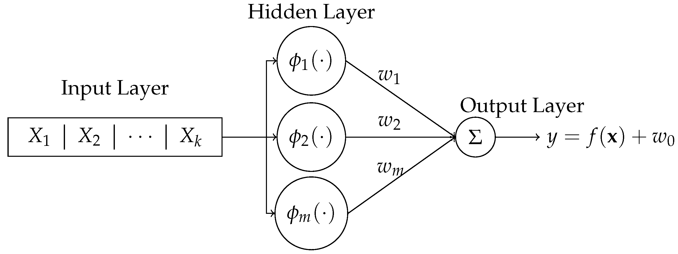
2.1. Radial Basis Function Network (RBFN)

A radial basis function network (RBFN) is a type of feedforward neural network that uses radial basis functions as activation functions. Typically, it consists of three layers, as shown in Figure 1: the input layer, which receives the input data; the hidden layer, which applies radial basis functions, such as Gaussian activation (kernel) functions, to transform the input data into a higher-dimensional space; and the output layer, which produces the final output, often as a linear combination of the hidden layer outputs.

Mathematically, the input can be considered as a vector of k variables $\mathbf{x}={(X_1,X_2,\cdots ,X_k)}^{\top }$, each with n observations. The kernel function is used as the activation function in the hidden layer. Typically, the most common choice is the Gaussian function, as follows:

$$\phi \left(\mathbf{x},{\mathbf{c}}_i\right)=exp\left(-{\displaystyle \frac{{∥\mathbf{x}-{\mathbf{c}}_i∥}^2}{2{\sigma }_i^2}}\right)$$

(2)

where $\left|\right|\mathbf{x}-{\mathbf{c}}_i\left|\right|$ is the Euclidean distance between the input vector $\mathbf{x}$ and the center ${\mathbf{c}}_i=(c_{i1},c_{i2},\cdots ,c_{ik})$, and ${\sigma }_i$ is the bandwidth or spread parameter. The output of the hidden layer is passed to the output layer, where the final output is computed as a linear combination of the hidden layer outputs, as follows:

$$y=\sum _{i=1}^m{w}_i\phi \left(\mathbf{x},{\mathbf{c}}_i\right)+w_0$$

(3)

where m denotes the number of neurons in the hidden layer, ${\mathbf{c}}_i$ is the center vector for neuron i, $w_i$ is the weight of neuron i in the linear output neuron, $w_0$ is the bias term, and $\phi$ is the activation function (radial basis function) for the $i^{\mathrm{th}}$ RBF neuron.

2.2. General Regression Neural Network (GRNN) Model

The general regression neural network (GRNN), introduced by Specht [15], is another type of feedforward neural network that is designed for regression tasks and closely related to the radial basis function (RBF) network. Unlike traditional feedforward and deep neural networks, GRNN does not rely on backpropagation or gradient-based optimization. Instead, it operates by minimizing the difference between predicted and actual target values. The model directly memorizes the training data and leverages them for predictions.

GRNN comprises three layers: the input layer, hidden layer, and output layer. The set of n training data ${\{{\mathbf{x}}_i,y_i\}}_{i=1}^n$ enters the input layer as a set of k features $\mathbf{x}$ and their associated target y. Then the hidden layer uses a kernel function to compute the similarity between a new input feature $\mathbf{x}$ and each training sample ${\mathbf{x}}_i$. The Gaussian kernel is commonly used, as follows:

$$K\left(\mathbf{x},{\mathbf{x}}_i\right)=exp\left(-{\displaystyle \frac{{∥\mathbf{x}-{\mathbf{x}}_i∥}^2}{2{\sigma }_i^2}}\right),$$

(4)

where $\mathbf{x},{\mathbf{x}}_i$, and ${\sigma }_i$ are the new input vector, the training sample, and the smoothing parameter, respectively. Then it gives a set of weights associated with the closeness distance, as follows:

$$w_i={\displaystyle \frac{exp\left(-\frac{{∥\mathbf{x}-{\mathbf{x}}_i∥}^2}{2{\sigma }_i^2}\right)}{{\sum }_{i=1}^{n}exp\left(-\frac{{∥\mathbf{x}-{\mathbf{x}}_i∥}^2}{2{\sigma }_i^2}\right)}}.$$

(5)

Finally, the output layer computes the prediction value of y as a weighted average of nearby observations, as follows:

$$\widehat{y}=\sum _{i=1}^n{w}_i{y}_i$$

(6)

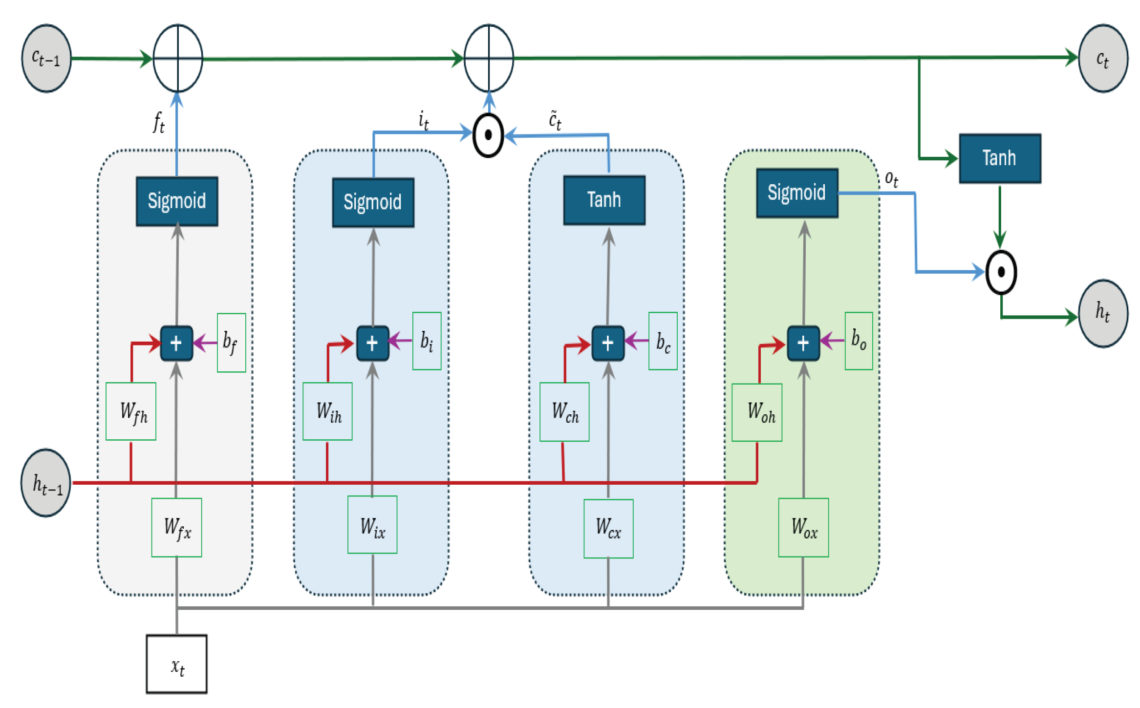
2.3. Long Short-Term Memory (LSTM) Model

Long short-term memory (LSTM) is a specialized type of recurrent neural network (RNN) developed to solve the vanishing gradient problem that standard RNNs often faced. This problem makes it challenging for the model to capture long-term dependencies when dealing with long sequences. To overcome this limitation, LSTM uses a memory cell designed to store information over extended periods while discarding irrelevant details. Figure 2 illustrates the structure of the LSTM.

The first step of the LSTM network is to decide what information will be discarded from the memory cell state $c_{t-1}$. The sigmoid activation function in the forget gate is applied to the current input, $X_t$, and the output from the previous hidden state, $h_{t-1}$, and produces values between 0 and 1 for each element in the cell state. A value of 1 indicates “keep this information”, while a value of 0 means “omit this information”, as follows:

$$\mathrm{Forget}\mathrm{gate}:f_t=\sigma \left(W_{fx}{X}_t+W_{fh}{h}_{t-1}+b_f\right)$$

(7)

where $W_{fx}$ and $W_{fh}$ represent the weight matrices for the input and recurrent connections, respectively, and $b_f$ denotes the bias vector parameters.

The next step decides what new information will be stored in the cell state. The input gate first applies the sigmoid layer to the input from the previous hidden state and the input from the current state to determine which parts of the information should be updated. Then, a tanh layer generates a new candidate value, ${\tilde{c}}_t$, that could potentially be added to the cell state, as follows:

$$\begin{array}{cc}\hfill \mathrm{Input}\mathrm{gate}:i_t& =\sigma \left(W_{ix}{x}_t+W_{ih}{h}_{t-1}+b_i\right)\hfill \end{array}$$

(8)

$$\begin{array}{cc}\hfill \mathrm{Intermediate}\mathrm{cell}\mathrm{state}:\widetilde{c_t}& =tanh\left(W_{cx}{x}_t+W_{ch}{h}_{t-1}+b_c\right)\hfill \end{array}$$

(9)

where W and b are weight matrices and bias vector parameters. Following this, the previous cell state $c_{t-1}$ is updated by a new cell state $c_t$, as follows:

$$\mathrm{New}\mathrm{cell}\mathrm{state}:c_t=f_t\odot c_{t-1}+i_t\odot {\tilde{c}}_t$$

(10)

where ⊙ denotes the Hadamard product (element-wise product).

Lastly, the model determines the final output, which is derived from the updated cell state after applying a filtering process: First, a sigmoid layer decides which portions of the cell state will be included in the output. Next, the cell state is passed through a tanh activation function to scale its values between $-1$ and 1, and the result is multiplied by the output gate to produce the final output.

$$\begin{array}{cc}\hfill \mathrm{Output}\mathrm{gate}:o_t& =\sigma \left(W_{ox}{x}_t+W_{oh}{h}_{t-1}+b_o\right)\hfill \end{array}$$

(11)

$$\begin{array}{cc}\hfill \mathrm{New}\mathrm{state}:h_t& =o_t\odot tanh\left(c_t\right)\hfill \end{array}$$

(12)

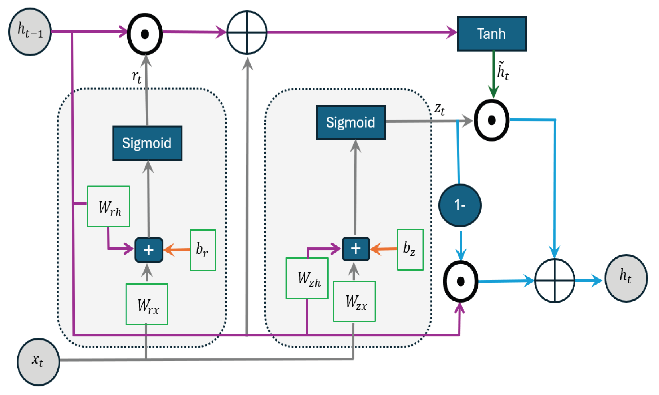
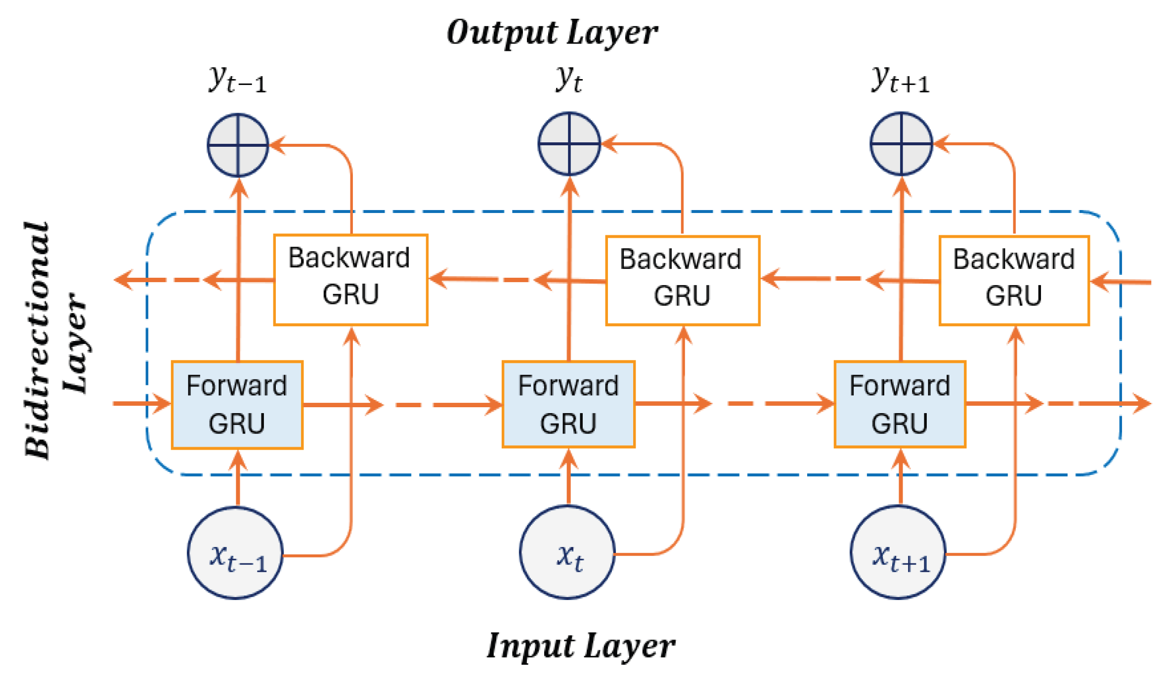
2.4. Gated Recurrent Unit (GRU) Model

The gated recurrent unit (GRU) has a simpler design than the LSTM network while still being effective at capturing long-term dependencies and handling the vanishing gradient problem we face in using RNN Cho et al. [26]. It uses two gates: the reset gate and update gate. The reset gate determines how much of the previous hidden state $h_{t-1}$ should be discarded when computing the new candidate hidden state ${\tilde{h}}_{t-1}$. The update gate controls how much of the new candidate hidden state, ${\tilde{h}}_{t-1}$, should be used to update the current hidden state.

Figure 3 illustrates the structure of the GRU, while Equations (13)–(16) explain its functionality mathematically as follows:

$$\begin{array}{cc}\hfill \mathrm{Reset}\mathrm{gate}:& r_t=\sigma \left(W_{rx}{x}_t+W_{rh}{h}_{t-1}+b_r\right)\hfill \end{array}$$

(13)

$$\begin{array}{cc}\hfill \mathrm{Update}\mathrm{gate}:& z_t=\sigma \left(W_{zx}{x}_t+W_{zh}{h}_{t-1}+b_z\right)\hfill \end{array}$$

(14)

$$\begin{array}{cc}\hfill \mathrm{Cell}\mathrm{state}:& {\tilde{h}}_t=tanh\left(W_x{x}_t+W_h\left(r_t\odot h_{t-1}\right)+b\right)\hfill \end{array}$$

(15)

$$\begin{array}{cc}\hfill \mathrm{New}\mathrm{state}:& h_t=z_t\odot {\tilde{h}}_t+\left(1-z_t\right)\odot h_{t-1}\hfill \end{array}$$

(16)

where $x_t$ denotes the input at the current state, $h_{t-1}$ represents the hidden state at the previous state, $r_t$ signifies the output of the reset gate, and $z_t$ corresponds to the output of the update gate. The symbol ⊙ stands for the Hadamard product, which is an element-wise multiplication operation, and ${\tilde{h}}_t$ denotes the candidate hidden state. Additionally, $W_x$ and $W_h$ refer to the feedforward and recurrent weight matrices, respectively, while b represents the bias parameters.

As shown in Figure 3 and Equations (13)–(16), the reset gate applies the sigmoid activation function to a linear combination of the current state, the output from the previous state, and a bias term. This helps determine how much information should be discarded. Similarly, the update gate uses the sigmoid function on a different linear combination of the current state, the previous output, and a bias term to decide how much information should be updated. The tanh activation function is then used to generate a new candidate value, ${\tilde{h}}_t$. This candidate is multiplied (using the Hadamard product) by the output from the update gate. Meanwhile, the difference value of the update state from 1 is multiplied by the previous output (again using the Hadamard product), and this result is added to the first product to produce the final output.

Research has demonstrated that processing the input sequences in both forward and backward directions can improve the accuracy of time series predictions. In our analysis, we will consider the two bidirectional models: the bidirectional long short-term memory (BiLSTM) and the bidirectional gated recurrent unit (BiGRU). Figure 4 shows the architecture of BiGRU. BiLSTM follows the same architecture as BiGRU, as shown in Figure 4, replacing the word “GRU” with “LSTM”. The forward pass in BiLSTM and BiGRU processes the sequence from $t=1$ to $t=n$, while the backward pass processes the sequence from $t=n$ to $t=1$. This bidirectional architecture allows these models to capture dependencies from past and future time steps, leading to improved prediction performance.

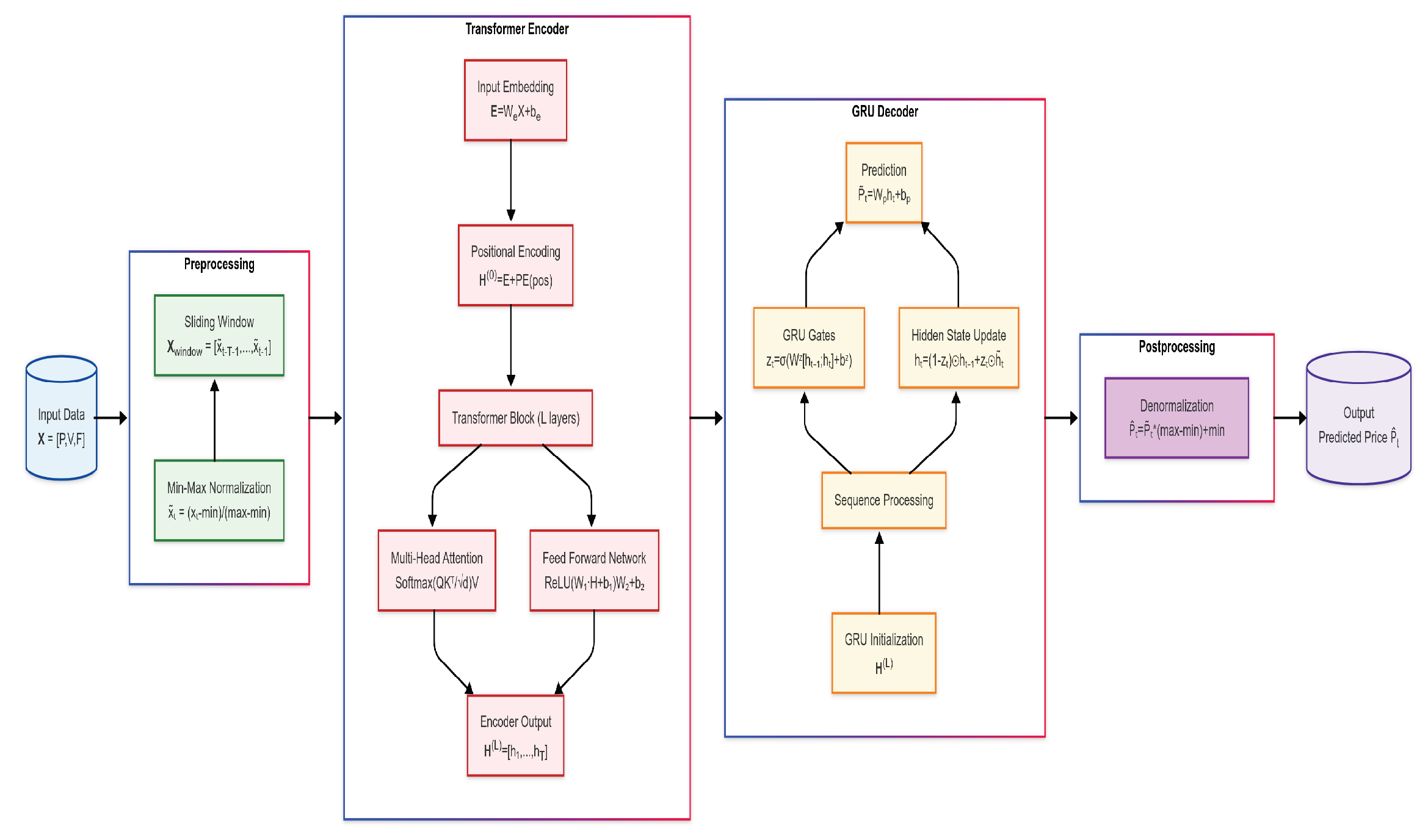
3. Hybrid Transformer + GRU Architecture

Transformer neural networks, introduced by Vaswani et al. [34] in their seminal 2017 paper “Attention Is All You Need”, have revolutionized the field of natural language processing (NLP). Unlike traditional sequential models like LSTM and GRU, transformers use self-attention to model relationships between all elements in a parallel sequence simultaneously, rather than processing them step by step. This architecture allows transformers to handle both local and global dependencies without the need for recurrent connections more efficiently. The transformers follow an encoder–decoder architecture, where both consist of multiple identical layers. The encoder processes the input, and the decoder produces the output. By leveraging the strengths of Transformer and gated recurrent unit deep learning models, we propose a new Hybrid Transformer + GRU model for cryptocurrency price prediction.

Step-by-Step Methodology

Below is a step-by-step algorithm of how the Hybrid Transformer + GRU model works:

1. 

Input features: At each time i,

$$x_i=\left[P_i,V_i,F_i\right]\in {\mathbb{R}}^3,$$

where $P_i,V_i,F_i$ are the price of Bitcoin/Ethereum, exchange trading volume of Bitcoin/Ethereum, and Fear and Greed Index, respectively.

2. 

Preprocessing:

2.1.

Normalization (Min–Max): Scale input features to the range $\left[0,1\right]$ using min–max normalization to ensure equal feature weighting.

$${\tilde{x}}_i={\displaystyle \frac{x_i-min\left(x\right)}{max\left(x\right)-min\left(x\right)}}$$

2.2.

Windowing: Split data into training and testing data and obtain a sliding window of values with fixed-length T (shape: $T\times 3$).

$$X_{\mathrm{window}}=\{{\tilde{x}}_{t-T-1},{\tilde{x}}_{t-T},\cdots ,{\tilde{x}}_{t-1}\}$$

3. 

Encoder (Transformer):

3.1.

Embedding layer: Project each ${\tilde{x}}_i$ into high-dimensional vectors d

$$E_i=W_e{\tilde{x}}_i+b_e,i=\{t-T-1,\cdots ,t-1\}$$

where $W_e\in {\mathbb{R}}^{d\times 3}$, $b_e\in {\mathbb{R}}^d$.

3.2.

Positional encoding: Add time-order information to embeddings (positional encodings) using sine/cosine waves of varying frequencies.

$$\begin{array}{c}P{E}_{(\mathrm{pos},2k)}=sin\left({\displaystyle \frac{\mathrm{pos}}{{10000}^{2k/d}}}\right),P{E}_{(\mathrm{pos},2k+1)}=cos\left({\displaystyle \frac{\mathrm{pos}}{{10000}^{2k/d}}}\right)\\ H_i^{\left(0\right)}=E_i+P{E}_i\end{array}$$

3.3.

Transformer layers: For each layer $\ell \in \{1,\cdots ,L\}$:

3.3.1.

Multi-head self-attention: For each head m, split $H^{(\ell -1)}$ into h heads

$${\mathrm{Attention}}_m=Softmax\left({\displaystyle \frac{Q_m{K}_m^T}{\sqrt{d_k}}}\right)V_m,$$

where

$$Q_h=H^{(\ell -1)}{W}_m^Q,K_m=H^{(\ell -1)}{W}_m^K,V_m=H^{(\ell -1)}{W}_m^V,d_k=d/h.$$

3.3.2.

 Concatenate heads:

$$MultiHead=\mathrm{Concat}\left[{\mathrm{Attention}}_1,\cdots ,{\mathrm{Attention}}_h\right]W^O$$

where $W^O\in {\mathbb{R}}^{h·d_v\times d}$.

3.3.3.

 Residual connections and LayerNorm: In deeper layers, each module is wrapped with a residual connection followed by layer normalization, as follows:

$$H_{\mathrm{attn}}^{(\ell )}=LayerNorm(H^{(\ell -1)}+MultiHead)$$

3.3.4.

 Feedforward Network (FFN): Non-linear transformation of features:

$$H_{\mathrm{ffn}}^{(\ell )}=ReLU\left(H_{\mathrm{attn}}^{(\ell )}{W}_1+b_1\right)W_2+b_2$$

where $W_1\in {\mathbb{R}}^{d\times d_{\mathrm{ffn}}}$ and $W_2\in {\mathbb{R}}^{d_{\mathrm{ffn}\times d}}$.

3.3.5.

 Second residual connections and LayerNorm:

$$H^{(\ell )}=LayerNorm\left(H_{\mathrm{attn}}^{(\ell )}+H_{\mathrm{ffn}}^{(\ell )}\right)$$

4. 

Decoder (GRU with attention):

4.1.

Sequence modeling: Process the Transformer’s final-layer output with GRU cells.

$$H^{\left(L\right)}=\{H_{t-T-1}^{\left(L\right)},\cdots ,H_{t-1}^{\left(L\right)}\}.$$

The GRU equations:

$$\begin{array}{c}{z}_i=\sigma \left(W_z[h_{i-1},H_i^{\left(L\right)}]\right)\left(\mathrm{Update}\mathrm{gate}\right)\\ r_i=\sigma \left(W_r[h_{i-1},H_i^{\left(L\right)}]\right)\left(\mathrm{Reset}\mathrm{gate}\right)\\ {\tilde{h}}_i=tanh\left(W_h[r_i\odot h_{i-1},H_i^{\left(L\right)}]\right)\left(\mathrm{Candidate}\mathrm{state}\right)\\ h_i=\left(1-z_i\right)\odot h_{i-1}+z_i\odot {\tilde{h}}_i\left(\mathrm{Hidden}\mathrm{state}\right)\end{array}$$

4.2.

Prediction: Use the final GRU hidden state $h_{t-1}$ to predict the price ${\widehat{P}}_t$:

$${\tilde{P}}_t=W_p{h}_{t-1}+b_p,$$

where $W_p\in {\mathbb{R}}^{1\times d_{\mathrm{gru}}}$ and $b_p\in \mathbb{R}$.

5. 

Output (post-processing): Convert predictions back (denormalization) to original price scale.

$${\widehat{P}}_t^{\mathrm{original}}={\tilde{P}}_t.\left(P_{max}-P_{min}\right)+P_{min}$$

Figure 5 illustrates the structure of this model. The main idea of our proposed model is to treat the historical cryptocurrency prices, trading volumes, and the Fear and Greed Index as a sequence of tokens, leveraging the self-attention mechanism to capture long-range dependencies while using GRU to detect sequential patterns and short-term fluctuations across different time steps. As shown in Figure 5, the historical data are first encoded as input tokens; then they go through embedding and positional encoding before entering the Transformer layers. The encoder outputs are fed into the GRU decoder, which applies attention over the encoder’s memory to make predictions.

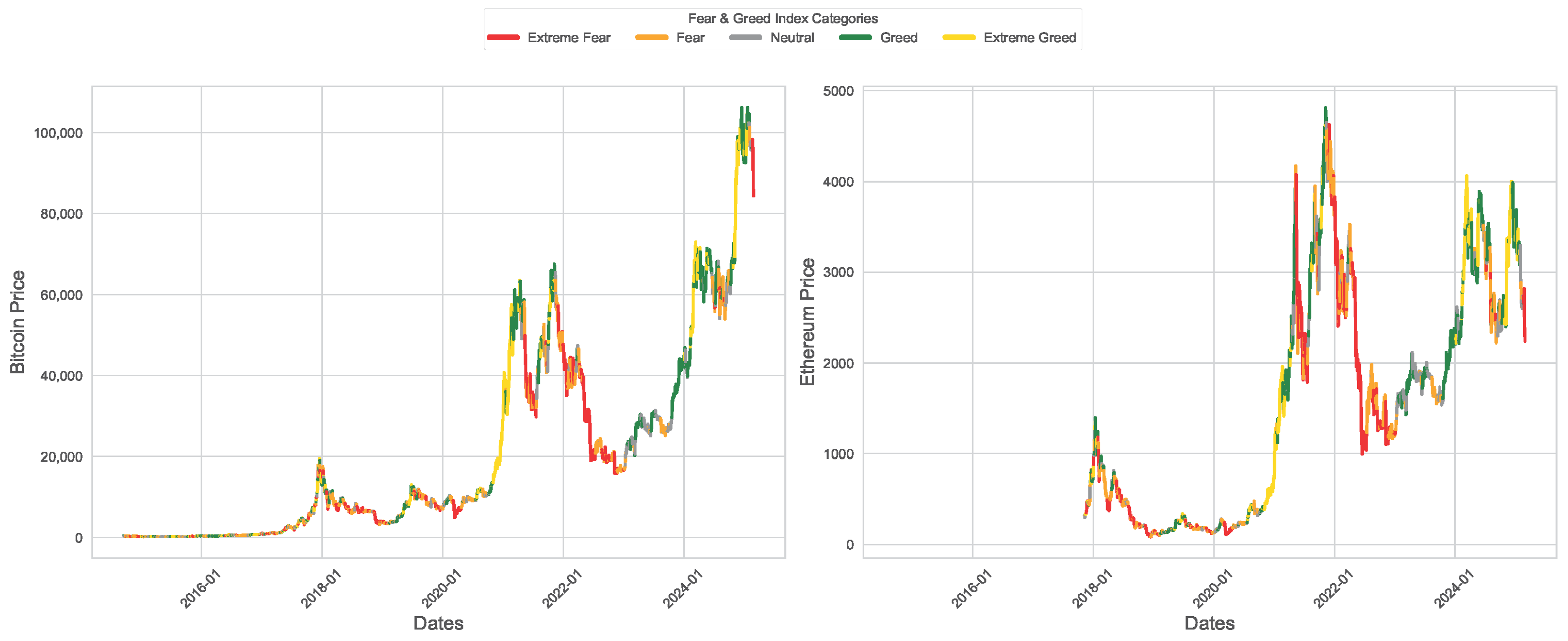
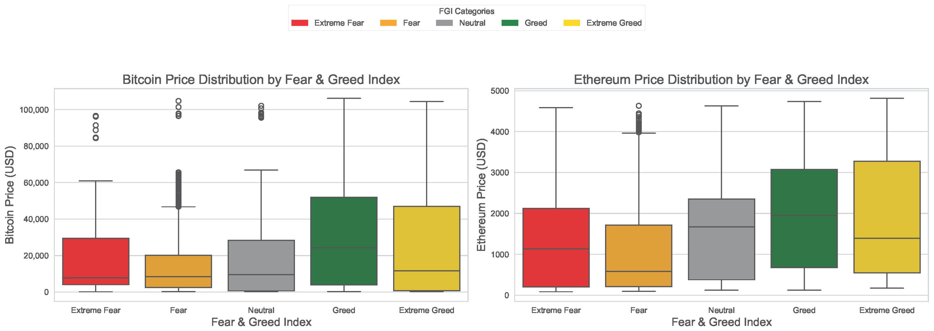
4. Exploratory Data Analysis

In our analysis, we consider the top 2 prominent cryptocurrencies with the highest cryptocurrency market capitalization: Bitcoin and Ethereum. The daily data were downloaded from the website https://coinmarketcap.com (last accessed on 4 April 2025), where we consider the daily closing prices and the trading exchange volume in USD for both digital assets.

Table 1. Historical data of Bitcoin and Ethereum prices.

Cryptocurrency	Start Date	End Date	Number of Records
Bitcoin	September 17, 2014	February 28, 2025	3818
Ethereum	November 09, 2017	February 28, 2025	2669

provides a detailed summary of the respective cryptocurrency price datasets analyzed in this study. The table includes information on the start date, end date, and the total number of records for each dataset, offering a comprehensive overview of the temporal coverage and dataset size for Bitcoin and Ethereum. These details are crucial for understanding the scope and reliability of the data utilized in subsequent analyses.

Several studies have utilized the Fear and Greed Index (FGI), Google Search Index (GSI), and Twitter data to explore how sentiment influences cryptocurrency prices [46,47,48]. The crypto Fear and Greed Index (FGI) was introduced by Alternative.me, https://alternative.me/crypto/fear-and-greed-index (last accessed on 4 April 2025), on 1 February 2018, so there are no official FGI data available before this date. In order to study the impact of the FGI on cryptocurrency prices prior to February 2018, we propose the following proxy measures using the social media sentiment and Google Trends data related to cryptocurrency, specifically for Bitcoin and Ethereum:

$$\mathrm{FGI}=w_1\mathrm{Social}\mathrm{Media}\mathrm{Sentiment}+w_2\mathrm{Google}\mathrm{Trends}$$

In our research, we assign equal weights ($w_1=w_2=0.5$) to both indicators. The setting of equal weights was based on a simplifying assumption to ensure balanced contribution from both components, given the absence of a universally accepted weighting scheme in existing literature. While there are studies that have used both social media sentiment and Google Trends as proxies for investor sentiment (e.g., Mai et al. [49]), specific weights often depend on empirical tuning or are equally weighted when prior knowledge does not favor one source over the other. Our choice aligns with this common practice in early-stage indicator construction, where equal weights are used to preserve interpretability and neutrality (e.g., Garcia and Schweitzer [50]).

We utilized the Twitter Intelligence Tool (Twint) and Twitter’s API to collect historical social media data from Twitter (now X) before 1 February 2018 using the following keywords with hashtags, #, and dollar signs, $: Crypto, Cryptocurrency, digital currency, Bitcoin, Ethereum, BTC, and ETH. Then we used the open-source Python library Valence Aware Dictionary and Sentiment Reasoner (VADER) to classify the input statement social media sentiment according to a score ranging from $-1$ to 1, where a score of 1 to $-0.05$ stands for negative sentiment, $-0.05$ to $0.05$ stands for neutral sentiment, and $0.05$ to 1 stands for positive sentiment. To collect the historical Google Trends data before February 2018, we enter the aforementioned keywords in the search bar of https://trends.google.com/trends (last accessed on 4 April 2025) and calculate the average score to obtain the daily search interest values, which range from 0 to 100.

After that, we calculate the FGI score using the following formula:

$$\mathrm{FGI}={\displaystyle \frac{1}{2}}\left[{\displaystyle \frac{\mathrm{Score}\mathrm{from}\mathrm{VADER}+1}{2}}\times 100+\mathrm{Score}\mathrm{Google}\mathrm{Trends}\right]$$

(17)

The FGI ranges from 0 to 100, where 0–24 represent extreme market fear, 25–49 mean market fear, 50–74 indicate market greed, and 75–100 represent extreme market greed.

Figure 6 shows the daily prices of Bitcoin from 17 September 2014 to 28 February 2025 and Ethereum from 9 November 2017 to 28 February 2025. It can be seen that the prices of both currencies have increased exponentially over time, showing a strong cyclic pattern in relation to FGI. Although the long-term trend remains upward, the prices of Bitcoin and Ethereum often decline during fear/extreme fear periods followed by recoveries during greed/extreme greed times. The boxplots in Figure 7 show the distribution of cryptocurrency prices for categories of FGI sentiments. When fear sentiment dominates, prices tend to cluster at lower values (right-skewed), suggesting that most trades happen at depressed levels. Extreme fear shows a more balanced distribution (symmetric) but with slightly higher prices, hinting at potential stabilization or cautious buying. Neutral sentiment shifts prices upward (left-skewed), reflecting modest optimism. Greed pushes prices higher (left-skewed), with more trades concentrated at premium values. Finally, extreme greed results in a right-skewed pattern, indicating speculative spikes and increase volatility, likely from FOMO-driven buying.

We began our analysis by splitting the dataset into an 80–20 train–test split. For Bitcoin analysis, the training set covers the period from 17 September 2014 to 26 January 2023, while the testing set runs from 27 January 2023 to 28 February 2025. In the case of Ethereum, the training data span from 9 November 2017 to 13 September 2023, and the testing period extends from 14 September 2023 to 28 February 2025. Then, we normalize both datasets using the min–max normalizing. It is worth noting that we prefer using the min–max normalization over z-score standardization because the cryptocurrency prices tend to be non-stationary and extremely volatile. In such cases, the min–max normalization is more robust compared with z-score standardization. After that, we fit the model (1) using the five neural networks (RBFN, GRNN, BiGRU, BiLSTM, Hybrid Transformer + GRU) on the training data and predict the prices of Bitcoin and Ethereum using the testing data. Figure 8 and Figure 9 show the prediction results along with their corresponding 95% prediction interval compared with the actual prices of Bitcoin and Ethereum, respectively. As evident from these figures, we observe that our proposed model outperforms the other approaches in capturing price movements.

In order to measure the prediction accuracy of the five models, we calculate the mean squared error (MSE), root mean squared error (RMSE), mean absolute error (MAE), and mean absolute percentage error (MAPE) using the testing data. The smaller the value of the metric, the better the prediction of the neural network model. These metrics can be expressed mathematically as follows:

$$\begin{array}{cc}\hfill \mathrm{MSE}& ={\displaystyle \frac{1}{n}}\sum _{t=1}^n{(y_t-{\widehat{y}}_t)}^2\hfill \end{array}$$

(18)

$$\begin{array}{cc}\hfill \mathrm{RMSE}& =\sqrt{{\displaystyle \frac{1}{n}}\sum _{t=1}^n{(y_t-{\widehat{y}}_t)}^2}\hfill \end{array}$$

(19)

$$\begin{array}{cc}\hfill \mathrm{MAE}& ={\displaystyle \frac{1}{n}}\sum _{t=1}^n(\mid y_t-{\widehat{y}}_t\mid )\hfill \end{array}$$

(20)

$$\begin{array}{cc}\hfill \mathrm{MAPE}& ={\displaystyle \frac{1}{n}}\sum _{t=1}^n\left({\displaystyle \frac{\mid y_t-{\widehat{y}}_t\mid }{y_t}}\right)\times 100\%\hfill \end{array}$$

(21)

where $y_t$ and ${\widehat{y}}_t$ are the actual price and predicted price of cryptocurrency at time t. We also apply Friedman statistic and post hoc analysis to compare the performances of the five models. The Friedman test statistic is defined by

$${\chi }_F^2={\displaystyle \frac{12n}{k(k+1)}}\sum _{j=1}^k{\overline{R}}_j^2-3n(k+1),$$

(22)

where n is the number of datasets (blocks), $k=5$ is the number of models, and ${\overline{R}}_j$ is the average rank of the j-th treatment across all blocks used to test the following hypotheses:

$$\begin{array}{cc}\hfill H_0& :\mathrm{All}\mathrm{models}\mathrm{have}\mathrm{identical}\mathrm{performance}.\hfill \\ \hfill H_a& :\mathrm{At}\mathrm{least}\mathrm{one}\mathrm{model}\mathrm{performs}\mathrm{significantly}\mathrm{differently}\mathrm{from}\mathrm{the}\mathrm{others}.\hfill \end{array}$$

If the Friedman test rejects $H_0$ (the p-value is less than the significant level $\alpha$, using chi-square distribution with $k-1$ degrees of freedom), one can use post hoc tests to identify which model pairs differ. In this article, we consider using the Wilcoxon signed-rank test (with Bonferroni correction using a level of significance ${\alpha }^{*}=\alpha /5$), as follows:

$$R=min(R^{+},R^{-}),$$

(23)

where $R^{+}=$ sum of positive ranks and $R^{-}=$ sum of negative ranks of difference in errors.

Table 2. Performance metrics (MSE, RMSE, MAE, and MAPE) for predicting the prices of Bitcoin using different models.

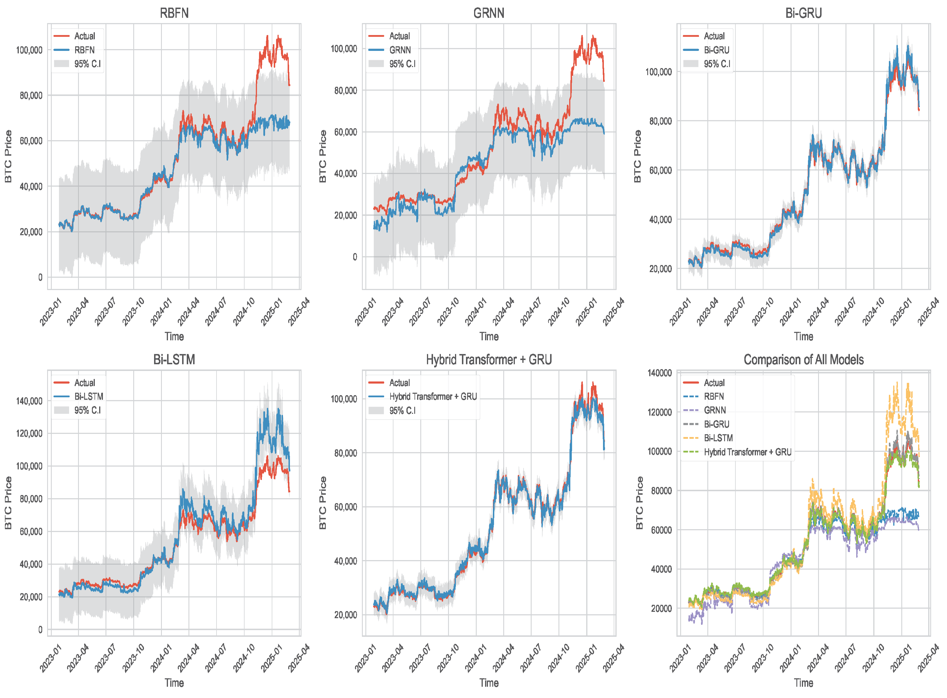
Model	MSE	RMSE	MAE	MAPE
RBFN	$1.731258\times {10}^8$	13157.727	6928.640	9.479%
GRNN	$1.875502\times {10}^8$	13694.897	9179.342	15.857%
BiGRU	$4.358457\times {10}^6$	2087.692	1559.954	3.271%
BiLSTM	$8.184621\times {10}^7$	9046.889	5877.042	9.600%
Hybrid Transformer + GRU	$3.818128\times {10}^6$	1954.003	1419.972	2.825%

and

Table 3. Performance metrics (MSE, RMSE, MAE, and MAPE) for predicting the prices of Ethereum using different models.

Model	MSE	RMSE	MAE	MAPE
RBFN	203,541.169	451.155	288.453	9.362%
GRNN	194,985.943	441.572	345.963	11.901%
BiGRU	687,799.984	829.337	608.416	20.735%
BiLSTM	907,844.180	952.809	675.427	22.640%
Hybrid Transformer + GRU	11,344.686	106.511	78.809	2.755%

present the comparison of performance metrics results for the proposed Hybrid Transformer + GRU network and the other four neural networks for predicting the prices of Bitcoin and Ethereum, respectively. From these two tables, it is seen that the proposed model is substantially superior, its compositors achieving more precise predictions as it always gives small prediction errors. For example, as shown in Table 2, when comparing the four compositor machine learning models, the BiGRU network achieves the smallest MSE value of $4,358,457$ for Bitcoin price prediction. Meanwhile, the MSE value for the proposed Hybrid Transformer + GRU model is $3,818,128$. For Ethereum price prediction, as shown in Table 3, the proposed model demonstrates excellent performance with an MSE of $11,344.686$. This is approximately 18 times smaller than the RBNF model’s MSE ($203,541.169$), 17 times smaller than GRNN’s ($194,985.943$), 60 times smaller than BiGRU’s ($687,799.984$), and 80 times smaller than BiLSTM’s ($907,844.180$). From the results in both tables, we can see that the feedforward neural networks (RBFN and GRNN) struggled to accurately predict Bitcoin prices. On the other hand, both bidirectional models (BiGRU and BiLSTM) did not perform as well when it came to predicting Ethereum prices.

The Friedman test results show a statistically significant difference in performance among the five Bitcoin price prediction models $({\chi }^2=1419.34$, p-value < 0.001), indicating that the models did not perform equally. As shown in

Table 4. Pairwise model comparisons for Bitcoin price prediction using Wilcoxon signed-rank test with Bonferroni correction. * indicates statistical significance at the level $\alpha =0.05$.

Model 1	Model 2	Wilcoxon Test	Raw p-Value	Bonferroni Corrected p-Value	Significant *
RBFN	GRNN	38,606	$1.78\times {10}^{-69}$	$1.78\times {10}^{-68}$	TRUE
RBFN	BiGRU	47,196	$4.23\times {10}^{-59}$	$4.23\times {10}^{-58}$	TRUE
RBFN	BiLSTM	132,787	0.02894864	0.2894864	FALSE
RBFN	Hybrid Transformer + GRU	34,773	$2.20\times {10}^{-74}$	$2.20\times {10}^{-73}$	TRUE
GRNN	BiGRU	5058	$3.17\times {10}^{-118}$	$3.17\times {10}^{-117}$	TRUE
GRNN	BiLSTM	47,851	$2.41\times {10}^{-58}$	$2.41\times {10}^{-57}$	TRUE
GRNN	Hybrid Transformer + GRU	2604	$2.64\times {10}^{-122}$	$2.64\times {10}^{-121}$	TRUE
BiGRU	BiLSTM	20,834	$1.14\times {10}^{-93}$	$1.14\times {10}^{-92}$	TRUE
BiGRU	Hybrid Transformer + GRU	128,651	0.004209894	0.042098938	FALSE
BiLSTM	Hybrid Transformer + GRU	21,898	$4.06\times {10}^{-92}$	$4.06\times {10}^{-91}$	TRUE

, post hoc pairwise comparisons using the Wilcoxon signed-rank test with Bonferroni correction revealed that the Hybrid Transformer + GRU model significantly outperformed RBFN, GRNN, and BiLSTM. However, its performance was not significantly better than that of the BiGRU model (p-value $=0.0421>{\alpha }^{*}=0.005)$. Additionally, BiGRU showed significantly stronger performance compared with both Bi-LSTM and GRNN, while RBFN was the weakest model overall, outperformed by all others except BiLSTM. Overall, both the BiGRU and the Hybrid Transformer + GRU models performed the best for Bitcoin price prediction, with only slight variations between them.

Similar to the Bitcoin results, the Friedman test shows significant performance differences among the five Ethereum prediction models $({\chi }^2=747.76$, p-value < 0.001). As shown in

Table 5. Pairwise model comparisons for Ethereum price prediction using Wilcoxon signed-rank test with Bonferroni correction. * indicates statistical significance at the level $\alpha =0.05$.

Model 1	Model 2	Wilcoxon Test	Raw p-Value	Bonferroni Corrected p-Value	Significant *
RBFN	GRNN	47,616	$2.49\times {10}^{-11}$	$2.49\times {10}^{-10}$	TRUE
RBFN	BiGRU	20,411	$2.19\times {10}^{-46}$	$2.19\times {10}^{-45}$	TRUE
RBFN	BiLSTM	15,193	$5.61\times {10}^{-56}$	$5.61\times {10}^{-55}$	TRUE
RBFN	Hybrid Transformer + GRU	17,810	$4.73\times {10}^{-51}$	$4.73\times {10}^{-50}$	TRUE
GRNN	BiGRU	29,575	$8.83\times {10}^{-32}$	$8.83\times {10}^{-31}$	TRUE
GRNN	BiLSTM	26,767	$5.93\times {10}^{-36}$	$5.93\times {10}^{-35}$	TRUE
GRNN	Hybrid Transformer + GRU	5615	$5.43\times {10}^{-76}$	$5.43\times {10}^{-75}$	TRUE
BiGRU	BiLSTM	46,690	$4.11\times {10}^{-12}$	$4.11\times {10}^{-11}$	TRUE
BiGRU	Hybrid Transformer + GRU	4900	$1.31\times {10}^{-77}$	$1.31\times {10}^{-76}$	TRUE
BiLSTM	Hybrid Transformer + GRU	4839	$9.48\times {10}^{-78}$	$9.48\times {10}^{-77}$	TRUE

, post hoc Wilcoxon signed-rank tests with Bonferroni correction showed that the Hybrid Transformer + GRU model significantly outperformed all other models, including BiGRU and BiLSTM. The results are consistent with the Bitcoin analysis, confirming the robustness of our proposed model across different digital cryptocurrencies.

5. Conclusions and Recommendation

The results obtained in this study show better performance of a novel attention-based Hybrid Transformer model in predicting cryptocurrency prices compared with two feedforward neural networks (radial basis function, RBFN, and general regression neural network, GRNN) and two deep learning models (bidirectional gated recurrent unit, BiGRU, and bidirectional long short-term memory, BiLSTM). Our proposed model builds on the same Transformer architecture, the foundation behind AI systems like ChatGPT and DeepSeek. The academic contribution of this study lies in demonstrating how a hybrid architecture that combines long-range pattern recognition with short-term temporal modeling can enhance time series forecasting. Practically, our model offers potential for improving real-time decision making in cryptocurrency markets, particularly for traders and analysts seeking data-driven strategies based on historical patterns. We conducted the comparison study using the two leading digital assets, Bitcoin and Ethereum, based on historical data with a one-time-step lag. When predicting Bitcoin prices, the proposed model achieves 6–7 times lower RMSE, 4–6 times lower MAE, and 3–6 times lower MAPE compared with the RBFN and GRNN models. For Ethereum, our model reduces RMSE by about 4 times, MAE by 3–4 times, and MAPE by 3–4 times compared with RBFN and GRNN. On the other hand, when we predict the Bitcoin prices, the proposed model achieves 1–5 times lower RMSE, 1–4 times lower MAE, and 1–3 times lower MAPE compared with the BiGRU and BiLSTM models. Moreover for Ethereum, our model reduces RMSE, MAE, and MAPE by approximately 8–9 times compared with the BiGRU and BiLSTM models. This study has certain limitations. First, it focuses only on Bitcoin and Ethereum, which, while dominant, do not represent the full spectrum of cryptocurrency behavior. Second, the model uses a fixed one-time-step lag, which may not capture more complex temporal dependencies. Third, we relied primarily on historical price, volume, and the Fear and Greed Index; other macroeconomic or blockchain-based indicators could further enrich the model. Future research could address these limitations by applying the model to a wider range of univariate and multivariate digital assets, as well as stock markets (e.g., as explored in Yan and Li [51]); testing different lag structures; and exploring alternative hybrid architectures such as Transformer + LSTM or Transformer + BiLSTM/BiGRU.

References

- Razi, M.A.; Athappilly, K. A comparative predictive analysis of neural networks (NNS), nonlinear regression and classification and regression tree (CART) models. Expert Syst. Appl. 2005, 29, 65–74. [Google Scholar] [CrossRef]
- Ślepaczuk, R.; Zenkova, M. Robustness of support vector machines in algorithmic trading on cryptocurrency market. Cent. Eur. Econ. J. 2018, 5, 186–205. [Google Scholar] [CrossRef]
- Chen, Z.; Li, C.; Sun, W. Bitcoin price prediction using machine learning: An approach to sample dimension engineering. J. Comput. Appl. Math. 2020, 365, 112395. [Google Scholar] [CrossRef]
- Mahdi, E.; Leiva, V.; Mara’Beh, S.; Martin-Barreiro, C. A New Approach to Predicting Cryptocurrency Returns Based on the Gold Prices with Support Vector Machines during the COVID-19 Pandemic Using Sensor-Related Data. Sensors 2021, 21, 6319. [Google Scholar] [CrossRef]
- Akyildirim, E.; Goncu, A.; Sensoy, A. Prediction of cryptocurrency returns using machine learning. Ann. Oper. Res. 2021, 297, 3–36. [Google Scholar] [CrossRef]
- Makala, D.; Li, Z. Prediction of gold price with ARIMA and SVM. J. Phys. Conf. Ser. 2021, 1767, 012022. [Google Scholar] [CrossRef]
- Jaquart, P.; K¨opke, S.; Weinhardt, C. Machine learning for cryptocurrency market prediction and trading. J. Financ. Data Sci. 2022, 8, 331–352. [Google Scholar] [CrossRef]
- Mahdi, E.; Al-Abdulla, A. Impact of COVID-19 Pandemic News on the Cryptocurrency Market and Gold Returns: A Quantile-on-Quantile Regression Analysis. Econometrics 2022, 10, 26. [Google Scholar] [CrossRef]
- Qureshi, M.; Iftikhar, H.; Rodrigues, P.C.; Rehman, M.Z.; Salar, S.A.A. Statistical Modeling to Improve Time Series Forecasting Using Machine Learning, Time Series, and Hybrid Models: A Case Study of Bitcoin Price Forecasting. Mathematics 2024, 12, 3666. [Google Scholar] [CrossRef]
- Broomhead, D.S.; Lowe, D. Radial Basis Functions, Multi-Variable Functional Interpolation and Adaptive Networks (Technical Report); Memorandum 4148; Royal Signals and Radar Establishment (RSRE): Malvern, UK, 1988. [Google Scholar]
- Broomhead, D.S.; Lowe, D. Multivariable functional interpolation and adaptive networks. Complex Syst. 1988, 2, 321–355. [Google Scholar]
- Alahmari, S.A. Predicting the Price of Cryptocurrency Using Support Vector Regression Methods. J. Mech. Contin. Math. Sci. 2020, 15, 313–322. [Google Scholar] [CrossRef]
- Casillo, M.; Lombardi, M.; Lorusso, A.; Marongiu, F.; Santaniello, D.; Valentino, C. Sentiment Analysis and Recurrent Radial Basis Function Network for Bitcoin Price Prediction. In Proceedings of the IEEE 21st Mediterranean Electrotechnical Conference (MELECON), Palermo, Italy, 14–16 June 2022; pp. 1189–1193. [Google Scholar] [CrossRef]
- Zhang, Y. Stock price behavior determination using an optimized radial basis function. Intell. Decis. Technol. 2025, 1–18. [Google Scholar] [CrossRef]
- Specht, D.F. A general regression neural network. IEEE Trans. Neural Netw. 1991, 2, 568–576. [Google Scholar] [CrossRef]
- Martínez, F.; Charte, F.; Rivera, A.J.; Frías, M.P. Automatic Time Series Forecasting with GRNN: A Comparison with Other Models. In Advances in Computational Intelligence, Proceedings of the 15th International Work-Conference on Artificial Neural Networks, IWANN 2019, Gran Canaria, Spain, 12–14 June 2019; Rojas, I., Joya, G., Catala, A., Eds.; Lecture Notes in Computer Science; Springer: Cham, Switzerland, 2019; p. 11506. [Google Scholar] [CrossRef]
- Martínez, F.; Charte, F.; Frías, M.P.; Martínez-Rodríguez, A.M. Strategies for time series forecasting with generalized regression neural networks. Neurocomputing 2022, 49, 509–521. [Google Scholar] [CrossRef]
- Hochreiter, S.; Schmidhuber, J. Long short-term memory. Neural Comput. 1997, 9, 1735–1780. [Google Scholar] [CrossRef]
- McNally, S.; Roche, J.; Caton, S. Predicting the Price of Bitcoin Using Machine Learning. In Proceedings of the 26th Euromicro International Conference on Parallel, Distributed and Network-based Processing (PDP), Cambridge, UK, 21–23 March 2018; pp. 339–343. Available online: https://api.semanticscholar.org/CorpusID:206505441 (accessed on 27 April 2025).
- Liu, Y.; Gong, C.; Yang, L.; Chen, Y. DSTP-RNN: A dual-stage two-phase attention-based recurrent neural network for long-term and multivariate time series prediction. Expert Syst. Appl. 2020, 143, 113082. [Google Scholar] [CrossRef]
- Zoumpekas, T. Houstis, E.; Vavalis, M. ETH analysis and predictions utilizing deep learning. Expert Syst. Appl. 2020, 162, 113866. [Google Scholar] [CrossRef]
- Lahmiri, S.; Bekiros, S. Cryptocurrency forecasting with deep learning chaotic neural networks. Chaos Solitons Fractals 2019, 118, 35–40. [Google Scholar] [CrossRef]
- Ji, S.; Kim, J.; Im, H. A Comparative Study of Bitcoin Price Prediction Using Deep Learning. Mathematics 2019, 7, 898. [Google Scholar] [CrossRef]
- Uras, N.; Marchesi, L.; Marchesi, M.; Tonelli, R. Forecasting Bitcoin closing price series using linear regression and neural networks models. PeerJ Comput. Sci. 2020, 6, E279. [Google Scholar] [CrossRef]
- Lahmiri, S.; Bekiros, S. Deep learning forecasting in cryptocurrency high frequency trading. Cogn. Comput. 2021, 13, 485–487. [Google Scholar] [CrossRef]
- Cho, K.; Merrienboer, B.; Gulcehre, C.; Bahdanau, D.; Fethi, B.; Holger, S.; Bengio, Y. Learning phrase representations using RNN encoder- decoder for statistical machine translation. arXiv 2014, arXiv:1406.1078. [Google Scholar]
- Jianwei, E.; Ye, J.; Jin, H. A novel hybrid model on the prediction of time series and its application for the gold price analysis and forecasting. Phys. A Stat. Mech. Its Appl. 2019, 527, 121454. [Google Scholar] [CrossRef]
- Dutta, A.; Kumar, S.; Basu, M. A gated recurrent unit approach to bitcoin price prediction. J. Risk Financ. Manag. 2020, 13, 23. [Google Scholar] [CrossRef]
- Tanwar, S.; Patel, N.P.; Patel, S.N.; Patel, J.R.; Sharma, G.; Davidson, I.E. Deep Learning-Based Cryptocurrency Price Prediction Scheme with Inter-Dependent Relations. IEEE Access 2021, 9, 138633–138646. [Google Scholar] [CrossRef]
- Ye, Z.; Wu, Y.; Chen, H.; Pan, Y.; Jiang, Q. A Stacking Ensemble Deep Learning Model for Bitcoin Price Prediction Using Twitter Comments on Bitcoin. Mathematics 2022, 10, 1307. [Google Scholar] [CrossRef]
- Patra, G.R.; Mohanty, M.N. Price Prediction of Cryptocurrency Using a Multi-Layer Gated Recurrent Unit Network with Multi Features. Comput. Econ. 2023, 62, 1525–1544. [Google Scholar] [CrossRef]
- Hansun, S.; Wicaksana, A.; Khaliq, A.Q.M. Multivariate cryptocurrency prediction: Comparative analysis of three recurrent neural networks approaches. J. Big Data 2022, 9, 50. [Google Scholar] [CrossRef]
- Ferdiansyah, F.; Othman, S.H.; Radzi, R.Z.M.; Stiawan, D.; Sutikno, T. Hybrid gated recurrent unit bidirectional-long short-term memory model to improve cryptocurrency prediction accuracy. IAES Int. J. Artif. Intell. (IJ-AI) 2023, 12, 251–261. [Google Scholar] [CrossRef]
- Vaswani, A.; Shazeer, N.; Parmar, N.; Uszkoreit, J.; Jones, L.; Gomez, A.N.; Polosukhin, I. Attention is all you need. Adv. Neural Inf. Process. Syst. 2017, 30, 5998–6008. [Google Scholar]
- Devlin, J.; Chang, M.W.; Lee, K.; Toutanova, K. BERT: Pre-training of deep bidirectional transformers for language understanding. In Proceedings of the 2019 Conference of the North American Chapter of the Association for Computational Linguistics: Human Language Technologies, Volume 1 (Long and Short Papers), Minneapolis, MN, USA, 2–7 June 2019; pp. 4171–4186. [Google Scholar] [CrossRef]
- Dosovitskiy, A.; Beyer, L.; Kolesnikov, A.; Weissenborn, D.; Zhai, X.; Unterthiner, T.; Dehghani, M.; Minderer, M.; Heigold, G.; Gelly, S.; et al. An Image is Worth 16 × 16 Words: Transformers for Image Recognition at Scale. arXiv 2020, arXiv:2010.11929. [Google Scholar]
- Zhou, H.; Zhang, S.; Peng, J.; Zhang, S.; Li, J.; Xiong, H.; Zhang, W. Informer: Beyond Efficient Transformer for Long Sequence Time-Series Forecasting. Proc. AAAI Conf. Artif. Intell. 2021, 35, 11106–11115. [Google Scholar] [CrossRef]
- Grigsby, J.; Wang, Z.; Qi, Y. Long-Range Transformers for Dynamic Spatiotemporal Forecasting. arXiv 2021, arXiv:2109.12218. [Google Scholar]
- Lezmi, E.; Xu, J. Time Series Forecasting with Transformer Models and Application to Asset Management. 2023. Available online: https://ssrn.com/abstract=4375798 (accessed on 27 April 2025).
- Wen, Q.; Zhou, T.; Zhang, C.; Chen, W.; Ma, Z.; Yan, J.; Sun, L. Transformers in Time Series: A Survey. In Proceedings of the Thirty-Second International Joint Conference on Artificial Intelligence, IJCAI-23, Macao, 19–25 August 2023; pp. 6778–6786. [Google Scholar] [CrossRef]
- Li, S.; Jin, X.; Xuan, Y.; Zhou, X.; Chen, W.; Wang, Y.X.; Yan, X. Enhancing the locality and breaking the memory bottleneck of transformer on time series forecasting. arXiv 2020, arXiv:1907.00235. [Google Scholar]
- Zerveas, G.; Jayaraman, S.; Patel, D.; Bhamidipaty, A.; Eickhoff, C. A transformer-based framework for multivariate time series representation learning. In Proceedings of the KDD ’21: Proceedings of the 27th ACM SIGKDD Conference on Knowledge Discovery & Data Mining, Virtual Event, Singapore, 14–18 August 2021; pp. 2114–2124. [Google Scholar] [CrossRef]
- Wu, H.; Xu, J.; Wang, J.; Long, M. Autoformer: Decomposition transformers with auto-correlation for long-term series forecasting. NeurIPS. arXiv 2021, arXiv:2106.13008. [Google Scholar]
- Castangia, M.; Grajales, L.M.M.; Aliberti, A.; Rossi, C.; Macii, A.; Macii, E.; Patti, E. Transformer neural networks for interpretable flood forecasting. Environ. Model. Softw. 2023, 160, 105581. [Google Scholar] [CrossRef]
- Nayak, G.H.H.; Alam, W.; Avinash, G.; Kumar, R.R.; Ray, M.; Barman, S.; Singh, K.N.; Naik, B.S.; Alam, N.M.; Pal, P.; et al. Transformer-based deep learning architecture for time series forecasting. Softw. Impacts 2024, 22, 100716. [Google Scholar] [CrossRef]
- Kristoufek, L. BitCoin meets Google Trends and Wikipedia: Quantifying the relationship between phenomena of the Internet era. Sci. Rep. 2013, 3, 3415. [Google Scholar] [CrossRef]
- Urquhart, A. What causes the attention of Bitcoin? Econ. Lett. 2018, 166, 40–44. [Google Scholar] [CrossRef]
- Kao, Y.S.; Day, M.Y.; Chou, K.H. A comparison of bitcoin futures return and return volatility based on news sentiment contemporaneously or lead-lag. N. Am. J. Econ. Financ. 2024, 72, 102159. [Google Scholar] [CrossRef]
- Mai, F.; Shan, J.; Bai, Q.; Sahne, W. How does social media impact Bitcoin value? A test of the silent majority hypothesis. J. Manag. Inf. Syst. 2018, 35, 19–52. [Google Scholar] [CrossRef]
- Garcia, D.; Schweitzer, F. Social signals and algorithmic trading of Bitcoin. R. Soc. Open Sci. 2015, 2, 150288. [Google Scholar] [CrossRef]
- Yan, K.; Li, Y. Machine learning-based analysis of volatility quantitative investment strategies for American financial stocks. Quant. Financ. Econ. 2024, 8, 364–386. [Google Scholar] [CrossRef]