OWNC: Open-World Node Classification on Graphs with a Dual-Embedding Interaction Framework

Abstract

Traditional node classification is typically conducted in a closed-world setting, where all labels are known during training, enabling graph neural network methods to achieve high performance. However, in real-world scenarios, the constant emergence of new categories and updates to existing labels can result in some nodes no longer fitting into any known category, rendering closed-world classification methods inadequate. Thus, open-world classification becomes essential for graph data. Due to the inherent diversity of graph data in the open-world setting, it is common for the number of nodes with different labels to be imbalanced, yet current models are ineffective at handling such imbalance. Additionally, when there are too many or too few nodes from unseen classes, classification performance typically declines. Motivated by these observations, we propose a solution to address the challenges of open-world node classification and introduce a model named OWNC. This model incorporates a dual-embedding interaction training framework and a generator–discriminator architecture. The dual-embedding interaction training framework reduces label loss and enhances the distinction between known and unseen samples, while the generator–discriminator structure enhances the model’s ability to identify nodes from unseen classes. Experimental results on three benchmark datasets demonstrate the superior performance of our model compared to various baseline algorithms, while ablation studies validate the underlying mechanisms and robustness of our approach.

1. Introduction

In recent years, the rapid development of Graph Neural Networks (GNNs) has led to significant progress in graph learning. As a classic task in graph learning, node classification attempts to classify nodes in a graph into several groups, assigning labels (categories) to unlabeled nodes. This task has numerous important applications, including social network analysis [1], knowledge graphs [2], fraud detection [3], protein–protein interaction prediction [4], recommendation systems [5], and chemical compound classification [6].

Existing node classification methods [7,8,9] primarily learn in a “closed-world” setting, meaning that the nodes in the test data must be assigned to one or more categories that have been seen in the training set [10]. Therefore, if nodes belonging to a new or unseen category appear in the test set, the classifier cannot detect these new or unseen categories and will incorrectly classify these nodes into categories already seen in the training data. Take a social media platform as an example. We may apply a trained graph neural network to a social media platform to identify emerging topics or communities. However, when new interests or trends emerge among users, the neural network will naturally fail to classify these latest trends and cannot adjust recommendations or advertising strategies accordingly. This limits the effectiveness of GNNs in real-world applications.

To address this issue, the task called “open-world” classification [11], which aims to learn and recognize previously seen categories and simultaneously detect new category samples (as shown in Figure 1), was introduced to graph learning and has received increasing attention. Several previous studies have attempted to perform open-world classification. OpenWGL [12] rejects nodes that do not belong to a known class by automatically setting a threshold, marking those that do not meet the criteria as unknown class nodes, and ${\mathcal{G}}^{2}Pxy$ [13] predicts the distribution of unknown categories by generating mixed proxy nodes. However, these approaches often exhibit a high degree of fragility as even slight modifications to the task setup can lead to a significant drop in model performance. Specifically, when the model encounters multiple unseen categories simultaneously, the boundaries between classes in the feature space become increasingly blurred, making it challenging for the model to accurately distinguish between previously seen and new categories. Similarly, the presence of imbalanced known node samples can cause the model to skew toward more prevalent classes, thereby undermining its ability to correctly identify and classify nodes from less represented or new classes [14]. Such sensitivity to task configurations limits the reliability of these methods in practical scenarios, where data distributions and class appearances are often unpredictable and dynamic. Therefore, achieving effective open-world node classification requires not only the capacity to recognize nodes from unseen classes, but also the ability to improve the model’s practicality and robustness.

Figure 1. Given a graph with both labeled and unlabeled nodes (left panel), the goal of open-world graph learning is to train a classifier that not only categorizes unlabeled nodes from seen classes into their respective categories, but also identifies nodes that do not belong to any of the seen classes as unseen class nodes.

Motivated by these observations, we address the following challenges in dealing with open-world node classification.

• Imbalanced learning: It is common for the number of nodes with different labels to be imbalanced in the open-world setting due to the inherent diversity of the data. However, current models are ineffective in dealing with such imbalanced data.
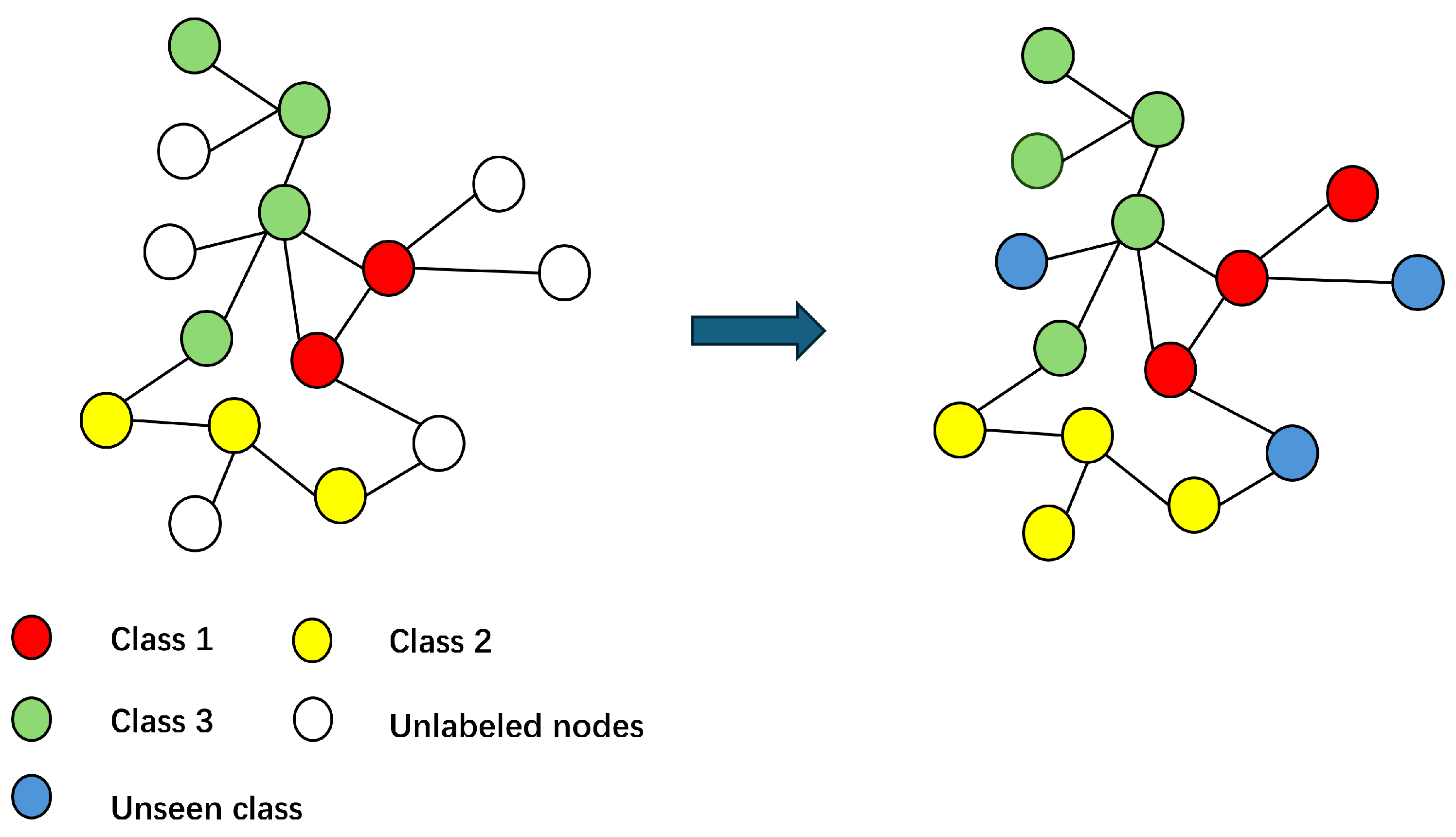
• Too many or too few nodes from unseen classes: When dealing with too many or too few nodes from the unseen classes, the classification is usually less effective.

To address the first challenge of imbalanced learning, we developed a dual-embedding interaction training framework to enhance the classification performance of nodes from seen classes. Imbalanced data often lead to poor performance on under-represented classes, making it challenging for models to generalize effectively in the open-world classification setting. Our framework incorporates two neural networks, each independently outputting predicted class probabilities. Moreover, the networks select and share low-loss samples with one another, allowing for mutual updating based on these low-loss samples. This sample-sharing mechanism enables the model to learn data features from multiple perspectives, which helps it handle hard-to-learn samples that are common in open-world settings due to the complex characteristics of minority classes. By maintaining two networks, our framework promotes diverse perspectives and reduces overfitting to specific samples. Particularly in an open-world learning scenario, this strategy enhances the model’s adaptability to data variability, supporting more robust and flexible classification outcomes.

For the second challenge, we employed a Generative Adversarial Network (GAN) to learn from nodes of unseen classes, and a generator–discriminator architecture was used to handle the classification of these nodes. When the number of nodes from unseen classes is small, GAN can effectively alleviate the problem by generating synthetic data, enhancing the model’s generalization capabilities on unseen classes. On the other hand, when faced with a large number of nodes from the unseen classes, our dual-embedding interaction training framework ensures the model remains stable under complex feature distributions. Additionally, GAN can help mitigate class imbalance within the dataset, improving the model performance in classifying minority classes and significantly enhancing the robustness of the model.

In summary, this paper proposes an open-world node classification framework for graph learning, called OWNC. Our approach addresses two major challenges in learning from diverse and complex graph data within an open-world setting: effectively handling imbalanced learning, and improving classification for varying numbers of nodes from unseen classes. Our dual-embedding interaction training framework enhances the learning process by maintaining two networks that select low-loss samples for each other. This approach helps manage hard-to-learn samples, maintain model compatibility, and prevent overfitting. Additionally, we employed a generator–discriminator architecture to generate synthetic features for nodes from unseen classes, alleviating issues related to imbalanced learning and enhancing the model’s generalization and robustness across complex feature distributions. Together, these components provide a comprehensive solution for open-world node classification, improving the adaptability and stability of graph learning models.

Based on these methods, our main contributions are summarized as follows.

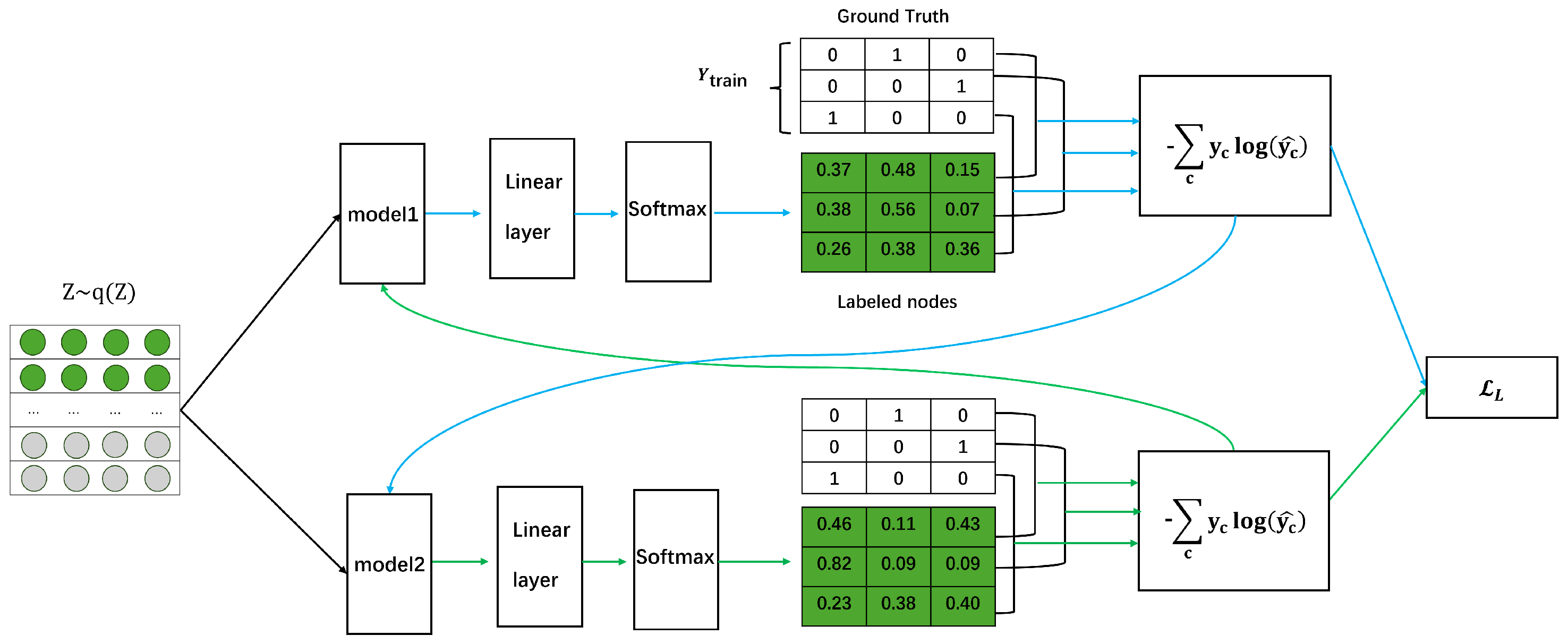
• We introduce a dual-embedding interaction training framework that enhances classification by effectively managing hard-to-learn samples, promoting model diversity through mutual sample selection, and reducing overfitting. These features collectively improve the model’s robustness and generalization, particularly in complex open-world scenarios.
• By integrating a GAN-based generator–discriminator architecture, our model maintains sensitivity to unseen classes, delivering strong performance regardless of whether there is a small or large number of nodes from unseen classes. This setup also mitigates imbalanced learning, further supporting the model’s ability to generalize.
• Our algorithm achieves significant performance improvements over state-of-the-art methods across three benchmark datasets, demonstrating its effectiveness in handling open-world node classification challenges.

2. Related Work

2.1. Open-World Learning

Open-world learning aims to recognize categories that the learner has previously seen or learned while detecting new categories that it has never encountered before. In recent years, this topic has garnered widespread attention. Bendale et al. introduced the concept of open-world recognition in 2015 [15], emphasizing that models not only need to classify known categories, but also need to identify samples from unknown categories.

Xian et al. [16] proposed a method that utilizes knowledge of known categories to infer samples of unknown categories through shared attributes or semantic information. This approach is significant in handling large-scale datasets and open-world problems.

Wu et al. [12] trained a variational graph autoencoder to learn embeddings, optimizing it to increase the model’s uncertainty for new categories and refusing to classify nodes with high uncertainty in predictions. However, the classification performance is poor when the model faces a large number of unseen node categories.

Zhang et al. [13] proposed a generative open-set node classification method based on proxy unknown nodes. Although this method progressed in certain aspects, it performed poorly in handling multiple unseen categories, failing to achieve good classification results.

However, these existing methods still struggle to handle multiple unseen categories and maintain robust classification performance in complex, high-dimensional open-world scenarios. Additionally, they often experience performance degradation when faced with a large number of unknown categories, highlighting an urgent need for more flexible and scalable solutions in open-world learning.

2.2. Graph Neural Networks

In the task of node classification, Graph Neural Networks (GNNs) have become a highly active area of research. Kipf and Welling proposed Graph Convolutional Networks (GCNs) [7], a model based on spectral graph theory for semi-supervised learning on graph-structured data. GCNs combine node feature information and structural information through a local neighborhood aggregation operation, thereby enabling node classification tasks.

Hamilton et al. [9] proposed GraphSAGE (Graph Sample and Aggregation), a graph neural network that can efficiently operate on large-scale graphs. GraphSAGE reduces computational complexity by randomly sampling neighboring nodes and aggregating their features, and it can perform node classification in an inductive setting.

Velickovic et al. introduced Graph Attention Networks (GATs) [8], which incorporate an attention mechanism, allowing the model to adaptively assign different neighbor weights for each node. GATs, through multi-head attention mechanisms, can better capture the complex relationships between nodes.

While traditional neural networks have demonstrated strong performance in closed-world settings, they often fall short in open-world scenarios [17]. These conventional methods are typically designed with the assumption that all categories are known during training, limiting their ability to handle unseen categories or to adapt to novel, complex structures. As a result, their effectiveness diminishes in open-world tasks, where models must not only classify known categories, but also detect and adapt to new or unknown classes.

2.3. Co-Training Related Methods

In supervised learning, neural networks often tend to fit easily learnable data first. Taking advantage of this, MentorNet introduces a pre-trained network to select clean samples, guiding the training of the main model [18]. However, when clean validation data are unavailable, MentorNet relies on predefined curricula [19]. Although this self-paced selection is similar to self-training methods, it also inherits the cumulative error problem caused by sample selection bias in self-training [20].

Decoupling [21], on the other hand, avoids bias by simultaneously training two networks and only updating the model when these two networks make different predictions on the same instance.

Blum et al. introduced the co-training algorithm, a foundational semi-supervised learning approach that leverages both labeled and unlabeled data by training two classifiers on different feature views of the data, allowing them to iteratively teach each other to improve classification performance [22].

Han et al. proposed the co-teaching training method [23]. During training, two neural networks are maintained independently, each updating its parameters separately. In each batch of training data, the two networks independently select samples with the smallest loss and pass these samples to each other for training. The proportion of small-loss samples selected increases gradually during training, further reducing overall loss. Through this collaborative training approach, the co-teaching method effectively improves model performance.

Yu et al. proposed the co-teaching+ method [24]. Unlike the co-teaching method, co-teaching+ does not rely solely on selecting low-loss samples from two networks. Instead, it guides the training process through the consistency between the two networks. Specifically, when selecting samples, co-teaching+ not only focuses on low-loss samples, but it also requires that the two networks make consistent predictions on the same sample. Only when both networks make the same prediction is the sample used to update the model parameters.

However, in an open-world environment, a major challenge for these methods is their difficulty in effectively handling data from unknown categories. Since these methods typically rely on low-loss samples from known categories or consistency judgments to guide training, they may exhibit bias when encountering entirely unknown categories.

2.4. Generator and Discriminator

Generative Adversarial Networks (GANs), first proposed by Ian Goodfellow et al. in 2014 [25], consist of two neural networks: a generator and a discriminator. Mirza and Osindero later introduced Conditional GANs (cGANs), which extend this framework by allowing sample generation conditioned on specific class labels, thus enabling the model to generate data for particular categories [26]. These networks are trained through an adversarial process, ultimately generating high-quality data samples.

The generator receives random noise as input and attempts to generate realistic data samples that closely resemble the distribution of real data. The discriminator acts as a judge, determining whether the input data is real or generated by the generator [27]. The two networks are trained in an adversarial manner: the generator tries to deceive the discriminator into believing the generated data are real, while the discriminator continually improves its ability to distinguish between real and fake data accurately. This adversarial training process iterates until the generator produces data so realistic that the discriminator can no longer effectively distinguish between real and generated data. Through this iterative process, the generator gradually learns to capture the features of real data, resulting in increasingly higher-quality samples. GANs have been successfully applied in various fields, such as image synthesis, text-to-image generation, and data augmentation [28].

In open-world datasets, obtaining features for unseen class samples is challenging, often limiting a model’s ability to learn from unknown categories [29]. GANs, by generating samples of unseen classes, expand the model’s capacity to learn features of unknown categories. This approach not only enhances the model’s generalization capability, but also addresses the problem of data scarcity in open-world scenarios, enabling more robust performance in the face of unseen classes [30].

Although GANs can simulate samples of unseen classes through the generator to help the model expand its ability to learn features of unknown categories, the quality and diversity of generated samples may be limited. Specifically, the GAN generator may fail to accurately capture the complex features of all unknown categories, resulting in samples that do not fully represent real unseen category data. Additionally, since the generator relies on the distribution of known data to learn features, it may produce inaccurate samples or deviate from the true distribution in an open-world setting, which can affect the model’s generalization capability. Such inaccurately generated samples may introduce noise to the classification model, leading to misclassifications or biased judgments of unknown categories.

3. Problem Definition and Framework Structure

3.1. Problem Definition

This paper focused on the node classification problem. We define a graph $G=(V,E,X,Y)$, in which $V={\left\{v_i\right\}}_{i=1,\dots ,N}$ is a set of N nodes; $E=\left\{e_{i,j}\right\}$ is the set of edges; i and j range from 1 to N; and $i\ne j$ represent the connection between the node pair $(v_i,v_j)$. The label matrix is $Y\in {\mathbb{R}}^{N\times C}$, where N is the total number of nodes and C is the number of known classes. If node i has label l, then $Y_{\left(i\right)}^l=1$; otherwise, $Y_{\left(i\right)}^l=0$.

The adjacency matrix A is used to represent the topological structure of graph G, where $A_{i,j}=1$ if $(v_i,v_j)\in E$, and $A_{i,j}=0$ otherwise. The content feature representation of each node $v_i\in V$ is given by $x_i\in X$, representing its features.

In an open-world learning scenario, for graph $G=(V,E,X,Y)$, we have $X=X_{\mathrm{train}}\cup X_{\mathrm{test}}$; $X_{\mathrm{train}}$ is the labeled nodes for training; and $X_{\mathrm{test}}$ is the unlabeled testing nodes. In addition, $X_{\mathrm{test}}$ can be divided into two sets: S and U. Here, S consists of nodes belonging to categories that have already appeared in $X_{\mathrm{train}}$, and U consists of nodes that do not belong to any known category (i.e., unseen category nodes). The goal of open-world graph learning is to train a $(C+1)$-class classifier model f that can map each test node $X_{\mathrm{test}}$ to a label set Y, i.e., $f\left(X_{\mathrm{test}}\right)\to Y$, where $Y\in \{1,\dots ,C,\mathrm{reject}\}$. This model needs to classify test nodes S into known training categories and reject U nodes, indicating that they belong to unseen categories and do not belong to any category in the training set.

3.2. Framework Structure

Our model consists of three parts, as shown in Figure 2.

Figure 2. Overall Framework. This figure illustrates the process for open-world node classification. It demonstrates the complete workflow, starting from the input graph data, which is processed through a graph convolutional encoder; followed by latent representation learning via an autoencoder (AE); and, finally, reconstruction and node label prediction is delivered through a decoder. The model integrates both graph structure and node features, aiming to enhance classification performance for unlabeled nodes.

The first part is a graph autoencoder model used to generate deterministic mappings to capture the latent features and distribution of the nodes, thereby representing uncertainty. We denote the loss of this part as ${\mathcal{L}}_{\mathrm{AE}}$. For more details, see Section 4. Additionally, in the following Part 2 and Part 3, we will provide a detailed explanation of the label loss and unlabeled loss.

The second part is the open-world labeled loss. Two models are used to improve classification performance through a training framework. Both models receive the input node features and output class probability distributions, respectively. Each model selects its own low-loss samples to pass to the other model for training. The information flow shown in the figure illustrates the process of sample passing, enhancing the robustness of the classification. This was illustrated to better classify the known nodes, as shown in Figure 3.

Figure 3. Open-world known node classification process. This was constructed to better classify the known nodes, which are shown in Figure 3. For more detailed information, see the labeled loss function in Section 4.

The third part is the ppen-world unlabeled loss. For unlabeled loss, we introduced a generator and a discriminator to help the model better identify unseen nodes. The generator is responsible for generating embeddings of unlabeled nodes, while the discriminator evaluates the authenticity of these embeddings. In this way, we can enhance the model’s ability to recognize unknown categories and improve the overall classification performance. An illustration of this open-world unseen node classification process is shown in Figure 4. For more detailed information, see the unlabeled loss function in Section 4.

Figure 4. Open-world unseen node classification. Through using GAN for data augmentation, we aim to deliver exceptional performance in identifying unseen nodes.

4. Framework Structure

4.1. Open-World Classifier Learning

To effectively train an accurate classifier capable of categorizing both known nodes and nodes from unseen classes in the test graph data, our proposed model includes a collaborative module with an autoencoder reconstruction loss (${\mathcal{L}}_{\mathrm{AE}}$), a labeled loss (${\mathcal{L}}_{\mathrm{L}}$), and an unlabeled loss (${\mathcal{L}}_{\mathrm{U}}$) from the three parts of the model, respectively. These components work together to differentiate whether a node belongs to an existing category or an unknown category. The overall objective function is as follows:

$$\begin{array}{c}\hfill \mathcal{L}={\mathcal{L}}_{\mathrm{AE}}+{\gamma }_1{\mathcal{L}}_{\mathrm{L}}+{\gamma }_2{\mathcal{L}}_{\mathrm{U}},\end{array}$$

(1)

where ${\gamma }_1$ and ${\gamma }_2$ are hyper-parameters to balance the losses. We introduce each of these modules in the following sections.

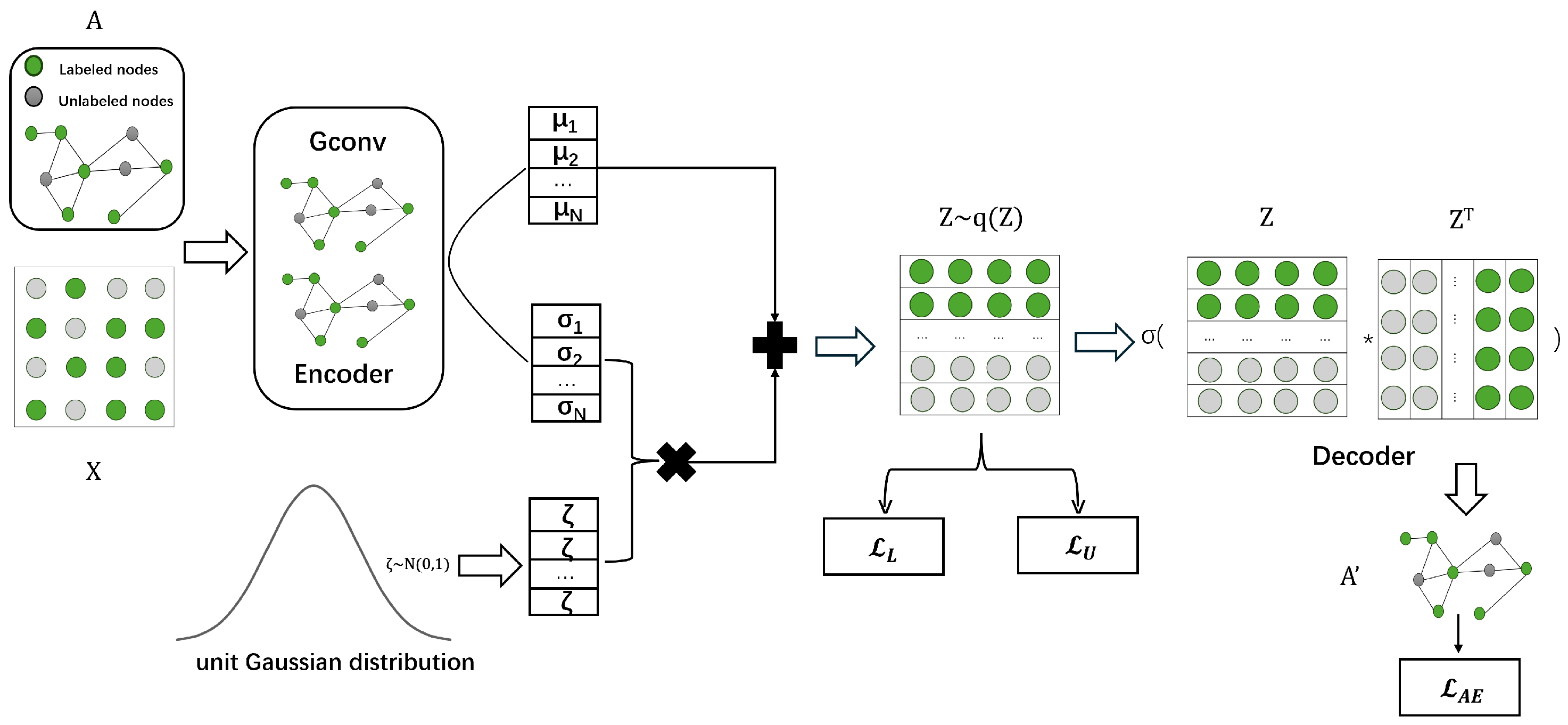
4.2. Graph Autoencoder Model

Graph Encoder: Given a graph $G=(X,A)$ with input feature matrix X and adjacency matrix A, we first follow [7] and employ a two-layer GCN to learn a unified low-dimensional feature matrix. The first layer is defined as follows:

$$\begin{array}{c}\hfill Z^{\left(1\right)}=\mathrm{GCN}(X,A)=\mathrm{ReLU}\left({\tilde{D}}^{-{\displaystyle \frac{1}{2}}}\tilde{A}{\tilde{D}}^{-{\displaystyle \frac{1}{2}}}X{W}^{\left(1\right)}\right),\end{array}$$

(2)

where ReLU is the activation function used to introduce non-linearity, $\tilde{A}=A+I_m$ is the adjacency matrix with self-loops, and $I_m$ is the identity matrix. The degree matrix $\tilde{D}$ is defined as ${\tilde{D}}_{i,i}={\sum }_j{\tilde{A}}_{i,j}$. $\tilde{D}$ is to normalize the adjacency matrix, balance the influence of nodes with different degrees, and ensure stability and consistency in the information propagation within the graph convolutional network. $W^{\left(1\right)}$ is the trainable weight matrix.

For the second layer, we assume the output Z is continuous and follows a multivariate Gaussian distribution. An inference model [31] is adopted as follows:

$$\begin{array}{c}\hfill q(Z\mid X,A)=\prod _{i=1}^{M}q(z_i\mid X,A),\end{array}$$

(3)

$$\begin{array}{c}\hfill q(z_i\mid X,A)=\mathcal{N}(z_i\mid {\mu }_i,\mathrm{diag}\left({\sigma }_i^2\right)).\end{array}$$

(4)

Here, the mean vector matrix $\mu$ is defined as $\mu =\mathrm{ReLU}({\tilde{D}}^{-{\displaystyle \frac{1}{2}}}\tilde{A}{\tilde{D}}^{-{\displaystyle \frac{1}{2}}}{Z}^{\left(1\right)}{W}^{\left(2\right)})$. The standard deviation matrix $\sigma$ is defined as $\log \sigma =\mathrm{ReLU}({\tilde{D}}^{-{\displaystyle \frac{1}{2}}}\tilde{A}{\tilde{D}}^{-{\displaystyle \frac{1}{2}}}{Z}^{\left(1\right)}{W}^{\prime \left(2\right)})$, and $W^{\left(2\right)}$ and $W^{\prime \left(2\right)}$ are trainable weight matrices for the second GCN layer.

The latent representation Z can be computed using a reparameterization trick:

$$\begin{array}{c}\hfill Z=\mu +\sigma ·\xi ,\xi \sim \mathcal{N}(0,I),\end{array}$$

(5)

where $\xi$ is a noise vector sampled from a standard normal distribution with mean 0 and variance I.

Inner-product Decoder: After obtaining the latent variable Z, a decoder is employed to reconstruct the graph structure A from the latent variable Z. The graph decoding model is given by the generative model in [7]:

$$\begin{array}{c}\hfill p(A\mid Z)=\prod _{i=1}^N\prod _{j=1}^{N}p(A_{i,j}\mid z_i,z_j),\end{array}$$

(6)

$$\begin{array}{c}\hfill p(A_{ij}=1\mid {\mathbf{z}}_i,{\mathbf{z}}_j)=\sigma \left({\mathbf{z}}_i^T{\mathbf{z}}_j\right).\end{array}$$

(7)

Here, $A_{i,j}$ is an element of A; $p(A_{i,j}\mid {\mathbf{z}}_i,{\mathbf{z}}_j)$ is the probability of an edge existing between node i and node j, given the latent representations ${\mathbf{z}}_i$ and ${\mathbf{z}}_j$ of nodes i and j, respectively; $\sigma (·)$ represents the logistic sigmoid function; and ${\mathbf{z}}_i^{\top }{\mathbf{z}}_j$ is the inner product of the latent representation vectors of node i and node j.

Optimization: To better learn node representations with category discriminative power, we optimized the variational graph autoencoder (AE) module through the following loss:

$$\begin{array}{c}\hfill {\mathcal{L}}_{\mathrm{AE}}={\mathbb{E}}_{q(Z\mid X,A)}\left[\log p(A\mid Z)\right]-\mathrm{KL}\left[q(Z\mid X,A) \Vert p\left(Z\right)\right].\end{array}$$

(8)

The first term is the reconstruction loss between the input adjacency matrix and the reconstructed adjacency matrix. The second term is the Kullback–Leibler (KL) divergence:

$$\begin{array}{c}\hfill \mathrm{KL}\left[q(Z\mid X,A) \Vert p\left(Z\right)\right].\end{array}$$

(9)

where $p\left(Z\right)=\mathcal{N}(0,I)$.

By optimizing this loss term, we can better capture the complex relationships between the graph structure and node content. The KL divergence term constrains the latent space, encouraging the learned node representations Z to align with a standard normal distribution $\mathcal{N}(0,I)$, which helps prevent overfitting and improves generalization to unseen nodes.

4.3. Labeled Loss Function

The labeled loss function aims to minimize the cross-entropy loss of labeled data, and the basic formula could be formed as follows:

$$\begin{array}{c}\hfill {\mathcal{L}}_{\mathrm{L}}(f_s\left(Z_{\mathrm{labeled}}\right),Y)=-{\displaystyle \frac{1}{N_l}}\sum _{i=1}^{N_l}\sum _{c=1}^C(y_{i,c}\log ({\widehat{y}}_{i,c})).\end{array}$$

(10)

where $\mathcal{Y}$ refers to the ground truth label matrix; $N_l$ represents the number of labeled data; C is the number of known categories; $y_{i,c}$ represents the true label of the i-th sample belonging to class c; ${\widehat{y}}_{i,c}$ represents the predicted probability of the i-th sample belonging to class c; and $f_s(·)$ is a softmax layer containing fully connected layers with corresponding activation functions, which can convert $Z_{\mathrm{unlabeled}}$ into probabilities that sum to one.

Dual-embedding model loss: The dual-embedding interaction training framework aims to minimize the cross-entropy loss of labeled data via using two models to teach, selecting samples with the smallest loss from each other for training. Therefore, in the training framework, we have two models, $f_1$ and $f_2$, with their respective label losses. By selecting samples with the smallest loss from each model for training, we obtain the joint model loss:

$$\begin{array}{c}\hfill {\mathcal{L}}_{\mathrm{L}}(f_s\left(Z_{\mathrm{labeled}}\right),Y)=-{\displaystyle \frac{1}{2N_l}}\sum _{i=1}^{N_l}\sum _{c=1}^C(y_{i,c}\log ({\widehat{y}}_{1,i,c})\hfill \\ \hfill +y_{i,c}\log ({\widehat{y}}_{2,i,c})),\hfill \end{array}$$

(11)

where ${\widehat{y}}_{1,i,c}$ is the predicted probability from the first model that the i-th sample belongs to class c, and ${\widehat{y}}_{2,i,c}$ is the predicted probability from the second model that the i-th sample belongs to class c.

4.4. Unlabeled Loss

Class Uncertainty Loss: Since the test data lack class information and contain numerous nodes from unseen classes, we need to find a method to distinguish between known and unknown categories. Unlike ${\mathcal{L}}_{\mathrm{L}}$, which leverages abundant training data and performs well on known categories, the class uncertainty loss is proposed to balance the classification output for each node and perform well on unknown nodes. In our paper, entropy loss is used as the class uncertainty loss, denoted as ${\mathcal{L}}_{\mathrm{C}}$, and our goal is to maximize this entropy loss to make the normalized output of each node more balanced. The formula is as follows:

$$\begin{array}{c}\hfill {\mathcal{L}}_C\left(f_s\left(Z_{\mathrm{unlabeled}}\right)\right)={\displaystyle \frac{1}{N_u}}\sum _{i=1}^{N_u}\sum _{c=1}^C{\widehat{y}}_{i,c}\log \left({\widehat{y}}_{i,c}\right).\end{array}$$

(12)

Here, $N_u$ is the number of unlabeled nodes, and $y_i$ is the classification prediction score of the i-th unlabeled node $v_i$ for class c. Note that we do not add a negative sign in front of the formula as usual because we need to maximize the entropy loss. Furthermore, we do not use all of the unlabeled data to maximize the entropy loss. We first sort the output probability values of all unlabeled data after the softmax layer (selecting the maximum probability for each node), then discard the top 10% (nodes with high probability values are easily classified into known categories as their outputs are discriminative) and the bottom 10% of nodes (low probabilities mean the node’s output is balanced across each known category, and these nodes are also easily detected as unknown categories). Finally, we use the remaining nodes to maximize their entropy.

GAN Loss Function: Our GAN loss function is designed to optimize both the generator and discriminator to effectively model diverse feature characteristics.

$$\begin{array}{c}\hfill \mathrm{GAN}={\mathcal{L}}_{\mathrm{gen}}+{\mathcal{L}}_{\mathrm{disc}}.\end{array}$$

(13)

After obtaining the classification results of the unseen nodes, we can use the generator and discriminator to provide additional sample data to help train the model.

The goal of the generator is to deceive the discriminator into believing that the generated fake samples are real samples. To enhance the training effectiveness and robustness of the model, we aim to maximize the discriminator’s prediction value for the fake samples. Specifically, the generator loss function can be expressed as follows:

$$\begin{array}{c}\hfill {\mathcal{L}}_{\mathrm{gen}}={\mathbb{E}}_{z\sim p_z\left(z\right)}\left[\log \left(D\right(G\left(z\right)\left)\right)\right].\end{array}$$

(14)

In the open-world setting, we use cross-entropy loss to calculate the generator loss:

$$\begin{array}{c}\hfill {\mathcal{L}}_{\mathrm{gen}}={\mathbb{E}}_{z\sim p_z\left(z\right)}\left[\log \left(D\right(G\left(z\right)\left)\right)\right]=\mathrm{BCE}(1,D\left(G\left(z\right)\right)),\end{array}$$

(15)

where $G\left(z\right)$ is the fake sample generated by the generator, $D\left(G\right(z\left)\right)$ is the discriminator’s prediction for the generated fake sample, and BCE is the binary cross-entropy loss function.

The goal of the discriminator is to distinguish between real samples and fake samples. Specifically, the discriminator loss function consists of two parts: one part is the loss for the discriminator on the real samples, and the other part is the loss for the discriminator on the fake samples. The discriminator loss function can be expressed as follows:

$$\begin{array}{c}\hfill {\mathcal{L}}_{\mathrm{disc}}={\mathbb{E}}_{x\sim p_{\mathrm{data}}\left(x\right)}\left[\log \left(D\right(x\left)\right)\right]+{\mathbb{E}}_{z\sim p_z\left(z\right)}\left[\log (1-D(G\left(z\right)\left)\right)\right],\end{array}$$

(16)

where x is the real sample, and $D\left(x\right)$ is the discriminator’s prediction for the real sample.

Finally, through using cross-entropy loss to calculate class uncertainty loss and combining it with a Generative Adversarial Network (GAN) to generate similar data, we enhance the model’s robustness. The specific formula is as follows:

$$\begin{array}{c}\hfill {\mathcal{L}}_{\mathrm{U}}={\mathcal{L}}_{\mathrm{C}}+{\mathcal{L}}_{\mathrm{GAN}}.\end{array}$$

(17)

4.5. Open-World Node Classification

In open-world classification learning, a key challenge is how to automatically determine a threshold to reject nodes that do not belong to known categories. After performing node uncertainty representation learning, we obtain the distribution of the node embedding (i.e., Gaussian distribution).

Through the reparameterization trick, we generate M different versions of feature vectors ($z_i^1,\dots ,z_i^M$) for each node $v_i$. We separately convert these M feature vectors into probabilities for C classes. Each $z_i^m$ can obtain an output vector $s_i^m\in {\mathbb{R}}^{1\times C}$. After this process, for each node, we concatenate these M outputs and obtain a sampling matrix $S_i\in {\mathbb{R}}^{M\times C}$. In $S_i$, each column represents M different probabilities for a specific category, and we average the probabilities for each category.

To obtain a vector $s_{i,a}$, for the vector $s_{i,a}$ with C different probabilities, we select the largest one $\max \left(s_{i,a}\right)$.

To identify whether each node $v_i$ belongs to a known category or an unknown category in the test data, we follow the rule defined as follows:

$$\begin{array}{c}\hfill \widehat{y}=\left\{\begin{array}{cc}\mathrm{Rejection},\hfill & \mathrm{if}{\max }_{c\in C}p(c\mid x_i)\le t\hfill \\ \arg {\max }_{c\in C}p(c\mid x_i),\hfill & \mathrm{otherwise}\hfill \end{array}\right.,\end{array}$$

(18)

where $p(c\mid x_i)$ is obtained from the softmax layer output of $f_s(·)$. If there is no probability $p(c\mid x_i)$ for seen categories that are higher than the threshold, we reject $x_i$ as a sample from an unseen category; otherwise, its predicted category is the one with the highest probability.

We use the validation set for threshold selection. Similarly, for nodes in the validation set, we perform node uncertainty representation learning and the same sampling process, select the maximum probability, and then average these selected maximum probabilities for all nodes and obtain ${\mu }_{\mathrm{seen}}$.

The final threshold is calculated through the average probability:

$$\begin{array}{c}\hfill t={\displaystyle \frac{{\mu }_{\mathrm{seen}}+{\mu }_{\mathrm{unseen}}}{2}}.\end{array}$$

(19)

4.6. Algorithm Description

The overall procedure of the OWNC framework is shown in Algorithm 1.

Algorithm 1: OWNC algorithm

Date: $G=(V,E,X,Y)$: a graph with edges and node features; $X=X_{\mathrm{train}}\cup X_{\mathrm{test}}$, $X_{\mathrm{test}}=S\cup U$, where S are the seen classes that appear in $X_{\mathrm{train}}$, and U are the unseen classes; C: the number of seen classes. Step: 1: // Graph Encoder Model 2: // For the first layer: 3: $$Z^{\left(1\right)}\leftarrow \mathrm{ReLU}\left({\tilde{D}}^{-{\displaystyle \frac{1}{2}}}\tilde{A}{\tilde{D}}^{-{\displaystyle \frac{1}{2}}}X{W}^{\left(1\right)}\right)$$ 4: // For the second layer: 5: $$\mu \leftarrow \mathrm{ReLU}\left({\tilde{D}}^{-{\displaystyle \frac{1}{2}}}\tilde{A}{\tilde{D}}^{-{\displaystyle \frac{1}{2}}}{Z}^{\left(1\right)}{W}^{\left(2\right)}\right)$$ 6: $$\log \sigma \leftarrow \mathrm{ReLU}\left({\tilde{D}}^{-{\displaystyle \frac{1}{2}}}\tilde{A}{\tilde{D}}^{-{\displaystyle \frac{1}{2}}}{Z}^{\left(1\right)}{W}^{\prime \left(2\right)}\right)$$ 7: $$Z\leftarrow \mu +\sigma ·\xi ,\xi \sim \mathcal{N}(0,I)$$ 8: // Graph Decoder Model: 9: $$p(A_{ij}=1\mid z_i,z_j)\leftarrow \sigma \left(z_i^T{z}_j\right)$$ 10: // Compute Loss 11: $${\mathcal{L}}_{\mathrm{L}}\leftarrow -{\displaystyle \frac{1}{2N_l}}\sum _{i=1}^{N_l}\sum _{c=1}^C\left(y_{i,c}\log {\widehat{y}}_{1,i,c}+y_{i,c}\log {\widehat{y}}_{2,i,c}\right)$$ 12: $${\mathcal{L}}_{\mathrm{GAN}}\leftarrow {\mathcal{L}}_{\mathrm{gen}}+{\mathcal{L}}_{\mathrm{disc}}$$ 13: ${\mathcal{L}}_{\mathrm{AE}}\leftarrow$ Obtain the variational graph autoencoder loss using Equation (8) 14: ${\mathcal{L}}_{\mathrm{L}}\leftarrow$ Obtain the label loss using Equation (10) 15: ${\mathcal{L}}_{\mathrm{U}}\leftarrow$ Obtain the unlabeled loss using Equation (17) 16: Back-propagate loss gradient using Equation (1) 17: $$[W^{\left(1\right)},W^{\left(2\right)},W^{\prime \left(2\right)},f_s(·)]\leftarrow \mathrm{Update}\mathrm{weights}$$ 18: End While

5. Experimental Setup

We selected three widely used citation network datasets—Cora, Citeseer, and DBLP—for the node classification experiments [20,32,33]. Detailed information about these experimental datasets is listed in Table 1.

Table 1. Overview of the dataset characteristics.

Name	Nodes	Edges	Features	Classes
Cora	2708	5429	1433	7
CiteSeer	3327	4732	3703	6
Dblp	17,716	105,734	1639	4

A. Test Setup and Evaluation Metrics

For each dataset, we reserve some classes as unknown classes during testing, while the remaining classes are treated as known classes. Specifically, nodes are randomly assigned, with 70% used for training, 10% for validation, and 20% for testing. We use the validation set to determine the threshold for rejecting unknown classes. By varying the number of unknown classes, we evaluated the model’s performance under different unknown class ratios. We used the F1 score and accuracy as evaluation metrics.

Baselines We employed the following methods as baselines.

GCN [7]: This is a neural network model for processing graph-structured data. The core idea of GCN is to extend the convolution operation to graph data, enabling the effective capture of relationships between nodes and their neighboring nodes, but it cannot recognize the types of unseen nodes.

GCN Sigmoid: In GCN Sigmoid, multiple one-vs-rest Sigmoid functions are used instead of Softmax as the final output layer of the GCN model. This method also lacks the ability to reject unseen classes.

GCN Softmax: GCN Softmax is adopted for graph learning, where a softmax layer is used as the final output layer. It cannot recognize unknown classes.

GCN Soft Threshold: In GCN Soft Threshold, based on the GCN Softmax model, we select a probability threshold from the set {0.1, 0.2, …, 0.9} for the classification of each class. Here, we use a default probability threshold $t=0.2$ to classify each class i. If all predicted probabilities are below the threshold of 0.2, the sample is rejected as an unseen class. Otherwise, the predicted class is the one with the highest probability.

GCN Sigmoid Threshold: In GCN Sigmoid Threshold, based on the GCN Sigmoid model, we select a probability threshold from the set {0.1, 0.2, …, 0.9} for classification in each category. Here, we use the default probability threshold $t=0.2$ to classify each category i. If all predicted probabilities are below the threshold of 0.2, the node is rejected as belonging to an unseen category. Otherwise, its predicted category is the one with the highest probability.

GCN DOC [34]: GCN DOC is a document embedding model that performs well in document classification and other natural language processing tasks. The model employs multiple one-vs-rest Sigmoid functions as the final output layer and defines an automatic threshold-setting mechanism.

Openmax [35]: Openmax is an open-set recognition model based on “activation vectors.” The extreme value distribution is used to calibrate the softmax scores to generate Openmax scores, which are then used for open-set classification.

OpenWGL [12]: OpenWGL uses a graph variational autoencoder for classification by automatically determining the threshold.

${\mathcal{G}}^{2}Pxy$ [13]: G2Pxy expands a closed-set classifier into an open-set classifier by generating proxy unknown nodes and combining cross-entropy with complement entropy losses.

We input the entire graph structure for training, following the open-world learning evaluation protocol [36,37] and building on the approach used in traditional semi-supervised node classification methods [38]. For all baseline methods, unless otherwise specified, we use the same parameter configuration. For each deep method, we use a fixed learning rate of $1\times {10}^{-3}$. Generally, we use a basic GCN as the baseline model, which is then extended according to different requirements.

Baseline methods are evaluated based on the reports in the original papers, and the same parameter configurations are used unless otherwise specified to select the best results. In each experiment, both the baseline methods and the proposed method use the same training, validation, and test datasets. Hyperparameters are tuned on the validation set to achieve the best performance.

B. Open-World Graph Learning Classification Results

In Table 2, Table 3 and Table 4, we present the macro F1 scores and accuracy of various methods for open-world node classification tasks. Based on the results, we make the following observations.

Table 2. Experimental results on Cora with different numbers of unseen classes U.

	Unseen Class = 1		Unseen Class = 2		Unseen Class = 3
Methods	ACC	F1	ACC	F1	ACC	F1
GCN	0.652	0.530	0.633	0.533	0.544	0.500
GCN soft	0.663	0.535	0.644	0.537	0.545	0.491
GCN sigmoid	0.729	0.554	0.658	0.549	0.509	0.456
GCN-sigmoid threshold	0.763	0.678	0.696	0.608	0.622	0.541
GCN-softmax threshold	0.771	0.776	0.737	0.673	0.631	0.622
GCN-DOC	0.787	0.756	0.775	0.739	0.673	0.697
GCN openmax	0.796	0.700	0.743	0.688	0.635	0.641
OpenWGL	0.833	0.835	0.790	0.781	0.778	0.752
${\mathcal{G}}^{2}Pxy$	0.855	0.855	0.820	0.800	0.556	0.655
OWNC	0.916	0.911	0.901	0.867	0.891	0.824

Table 3. Experimental results on Citeseer with different numbers of unseen classes U.

	Unseen Class = 1		Unseen Class = 2		Unseen Class = 3
Methods	ACC	F1	ACC	F1	ACC	F1
GCN	0.665	0.505	0.531	0.453	0.374	0.382
GCN softmax	0.666	0.505	0.540	0.482	0.373	0.380
GCN sigmoid	0.572	0.407	0.491	0.375	0.344	0.382
GCN-softmax threshold	0.688	0.576	0.559	0.513	0.405	0.408
GCN-sigmoid threshold	0.732	0.658	0.570	0.533	0.600	0.599
GCN-DOC	0.675	0.617	0.715	0.658	0.664	0.587
GCN openmax	0.691	0.581	0.600	0.571	0.473	0.493
OpenWGL	0.700	0.654	0.753	0.618	0.723	0.496
${\mathcal{G}}^{2}Pxy$	0.733	0.632	0.780	0.660	0.493	0.404
OWNC	0.822	0.793	0.868	0.778	0.873	0.716

Table 4. The macro F1 score and accuracy between OWNC variants on DBLP.

	Unseen Class = 1		Unseen Class = 2
Methods	ACC	F1	ACC	F1
GCN	0.584	0.532	0.441	0.391
GCN softmax	0.577	0.521	0.438	0.389
GCN sigmoid	0.592	0.539	0.436	0.388
GCN-softmax threshold	0.602	0.604	0.434	0.548
GCN-sigmoid threshold	0.610	0.556	0.441	0.392
GCN_DOC	0.698	0.632	0.588	0.542
GCN openmax	0.578	0.529	0.495	0.485
OpenWGL	0.743	0.742	0.760	0.753
${\mathcal{G}}^{2}Pxy$	0.751	0.700	0.716	0.654
OWNC	0.811	0.816	0.794	0.788

(1) Standard GCN and GCN Softmax exhibit poor performance due to their inability to reject unknown categories, resulting in all unknown nodes being misclassified. Consequently, their performance further degrades as the number of unknown nodes increases.

(2) Models that automatically determine thresholds, such as OpenWGL, GCN OpenMax, and GCN-DOC, perform well, indicating that threshold setting can enhance unknown node detection. Notably, the performance of these models remains relatively stable even as the number of unknown nodes grows.

(3) Compared to fixed thresholds (such as GCN-sigmoid and GCN-softmax thresholds), automatic thresholds may show lower performance under specific datasets and node conditions. However, across most datasets, automatic thresholds outperform fixed thresholds.

(4) When unseen node categories make up nearly half of the dataset, traditional methods like GCN, GCN-softmax, GCN-sigmoid, and their variants experience significant drops in accuracy and F1 scores on the Cora, Citeseer, and DBLP datasets. This can be attributed to their limited generalization capabilities for handling unseen categories, resulting in reduced performance when encountering new categories. In contrast, our OWNC model demonstrates exceptional robustness, with accuracy (ACC) only decreasing by about 3% to 5%. With innovative design and optimization, our model sustains high accuracy, even when a substantial proportion of nodes belong to unseen classes, showcasing stronger robustness and generalization capacity. This allows effective handling of unseen categories within datasets, ensuring more stable and reliable performance in complex graph data environments.

Overall, these experimental results highlight the advantages of our model in dealing with high proportions of unseen category nodes, showcasing its potential and applicability in open-world graph classification tasks.

C. Ablation Study

Since our model incorporates two primary components, i.e., the dual-embedding interaction training framework and the GAN module, this section evaluates various OWNC model variants to illustrate the following: (1) the effect of the dual-embedding interaction training framework, and (2) the impact of the GAN module.

The following OWNC variants are designed for comparison.

• OWNC¬D: A variant of OWNC with the dual-embedding interaction training framework module removed.
• OWNC¬G: A variant of OWNC with the GAN module removed.

Table 5, Table 6 and Table 7 report the ablation study results.

Table 5. The macro F1 score and accuracy between the OWNC variants on Cora.

	Unseen Class = 1		Unseen Class = 2		Unseen Class = 3
Methods	ACC	F1	ACC	F1	ACC	F1
OWNC¬G	0.913	0.902	0.889	0.842	0.884	0.813
OWNC¬D	0.790	0.800	0.796	0.784	0.810	0.764
OWNC	0.916	0.911	0.901	0.867	0.891	0.827

Table 6. The macro F1 score and accuracy between OWNC variants on Citeseer.

	Unseen Class = 1		Unseen Class = 2		Unseen Class = 3
Methods	ACC	F1	ACC	F1	ACC	F1
OWNC¬G	0.817	0.792	0.860	0.773	0.872	0.686
OWNC¬D	0.671	0.608	0.751	0.589	0.759	0.527
OWNC	0.822	0.793	0.868	0.778	0.873	0.716

Table 7. The macro F1 score and accuracy between OWNC variants on DBLP.

	Unseen Class = 1		Unseen Class = 2
Methods	ACC	F1	ACC	F1
OWNC¬G	0.801	0.808	0.776	0.762
OWNC¬D	0.654	0.655	0.660	0.646
OWNC	0.811	0.816	0.794	0.788

(1) The impact of the dual-embedding interaction training framework: To demonstrate the superiority of the dual-embedding interaction training framework, we designed a variant model called OWNC¬D. As previously mentioned, this framework aims to enhance the classification performance of nodes from seen classes. The results of the ablation study show that, when the dual-embedding interaction training framework is used, the performance of the node classification task improves across all three datasets, indicating its effectiveness in enhancing the classification of known nodes.

(2) The effect of the GAN module: To evaluate the impact of the GAN module on handling datasets with too many or too few nodes from unseen classes, we compared the performance of the OWNC model with that of OWNC¬G. The results clearly show that the OWNC model significantly outperforms OWNC¬G, confirming that using the GAN module can better facilitate learning from nodes of unseen classes.

D. Parameter Analysis

In the methodology section, our GAN module utilizes a hidden dimension of 128 to analyze the impact of different hidden dimension sizes on GAN performance. We experimented with hidden dimensions ranging from 4 to 256 and reported the results on three datasets, specifically with unseen class = 1. The results are shown in Figure 5 and Figure 6.

Figure 5. Impact of the hidden dimensions on accuracy across three datasets.

Figure 6. Impact of the hidden dimensions on the F1 score across three datasets.

Overall, the trend shows that, as the hidden dimension increases, the model’s performance in terms of ACC and F1 scores initially improves, but—after reaching a certain dimension—around 128, it begins to level off or slightly decline. The 128 hidden dimension yields the best performance across all datasets, indicating that moderately increasing the hidden dimension can effectively enhance model performance. However, further increasing the dimension has limited impact and may even slightly decrease performance due to the model’s over-complex features [39]. This suggests that, within a certain range of hidden dimensions, the model can sufficiently capture data characteristics, while higher dimensions do not provide significant benefits and may lead to increased computational costs.

E. Case study

To better demonstrate the classification performance of our model, Figure 7 presents the confusion matrix of OWNC on the Cora network, where “−1” represents unseen categories. The results, as shown in Figure 7, indicate that OWNC correctly identified 96% of the unseen category nodes while also maintaining high accuracy in classifying the seen category nodes.

Figure 7. Confusion matrix of OWNC on the Cora dataset, where “−1” represents unseen classes, while “0, 1, 2, 3, 4, 5” represent known classes. The value at position (i, j) in the matrix indicates the percentage of class i classified as class j.

Meanwhile, we visualized and analyzed the training process using t-SNE and clustering techniques [40,41]. All of the results are based on the Cora dataset, with the number of unseen nodes set to U=1. In analyzing the model at different stages of training, we observed that, as the training epochs increased, the model’s accuracy and feature learning capabilities significantly improved.

As shown in Figure 8, in the early training stages (epoch = 100), the data points show initial clustering tendencies, but there is still significant overlap between categories, indicating limited feature learning by the model.

Figure 8. Training result visualization at different epochs.

In the later training stage (epoch = 200), inter-class separation improves significantly and intra-class clustering becomes tighter, suggesting the model has become effective at distinguishing between categories with a marked increase in accuracy.

In the further training stage (epoch = 300), accuracy on unseen classes continues to improve, demonstrating the model’s strong performance in classifying unseen nodes.

6. Conclusions

This paper introduces a novel model, OWNC, for open-world node classification, and it is capable of addressing both known and unseen node classes. While some studies have explored open-world node classification, existing methods often overlook the challenge of limited samples in certain categories within the open-world setting, which can reduce classification performance. Furthermore, current algorithms tend to struggle with accuracy when dealing with a substantial number of unseen node classes. To tackle these challenges, OWNC incorporates a dual-embedding interaction training framework to effectively identify known nodes, while a GAN integration ensures node representation learning remains adaptive to unseen classes. This approach enables OWNC to perform robustly, regardless of the number of unseen nodes present in the dataset. Experimental results and comparisons with nine algorithms validated OWNC’s superior performance.

In future work, we aim to expand OWNC’s applicability to a wider range of real-world scenarios, such as disease spread prediction and recommendation systems. We also plan to optimize the OWNC architecture to sustain high performance on larger and more diverse datasets.

References

1. Fan, W.; Ma, Y.; Li, Q.; He, Y.; Zhao, E.; Tang, J.; Yin, D. Graph neural networks for social recommendation. In Proceedings of the The World Wide Web Conference, San Francisco, CA, USA, 13–17 May 2019; pp. 417–426. [Google Scholar]
2. Liu, S.; Grau, B.; Horrocks, I.; Kostylev, E. Indigo: Gnn-based inductive knowledge graph completion using pair-wise encoding. Adv. Neural Inf. Process. Syst. 2021, 34, 2034–2045. [Google Scholar]
3. Innan, N.; Sawaika, A.; Dhor, A.; Dutta, S.; Thota, S.; Gokal, H.; Patel, N.; Khan, M.A.Z.; Theodonis, I.; Bennai, M. Financial fraud detection using quantum graph neural networks. Quantum Mach. Intell. 2024, 6, 7. [Google Scholar] [CrossRef]
4. Zitnik, M.; Leskovec, J. Predicting multicellular function through multi-layer tissue networks. Bioinformatics 2017, 33, i190–i198. [Google Scholar]
5. Ying, R.; He, R.; Chen, K.; Eksombatchai, P.; Hamilton, W.L.; Leskovec, J. Graph convolutional neural networks for web-scale recommender systems. In Proceedings of the 24th ACM SIGKDD International Conference on Knowledge Discovery & Data Mining, London, UK, 19–23 August 2018; pp. 974–983. [Google Scholar]
6. Duvenaud, D.K.; Maclaurin, D.; Iparraguirre, J.; Bombarell, R.; Hirzel, T.; Aspuru-Guzik, A.; Adams, R.P. Convolutional networks on graphs for learning molecular fingerprints. Adv. Neural Inf. Process. Syst. 2015, 28. [Google Scholar]
7. Kipf, T.N.; Welling, M. Semi-supervised classification with graph convolutional networks. arXiv 2016, arXiv:1609.02907. [Google Scholar]
8. Veličković, P.; Cucurull, G.; Casanova, A.; Romero, A.; Lio, P.; Bengio, Y. Graph attention networks. arXiv 2017, arXiv:1710.10903. [Google Scholar]
9. Hamilton, W.; Ying, Z.; Leskovec, J. Inductive representation learning on large graphs. Adv. Neural Inf. Process. Syst. 2017, 30. [Google Scholar]
10. Wu, Z.; Pan, S.; Chen, F.; Long, G.; Zhang, C.; Philip, S.Y. A comprehensive survey on graph neural networks. IEEE Trans. Neural Netw. Learn. Syst. 2020, 32, 4–24. [Google Scholar] [CrossRef]
11. Scheirer, W.J.; de Rezende Rocha, A.; Sapkota, A.; Boult, T.E. Toward open set recognition. IEEE Trans. Pattern Anal. Mach. Intell. 2012, 35, 1757–1772. [Google Scholar] [CrossRef]
12. Wu, M.; Pan, S.; Zhu, X. Openwgl: Open-world graph learning. In Proceedings of the 2020 IEEE International Conference on Data Mining (ICDM), Sorrento, Italy, 17–20 November 2020; IEEE: Piscataway, NJ, USA, 2020; pp. 681–690. [Google Scholar]
13. Zhang, Q.; Shi, Z.; Zhang, X.; Chen, X.; Fournier-Viger, P.; Pan, S. G2Pxy: Generative open-set node classification on graphs with proxy unknowns. In Proceedings of the Thirty-Second International Joint Conference on Artificial Intelligence, Macao, China, 19–25 August 2023; pp. 4576–4583. [Google Scholar]
14. Zhao, T.; Zhang, X.; Wang, S. Graphsmote: Imbalanced node classification on graphs with graph neural networks. In Proceedings of the 14th ACM International Conference on Web Search and Data Mining, Jerusalem, Israel, 8–12 March 2021; pp. 833–841. [Google Scholar]
15. Bendale, A.; Boult, T. Towards open world recognition. In Proceedings of the IEEE Conference on Computer Vision and Pattern Recognition, Boston, MA, USA, 7–12 June 2015; pp. 1893–1902. [Google Scholar]
16. Xian, Y.; Lorenz, T.; Schiele, B.; Akata, Z. Feature generating networks for zero-shot learning. In Proceedings of the IEEE Conference on Computer Vision and Pattern Recognition, Salt Lake City, UT, USA, 18–22 June 2018; pp. 5542–5551. [Google Scholar]
17. Fu, B.; Cao, Z.; Long, M.; Wang, J. Learning to detect open classes for universal domain adaptation. In Proceedings of the Computer Vision—ECCV 2020: 16th European Conference, Glasgow, UK, 23–28 August 2020; Proceedings, Part XV 16. Springer: Cham, Switzerland, 2020; pp. 567–583. [Google Scholar]
18. Jiang, L.; Zhou, Z.; Leung, T.; Li, L.J.; Fei-Fei, L. Mentornet: Learning data-driven curriculum for very deep neural networks on corrupted labels. In Proceedings of the International Conference on Machine Learning, PMLR, Stockholm, Sweden, 10–15 July 2018; pp. 2304–2313. [Google Scholar]
19. Kumar, M.; Packer, B.; Koller, D. Self-paced learning for latent variable models. Adv. Neural Inf. Process. Syst. 2010, 23. [Google Scholar]
20. Yang, C.; Liu, Z.; Zhao, D.; Sun, M.; Chang, E.Y. Network representation learning with rich text information. In Proceedings of the IJCAI, Buenos Aires, Argentina, 25–31 July 2015; Volume 2015, pp. 2111–2117. [Google Scholar]
21. Malach, E.; Shalev-Shwartz, S. Decoupling “when to update” from “how to update”. Adv. Neural Inf. Process. Syst. 2017, 30. [Google Scholar]
22. Blum, A.; Mitchell, T. Combining labeled and unlabeled data with co-training. In Proceedings of the Eleventh Annual Conference on Computational Learning Theory, Madison, WI, USA, 24–26 July 1998; pp. 92–100. [Google Scholar]
23. Han, B.; Yao, Q.; Yu, X.; Niu, G.; Xu, M.; Hu, W.; Tsang, I.; Sugiyama, M. Co-teaching: Robust training of deep neural networks with extremely noisy labels. Adv. Neural Inf. Process. Syst. 2018, 31. [Google Scholar]
24. Yu, X.; Han, B.; Yao, J.; Niu, G.; Tsang, I.; Sugiyama, M. How does disagreement help generalization against label corruption? In Proceedings of the International Conference on Machine Learning, PMLR, Long Beach, CA, USA, 9–15 June 2019; pp. 7164–7173. [Google Scholar]
25. Goodfellow, I.; Pouget-Abadie, J.; Mirza, M.; Xu, B.; Warde-Farley, D.; Ozair, S.; Courville, A.; Bengio, Y. Generative adversarial networks. Commun. ACM 2020, 63, 139–144. [Google Scholar] [CrossRef]
26. Mirza, M. Conditional generative adversarial nets. arXiv 2014, arXiv:1411.1784. [Google Scholar]
27. Radford, A. Unsupervised representation learning with deep convolutional generative adversarial networks. arXiv 2015, arXiv:1511.06434. [Google Scholar]
28. Isola, P.; Zhu, J.Y.; Zhou, T.; Efros, A.A. Image-to-image translation with conditional adversarial networks. In Proceedings of the IEEE Conference on Computer Vision and Pattern Recognition, Honolulu, HI, USA, 21–26 July 2017; pp. 1125–1134. [Google Scholar]
29. Dhamija, A.R.; Günther, M.; Boult, T. Reducing network agnostophobia. Adv. Neural Inf. Process. Syst. 2018, 31. [Google Scholar]
30. Oza, P.; Patel, V.M. C2ae: Class conditioned auto-encoder for open-set recognition. In Proceedings of the IEEE/CVF Conference on Computer Vision and Pattern Recognition, Long Beach, CA, USA, 15–20 June 2019; pp. 2307–2316. [Google Scholar]
31. Kipf, T.N.; Welling, M. Variational graph auto-encoders. arXiv 2016, arXiv:1611.07308. [Google Scholar]
32. Pan, S.; Wu, J.; Zhu, X.; Zhang, C.; Wang, Y. Tri-party deep network representation. In Proceedings of the International Joint Conference on Artificial Intelligence 2016, New York, NY, USA, 9–15 July 2016; pp. 1895–1901. [Google Scholar]
33. Tang, J.; Zhang, J.; Yao, L.; Li, J.; Zhang, L.; Su, Z. Arnetminer: Extraction and mining of academic social networks. In Proceedings of the 14th ACM SIGKDD International Conference on Knowledge Discovery and Data Mining, Las Vegas, NV, USA, 24–27 August 2008; pp. 990–998. [Google Scholar]
34. Shu, L.; Xu, H.; Liu, B. Doc: Deep open classification of text documents. arXiv 2017, arXiv:1709.08716. [Google Scholar]
35. Ge, Z.; Demyanov, S.; Chen, Z.; Garnavi, R. Generative openmax for multi-class open set classification. arXiv 2017, arXiv:1707.07418. [Google Scholar]
36. Xu, H.; Liu, B.; Shu, L.; Yu, P. Open-world learning and application to product classification. In Proceedings of the The World Wide Web Conference, San Francisco, CA, USA, 13–17 May 2019; pp. 3413–3419. [Google Scholar]
37. Bendale, A.; Boult, T.E. Towards open set deep networks. In Proceedings of the IEEE Conference on Computer Vision and Pattern Recognition, Las Vegas, NV, USA, 27–30 June 2016; pp. 1563–1572. [Google Scholar]
38. Yang, Z.; Cohen, W.; Salakhudinov, R. Revisiting semi-supervised learning with graph embeddings. In Proceedings of the International Conference on Machine Learning, PMLR, New York, NY, USA, 19–24 June 2016; pp. 40–48. [Google Scholar]
39. Goodfellow, I. Deep Learning; The MIT Press: Cambridge, MA, USA, 2016. [Google Scholar]
40. Krishna, K.; Murty, M.N. Genetic K-means algorithm. IEEE Trans. Syst. Man Cybern. Part (Cybernetics) 1999, 29, 433–439. [Google Scholar]
41. Van Der Maaten, L. Accelerating t-SNE using tree-based algorithms. J. Mach. Learn. Res. 2014, 15, 3221–3245. [Google Scholar]
Disclaimer/Publisher’s Note: The statements, opinions and data contained in all publications are solely those of the individual author(s) and contributor(s) and not of MDPI and/or the editor(s). MDPI and/or the editor(s) disclaim responsibility for any injury to people or property resulting from any ideas, methods, instructions or products referred to in the content.
Article Metrics
Citations
Article Access Statistics
Multiple requests from the same IP address are counted as one view.