A Mathematical Modeling of Time-Fractional Maxwell’s Equations Under the Caputo Definition of a Magnetothermoelastic Half-Space Based on the Green–Lindsy Thermoelastic Theorem

Abstract

This study has established and resolved a new mathematical model of a homogeneous, generalized, magnetothermoelastic half-space with a thermally loaded bounding surface, subjected to ramp-type heating and supported by a solid foundation where these types of mathematical models have been widely used in many sciences, such as geophysics and aerospace. The governing equations are formulated according to the Green–Lindsay theory of generalized thermoelasticity. This work’s uniqueness lies in the examination of Maxwell’s time-fractional equations via the definition of Caputo’s fractional derivative. The Laplace transform method has been used to obtain the solutions promptly. Inversions of the Laplace transform have been computed via Tzou’s iterative approach. The numerical findings are shown in graphs representing the distributions of the temperature increment, stress, strain, displacement, induced electric field, and induced magnetic field. The time-fractional parameter derived from Maxwell’s equations significantly influences all examined functions; however, it does not impact the temperature increase. The time-fractional parameter of Maxwell’s equations functions as a resistor to material deformation, particle motion, and the resulting magnetic field strength. Conversely, it acts as a catalyst for the stress and electric field intensity inside the material. The strength of the main magnetic field considerably influences the mechanical and electromagnetic functions; however, it has a lesser effect on the thermal function.

1. Introduction

When it comes to thermoelastic materials, there is a rising interest in investigating the relationship between strain and electromagnetic fields. This is because this notion has several applications in solid materials, geophysics, the physics of plasma, and other related disciplines. In nuclear reactors, the comprehension of the operation of these devices is strongly impacted by factors such as temperatures that are too raised, temperature differentials, and the magnetic fields that are included inside the structure. The fields of thermoelasticity and electromagnetism are brought together in those hybrid theories [1]. The equations governing electromagnetic theory are hyperbolic partial differential equations, which limit wave propagation speeds to a certain range. Biot’s theory of thermoelasticity is based on the parabolic partial differential equation that regulates heat conduction and the hyperbolic partial differential equation that delineates motion [2]. Because of the features of the second phenomenon and its equation, the thermal waves might travel at an infinite speed, even though there is evidence that contradicts this hypothesis. The generalized thermoelasticity theory was developed by Lord and Shulman (L-S) by inserting one relaxation time to overcome this constraint. Additionally, they suggested a different and distinctive concept of heat transfer to change the classical law of heat conduction of Fourier [3]. The heat flux vector and its time derivative are both included in this regulation due to their comprehensive natures. In addition to that, it contains a unique parameter that functions as the time for relaxation. Because the heat equation in this theory is of the wave type, the propagation velocities of both the thermal and elastic waves are restricted when compared to one another. In a manner that is analogous to both the coupled and uncoupled theorems, the differential equations that govern this theory are composed of the equations of motion, as well as the constitutive stress–strain relations. Dhaliwal and Sherief introduced a more comprehensive anisotropic example into their theory [4]. In the framework of Lord–Shulman’s theory, electromagnetic generalized thermoelasticity has been extensively explored in several publications by various authors [5,6,7,8,9,10,11,12,13,14,15,16,17,18]. Leibniz was the first person to provide the derivative of half order, which is considered to be the beginning of the long history of fractional calculus, which contains fractional integrals and fractional derivatives [19,20]. Green and Lindsay obtained a theory of generalized thermoelasticity with two relaxation times [21]. The uniqueness of the solution for this theory was proved by Green [21]. The fundamental solution was obtained by Sherief [22]. Sherief and Helmy solved a two-dimensional problem in [23]. Green and Lindsay’s theorem has been applied in many recent applications [16,24,25,26,27,28,29]. Al-Lehaibi and Youssef constructed two new mathematical models of an electromagnetic infinite body with a cylindrical cavity and half-space in the context of four different generalized theorems: Green–Naghdi type-I, type-III, Lord–Shulman, and Moore–Gibson–Thompson, based on Maxwell’s time-fractional equations under the Caputo fractional derivative definition [30,31]. Leibniz, Liouville, Grunwald, Letnikov, and Riemann are the individuals who are credited with laying the foundation for the theories of fractional calculus. When it comes to fractional calculus and fractional differential equations, as well as the solutions to these equations, there is an abundance of fascinating materials and resources available [19,32]. Fractional-order derivatives and integrals and fractional integro-differential equations have been applied to many applications in recent studies in physics [33,34]. A relatively new field of study in the realm of academic discourse is known as fractional-order electrodynamics. Among the various approaches, the extension of Maxwell’s equations with fractional-order derivatives in both space and time is particularly noteworthy [35,36,37,38,39].

Wang et al. introduced an application of the normal form theory to power systems with a novel structure-preserving approach [40]. Avazzadeh et al. studied an optimal fractional fascioliasis disease model based on generalized Fibonacci polynomials [41]. Alam et al. applied a numerical approach employing radial basis functions to solve the time-fractional FitzHugh–Nagumo equation [42]. It is possible that the dynamics of electromagnetic systems, which include time memory and energy dissipation, may be characterized by the expansion of Maxwell’s equations with fractional-order derivatives [39]. The electric potential field can be characterized in terms of fractional-order poles, which is yet another feature of applying fractional-order derivatives in the electrodynamics field [39,43]. A theory of generalized thermoelasticity under the fractional-order non-Fourier heat conduction law was developed by Youssef [44]. This theory was created based on the fractional-order strain, which gives the fractional-order equations of motion and is a result of the fractional order of the stress–strain constitutive relations [45]. Recently, Al-Lehaibi and Youssef applied the state-space technique to time-fractional Maxwell’s equations based on the Caputo fractional-order derivative to an electromagnetic half-space. This was performed in accordance with four distinct thermoelastic theorems [31].

The novelty of this work is to address a new and different mathematical model of a electromagnetic, generalized, thermoelastic half-space material based on the Green–Lindsay theory. The surface of this half-space being subjected to time-fractional Maxwell’s electromagnetic effects is the main goal of this investigation in the context of the Caputo fractional-order derivative definition.

2. Basic Formulation of Mathematical Model

An isotropic, homogeneous, generalized, thermoelastic, and electromagnetic half-space in the space $\left(0\le x<\infty \right)$ has been assumed. A magnetic vector field $\overrightarrow{H}$ acting tangentially to the bounding plane of the half-space has been considered (see Figure 1). All of the state functions are functions of the distance $x$ from the bounding plane and the time variable $t$. The bounding plane of the half-space is thermally loaded by the time function $f\left(t\right)$ and connected to a rigid foundation to prevent volumetric deformation.

Because of the influence of the primary constant magnetic vector field ${\overrightarrow{H}}_0=\left(0,H_0,0\right)$, a variable-induced magnetic vector field $\overrightarrow{h}\left(x,t\right)=\left(0,h\left(x,t\right),0\right)$ and a variable-induced electric vector field $\overrightarrow{E}\left(x,t\right)=\left(E_x,E_y,E_z\right)$ are generated [6,7,8,9,31].

We consider that both the induced magnetic vector field $\overrightarrow{h}\left(x,t\right)$ and the induced electric vector field $\overrightarrow{E}\left(x,t\right)$ have small magnitudes in the context of the linear Green–Lindsay theory (L-S). Hence, the displacement vector will have these components:

$$\overrightarrow{u}\left(x,t\right)=\left(u\left(x,t\right),0,0\right).$$

(1)

The magnetic intensity vector takes these components [6,7,8,9,31]:

$$\overrightarrow{H}\left(x,t\right)={\overrightarrow{H}}_0+\overrightarrow{h}\left(x,t\right)=\left(0,H_0+h\left(x,t\right),0\right).$$

(2)

The fields of electric intensity and magnetic intensity must be orthogonal to one another and the displacement vectors, as per the left-hand function. Thus, the electric intensity vector $\overrightarrow{E}\left(x,t\right)$ has the following components:

$$\overrightarrow{E}\left(x,t\right)=\left(0,0,E\left(x,t\right)\right).$$

(3)

$\overrightarrow{I}\left(x,t\right)$ is the density of the current vector, and it must be in parallel to the electric intensity vector $\overrightarrow{E}\left(x,t\right)$; then, the density of the current vector has the following components:

$$\overrightarrow{I}\left(x,t\right)=\left(0,0,I\left(x,t\right)\right).$$

(4)

In general, the time-fractional Maxwell′s equations take the following formulations [39]:

$$\nabla \times \overrightarrow{h}\left(x,t\right)={\epsilon }_0^{\alpha }{D}_t^{\alpha }\overrightarrow{E}\left(x,t\right)+\overrightarrow{I}\left(x,t\right),$$

(5)

$$\nabla \times \overrightarrow{E}\left(x,t\right)=-{\mu }_0^{\alpha }{D}_t^{\alpha }\overrightarrow{h}\left(x,t\right),$$

(6)

$$\nabla \cdot \overrightarrow{h}\left(x,t\right)=0,$$

(7)

$$\nabla \cdot \overrightarrow{E}\left(x,t\right)=0$$

(8)

and

$$\overrightarrow{B}\left(x,t\right)={\mu }_0\left(\overrightarrow{H}\left(x,t\right)+\overrightarrow{h}\left(x,t\right)\right),$$

(9)

where ${\mu }_0$ and ${\epsilon }_0$ are the magnetic and electric permeabilities, respectively [12,16,18,39].

For the linear conductivity and small field approximations, Equations (5)–(9) are completed by using Ohm’s law as follows [12,16,18,31,39]:

$$\overrightarrow{I}\left(x,t\right)={\sigma }_0\overrightarrow{E}\left(x,t\right)+{\sigma }_0{\mu }_0{\displaystyle \frac{\partial \overrightarrow{u}\left(x,t\right)}{\partial t}}\times {\overrightarrow{H}}_0.$$

(10)

Therefore, Ohm’s law gives the following current density vector [11,12,16,18,31,39]:

$$\overrightarrow{I}\left(x,t\right)=\left(0,0,{\sigma }_{0}E\left(x,t\right)+{\sigma }_0{H}_0{\mu }_0{\displaystyle \frac{\partial u\left(x,t\right)}{\partial t}}\right)$$

(11)

where ${\sigma }_0$ gives the electric conductivity coefficient.

The Lorentz force has the following form [11,12,16,18,31,39]:

$$\overrightarrow{F}=\overrightarrow{I}\times \overrightarrow{B}=\left(\left(-{\sigma }_0{\mu }_0{H}_0-{\sigma }_0{\mu }_{0}h\right)\left(E+H_0{\mu }_0{\displaystyle \frac{\partial u}{\partial t}}\right),0,0\right).$$

(12)

After linearization, we obtain the following:

$$\overrightarrow{F}=\left(-{\sigma }_0{\mu }_0{H}_{0}E-{\sigma }_0{H}_0^2{\mu }_0^2{\displaystyle \frac{\partial u}{\partial t}},0,0\right).$$

(13)

where the non-linear term ${\sigma }_0{\mu }_0^2{H}_{0}h{\displaystyle \frac{\partial u}{\partial t}}$ has been ignored where it has a small value with respect to the other terms in the Lorentz force expression.

The components of the strain functions are as follows [6]:

$$e_{xx}={\displaystyle \frac{\partial u}{\partial x}},e_{yy}=e_{zz}=e_{xz}=e_{yz}=e_{xy}=0.$$

(14)

The component stress functions satisfy the following constitutive relations [21,29]:

$${\sigma }_{ij}=2\mu e_{ij}+\left[\lambda e-\gamma \left(T-T_0+{\tau }_1\dot{T}\right)\right]{\delta }_{ij}, i,j=x,y,z,$$

(15)

where the Kronecker delta function ${\delta }_{ij}$ is given by ${\delta }_{ij}=\left\{\begin{array}{cc}1\hfill & \mathrm{for} i=j\hfill \\ 0\hfill & \mathrm{for} i\ne j\hfill \end{array}\right\}$.

According to the current model, the stress functions have the following components:

$${{\displaystyle \sigma }}_{\mathrm{xx}}=\sigma =\left(\lambda +2\mu \right)e_{xx}-\gamma \left(T-T_0+{\tau }_1\dot{T}\right),$$

(16)

$${{\displaystyle \sigma }}_{yy}={\sigma }_{zz}=\lambda e_{xx}-\gamma \left(T-T_0+{\tau }_1\dot{T}\right),$$

(17)

and

$${{\displaystyle \sigma }}_{\mathrm{xy}}={{\displaystyle \sigma }}_{\mathrm{yz}}={{\displaystyle \sigma }}_{\mathrm{zx}}=0,$$

(18)

where $T_0$ is a reference temperature, $T$ gives the absolute temperature with the condition $\left|T-T_0\right|\ll T_0$, and ${\tau }_1\ge 0$ gives the first relaxation time. The parameters $\lambda$ and $\mu$ are the Lamé’s modulii (elastic parameters). $\gamma =\left(3\lambda +2\mu \right){\alpha }_T$ where ${\alpha }_T$ denotes the parameter of the linear thermal expansion.

In general, the equations of motion have the following form [1,2,3]:

$${\sigma }_{ij,j}+F_i=\rho {\ddot{u}}_i, i,j=x,y,z,$$

(19)

where $F_i$ gives the body force components and $\rho$ is the density of the material.

By using Equations (9) and (12), the one-dimensional equation of motion is obtained as follows [11,12,13,16,18,31]:

$$\left(\lambda +2\mu \right){\displaystyle \frac{{{\displaystyle \partial }}^{2}u}{\partial x^2}} - \gamma {\displaystyle \frac{\partial }{\partial x}}\left(T+{\tau }_1\dot{T}\right) -{\sigma }_0{\mu }_0{H}_{0}E-{\sigma }_0{H}_0^2{\mu }_0^2{\displaystyle \frac{\partial u}{\partial t}}=\rho {\displaystyle \frac{{{\displaystyle \partial }}^{2}u}{\partial t^2}},$$

(20)

which can be re-formulated to the following formulation:

$$\left(\lambda +2\mu \right){\displaystyle \frac{{{\displaystyle \partial }}^{2}e}{\partial x^2}} - \gamma {\displaystyle \frac{{\partial }^2}{\partial x^2}}\left(T+{\tau }_1\dot{T}\right) -{\sigma }_0{\mu }_0{H}_0{\displaystyle \frac{\partial E}{\partial x}}-{\sigma }_0{H}_0^2{\mu }_0^2{\displaystyle \frac{\partial e}{\partial t}}=\rho {\displaystyle \frac{{{\displaystyle \partial }}^{2}e}{\partial t^2}}.$$

(21)

The Green–Lindsay equation under the non-Fourier law of heat conduction has the following form [21,29]:

$$K{\displaystyle \frac{{{\displaystyle \partial }}^{2}T}{\partial x^2}}=\rho C_E\left(\dot{T}+{\tau }_2\ddot{T}\right)+\gamma T_{0 }\dot{e},$$

(22)

where $C_E$ gives the specific heat when the strain remains constant, $K$ gives the thermal conductivity, and ${\tau }_2\ge 0$ gives the second relaxation time.

According to the current model, Equation (5) has the following form [31]:

$${\displaystyle \frac{\partial h}{\partial x}}={\epsilon }_0^{\alpha }{D}_t^{\alpha }E+I.$$

(23)

By using Equation (11), we have the following form [31,39]:

$${\displaystyle \frac{\partial h}{\partial x}}=\left({\sigma }_0+{\epsilon }_0^{\alpha }{D}_t^{\alpha }\right)E+{\sigma }_0{H}_0{\mu }_0{\displaystyle \frac{\partial u}{\partial t}}$$

(24)

In addition, Equation (6) gives the following form [31,39]:

$${\displaystyle \frac{\partial E}{\partial x}}={\mu }_0^{\alpha }{D}_t^{\alpha }h.$$

(25)

Thus, Equations (24) and (25) give the following equation [31,39]:

$${\displaystyle \frac{{\partial }^{2}h}{\partial x^2}}=\left({\sigma }_0+{\epsilon }_0^{\alpha }{D}_t^{\alpha }\right){\mu }_0^{\alpha }{D}_t^{\alpha }h+{\sigma }_0{H}_0{\mu }_0{\displaystyle \frac{\partial e}{\partial t}},$$

(26)

and Equation (21) takes the following form [31,39]:

$$\left(\lambda +2\mu \right){\displaystyle \frac{{{\displaystyle \partial }}^{2}e}{\partial x^2}} - \gamma {\displaystyle \frac{{\partial }^2}{\partial x^2}}\left(T+{\tau }_1\dot{T}\right) -{\sigma }_0{H}_0{\mu }_0^{\alpha +1}{D}_t^{\alpha }h-{\sigma }_0{H}_0^2{\mu }_0^2{\displaystyle \frac{\partial e}{\partial t}}=\rho {\displaystyle \frac{{{\displaystyle \partial }}^{2}e}{\partial t^2}}.$$

(27)

For simplification, the following dimensionless variables will be applied [5,6,7,8]:

$$\begin{array}{l}{x}^{\prime }=c_0\eta x, u^{\prime }=c_0\eta u, t^{\prime }=c_0^2\eta t, {{\tau }^{\prime }}_0=c_0^2\eta {\tau }_0, {{\sigma }^{\prime }}_{ij}={\displaystyle \frac{{\sigma }_{ij}}{\lambda +2\mu }}, \theta ={\displaystyle \frac{\gamma \left(T-T_0\right)}{\lambda +2\mu }}, E^{\prime }={\displaystyle \frac{\eta E}{{\sigma }_0{H}_0{c}_0{\mu }_0^2}}, \\ h^{\prime }={\displaystyle \frac{\eta h}{{\sigma }_0{H}_0{\mu }_0}}.\end{array}$$

The above-governing equations have been re-formulated to obtain the following system of differential equations, where we dropped the primes for simplicity:

$${\displaystyle \frac{{{\displaystyle \partial }}^{2}e}{\partial x^2}} - {\displaystyle \frac{{\partial }^2}{\partial x^2}}\left(\theta +{\tau }_1\dot{\theta }\right) -\epsilon {\epsilon }_1\nu D_t^{\alpha }h-{\epsilon }_1{\displaystyle \frac{\partial e}{\partial t}}={\displaystyle \frac{{{\displaystyle \partial }}^{2}e}{\partial t^2}},$$

(28)

$${\displaystyle \frac{{{\displaystyle \partial }}^2\theta }{\partial x^2}}=\left(\dot{\theta }+{\tau }_2\ddot{\theta }\right)+{\epsilon }_2\dot{e},$$

(29)

$${\displaystyle \frac{{\partial }^{2}h}{\partial x^2}}=\nu \epsilon D_t^{\alpha }h+V^2{\epsilon }_3\epsilon D_t^{\alpha }{D}_t^{\alpha }h+{\displaystyle \frac{\partial e}{\partial t}},$$

(30)

and

$${\displaystyle \frac{\partial E}{\partial x}}=\epsilon D_t^{\alpha }h,$$

(31)

where

$$\begin{array}{l}{c}^2={\displaystyle \frac{1}{{\epsilon }_0{\mu }_0}}, V={\displaystyle \frac{c_0}{c}}, \nu ={\displaystyle \frac{{\sigma }_0{\mu }_0}{\eta }}, \eta ={\displaystyle \frac{\rho C_E}{K}}, c_0^2={\displaystyle \frac{\lambda +2\mu }{\rho }}, \epsilon ={\left({\mu }_0{c}_0^2\eta \right)}^{\alpha -1}, {\epsilon }_1={\displaystyle \frac{H_0^2{\mu }_0 \nu }{\left(\lambda +2\mu \right)}}, \\ {\epsilon }_2={\displaystyle \frac{{\gamma }^2{T}_{0 }}{\eta K\left(\lambda +2\mu \right)}}, \mathrm{and} {\epsilon }_3={\left({\epsilon }_0{c}_0^2\eta \right)}^{\alpha -1}.\end{array}$$

The constitutive equations of the stress components were re-formulated to the following forms:

$${{\displaystyle \sigma }}_{\mathrm{xx}}=\sigma =e-\theta ,$$

(32)

and

$${{\displaystyle \sigma }}_{yy}={\sigma }_{zz}=\beta e-\theta ,$$

(33)

where $\beta ={\displaystyle \frac{\lambda }{\lambda +2\mu }}$.

To confirm the correctness of the governing equations of the current mathematical model, we can set the constant $\alpha =1$, and then Equations (28)–(33) and their parameters coincide with the equations which have been derived by Sherief and Youssef [6].

Now, the fractional-order operator $D_t^{\alpha }={\displaystyle \frac{d^{\alpha }}{d{t}^{\alpha }}}$ gives the normal derivative (N–D) and the Caputo (C) definition of the fractional-order derivative, respectively, as in the following form [19,20,31,32,33,34,35,36,37,38,39,43,44,45]:

$$D_t^{\alpha }g\left(t\right)=\left[\begin{array}{ccc}{\displaystyle \frac{dg\left(t\right)}{dt}}& \alpha =1& \left(\mathrm{N}\text{-}\mathrm{D}\right)\\ {\displaystyle \frac{1}{\Gamma \left(2-\alpha \right)}}{\displaystyle \underset{0}{\overset{t}{\int }}{\left(t-\xi \right)}^{1-\alpha }\frac{d^{2}g\left(\xi \right)}{d{t}^2}} d\xi & 1<\alpha <2& \left(\mathrm{C}\right)\end{array}\right], t>0,$$

(34)

where $\Gamma \left(*\right)$ is the well-known gamma function.

The Laplace transform “$L$” of Formula (34) has the following form [19,20,31,32,33,34,35,36,37,38,39,43,44,45]:

$$L\left\{D_t^{\alpha }g\left(t\right)\right\}=\left[\begin{array}{ccc}s\overline{g}\left(s\right)-g\left(0^{+}\right)& \alpha =1& \left(\mathrm{N}\text{-}\mathrm{D}\right)\\ s^{\alpha } \overline{g}\left(s\right)-s^{\alpha -1}g\left(0^{+}\right)-s^{\alpha }{\displaystyle \frac{dg\left(0^{+}\right)}{dt}}& 1<\alpha <2& \left(\mathrm{C}\right)\end{array}\right].$$

(35)

According to the model assumption, the initial conditions have been assumed as follows:

$$\theta \left(x,0^{+}\right)=e\left(x,0^{+}\right)=E\left(x,0^{+}\right)=h\left(x,0^{+}\right)={\displaystyle \frac{\partial \theta \left(x,0^{+}\right)}{\partial t}}= {\displaystyle \frac{\partial e\left(x,0^{+}\right)}{\partial t}}={\displaystyle \frac{\partial E\left(x,0^{+}\right)}{\partial t}}={\displaystyle \frac{\partial h\left(x,0^{+}\right)}{\partial t}}=0.$$

(36)

After applying the initial conditions, form (35) will be in the following simple form [19,20,31,32,33,34,35,36,37,38,39,43,44,45]:

$$L\left\{D_t^{\alpha }g\left(t\right)\right\}=\left[\begin{array}{ccc}s\overline{g}\left(s\right)& \alpha =1& \left(\mathrm{N}\text{-}\mathrm{D}\right)\\ s^{\alpha } \overline{g}\left(s\right)& 1<\alpha <2& \left(\mathrm{C}\right)\end{array}\right]$$

(37)

Then, we have these forms:

$${\displaystyle \frac{{{\displaystyle d}}^2\overline{e}}{d{x}^2}}-{\beta }_0{\displaystyle \frac{d^2\overline{\theta }}{d{x}^2}} -{\beta }_1 \overline{h}={\beta }_2\overline{e},$$

(38)

$${\displaystyle \frac{{{\displaystyle d}}^2\overline{\theta }}{d{x}^2}}={\beta }_3\overline{\theta }+{\beta }_4\overline{e},$$

(39)

$${\displaystyle \frac{d^2\overline{h}}{d{x}^2}}={\beta }_5\overline{h}+{\beta }_6\overline{e},$$

(40)

and

$${\displaystyle \frac{d\overline{E}}{dx}}={\beta }_7\overline{h},$$

(41)

where

$$\begin{array}{l}{\beta }_0=\left(1+{\tau }_{1}s\right),{\beta }_1=\epsilon {\epsilon }_1\nu s^{\alpha }, {\beta }_2=\left({\epsilon }_{1}s+s^2\right), {\beta }_3=\left(s+{\tau }_2{s}^2\right), {\beta }_4={\epsilon }_{2}s,{\beta }_5=\epsilon s^{\alpha }\left( \nu +V^2 {\epsilon }_3{s}^{\alpha }\right), \\ {\beta }_6=s, {\beta }_7=\epsilon s^{\alpha }\end{array}$$

The constitutive equations are given by the following forms:

$${{\displaystyle \overline{\sigma }}}_{\mathrm{xx}}=\overline{\sigma }=\overline{e}-\overline{\theta },$$

(42)

and

$${{\displaystyle \overline{\sigma }}}_{yy}={\overline{\sigma }}_{zz}=\beta \overline{e}-\overline{\theta }.$$

(43)

By eliminating the functions $\overline{\theta }, \overline{e}, \mathrm{and} \overline{h}$ from Equations (38)–(40), the following three characteristic equations are obtained:

$$\left(D^6-L_1 D^4+L_2 D^2-L_3\right)\left\{\overline{\theta },\overline{e},\overline{h}\right\}=0,$$

(44)

where

$$L_1={\beta }_0{\beta }_2+{\beta }_2+{\beta }_3+{\beta }_5, L_2=\left({\beta }_2+{\beta }_5\right){\beta }_3+\left({\beta }_0{\beta }_4+{\beta }_2\right){\beta }_5-{\beta }_1{\beta }_6, L_3={\beta }_3\left({\beta }_1{\beta }_6-{\beta }_2{\beta }_5\right)$$

and $D^r={\displaystyle \frac{d^r}{d x^r}}$.

The solutions of Equation (44) bounded for $0\le x<\infty$ have these forms:

$$\overline{\theta }\left(x,s\right)={\displaystyle \sum _{i=1}^3{A}_i{e}^{-k_{i}x}},$$

(45)

$$\overline{e}\left(x,s\right)={\displaystyle \sum _{i=1}^3{B}_i{e}^{-k_{i}x}},$$

(46)

and

$$\overline{h}\left(x,s\right)={\displaystyle \sum _{i=1}^3{C}_i{e}^{-k_{i}x}},$$

(47)

The parameters $\pm k_1, \pm k_2, \mathrm{and} \pm k_3$ constitute the complex roots of the following characteristic equation:

$$k^6-L_1 k^4+L_2 k^2-L_3=0.$$

(48)

By using Equations (45)–(47) and Equations (38)–(40), we obtain the following relations:

$$B_i={\displaystyle \frac{\left(k_i^2-{\beta }_3\right)}{{\beta }_4}}{A}_i,$$

(49)

and

$$C_i={\displaystyle \frac{\left(k_i^2-{\beta }_5\right)}{{\beta }_6}}{B}_i.$$

(50)

which give the equation below:

$$C_i={\displaystyle \frac{\left(k_i^2-{\beta }_3\right)\left(k_i^2-{\beta }_5\right)}{{\beta }_4{\beta }_6}}{A}_i$$

(51)

Then, we have the following forms:

$$\overline{e}\left(x,s\right)={\displaystyle \frac{1}{{\beta }_4}}{\displaystyle \sum _{i=1}^3\left(k_i^2-{\beta }_3\right)A_i{e}^{-k_{i}x}},$$

(52)

and

$$\overline{h}\left(x,s\right)={\displaystyle \frac{1}{{\beta }_4{\beta }_6}}{\displaystyle \sum _{i=1}^3\left(k_i^2-{\beta }_3\right)\left(k_i^2-{\beta }_5\right)A_i{e}^{-k_{i}x}},$$

(53)

Thus, from the Equations (14) and (52), we obtain this equation:

$$\overline{u}\left(x,s\right)={\displaystyle \frac{-1}{{\beta }_4}}{\displaystyle \sum _{i=1}^3\frac{\left(k_i^2-{\beta }_3\right)}{k_i}{A}_i{e}^{-k_{i}x}}.$$

(54)

Moreover, from the Equations (41) and (53), we have the following form:

$$\overline{E}\left(x,s\right)=-{\displaystyle \frac{{\beta }_7}{{\beta }_4{\beta }_6}}{\displaystyle \sum _{i=1}^3\frac{\left(k_i^2-{\beta }_3\right)\left(k_i^2-{\beta }_5\right)}{k_i}{A}_i{e}^{-k_{i}x}}.$$

(55)

To obtain the parameters $A_1, A_2,A_3$, the boundary conditions at the bounding surface of the half-space $x=0$ are applied as follows:

(i)

The half-space is sited on a rigid foundation to prevent the displacement of the material, and then we have this formulation:

$$u\left(0,t\right)=0$$

(56)

Then, we have the equation below:

$$\overline{u}\left(0,s\right)=0$$

(57)

(ii)

The bounding surface $x=0$ of the half-space is subjected to the following ramp-type heat:

$$\theta \left(0,x\right)={\theta }_0\left\{\begin{array}{cc}t/t_0& 0\le t<t_0\\ 1& t\ge t_0\end{array}\right\},$$

(58)

where $t_0>0$ is called the ramp-time heat parameter and ${\theta }_0$ is the constant.

Thus, we obtain the following equation:

$$\overline{\theta }\left(0,s\right)={\displaystyle \frac{1-e^{-s{t}_0}}{s^2{t}_0}}=g\left(s\right).$$

(59)

(iii)

The magnetic intensity function $h\left(x,t\right)$ and the electric intensity function $E\left(x,t\right)$ must satisfy the continuity conditions around the bounding surface $x=0$ of the half-space as follows [6]:

$$h\left(0,t\right)={\left.h_0 \left(x,t\right)\right|}_{x\le 0} ,$$

(60)

and

$$E\left(0,t\right)={\left.E_0 \left(x,t\right)\right|}_{x\le 0}$$

(61)

where $h_0\left(x,t\right) \mathrm{and} E_0\left(x,t\right)$ give the magnetic and electric intensities through the free space, respectively.

We can set $\nu =0 \mathrm{and} \alpha =1$ to obtain the free space situation, and then, the non-dimensional Maxwell’s equations in the Laplace transform domain have the following equations:

$${\displaystyle \frac{d{\overline{h}}_0}{dx}}=s{V}^2{\overline{E}}_0,$$

(62)

and

$${\displaystyle \frac{d{\overline{E}}_0}{dx}}=s{\overline{h}}_0.$$

(63)

Eliminating ${\overline{E}}_0$ between the above two equations, we obtain this formulation:

$${\displaystyle \frac{d^2{\overline{h}}_0}{d{x}^2}}={\delta }^2{\overline{h}}_0 \mathrm{for} x\le 0,$$

(64)

where $\delta =sV$.

The bounded general solution of the ordinary differential in Equation (64) is given by the following form:

$${\overline{h}}_0\left(x,s\right)=A{e}^{\delta x} , x\le 0.$$

(65)

By using Equations (63) and (65), we obtain the formulation below:

$${\overline{E}}_0={\displaystyle \frac{s}{\delta }}A{e}^{\delta x} , x\le 0.$$

(66)

From Equations (62) and (66), we obtain the following boundary condition [6]:

$${\left.{\displaystyle \frac{d\overline{h}\left(x,s\right)}{dx}}\right|}_{x=0}-\delta \overline{h}\left(0,s\right)=0.$$

(67)

Applying the conditions from (56), (59) and (67), the following system of linear equations in the unknown parameters $A_1,A_2,A_3$ is obtained:

$$A_1+A_2+A_3=\overline{g}\left(s\right),$$

(68)

$${\displaystyle \frac{\left(k_1^2-{\beta }_3\right)}{k_1}}{A}_1+{\displaystyle \frac{\left(k_2^2-{\beta }_3\right)}{k_2}}{A}_2+{\displaystyle \frac{\left(k_3^2-{\beta }_3\right)}{k_3}}{A}_3=0,$$

(69)

and

$$\begin{array}{l}\left(k_1^2-{\beta }_3\right)\left(k_1^2-{\beta }_5\right)\left(k_1+\delta \right)A_1+\left(k_2^2-{\beta }_3\right)\left(k_2^2-{\beta }_5\right)\left(k_2+\delta \right)A_2+\\ \left(k_3^2-{\beta }_3\right)\left(k_3^2-{\beta }_5\right)\left(k_3+\delta \right)A_3=0\end{array}.$$

(70)

The complete solutions have been obtained in the domain of the Laplace transform by solving the system of linear Equations (68)–(70).

3. The Numerical Solutions and Results

The inversions of the Laplace transform will be derived using the iterative formulation as follows [46]:

$$g_J(x,t)=L^{-1}\left\{\overline{g}\left(x,s\right)\right\}\approx {\displaystyle \frac{e^{\kappa t}}{t}}\left[{\displaystyle \frac{1}{2}}\overline{g}\left(x,\kappa \right)+\mathrm{Re}{\displaystyle \sum _{r=1}^J{\left(-1\right)}^r\overline{g}\left(x,\kappa +\frac{i r \pi }{t}\right)}\right],$$

(71)

where the imaginary number unit is $i=\sqrt{-1}$ and “$\mathrm{Re}$” means the real part of a complex function, and $J$ is an integer parameter that could be chosen such that

$$\left|g{\left(x,t\right)}_{J+1}-g{\left(x,t\right)}_J\right|<{10}^{-8}.$$

(72)

For faster convergence of the inversions, the parameter “$\kappa$” may satisfy the relation $\kappa \approx {\displaystyle \frac{4.7}{t}}$ [46,47].

A copper material has been considered for the numerical calculations. The material properties, parameters, and constants have been taken as follows [4,5,6,7,8,9,11,13,16,18]:

$$\begin{array}{l}{T}_0=293 \mathrm{K}, \rho =9854 {\mathrm{kg}/\mathrm{m}}^3, \lambda =7.76\times {10}^{10}\mathrm{N}/\mathrm{m}, \mu =3.86\times {10}^{10}\mathrm{N}/\mathrm{m}, K=386 \mathrm{N}/\mathrm{K} . \mathrm{s}, \\ C_E=381.0 {\mathrm{m}}^2/\mathrm{K} . {\mathrm{s}}^2, {\alpha }_T=1.78\times {10}^{-5} {\mathrm{K}}^{-1}, {\epsilon }_0={\displaystyle \frac{{10}^{-9}}{36\pi }} {\mathrm{C}}^2/\mathrm{N}{.\mathrm{m}}^2, {\sigma }_0=5.7\times {10}^7\mathrm{S}/\mathrm{m}, \\ {\mu }_0=4\pi \times {10}^{-7}\mathrm{N}.\mathrm{m}{.\mathrm{s}}^2/{\mathrm{C}}^2, H_0={10}^9 \mathrm{C}/\mathrm{m} . \mathrm{s}.\end{array}$$

The other dimensionless variables have been taken as follows:

$t=1.0, t_0=1.0, {\tau }_1=0.02, {\tau }_2=0.002$, and $0.0\le \mathrm{x}\le 1.0$.

Figure 2, Figure 3, Figure 4, Figure 5, Figure 6 and Figure 7 represent the initial set of illustrations depicting the distributions of the temperature increment, displacement, volumetric deformation, stress, induced magnetic field, and induced electric field, analyzed under the fractional-order derivative of Caputo for three distinct values of the fractional-order parameter where α = 1.0 gives the traditional material based on the normal derivative, while α = (1.1, 1.2) gives the time-fractional Maxwell’s equation cases.

Figure 2 represents the effect of the time-fractional parameter of Maxwell’s equations on the distribution of the temperature increment, revealing that its impact is minimal, as in

Table 1. The values of the temperature increment when x = 0.

θ(0, 1.0)	α = 1.0	α = 1.1	α = 1.2
t = t0 = 1.0	1.0	1.0	1.0
t(1.0) < t0(1.2)	0.840	0.840	0.840

.

Figure 3 shows the impact of the time-fractional parameter of Maxwell’s equations on the distribution of volumetric dilatation, revealing a substantial impact wherein an increase in the time-fractional parameter corresponds to a decrease in the volumetric dilatation. The time-fractional parameter of Maxwell’s equations functions as a barrier to material deformation. Moreover, when x = 0, a 25.97% decrease is observed when α increases from 1.0 to 1.2 when t = t₀ = 1.0, and a 26.1% decrease is observed when α increases from 1.0 to 1.2 when t(1.0) < t₀(1.2) for the volumetric dilatation, as seen in

Table 2. The values of the volumetric dilatation when x = 0.

e(0, 1.0)	α = 1.0	α = 1.1	α = 1.2
t = t0 = 1.0	0.593	0.540	0.439
t(1.0) < t0(1.2)	0.498	0.453	0.368

.

Figure 4 shows the effect of the time-fractional parameter of Maxwell’s equations on the displacement distribution, revealing a significant and escalating effect; an increase in the time-fractional parameter results in a reduction in the absolute value of the displacement. The time-fractional parameter of Maxwell’s equations functions as a barrier to particle movement inside the medium. In addition, when x = 1, a 44.83% decrease is observed when α increases from 1.0 to 1.2 when t = t₀ = 1.0, and a 41.7% decrease is observed when α increases from 1.0 to 1.2 when t(1.0) < t₀(1.2) for the absolute values of the displacement, as seen in

Table 3. The values of the displacement when x = 1.

u(0, 1.0)	α = 1.0	α = 1.1	α = 1.2
t = t0 = 1.0	−0.29	−0.23	−0.16
t(1.0) < t0(1.2)	−0.24	−0.19	−0.14

.

Figure 5 illustrates the impact of the time-fractional parameter of Maxwell’s equations on the stress distribution. It is evident that this influence is significant; an increase in the time-fractional parameter correlates with a rise in the absolute value of stress, indicating that the time-fractional parameter acts as a catalyst for stress in thermoelastic materials. Also, when x = 0, a 37.99% increase is observed when α increases from 1.0 to 1.2 when t = t₀ = 1.0, and a 38.01% increase is observed when α increases from 1.0 to 1.2 when t(1.0) < t₀(1.2) for the absolute values of the stress, as seen in

Table 4. The values of the stress when x = 0.

σ(0, 1.0)	α = 1.0	α = 1.1	α = 1.2
t = t0 = 1.0	−0.408	−0.462	−0.563
t(1.0) < t0(1.2)	−0.342	−0.388	−0.472

.

Figure 6 illustrates the influence of the time-fractional parameter of Maxwell’s equations on the distribution of the induced magnetic field, demonstrating that an increase in this parameter significantly reduces the absolute value of the induced magnetic field. The time-fractional parameter of Maxwell’s equations functions as a resistance to the generated magnetic field inside the material. Moreover, when x = 0, an 8.64% decrease is observed when α increases from 1.0 to 1.2 when t = t₀ = 1.0, and an 8.82% decrease is observed when α increases from 1.0 to 1.2 when t(1.0) < t₀(1.2) for the absolute values of the induced magnetic field, as seen in

Table 5. The values of the induced magnetic field when x = 0.

h(0, 1.0)	α = 1.0	α = 1.1	α = 1.2
t = t0 = 1.0	−0.324	−0.318	−0.296
t(1.0) < t0(1.2)	−0.272	−0.267	−0.248

.

Figure 7 represents the effects of the time-fractional parameter of Maxwell’s equations on the distribution of the induced electric field, demonstrating a significant effect; an increase in the time-fractional parameter correlates with an enhancement in the induced electric field. The time-fractional parameter of Maxwell’s equations catalyzes the induced electric field inside the thermoelastic material. Moreover, when x = 0, a 1070% increase is observed when α increases from 1.0 to 1.2 when t = t₀ = 1.0, and a 1073.2% increase is observed when α increases from 1.0 to 1.2 when t(1.0) < t₀(1.2) for the induced electric field, as seen in

Table 6. The values of the induced electric field when x = 0.

E(0, 1.0)	α = 1.0	α = 1.1	α = 1.2
t = t0 = 1.0	0.764	2.686	8.939
t(1.0) < t0(1.2)	0.641	2.256	7.520

.

Figure 8, Figure 9, Figure 10, Figure 11, Figure 12 and Figure 13 constitute the second set of illustrations, depicting the distributions of the temperature increment, volumetric dilatation, displacement, stress, induced magnetic field, and induced electric field, as defined by the fractional-order derivative of Caputo for three distinct values of the fractional-order parameter where α = 1.0 gives the traditional material based on the normal derivative, while α = (1.1, 1.2) gives the time-fractional Maxwell’s equation cases when t < t₀ to stand on the influence of the ramp-time heat parameter on all of the studied functions. It is noted that the ramp-time heat parameter has major effects on all of the studied functions where the values of all of the studied functions when t < t₀ are smaller than their values when t ≥ t₀.

Figure 14, Figure 15, Figure 16, Figure 17, Figure 18 and Figure 19 constitute the third set of illustrations, depicting the distributions of the temperature increment, volumetric dilatation, displacement, stress, induced magnetic field, and induced electric field, as defined by the fractional-order derivative of Caputo for three distinct values of the primary magnetic field where H₀ = (1.0, 2.0, 3.0) × 10⁹ when t = t₀, α = 1.1 to stand on its effect on all of the studied functions.

Figure 14 shows that the value of the primary magnetic field does not affect the temperature increment distribution.

Figure 15 illustrates that the magnitude of the primary magnetic field substantially influences the distribution of the volumetric dilatation, with an increase in the primary magnetic field correlating to a decrease in the volumetric dilatation distribution.

Figure 16 illustrates that the magnitude of the primary magnetic field substantially influences the displacement distribution, with an increase in the main magnetic field resulting in a reduction in the absolute value of the displacement distribution.

Figure 17 illustrates that the magnitude of the primary magnetic field substantially influences the stress distribution, with an increase in the primary magnetic field correlating to a rise in the absolute value of the stress distribution.

Figure 18 illustrates that the magnitude of the primary magnetic field substantially influences the distribution of the induced magnetic field, with an increase in the primary magnetic field resulting in a reduction in the absolute value of the induced magnetic field distribution.

Figure 19 illustrates that the magnitude of the primary magnetic field substantially influences the distribution of the induced electric field, with an increase in the main magnetic field resulting in a reduction in the induced electric field distribution.

According to the results in Table 1, Table 2, Table 3, Table 4, Table 5 and Table 6, we can see the effects of the ramp-time heat parameter on all of the studied functions. The increase in the ramp-type heat parameter $t_0$ decreases the values of the temperature increment, volumetric dilatation, absolute value of displacement, absolute value of stress, and absolute values of the induced magnetic field and the induced electric field, which means that the increase in this parameter leads to an increase in the lag of the thermal, mechanical, and electromagnetic wave propagation.

4. Validation of Results

We can see that the current results agree with the results which have been published by Al-Lehaibi and Youssef [30,31].

5. Conclusions

This research presented an innovative mathematical model of a generalized magnetothermoelastic half-space based on Green–Lindsay’s theory and including time-fractional Maxwell’s equations. The model utilizes Caputo’s definition of the fractional derivative. The solutions were obtained directly in the Laplace transform domain. Tzou’s iteration formula has been used to numerically calculate the inversions of the Laplace transform. The analyses and discussions include the distributions of the temperature change, strain, displacement, stress, and induced magnetic and electric fields.

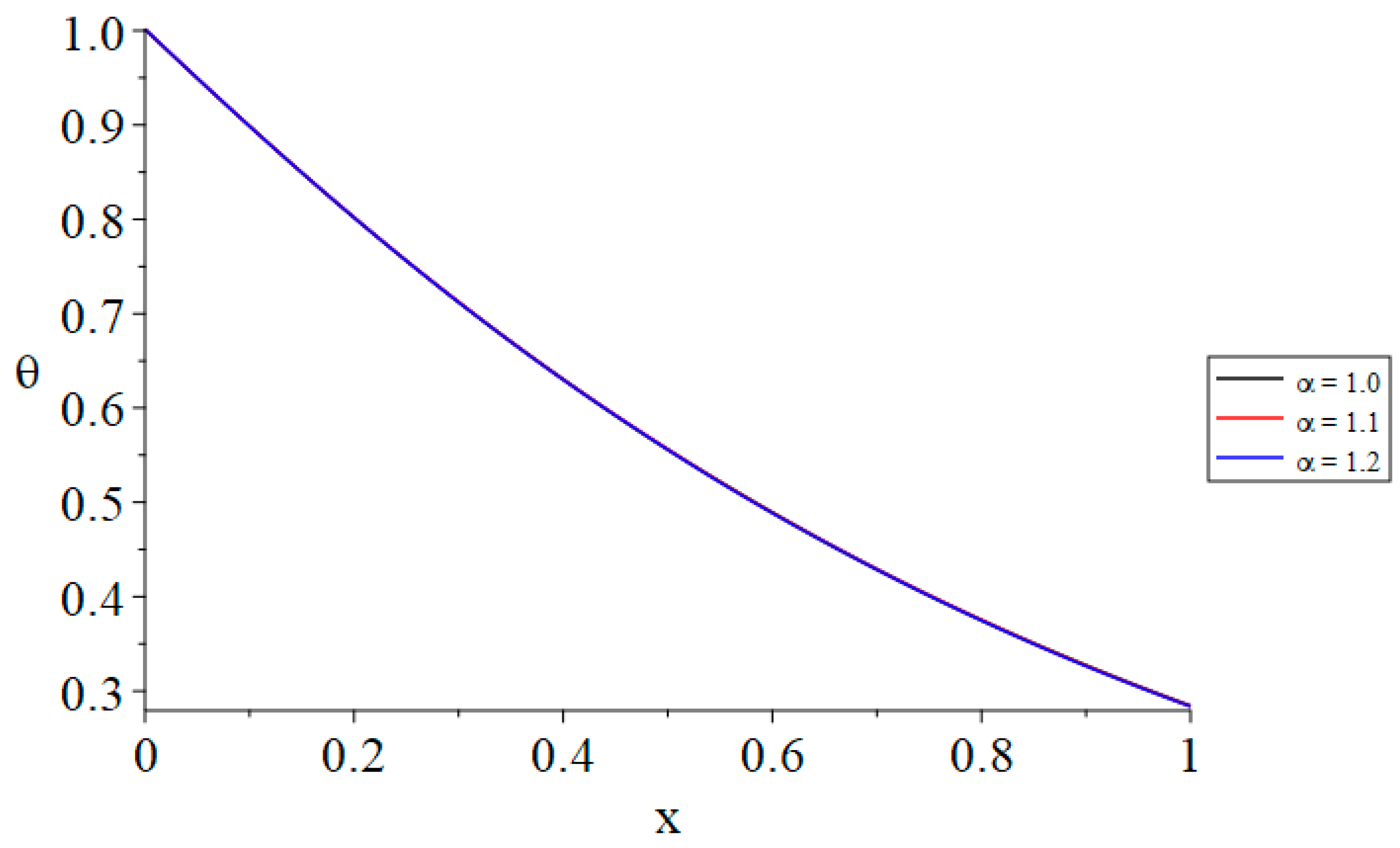
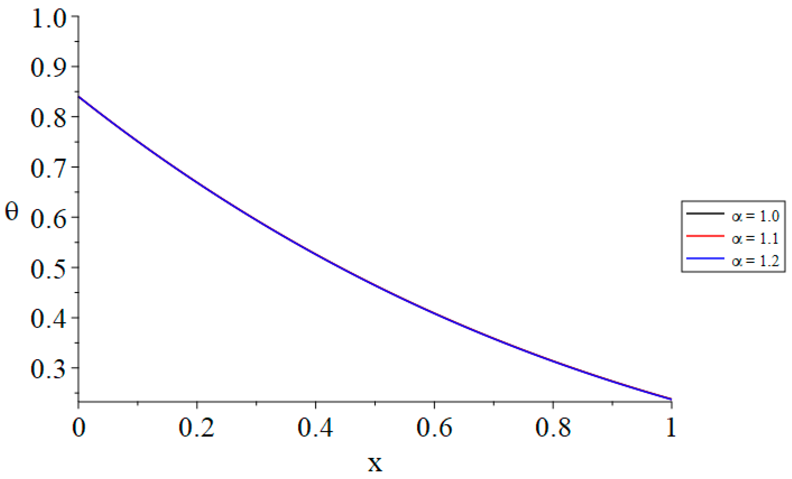
• The time-fractional parameter of Maxwell’s equations does not influence the temperature distribution.
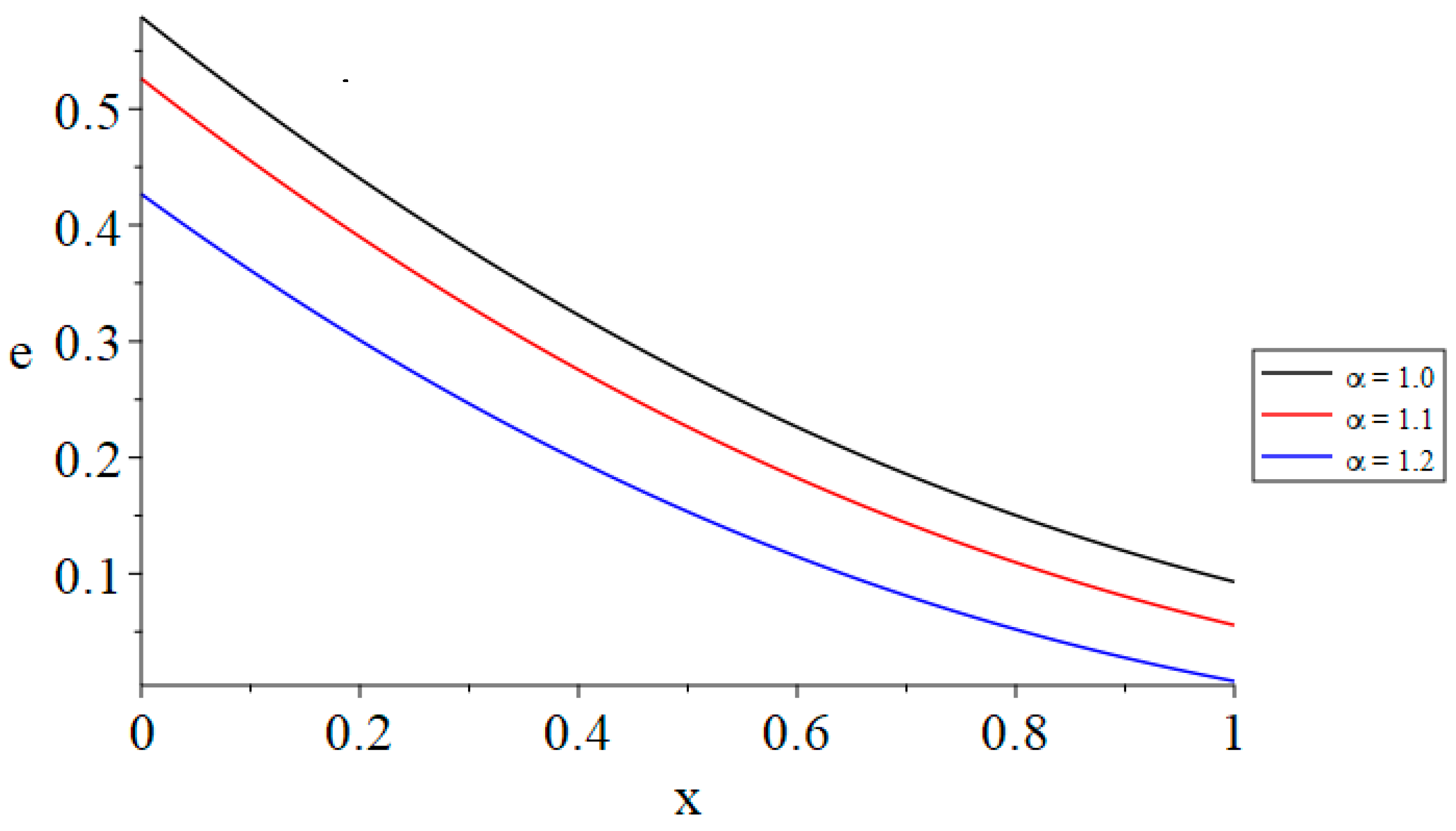
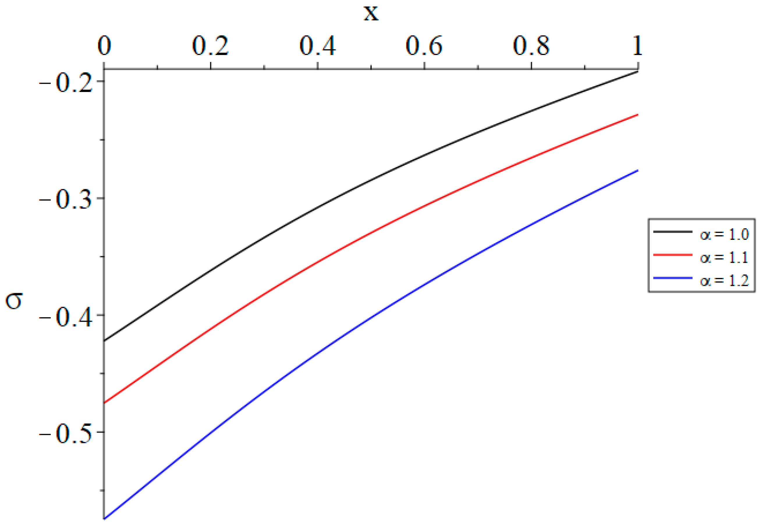
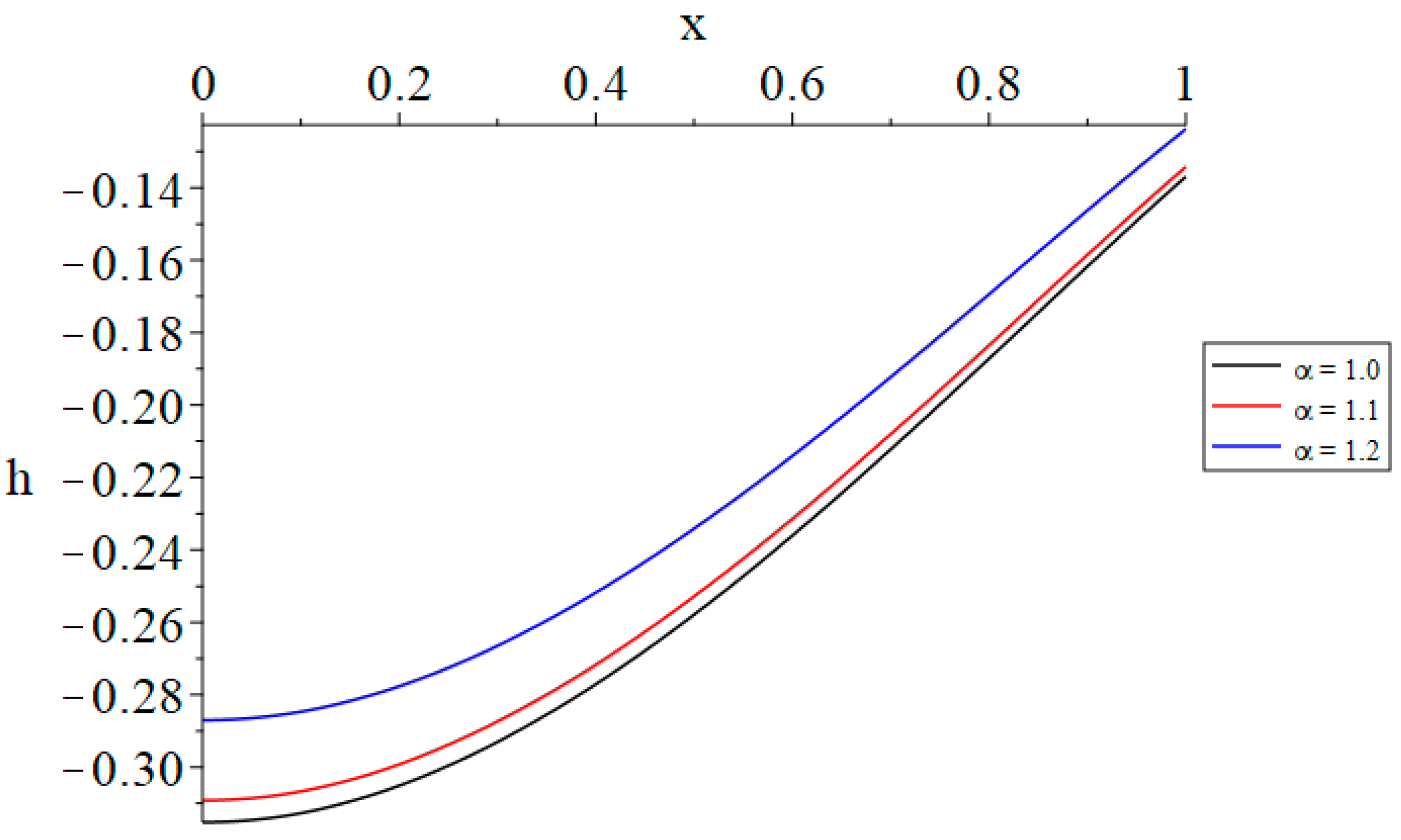
• The time-fractional parameter of Maxwell’s equations substantially influences the strain, displacement, stress, and induced magnetic and electric fields.
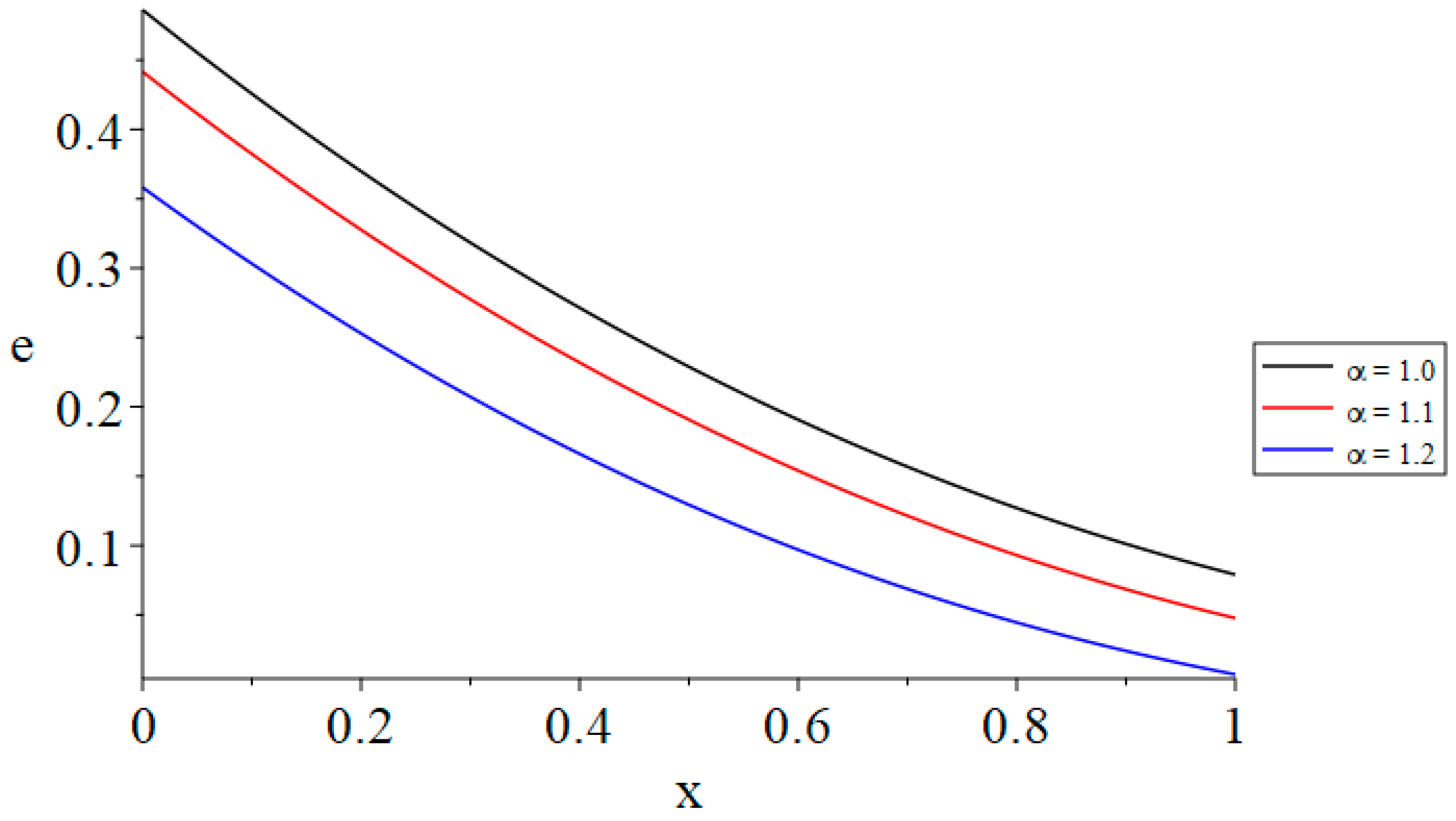
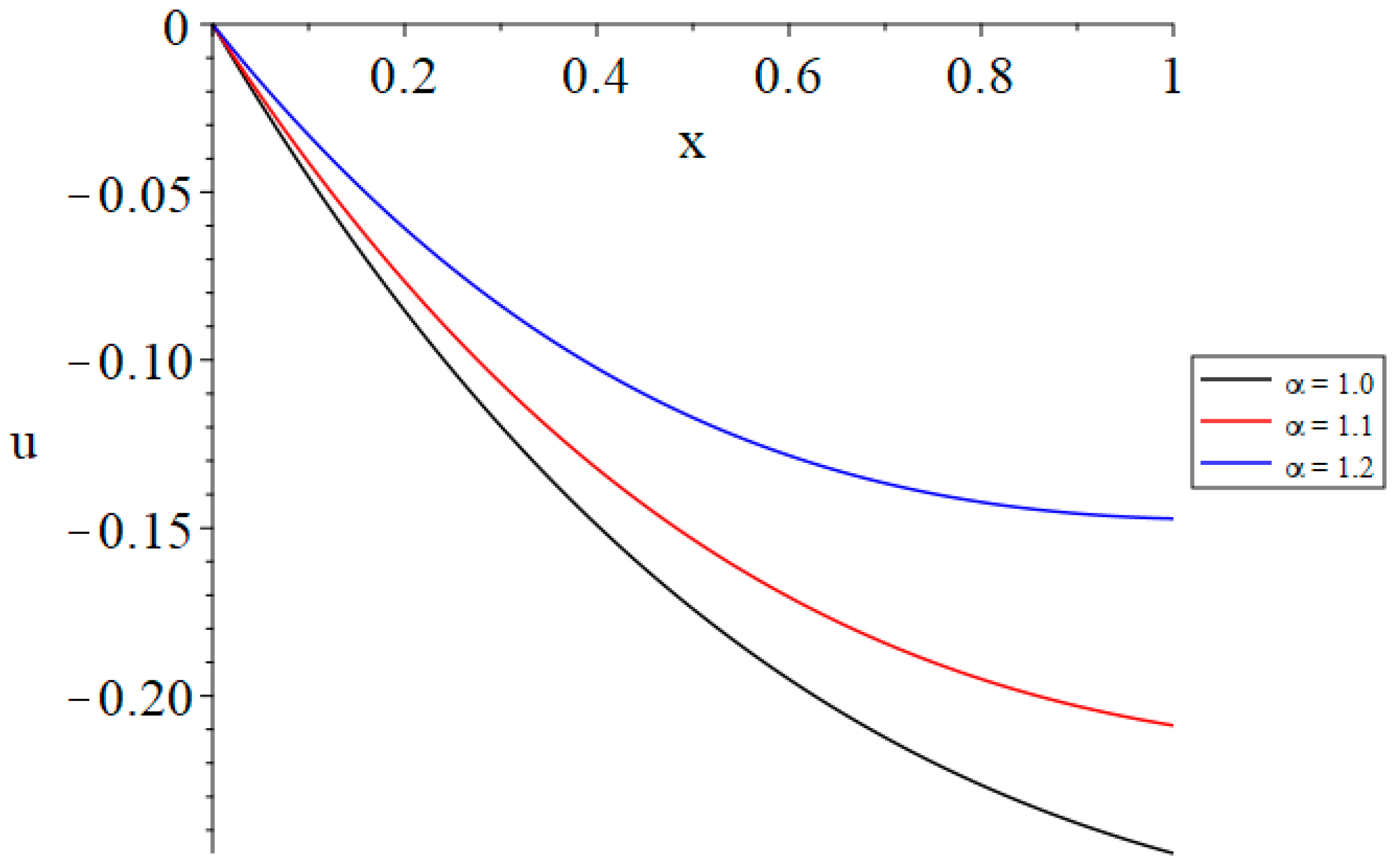
• Increasing the value of the time-fractional parameter of Maxwell’s equations results in a reduction in the volumetric dilatation, the absolute magnitude of the displacement, and the generated magnetic field.
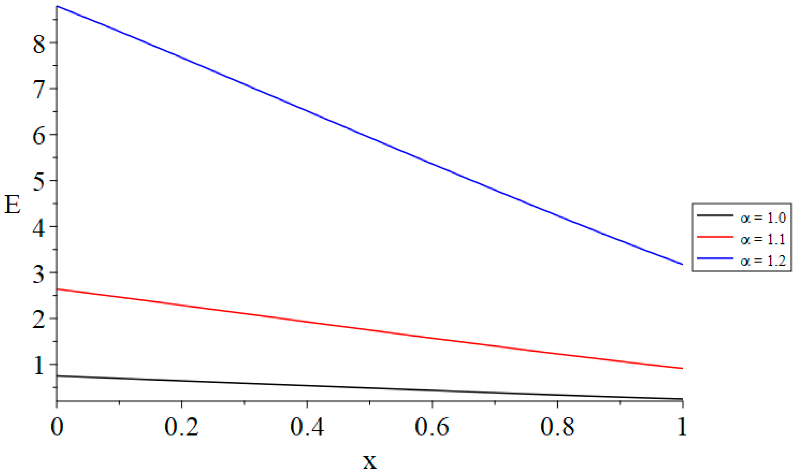
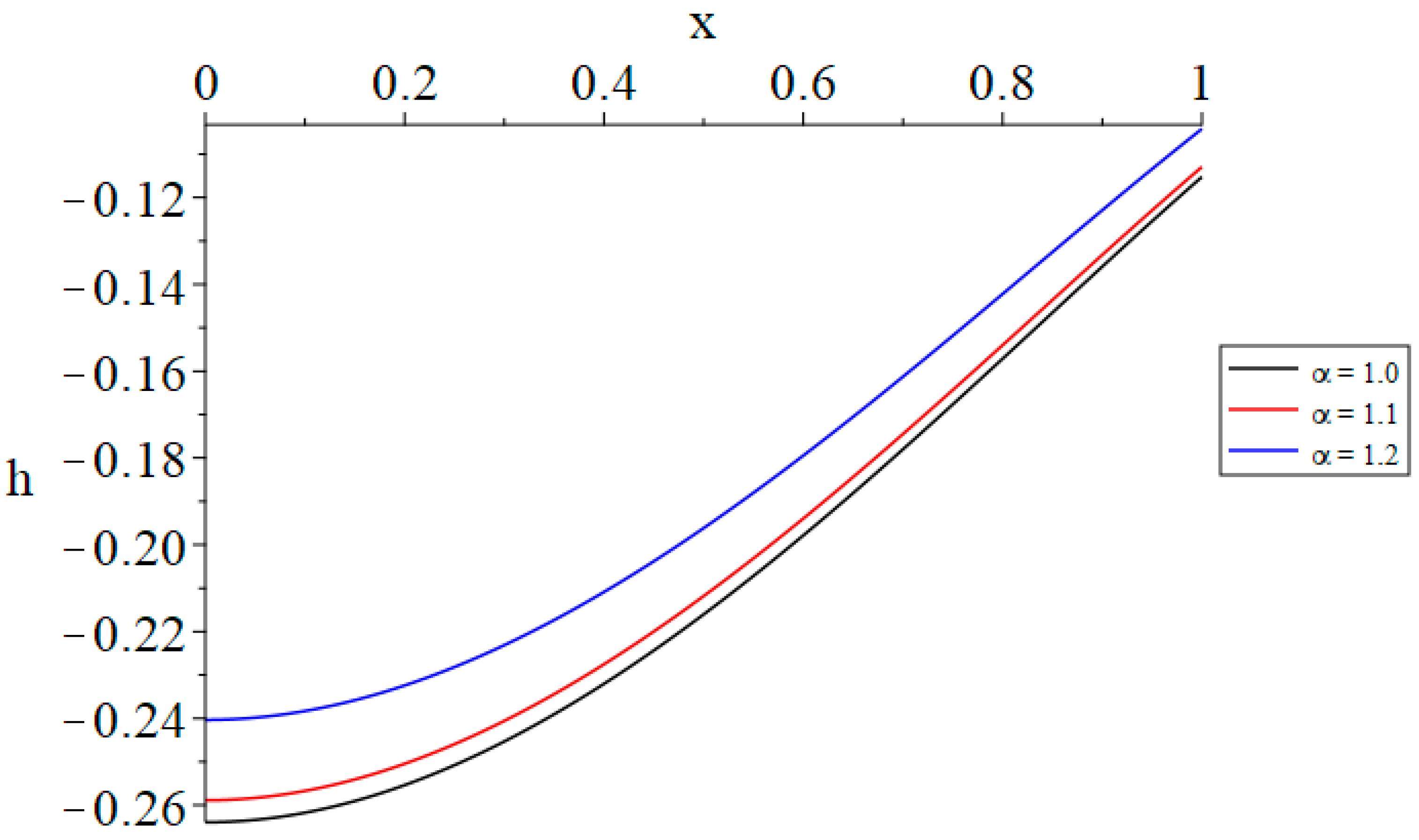
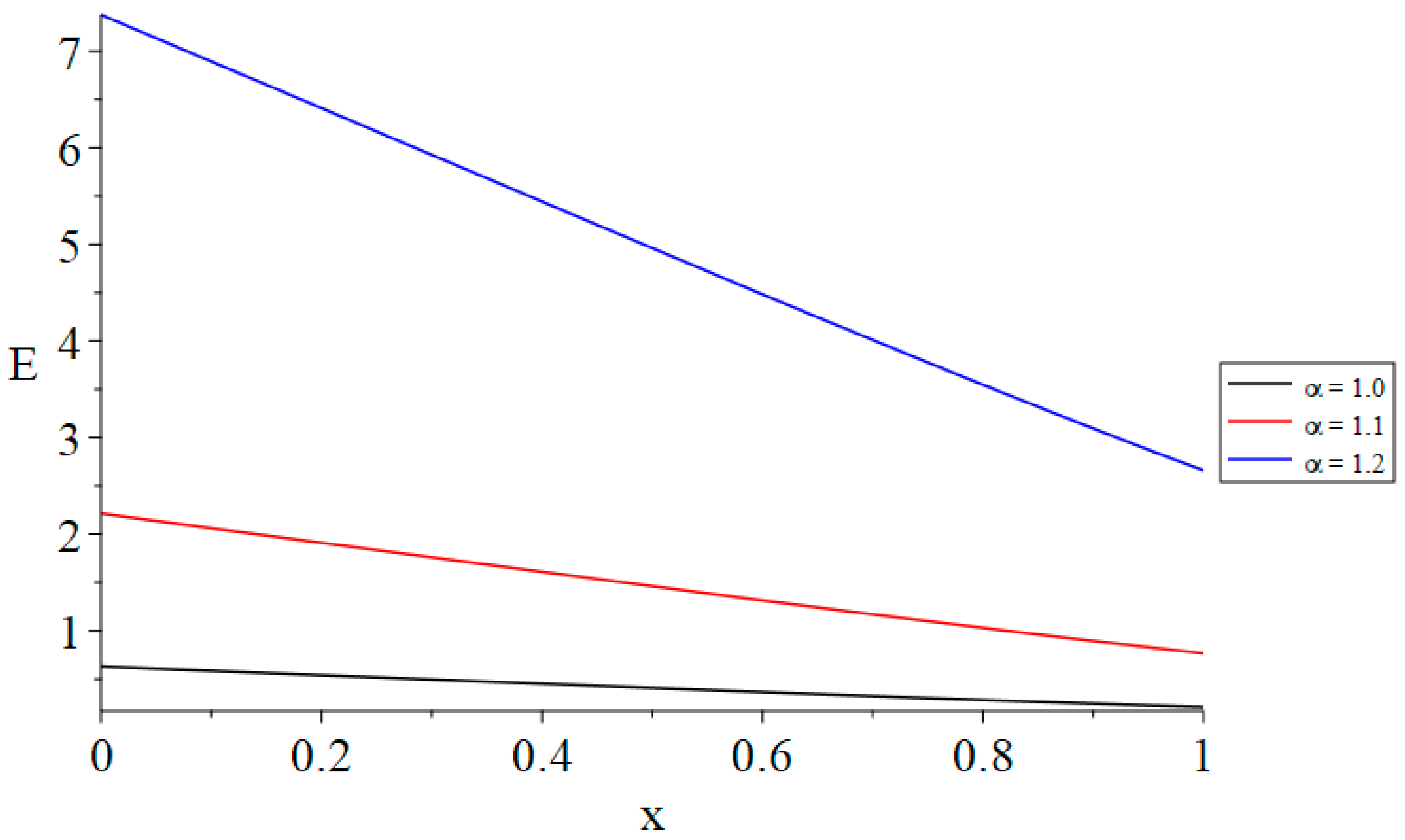
• Increasing the value of the time-fractional parameter of Maxwell’s equations results in heightened stress and an augmented induced electric field.
• The time-fractional parameter of Maxwell’s equations acts as a barrier to deformation, displacement, and the induced magnetic field, while simultaneously catalyzing the created stress and electric field through the material.
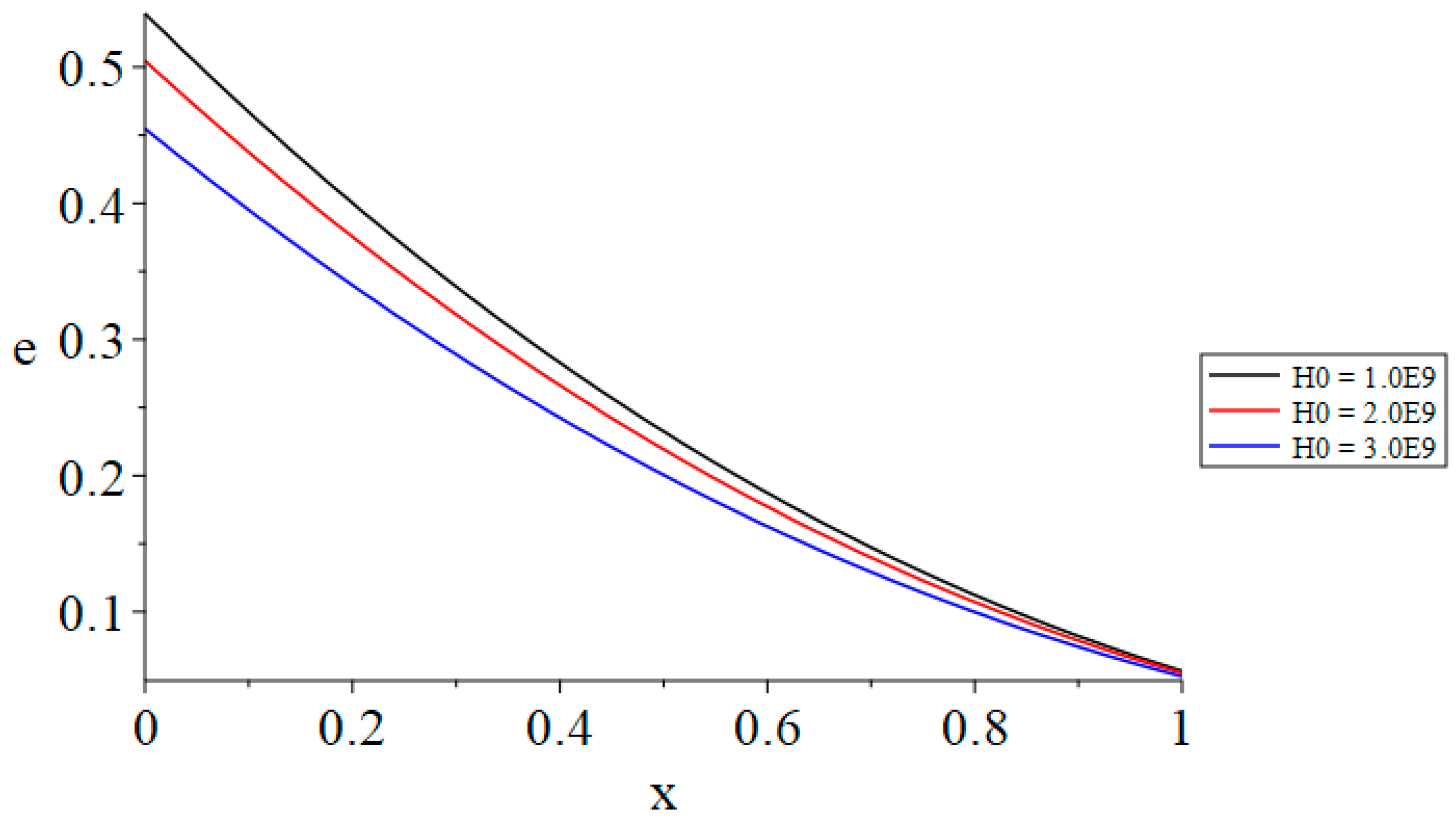
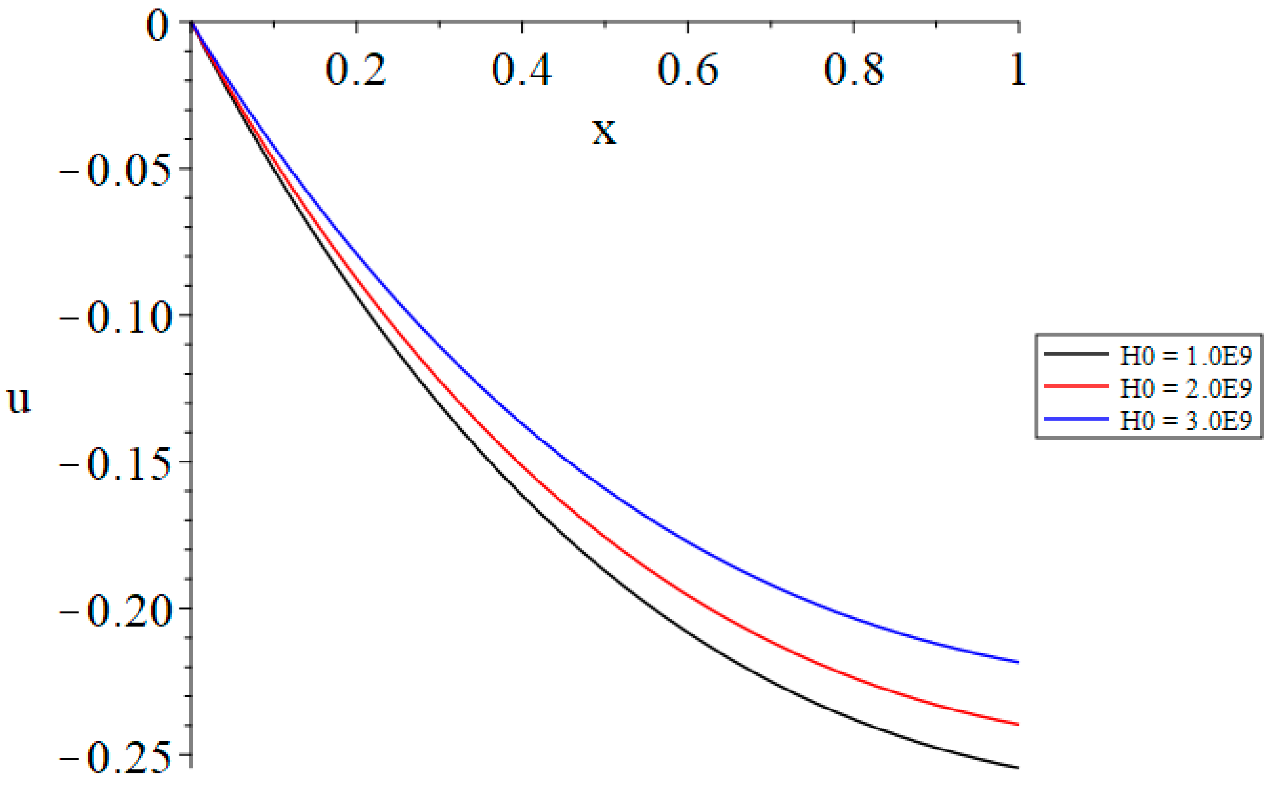
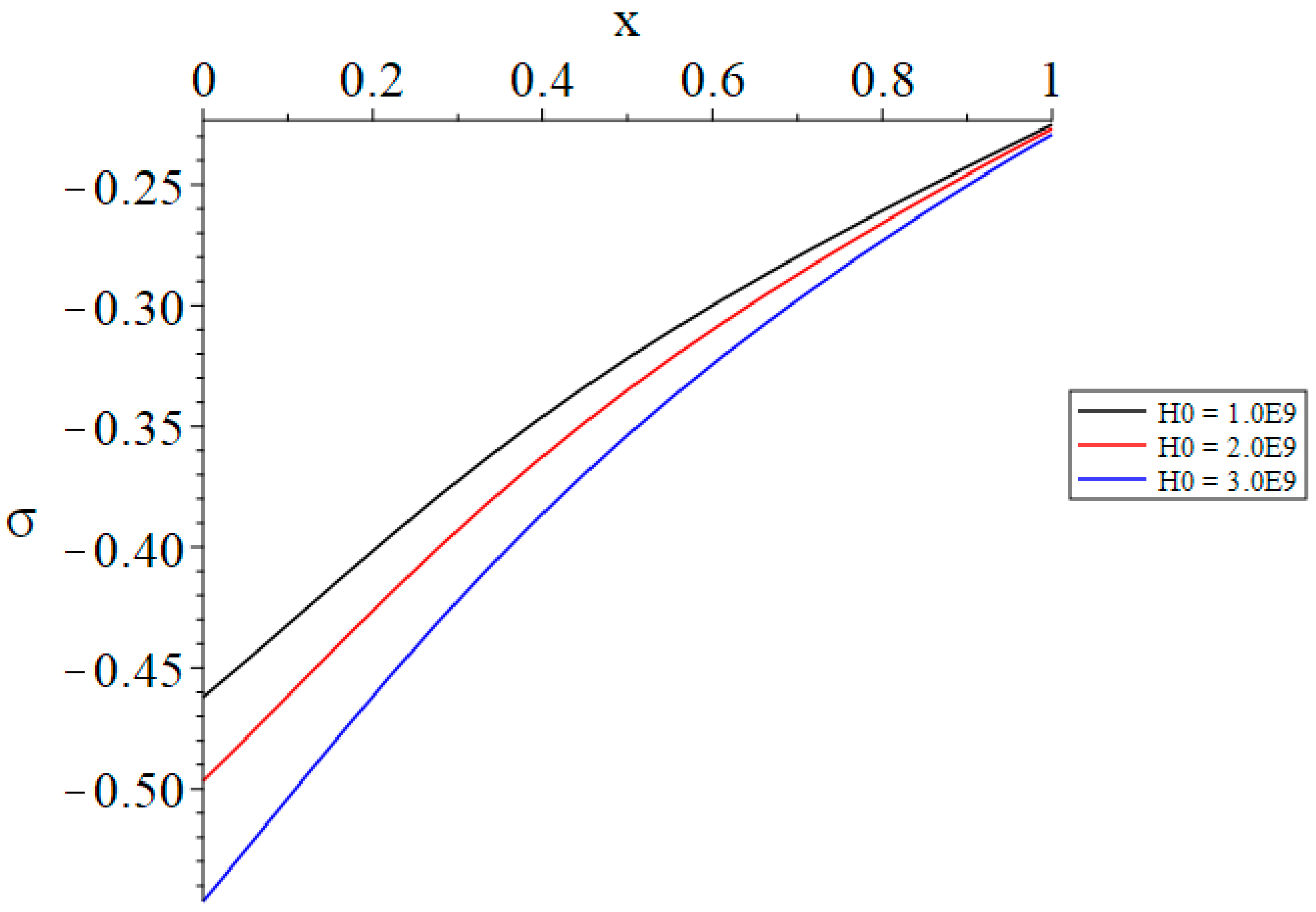
• The magnitude of the primary magnetic field substantially influences the distribution of the volumetric dilatation, displacement, stress, induced magnetic field, and induced electric field, but does not impact the temperature increase.
• The time-fractional parameter of Maxwell’s equations, ramp-time heat parameter, and primary magnetic field can be utilized to modulate the propagation of mechanical waves in magnetothermoelastic materials.
• The ramp-time heat parameter plays a vital role in the behavior of the thermal, mechanical, and electromagnetic waves.

References

1. Hetnarski, R.B.; Eslami, M.R.; Hetnarski, R.B.; Eslami, M.R. Basic laws of thermoelasticity. In Thermal Stresses—Advanced Theory and Applications; Springer: Cham, Switzerland, 2019; pp. 1–43. [Google Scholar]
2. Biot, M.A. Thermoelasticity and irreversible thermodynamics. J. Appl. Phys. 1956, 27, 240–253. [Google Scholar] [CrossRef]
3. Lord, H.W.; Shulman, Y. A generalized dynamical theory of thermoelasticity. J. Mech. Phys. Solids 1967, 15, 299–309. [Google Scholar] [CrossRef]
4. Sherief, H.H.; Darwish, A.A. A short time solution for a problem in thermoelasticity of an infinite medium with a spherical cavity. J. Therm. Stress. 1998, 21, 811–828. [Google Scholar] [CrossRef]
5. Othman, M.I. Relaxation effects on thermal shock problems in an elastic half-space of generalized magneto-thermoelastic waves. Mech. Mech. Eng. 2004, 7, 165–178. [Google Scholar]
6. Sherief, H.H.; Yosef, H.M. Short time solution for a problem in magnetothermoelasticity with thermal relaxation. J. Therm. Stress. 2004, 27, 537–559. [Google Scholar] [CrossRef]
7. Ezzat, M.A.; Youssef, H.M. Generalized magneto-thermoelasticity in a perfectly conducting medium. Int. J. Solids Struct. 2005, 42, 6319–6334. [Google Scholar] [CrossRef]
8. Othman, M.I. Generalized Electromagneto-Thermoelastic Plane Waves by Thermal Shock Problem in a Finite Conductivity Half-Space with One Relaxation Time. Multidiscip. Model. Mater. Struct. 2005, 1, 231–250. [Google Scholar] [CrossRef]
9. Abbas, I.A. Generalized magneto-thermoelasticity in a nonhomogeneous isotropic hollow cylinder using the finite element method. Arch. Appl. Mech. 2009, 79, 41–50. [Google Scholar] [CrossRef]
10. Othman, M.I.; Lotfy, K. Two-dimensional problem of generalized magneto-thermoelasticity with temperature dependent elastic moduli for different theories. Multidiscip. Model. Mater. Struct. 2009, 5, 235–242. [Google Scholar] [CrossRef]
11. Ezzat, M.A.; Youssef, H.M. Generalized magneto-thermoelasticity for an infinite perfect conducting body with a cylindrical cavity. Mater. Phys. Mech. 2013, 18, 156–170. [Google Scholar]
12. Sarkar, N. Generalized magneto-thermoelasticity with modified Ohm’s Law under three theories. Comput. Math. Model. 2014, 25, 544–564. [Google Scholar] [CrossRef]
13. Ezzat, M.A.; El-Karamany, A.S.; El-Bary, A.A. Electro-magnetic waves in generalized thermo-viscoelasticity for different theories. Int. J. Appl. Electromagn. Mech. 2015, 47, 95–111. [Google Scholar] [CrossRef]
14. Othman, M.I.; Song, Y. Effect of the thermal relaxation and magnetic field on generalized micropolar thermoelasticity. J. Appl. Mech. Tech. Phys. 2016, 57, 108–116. [Google Scholar] [CrossRef]
15. Lotfy, K.; Gabr, M. Electromagnetic field of Surface waves propagation in fiber-reinforced generalized thermoelastic medium. J. Niger. Math. Soc. 2017, 36, 239–286. [Google Scholar] [CrossRef]
16. Sadeghi, M.; Kiani, Y. Generalized magneto-thermoelasticity of a layer based on the Lord–Shulman and Green–Lindsay theories. J. Therm. Stress. 2022, 45, 319–340. [Google Scholar] [CrossRef]
17. Khader, S.; Marrouf, A.; Khedr, M. Influence of Electromagnetic Generalized Thermoelasticity Interactions with Nonlocal Effects under Temperature-Dependent Properties in a Solid Cylinder. Mech. Adv. Compos. Struct. 2023, 10, 157–166. [Google Scholar]
18. Tiwari, R. Magneto-thermoelastic interactions in generalized thermoelastic half-space for varying thermal and electrical conductivity. Waves Random Complex Media 2024, 34, 1795–1811. [Google Scholar] [CrossRef]
19. Daftardar-Gejji, V. Fractional Calculus; Alpha Science International Limited: Oxford, UK, 2013. [Google Scholar]
20. Li, C.; Cai, M. Theory and Numerical Approximations of Fractional Integrals and Derivatives; SIAM: Philadelphia, PA, USA, 2019. [Google Scholar]
21. Green, A.E.; Lindsay, K. Thermoelasticity. J. Elast. 1972, 2, 1–7. [Google Scholar] [CrossRef]
22. Sherief, H.H. Fundamental solution for thermoelasticity with two relaxation times. Int. J. Eng. Sci. 1992, 30, 861–870. [Google Scholar] [CrossRef]
23. Sherief, H.H.; Helmy, K.A. A two-dimensional generalized thermoelasticity problem for a half-space. J. Therm. Stress. 1999, 22, 897–910. [Google Scholar]
24. Ailawalia, P.; Priyanka. Effect of thermal conductivity in a semiconducting medium under modified Green-Lindsay theory. Int. J. Comput. Sci. Math. 2024, 19, 167–179. [Google Scholar] [CrossRef]
25. Guo, Y.; Shi, P.; Ma, J.; Liu, F. Dynamic response of thermoelasticity based on Green-Lindsay theory and Caputo-Fabrizio fractional-order derivative. Int. Commun. Heat Mass Transf. 2024, 159, 108334. [Google Scholar] [CrossRef]
26. Karimipour Dehkordi, M.; Kiani, Y. Lord–Shulman and Green–Lindsay-based magneto-thermoelasticity of hollow cylinder. Acta Mech. 2024, 235, 51–72. [Google Scholar] [CrossRef]
27. Kumar, P.; Prasad, R. An investigation of the thermomechanical effects of mode-I crack under modified Green–Lindsay theory. Arch. Appl. Mech. 2024, 94, 3157–3174. [Google Scholar] [CrossRef]
28. Othman, M.I.; Said, S.M.; Gamal, E.M. A new model of rotating nonlocal fiber-reinforced visco-thermoelastic solid using a modified Green–Lindsay theory. Acta Mech. 2024, 235, 3167–3180. [Google Scholar] [CrossRef]
29. Sharifi, H. Magneto–thermoelastic behavior of an orthotropic hollow cylinder based on Lord–Shulman and Green–Lindsay theories. Acta Mech. 2024, 235, 4863–4886. [Google Scholar] [CrossRef]
30. Al-Lehaibi, E.A.; Youssef, H.M. The influence of the Caputo fractional derivative on time-fractional Maxwell’s equations of an electromagnetic infinite body with a cylindrical cavity under four different thermoelastic theorems. Mathematics 2024, 12, 3358. [Google Scholar] [CrossRef]
31. Al-Lehaibi, E.A.; Youssef, H.M. State-Space Approach to the Time-Fractional Maxwell’s Equations under Caputo Fractional Derivative of an Electromagnetic Half-Space under Four Different Thermoelastic Theorems. Fractal Fract. 2024, 8, 566. [Google Scholar] [CrossRef]
32. Almeida, R.; Tavares, D.; Torres, D.F. The Variable-Order Fractional Calculus of Variations; Springer: Berlin/Heidelberg, Germany, 2019. [Google Scholar]
33. Petrás, I. Fractional Derivatives, Fractional Integrals, and Fractional Differential Equations in Matlab; IntechOpen: London, UK, 2011. [Google Scholar]
34. Hilfer, R. Applications of Fractional Calculus in Physics; World Scientific: Singapore, 2000. [Google Scholar]
35. Baleanu, D.; Golmankhaneh, A.K.; Golmankhaneh, A.K.; Baleanu, M.C. Fractional electromagnetic equations using fractional forms. Int. J. Theor. Phys. 2009, 48, 3114–3123. [Google Scholar] [CrossRef]
36. Lazo, M.J. Gauge invariant fractional electromagnetic fields. Phys. Lett. A 2011, 375, 3541–3546. [Google Scholar] [CrossRef]
37. Jaradat, E.; Hijjawi, R.; Khalifeh, J. Maxwell’s equations and electromagnetic Lagrangian density in fractional form. J. Math. Phys. 2012, 53, 033505. [Google Scholar] [CrossRef]
38. Ortigueira, M.D.; Rivero, M.; Trujillo, J.J. From a generalised Helmholtz decomposition theorem to fractional Maxwell equations. Commun. Nonlinear Sci. Numer. Simul. 2015, 22, 1036–1049. [Google Scholar] [CrossRef]
39. Stefański, T.P.; Gulgowski, J. Formulation of time-fractional electrodynamics based on Riemann-Silberstein vector. Entropy 2021, 23, 987. [Google Scholar] [CrossRef] [PubMed]
40. Wang, B.; Kestelyn, X.; Kharazian, E.; Grolet, A. Application of Normal Form Theory to Power Systems: A Proof of Concept of a Novel Structure-Preserving Approach. In Proceedings of the 2024 IEEE Power & Energy Society General Meeting (PESGM), Seattle, WA, USA, 21–25 July 2024; pp. 1–5. [Google Scholar]
41. Avazzadeh, Z.; Hassani, H.; Agarwal, P.; Mehrabi, S.; Javad Ebadi, M.; Hosseini Asl, M.K. Optimal study on fractional fascioliasis disease model based on generalized Fibonacci polynomials. Math. Methods Appl. Sci. 2023, 46, 9332–9350. [Google Scholar] [CrossRef]
42. Alam, M.; Haq, S.; Ali, I.; Ebadi, M.; Salahshour, S. Radial basis functions approximation method for time-fractional fitzhugh–nagumo equation. Fractal Fract. 2023, 7, 882. [Google Scholar] [CrossRef]
43. Machado, J.T.; Jesus, I.S.; Galhano, A.; Cunha, J.B. Fractional order electromagnetics. Signal Process. 2006, 86, 2637–2644. [Google Scholar] [CrossRef]
44. Youssef, H.M. Theory of fractional order generalized thermoelasticity. J. Heat Transfer. 2010, 132, 061301. [Google Scholar] [CrossRef]
45. Youssef, H.M. Theory of generalized thermoelasticity with fractional order strain. J. Vib. Control 2016, 22, 3840–3857. [Google Scholar] [CrossRef]
46. Tzou, D.; Guo, Z.-Y. Nonlocal behavior in thermal lagging. Int. J. Therm. Sci. 2010, 49, 1133–1137. [Google Scholar] [CrossRef]
47. Özisik, M.; Tzou, D. On the Wave Theory in Heat Conduction; ASME-Publications: New York, NY, USA, 1994. [Google Scholar]
Figure 1. The isotropic, homogeneous, generalized, thermoelastic, and electromagnetic half-space exposed to Caputo fractional-order Maxwell’s equations.
Mathematics 13 01468 g001
Figure 2. Distribution of temperature increment for t = t0 = 1.0, H0 = 1.0 × 10⁹.
Mathematics 13 01468 g002
Figure 3. Distribution of volumetric deformation for t = t0 = 1.0, H0 = 1.0 × 10⁹.
Mathematics 13 01468 g003
Figure 4. Distribution of displacement for t = t0 = 1.0, H0 = 1.0 × 10⁹.
Mathematics 13 01468 g004
Figure 5. Distribution of stress for t = t0 = 1.0, H0 = 1.0 × 10⁹.
Mathematics 13 01468 g005
Figure 6. The distribution of the induced magnetic field for t = t0 = 1.0, H0 = 1.0 × 10⁹.
Mathematics 13 01468 g006
Figure 7. The distribution of the induced electric field for t = t0 = 1.0, H0 = 1.0 × 10⁹.
Mathematics 13 01468 g007
Figure 8. Distribution of temperature increment for t < t0, H0 = 1.0 × 10⁹.
Mathematics 13 01468 g008
Figure 9. Distribution of volumetric deformation for t < t0, H0 = 1.0 × 10⁹.
Mathematics 13 01468 g009
Figure 10. Distribution of displacement for t < t0, H0 = 1.0 × 10⁹.
Mathematics 13 01468 g010
Figure 11. Distribution of stress for t < t0, H0 = 1.0 × 10⁹.
Mathematics 13 01468 g011
Figure 12. The distribution of the induced magnetic field for t < t0, H0 = 1.0 × 10⁹.
Mathematics 13 01468 g012
Figure 13. The distribution of the induced electric field for t < t0, H0 = 1.0 × 10⁹.
Mathematics 13 01468 g013
Figure 14. Distribution of temperature increment for t = t0, α = 1.1.
Mathematics 13 01468 g014
Figure 15. Distribution of volumetric dilatation for t = t0, α = 1.1.
Mathematics 13 01468 g015
Figure 16. Distribution of displacement for t = t0, α = 1.1.
Mathematics 13 01468 g016
Figure 17. Distribution of stress for t = t0, α = 1.1.
Mathematics 13 01468 g017
Figure 18. The distribution of the induced magnetic field for t = t0, α = 1.1.
Mathematics 13 01468 g018
Figure 19. The distribution of the induced electric field for t = t0, α = 1.1.
Mathematics 13 01468 g019