Financing Newsvendor with Trade Credit and Bank Credit Portfolio

Abstract

Trade credit is a crucial component of supply chain financing, enabling businesses to manage cash flow and optimize inventory levels. This study delves into the application and implications of multiple trade credit types with different repayment periods and financing costs in a supply chain, encompassing short-term trade credit concatenated with bank financing, long-term trade credit, and a trade credit portfolio. Using a two-stage newsvendor model, we analyze the impact of different trade credit types on supply chain profitability under various scenarios. When facing multiple trade credit types, the retailer prefers financing from the trade credit type that has a lower marginal cost, and the resulting form of financing ensures an equal expected cost of each financing type. The analysis shows that in the case of a monopoly supplier, a long-term credit supplier’s profit is higher than that of a short-term credit supplier. Meanwhile, when the bank interest rate is sufficiently high, the retailer’s profit is highest under the trade credit portfolio mode, whereas when the bank interest rate is sufficiently low, the retailer’s profit is highest under the single short-term credit model. Comparing the effects of different financing modes, we find that there is no optimal financing mode for the overall profit of the supply chain.

1. Introduction

Trade credit, which allows a certain time interval between the delivery date and the payment date, is an effective way to alleviate the shortage of funds in a supply chain. Trade credit is important for firms’ inventory investment, as the amount of trade credit owed by buyers is 3.3 times the total size of bank loans in the US [1], and approximately a quarter of the total assets of small and medium-sized companies in the US are in the form of trade credit [2]. Thus, trade credit is one of the major components of supply chain financing, as it allows sellers to discriminate on price and incur smaller transaction costs in case of default [3]. Trade credit can also reduce moral hazard by mitigating information asymmetry [4,5,6] and lower the overall financing costs for the supply chain by pooling liquidity buffers [7]. However, trade credit debt transmits the risk of default across the entire supply chain when trade credit providers have insufficient accounts receivable to pay their accounts payable. Therefore, it is important for sellers who enjoy the convenience of trade credit to manage their defaults. For example, Zara relies on trade credit from fabric suppliers to place seasonal orders months in advance. If a new collection underperforms, unsold inventory strains cash flow, potentially delaying payments to suppliers and triggering chain-wide liquidity risks.

One of the most important attributes of trade credit is the timing of payment. For instance, companies in the food retailing industries pay an average of almost 30 days beyond their contractually agreed terms. The payment period also influences the cost of the default risk for buyers, as the longer the accounting period is, the more likely the buyer is to receive revenue. In business practice, often, each link in the supply chain is composed of multiple members, and buyers may have many suppliers to choose from. For example, by virtue of its bargaining advantage through market share and order quantity, smartphone brands like Apple obtain longer account periods and lower prices from suppliers that compete for their orders, thus boosting their cash flow via trade credit to invest more in new product innovation and forecast. Chod et al. [8] proposes that when there are multiple products, suppliers who provide trade credit internalize only a part of the benefit.

Motivated by the above empirical evidence and theory, this paper studies the multiple trade credit problem and addresses three questions. First, how do buyers and sellers maximize their profits in a scenario with multiple trade credit types? Second, what are the management implications of multiple trade credit types?

To answer these questions, the paper extends the single-period newsvendor model with external financing to a two-stage newsvendor mode [1]. First, we discuss the single-trade-credit mode, in which either shorter-term trade credit (TC1) or longer-term trade credit (TC2) is available. In the single-TC1 mode, if the bank interest rate is sufficiently low (or high), the capital-constrained retailer orders more (or less) than the capital-abundant retailer, which indicates that the bank increases (or reduces) the retailer’s ordering motivation. The single-TC2 mode is similar to Jing’s model [9]. Then, we discuss the case in which the retailer can choose both TC1 and TC2. In this model, regardless of whether the retailer uses a single-trade-credit type or a trade credit portfolio (TCP), the optimal profit is obtained when the marginal cost is equal to the marginal profit of each channel. Additionally, the analysis shows that the single-TC1 mode (or the TCP mode) is the optimal financing mode for the retailer if the bank interest rate is sufficiently low (or high). Meanwhile, the optimal financing mode for the supplier is the single-TC2 mode. For the overall supply chain, the optimal financing mode depends on the parameters.

Prior research overlooks a view of how firms manage multiple trade credit types. For example, Yang and Birge [1] explore the risk-sharing role of trade credit using a single-period selling-to-the-newsvendor model. Kouvelis and Zhao [4] analyze the optimal trade credit contract when the supplier and retailer may be capital constrained. This paper addresses this gap by establishing a two-stage model that contains two trade credit types, and indicates how a retailer and suppliers should adjust their trade credit order quantities, considering the default risk and the financing cost. The findings could inform businesses with insights to optimize their contract terms, potentially leading to increased efficiency and reduced risk. For practitioners, suppliers can optimize trade credit policies to reduce default risks, while retailers may adjust procurement strategies to balance efficiency and financial stability—especially in industries with high demand volatility (e.g., perishable goods).

The rest of the paper is organized as follows. The Section 2 discusses related research. The Section 3 proposes a TCP model of a capital-constrained retailer and a supplier. The Section 4 derives the optimal solution of the TCP model. The Section 5 summarizes the results and presents the paper’s managerial insights. All of the proofs and technical lemmas are presented in the Appendix A.

2. Literature Review

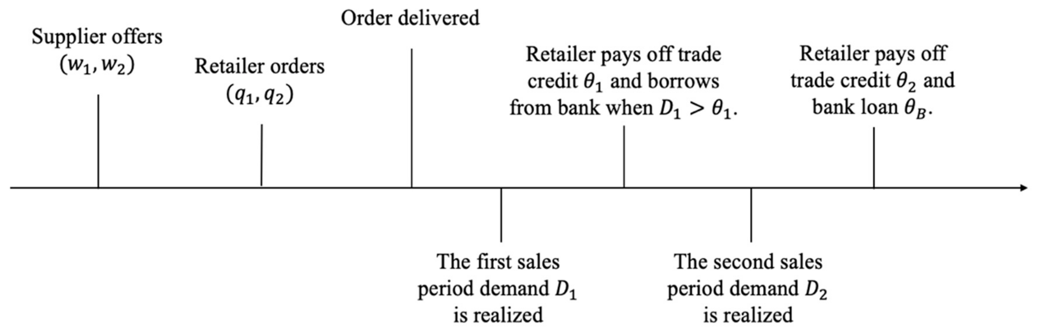
This paper is closely related to the literature on the operation–finance interface, inventory management under trade credit, and bank credit financing.

The research of the operation–finance interface can be traced back at least to Beranek [10], who suggests that inventory decision-making needs to consider financing costs. Several papers show that an inventory strategy’s performance depends on capital conditions and financing costs. Archibald et al. [11] propose that when a firm attempts to survive in the market, the ordered inventory quantity does not monotonously change with the increase in initial cash. Li et al. [12] propose that the basic stock level of the optimal dividend company should be lower than that of the company with the largest profit. Lai et al. [13] propose that suppliers sell part of their inventory to retailers through booking orders to share the default risk if financial constraints exist. Luo [14] suggests that the value of cash pooling can be significant when demand is increasing, and the internal transfer price is low. Financial constraints influence the supply chain parties’ optimal strategy and their performances [15,16,17,18,19,20].

In the operation–finance interface literature, trade credit is one of the most commonly studied approaches adopted by supply chain participants [21]. The trade credit literature goes back at least to Haley and Higgins [22], who study how to manage the order quantity and payment period to maximize the surplus of trade credit. Recent research examines trade credit theoretically and empirically under different frameworks [23,24,25,26,27,28]. Yan and He [29] examine how multiple attributes, including monetary factors (sales profit and bankruptcy cost) and non-monetary factors (service level), influence decision-making in trade credit finance using the multi-attribute utility (MAU) criterion. Chen et al. [30] conduct an empirical investigation into the influence of trade credit on inventory management, highlighting the indispensable role of trade credit in financing inventory and the potential detrimental consequences of restrictions on trade credit for overall supply chain efficiency. Wang et al. [31] investigate trade credit strategies in a two-echelon supply chain involving retailers with heterogeneous credit ratings.

The literature on trade-credit operation has important insights for this paper. Jing et al. [9] show that trade credit is more effective than bank credit in alleviating double marginalization when the production cost is relatively low, whereas bank credit is more effective in other cases. Based on the selling-to-the-newsvendor model with capital constraint, Yang and Birge [1] discuss the interaction between bank credit and trade credit, and how firms decide their corresponding inventory portfolio. They propose that if the retailer’s cash level is low, the supplier offers two-part terms and the retailer finances inventory using both bank loans and trade credit, otherwise the net terms will be provided. Jing et al. [9] and Yang and Birge [1] provide the two basic models used in this paper. It is more common for firms to use short-term and long-term debts than to use cash transactions. Therefore, this paper establishes a two-stage model to illustrate the different liquidity gaps of different repayment periods.

In addition, several works discuss the operation of trade credit. For example, Babich et al. [32] illustrate that bank loan and trade credit are complementary for the retailer. Reindorp et al. [33] illustrate the information asymmetry between the retailer and the supplier. Kouvelis and Zhao [4] point out that trade credit is an indispensable source of financing for retailers and improves the efficiency of the supply chain, and Cachon [34] proposes that trade credit contracts do not necessarily improve the efficiency of the supply chain in presale. Chod [35], taking the perspective of agency theory, points out that a firm benefits from trade credit financing most when the retailer orders multiple differentiated items from a supplier, and shows that the bankruptcy risk and the limited liability effect are significant. Wang et al. [36] investigate the incentive effects of trade credit within a two-tier supply chain featuring a risk-neutral supplier and a risk-averse retailer, where the retailer’s sales cost is treated as private information, and finds that a rational trade credit contract designed by the supplier can effectively encourage the retailer to report the true cost of goods sold, thus increasing the profitability of the supply chain. Yang et al. [37] use mean-variance to explore the differences between wholesale price contracts under trade credit financing and bank financing. Zhu et al. [38] investigate the supplier’s encroachment decision considering trade credit and bank credit financing.

Our paper is also related to the literature on the motivation of providing trade credit to buyers. There are two major situations: a retailer’s purchase channel with supplier monopoly and multiple suppliers jointly supplying the retailer. In the case of monopoly supplier, Schwartz [39] points out that firms with lower financing costs are willing to provide trade credit to those with productive investment opportunities but limited ability to obtain funds. However, a supplier at a disadvantage of financing will also provide trade credit to the retailer. Kouvelis and Zhao [4] compare trade credit with bank credit and show that the optimal trade credit is cheaper than the bank credit, even if the supplier also needs financing. Hu et al. [7] further propose that trade credit pools the liquidity of the supplier and the retailer, thus reducing the financing cost of the overall supply chain. In this paper, we study the effect of different types of trade credit contracts on the supplier, and find that the payment period affects the performance. When there are multiple competitive suppliers, Chod et al. [8] proposed that suppliers who provide trade credit generate free-riding problems and can only internalize part of the benefits. Peura et al. [40], excluding the influence of trade credit on competition, find that trade credit improves the profit of suppliers participating in price competition. However, in this paper, the supplier’s profit is directly determined by the retailer’s profit, and we further consider the price competition between suppliers in a single-product distribution channel.

3. Model

Based on the actual practice of trade credit, we develop a two-stage newsvendor model because multiple trade credits have differences in payment periods. The newsvendor model is chosen due to its ability to capture the decision-making process under demand uncertainty, which is crucial for understanding the interaction between trade credit and inventory management. We allow suppliers to offer two financing types with different prices and payment periods: shorter-term trade credit (TC1) with bank loan and longer-term trade credit (TC2). The payment period of TC1 is one sales period, and that of TC2 is two sales periods. Existing research overlooks the role of mismatched debt of multiple trade credit types and provides limited insight into how supply chain parties can minimize (maximize) the default risk of loans and the financing cost (profit) when faced with multiple trade credit options featuring different repayment dates and costs. Our model addresses these limitations by considering an inventory financing mix-pricing model, which captures the retailer’s optimal inventory financing choice aiming for Pareto-optimality, and the supplier’s optimal pricing strategy.

Based on a financially constrained selling-to-the-newsvendor model [1], we consider a single-product distribution channel consisting of a supplier (S, “she”) and a retailer (R, “he”) with a two-stage sales period with uncertain demand. Manufacturing is controlled by a monopoly supplier, with a retailer without working capital. The product is perishable and produced by the supplier at a constant marginal production cost $c$, with $0\le c\le 1$, and the retailer sells it at a normalized retail price 1. The retailer only needs to consider the prices of the two types of trade credit and the bank interest rate. At the end of the second sales period, the salvage value is zero.

The market demand is stochastic, and the realized demands in the first sales period, $D_1$, and the second sales period, $D_2$, are realized at the payment date of the TC1 and the TC2, respectively. The cumulative distribution function of demands is $F(D_1,D_2)$, which is absolutely continuous with density $f\left(D_1,D_2\right)>0$ on $[0,\infty )$ and has a finite mean. Under the two-dimension condition, $\forall M\in (0,\infty )$, we define the cumulative probability of realized total demand $P\left(M\right)=\mathrm{Pr}(M<D_1+D_2)$ when $D_1+D_2\in (M,\infty )$, whose marginal variation is $P\left(M\right)=-{\displaystyle \frac{\partial P\left(M\right)}{\partial M}}$, the hazard rate $h\left(M\right)={\displaystyle \frac{p\left(M\right)}{P\left(M\right)}}$, and the generalized failure rate $H\left(M\right)=Mh\left(M\right)$. Consistent with the literature, $h\left(M\right)$ is monotonically increasing in $M$. In addition, we assume that $\forall a<M$, $h\left(D_1<a,M\right)>h\left(D_1>a,M\right)$, which means that the probability of stock-out under a smaller realized demand in the first sales period is larger than that under a larger realized demand in the first sales period. Under the bivariate normal distribution, this assumption holds.

Our two-stage model extends the classic newsvendor framework to incorporate a variety of trade credit options, where the retailer’s order quantity decision needs to take into account the cost of excess inventory. This model is designed for supply chain financing contexts, where (1) the monopolistic supplier reflects concentrated upstream power (e.g., Lenovo’s distributor network); (2) zero retailer working capital isolates trade credit effects from internal financing; and (3) perishable goods with zero salvage value capture industries like fresh produce or fashion, where delayed payment risks are acute.

We assume that the supplier is capital-abundant, and the retailer does not hold any cash. At the end of the first sales period, if the retailer cannot afford the TC1 debt, he must rely on bank finance to avoid bankruptcy. In terms of the bank loan, we assume that there is a framework agreement between the retailer and the bank, that is, the bank interest rate $r_B$ is an exogenous parameter. In addition, we assume that the retailer only accepts the price of TC1 if the bank interest is $(1+r_B)w_1$ and the price of TC2 $w_2$ is equal to or less than retail price 1. Both the retailer and the supplier are risk-neutral and have symmetrical information about the retailer’s financial situation and market demand.

We assume that the retailer fully shares the market information with the supplier. The sequence of events is as follows. First, at time 0, the supplier offers her trade credit contract $(w_1, w_2)$. The retailer then decides his inventory portfolio $(q_1, q_2)$ from TC1 and TC2. When the repayment date of TC1 arrives at the end of the first sales period, the retailer uses the revenue of the first sales period to repay the TC1 debt ${\theta }_1=w_1{q}_1$. If the existing revenue $min(q_1+q_2,D_1)$ is insufficient to fully repay ${\theta }_1$, the retailer borrows from the bank at the exogenous interest rate $r_B$ and repays the remaining debt $B={(w_1{q}_1-D_1)}^{+}$. At the end of the second sales period, the retailer repays the bank loan ${\theta }_B=(1+r_B)B$ and the TC2 debt ${\theta }_2=w_2{q}_2$. If the retailer’s revenue is insufficient to repay both claims, he goes bankrupt. Otherwise, the retailer retains the net revenue after both the bank loan and trade credit are fully repaid. The key notations used are summarized in

Table 1. Notations.

$D_i$	the demand realization of the $i^{th}$ sales period; PDF $f\left(D_1,D_2\right)$, CDF $F(D_1,D_2)$
$w_i$	the price of the shorter-term trade credit ($i=1$) or of the longer-term trade credit ($i=2$)
$r_t$	trade credit early discount; $r_t={\displaystyle \frac{w_2-w_1}{w_1}}$
$q_i$	retailer’s order quantity of the shorter-term trade credit ($i=1$) or of the longer-term trade credit ($i=2$)
$q$	retailer’s total order quantity
$q_N$	well-funded retailer’s order quantity
$r_B$	bank interest rate
${\theta }_i$	debt of the shorter-term trade credit ($i=1$) or of the longer-term trade credit ($i=2$)
${\theta }_B$	bank loan
$c$	unit manufacturing cost
${\pi }_R$	the retailer’s profit; ${\pi }_R^i$ is the retailer’s profit under single-TCi mode
${\pi }_S$	the supplier’s profit; ${\pi }_S^i$ is the supplier’s profit under single-TCi mode; ${\pi }_{Si}$ is the supplier $i$’s profit
$M_R$	the retailer’s marginal income
$M_C^i$	the retailer’s marginal cost of the shorter-term trade credit ($i=1$) or of the longer-term trade credit ($i=2$)
$h$	hazard rate
$H$	general failure rate

.

Following common practice [1], we assume that the bank loan is senior to trade credit. The supplier and retailer aim to maximize their expected profits. The sequence of events is illustrated in Figure 1.

4. Financing with Trade Credit Portfolio

In this section, we first analyze the retailer’s inventory portfolio strategy and the supplier’s pricing decision under the two modes with a single-type trade credit (single TC1 and single TC2). Then, we analyze the TCP mode, where both TC1 and TC2 are provided by a single supplier.

4.1. Single-TC1 Problem

This subsection first analyzes the optimal decision-making by the parties under the single-TC1 mode. When the supplier only provides TC1, the retailer makes a one-off payment inventory financing decision. At the end of the first sales period, the retailer repays the TC1 debt ${\theta }_1$ and borrows the remaining debt ${({\theta }_1-D_1)}^{+}$ from bank at interest rate $r_B$ if $D_1<{\theta }_1$. Then, the retailer repays the bank loan ${\theta }_B$ at the end of the second sales period. Unless the retailer fully repays the bank loan, he goes bankrupt. Thus, the retailer’s expected profit under the single-TC1 mode is $E{[\min \left( q-D_1, D_2\right)-{\theta }_B]}^{+}$. When $\min \left( q,D_1\right)>{\theta }_1$, the retailer obtains the remaining profit in the first sales period and all of the profits in the second sales period $\min \left( q,D_1+D_2\right)-{\theta }_1$. For a given $w_1$, the retailer’s problem under the single-TC1 mode is

$${\pi }_R^1=E{[\min \left( q,D_1+D_2\right)-{r_B\left({\theta }_1-D_1\right)}^{+}-{\theta }_1]}^{+}.$$

(1)

We also have

$${\displaystyle \frac{\partial {\theta }_B}{\partial q_1}}={\displaystyle \frac{w\partial {\theta }_B}{\partial B}}=\left(1+r_B\right)w.$$

(2)

Combining Equations (2) and (A1) of the Appendix A, we have

$${\displaystyle \frac{\partial {\pi }_R^1}{\partial q_1}}=P\left(q_1\right)-w_1\left\{\begin{array}{c}{r}_{B}P\left[{\theta }_1>D_1, {\theta }_1+r_B\left({\theta }_1-D_1\right)\right]\\ +P[r_B{\left({\theta }_1-D_1\right)}^{+}+{\theta }_1]\end{array}\right\}.$$

(3)

For each inventory purchased by the retailer, he pays $w_1$ when the revenue of the first sales period is sufficient to pay off ${\theta }_1$; otherwise, he borrows ${\left({\theta }_1-D_1\right)}^{+}$ from the bank and pays extra bank interest $r_B{w}_1$ to avoid TC1 default.

The supplier’s profit is a determined revenue

$${\pi }_S^1={\theta }_1-c{q}_1.$$

(4)

Then we have the following proposition.

Proposition 1.

Supposing $\left(1+r_B\right)w_1\in [c,1]$, under the single-TC1 mode, (1) the optimal order quantity of the capital-constrained retailer, $q_1^{*}$, is uniquely given by $P\left(q_1^{*}\right)=w_1\left\{\begin{array}{c}{r}_{B}P\left[{\theta }_1>D_1, {\theta }_1+r_B\left({\theta }_1-D_1\right)\right]\\ +P[r_B{\left({\theta }_1-D_1\right)}^{+}+{\theta }_1]\end{array}\right\}$, and the optimal order quantity of the capital-abundant retailer, $q_N$, is uniquely given by $P\left(q_N\right)=w_1$; (2) $q_1^{*}$ is decreasing in $w_1$; (3) $q_1^{*}>q_N$ when $r_B<{\displaystyle \frac{1-P[r_B{\left({\theta }_1-D_1\right)}^{+}+{\theta }_1]}{P\left[{\theta }_1>D_1, {\theta }_1+r_B\left({\theta }_1-D_1\right)\right]}}$ and vice versa.

From the perspective of the supplier, because the retailer can borrow from the bank at the end of the first sales period, the retailer and the bank constitute a capital-abundant retailer. When the supplier offers the TC1 price $w_1$, there is a unique optimal order quantity, $q_1^{*}$, that allows the supplier to accurately predict the retailer’s order quantity and optimize the price. The retailer’s marginal profit $P\left(q_N\right)$ is equal to the marginal cost $w_1$.

For comparison, we consider the case in which the retailer has sufficient funds at the beginning. In this case, the retailer does not need to borrow money from the bank. Thus, his optimal profit is ${\pi }_R^N=E\min \left( q,D_1+D_2\right)-{\theta }_1$, and the retailer’s optimal order quantity is $q_N=P^{-1}\left(w_1\right)$.

${\displaystyle \frac{1-P[r_B{\left({\theta }_1-D_1\right)}^{+}+{\theta }_1]}{P\left[{\theta }_1>D_1, {\theta }_1+r_B\left({\theta }_1-D_1\right)\right]}}$ in Proposition 1(3) can be regarded as the default risk of the retailer’s bank loan under the single-TC1 mode. $1-P[r_B{\left({\theta }_1-D_1\right)}^{+}+{\theta }_1]$ is the probability of the retailer defaulting on the bank loan, and $P\left[{\theta }_1>D_1, {\theta }_1+r_B\left({\theta }_1-D_1\right)\right]$ is the probability that the retailer borrows money from the bank and fully repays ${\theta }_B$ at the end of the second sales period. When the bank interest rate $r_B$ is lower than the bank loan default risk, the retailer takes the bank credit as a tool of risk transfer, the bank shares the bankruptcy risk of the retailer, and the retailer obtains a more relaxed capital constraint than in the case of a capital-abundant retailer.

The optimal wholesale price under the single-TC1 mode is given as follows.

Proposition 2.

Under the single-TC1 mode, $w_1^{*}={\displaystyle \frac{1}{1+r_B}}$ or $w_1^{*}=arg\{{\displaystyle \frac{\partial {\pi }_R^1}{\partial w_1}}=0\}$.

Under the single-TC1 mode, the bank shoulders all of the default risk and the supplier gains a determined revenue. When the supplier sets the TC1 price as the manufacturing cost $c$, her profit is zero; as she increases the price, her profits rise, which indicates that the supplier must create profit from providing TC1. Thus, the optimal TC1 price is given by ${\displaystyle \frac{\partial {\pi }_R^1}{\partial w_1}}=0$ or at the upper limit ${\overline{w}}_1={\displaystyle \frac{1}{1+r_B}}$.

4.2. Single-TC2 Problem

Under the single-TC2 mode, the retailer uses the revenue of the two sales periods to repay the TC2 debt at the end of the second sales period. If the retailer’s income $\min \left( q,D_2\right)=D_2$ is insufficient, then the retailer goes bankrupt, as there will be no additional sales income in future and there is no external financing source. The retailer’s problem is

$${\pi }_R^2=E{[\min \left( q,D_1+D_2\right)-{\theta }_2]}^{+},$$

(5)

and we have

$${\displaystyle \frac{\partial {\pi }_R^2}{\partial q_2}}=P\left(q_2\right)-w_{2}P\left({\theta }_2\right).$$

(6)

Similar to the single-TC1 mode, for each inventory, the retailer pays $w_2$.

The supplier’s problem is

$${\pi }_S^2=\min \left(D_1+D_2, {\theta }_2\right)-c{q}_2.$$

(7)

Then we have the following proposition.

Proposition 3.

Under the single-TC2 mode, (1) the optimal order quantity of the retailer, $q_2^{*}$, is uniquely given by $P\left(q_2\right)=w_{2}P\left({\theta }_2\right)$; (2) $q_2^{*}$ is decreasing in $w_2$.

This case is the trade-credit-financing model of Jing et al. (2012) [9] under a two-dimensional distribution. At the end of the second sales period, the retailer repays the TC2 debt with the total revenue of the two sales periods. Similar to the single-TC1 mode, when the supplier offers $w_2$, there is a unique optimal order quantity $q_2^{*}$. With the TC2 price rising, TC2 is more expensive. At the same time, the marginal profit of the retailer remains $P\left(q_2\right)$. Thus, the retailer reduces $q_2^{*}$.

In propositions 1 and 2, the optimal order quantity holds when marginal cost equals to marginal revenue. Under the single-TC1 mode, the retailer’s marginal cost is composed of the bank interest and the unit purchasing cost, whereas under the single-TC2 mode, the marginal cost is fully determined by the TC2 price.

Proposition 4.

Under the single-TC2 mode, the supplier’s optimal TC2 price is $w_2^{*}=1$. Correspondingly, the retailer’s optimal order $q_2^{*}$ is given by $H\left(q_2^{*}\right)=1$.

Under the single-TC2 mode, ${\pi }_S^2$ increases in $w_2^{*}$. As long as the retailer continues to order, the supplier increases the TC2 price to the upper limit ${\overline{w}}_2=1$. At this time, $w_2^{*}$ equals the retail price, and all of the retailer’s revenue belongs to the supplier. This two-stage model is consistent with the trade credit financing model of Jing et al. (2012) [9]. When the retailer defaults, the supplier shoulders not only the manufacturing cost but also all of the retailer’s default risk. In this situation, the retailer’s optimal order $q_2^{*}$ satisfies $H\left(q_2^{*}\right)=1$.

4.3. TCP Problem

We now consider the case in which the supplier provides both TC1 and TC2. The retailer makes his inventory portfolio decision and then needs to repay the supplier when the first and second sales periods end.

If $D_1<{\theta }_1$, the retailer borrows ${\left({\theta }_1-D_1\right)}^{+}$ from the bank at interest rate $r_B$, repays the bank ${\theta }_B=(1+r_B){\left({\theta }_1-D_1\right)}^{+}$ at the end of the second sales period, and then repays the supplier ${\theta }_2$. If $D_1\ge {\theta }_1$, the retailer uses the remaining revenue in the first sales period and the revenue in the second sales period to repay the supplier ${\theta }_2$. Combining the two cases above, the retailer’s problem is

$${\pi }_R=E{[\min \left( q,D_1+D_2\right)-r_B{\left({\theta }_1-D_1\right)}^{+}-{\theta }_1-{\theta }_2]}^{+}.$$

(8)

Different from the single-trade-credit model, in this model, because of the seniority of the bank loan, the supplier shares what remains of the retailer’s revenue after the retailer repays the bank loan; thus, she shares the bank interest when the retailer defaults. In this case, the supplier’s profit is

$${\pi }_S=E\min [{\left(D_2-{\theta }_B\right)}^{+}+{\left(D_1-{\theta }_1\right)}^{+}, {\theta }_2]+{\theta }_1-cq.$$

(9)

Then we have the following proposition.

Proposition 5.

Given $(w_1, w_2)$, under the TCP mode, the optimal order quantities are as follows: (1) for $r_t\in [0, {\displaystyle \frac{r_{B}P\left[{\theta }_1^1>D_1, r_B\left({\theta }_1^1-D_1\right)\right]}{P\left[r_B{\left({\theta }_1^1-D_1\right)}^{+}+{\theta }_1\right]}})$, $(q_1^{*}, q_2^{*})$ is uniquely given by ${\displaystyle \frac{\partial {\pi }_R}{\partial q_1}}=0$ and ${\displaystyle \frac{\partial {\pi }_R}{\partial q_2}}=0$; (2) for $r_t\in [ {\displaystyle \frac{r_{B}P\left[{\theta }_1^1>D_1, r_B\left({\theta }_1^1-D_1\right)\right]}{P\left[r_B{\left({\theta }_1^1-D_1\right)}^{+}+{\theta }_1\right]}}, \infty )$, $q_2^{*}=0$, and $q_1^{*}$ is uniquely given by ${\displaystyle \frac{\partial {\pi }_R}{\partial q_1}}=0$; (3) for $r_t=0$, $q_1^{*}=0$, and $q_2^{*}$ is uniquely given by ${\displaystyle \frac{\partial {\pi }_R}{\partial q_2}}=0$.

Because the retailer’s profit function is jointly quasi-concave, given $(w_1, w_2)$, there is a unique optimal inventory financing combination.

We define the early payment discount

$$r_t={\displaystyle \frac{w_2-w_1}{w_1}}.$$

(10)

Combining Equations (A1) and (A2) of Appendix A, the relationship between $r_t$ and $r_B$ is illustrated by

$$r_t={\displaystyle \frac{r_B·P({\theta }_1>D_1, r_B\left({\theta }_1-D_1\right)+{\theta }_1+{\theta }_2)}{P(r_B{\left({\theta }_1-D_1\right)}^{+}+{\theta }_1+{\theta }_2)}}.$$

(11)

The retailer’s inventory model is determined by the marginal cost of the two trade credit types. When the retailer only uses TC1, if the marginal cost of TC2 is greater than or equal to the marginal cost of TC1, then $q_2^{*}=0$. Otherwise, the retailer uses both trade credit types at the same time, leading to the following upper limit of the early-payment discount

$${\overline{r}}_t={\displaystyle \frac{r_{B}P\left[{\theta }_1^1>D_1, r_B\left({\theta }_1^1-D_1\right)\right]}{P\left[r_B{\left({\theta }_1^1-D_1\right)}^{+}+{\theta }_1\right]}},$$

(12)

where ${\theta }_1^1$ is given by the optimal order quantity under the single-TC1 mode.

When $w_2=w_1$, the marginal cost of TC1 is greater than or equal to the marginal cost of TC2, so the retailer does not order from TC1. If $w_2>w_1$, the marginal cost of TC1 is lower than that of TC2, so the retailer orders from both trade credit types, always choosing the one with the lower initial price. Then we have the following result.

Lemma 1.

Under the TCP mode, (1) given $w_1$, $q_1^{*}$ is increasing in $w_2$, and $q_2^{*}$ is decreasing in $w_2$; (2) given $w_2$, $q_2^{*}$ is increasing in $w_1$, and $q_1^{*}$ is decreasing in $w_1$; and (3) when the retailer uses both TC1 and TC2, $r_t$ is strictly less than $r_B$.

When the retailer place orders from both TC1 and TC2, given $w_1$ (or $w_2$), the financing cost of TC2 (or TC1) becomes more expensive as $w_2$ (or $w_1$) rises, and the financing cost of $q_1^{*}$ (or $q_2^{*}$) decreases. Therefore, $q_2^{*}$ (or $q_1^{*}$) decreases, and $q_1^{*}$ (or $q_2^{*}$) increases.

If $r_t\ge r_B$, then the marginal cost of TC1 is always less than or equal to that of TC2 and the retailer only orders from TC1. This is why when the retailer uses both TC1 and TC2, the early-payment discount is usually lower than the financing cost of insufficient emergency liquidity (as the emergency loan may not be needed).

Let

$$\begin{array}{l}{\mathsf{{\rm Y}}}_1={\left.{\displaystyle \frac{\partial w_1}{\partial q}}\left\{\begin{array}{c}\left({\displaystyle \frac{\partial q_1}{\left(1+r_B\right)\partial w_1}}+q_1\right)\left\{\begin{array}{c}\mathrm{Pr}\left[{\left(D_2-{\theta }_B\right)}^{+}+{\left(D_1-{\theta }_1\right)}^{+}>{\theta }_2\right]\\ -r_B\mathrm{Pr}\left[{\theta }_1>D_1, {\left(D_2-{\theta }_B\right)}^{+}<{\theta }_2\right]\end{array}\right\}\\ +{\displaystyle \frac{1}{1+r_B}}{\displaystyle \frac{\partial q_2}{\partial w_1}}\mathrm{Pr} [{\left(D_2-{\theta }_B\right)}^{+}+{\left(D_1-{\theta }_1\right)}^{+}>{\theta }_2]\end{array}\right\}\right|}_{w_1={\displaystyle \frac{1}{1+r_B}}},\\ {\mathsf{{\rm Y}}}_2={\left.{\displaystyle \frac{\partial w_1}{\partial q}}\left\{\begin{array}{c}{\displaystyle \frac{\partial q_1}{\partial w_1}}{w}_2\left\{\begin{array}{c}\mathrm{Pr}\left[{\left(D_2-{\theta }_B\right)}^{+}+{\left(D_1-{\theta }_1\right)}^{+}>{\theta }_2\right]\\ -r_B\mathrm{Pr}\left[{\theta }_1>D_1, {\left(D_2-{\theta }_B\right)}^{+}<{\theta }_2\right]\end{array}\right\}\\ +w_2{\displaystyle \frac{\partial q_2}{\partial w_1}}\mathrm{Pr} [{\left(D_2-{\theta }_B\right)}^{+}+{\left(D_1-{\theta }_1\right)}^{+}>{\theta }_2]\end{array}\right\}\right|}_{w_1=w_2},\\ {\mathsf{{\rm Y}}}_3={\left.{\displaystyle \frac{\partial w_1}{\partial q}}\left({\displaystyle \frac{\partial q_1}{\partial w_1}}{\displaystyle \frac{w_2}{1+{\overline{r}}_t}}+q_1+w_2{\displaystyle \frac{\partial q_2}{\partial w_1}}\right)\mathrm{P}\mathrm{r} [{\left(D_2-{\theta }_B\right)}^{+}+{\left(D_1-{\theta }_1\right)}^{+}]\right|}_{w_1={\displaystyle \frac{w_2}{1+{\overline{r}}_t}}}.\end{array}$$

Then we have the following result.

Proposition 6.

Under the single-TCP mode, (1) for a given $w_2$, we have

$$w_1^{*}=\left\{\begin{array}{c}\begin{array}{c}{\displaystyle \frac{1}{1+r_B}}, if w_2>{\displaystyle \frac{1}{1+r_B}} and c>{{\rm Y}}_1,\\ w_2, if w_2\le {\displaystyle \frac{1}{1+r_B}} and c\le {{\rm Y}}_2, \end{array}\\ \begin{array}{c}{\displaystyle \frac{w_2}{1+{\overline{r}}_t}}, if c\ge {{\rm Y}}_3, \\ \mathit{arg}\left\{{\displaystyle \frac{\partial {\pi }_S}{\partial w_1}}=0\right\}, otherwise. \end{array}\end{array}\right.$$

(2) For a given $w_1$, we have

$$w_2^{*}=\left\{\begin{array}{c}{w}_1, if c<{\left.\left(w_1+q_2{\displaystyle \frac{\partial w_2}{\partial q}}\right)\mathit{Pr}\left(D_1+D_2>{\theta }_2\right)\right|}_{w_2=w_1}, \\ \left(1+{\overline{r}}_t\right)w_1, if c>{\left.{\displaystyle \frac{\partial w_2}{\partial q}}\left({\displaystyle \frac{\partial q_1}{\partial w_2}}{w}_1+\left(1+{\overline{r}}_t\right)w_1{\displaystyle \frac{\partial q_2}{\partial w_2}}\right)\mathit{Pr}\left({\left(D_2-{\theta }_B\right)}^{+}+{\left(D_1-{\theta }_1\right)}^{+}\right)\right|}_{w_2=\left(1+{\overline{r}}_t\right)w_1}, \\ \mathit{arg}\left\{{\displaystyle \frac{\partial {\pi }_S}{\partial w_2}}=0\right\}, otherwise.\end{array}\right.$$

It can be verified that the supplier’s profit is unimodal under the bivariate normal distribution. The supplier’s profit under different $w_1$ and $r_t$ is shown in Figure 2. Given either $w_1$ (or $w_2$), $w_2^{\mathrm{*}}$ (or $w_1^{\mathrm{*}}$) is dependent on the manufacturing cost $c$. Intuitively, when $c$ is sufficiently large, unpaid orders incur a great loss to the supplier; thus, the supplier prefers for the retailer to use only TC1 and obtain a determined revenue. Meanwhile, when $c$ is sufficiently small, the supplier pursues a higher order quantity by reducing the TC2 price. In addition, the price assumption $\left(1+r_B\right)w_1\le 1$ creates a pricing restriction for the supplier: if ${\displaystyle \frac{w_2}{1+{\overline{r}}_t}}>{\displaystyle \frac{1}{1+r_B}}$, the TC2 price is so high that the retailer only uses TC1, as per Proposition 5. In all other cases, the supplier provides a TCP contract under which the retailer uses both trade credit types.

Now we consider the profits.

Proposition 7.

(1) Given $w_1$, for

$$c<{\left.{\displaystyle \frac{\partial w_2}{\partial q}}\left({\displaystyle \frac{\partial q_1}{\partial w_2}}{w}_1+\left(1+{\overline{r}}_t\right)w_1{\displaystyle \frac{\partial q_2}{\partial w_2}}\right)\mathit{Pr}\left({\left(D_2-{\theta }_B\right)}^{+}+{\left(D_1-{\theta }_1\right)}^{+}\right)\right|}_{w_2=\left(1+{\overline{r}}_t\right)w_1},$$

the supplier can obtain higher profit by providing a TCP than by providing a single-TC1 contract; (2) given $w_2$, for ${\displaystyle \frac{w_2}{1+{\overline{r}}_t}}<{\displaystyle \frac{1}{1+r_B}}$ and $c<{{\rm Y}}_3$, the supplier can obtain a higher profit by providing a TCP than by providing a single-TC2 contract.

According to Proposition 6, the retailer’s optimal inventory decision under the TCP mode is the same as that under the single-TC1 mode when $w_2^{\mathrm{*}}={\overline{w}}_2$. Thus, when $w_2^{\mathrm{*}}<{\overline{w}}_2$, the supplier’s profit under the TCP mode is higher than that under the single-TC1 mode. According to Proposition 6, the manufacturing cost obeys $c<{\left.{\displaystyle \frac{\partial w_2}{\partial q}}\left({\displaystyle \frac{\partial q_1}{\partial w_2}}{w}_1+\left(1+{\overline{r}}_t\right)w_1{\displaystyle \frac{\partial q_2}{\partial w_2}}\right)\mathrm{Pr}\left({\left(D_2-{\theta }_B\right)}^{+}+{\left(D_1-{\theta }_1\right)}^{+}\right)\right|}_{w_2=\left(1+{\overline{r}}_t\right)w_1}$.

When ${\displaystyle \frac{w_2}{1+{\overline{r}}_t}}>{\displaystyle \frac{1}{1+r_B}}$, TC2 is too expensive for the retailer, and he uses the single-TC1 mode. Therefore, we only consider the case of ${\displaystyle \frac{w_2}{1+{\overline{r}}_t}}<{\displaystyle \frac{1}{1+r_B}}$. If $w_1^{\mathrm{*}}={\underset{\_}{w}}_1$, the retailer’s optimal inventory decision is the same as that under the single-TC2 mode, so when $w_1^{\mathrm{*}}>{\underset{\_}{w}}_1$, the supplier’s profit under the TCP mode is higher than that under the single-TC2 mode. According to Proposition 6, the manufacturing cost obeys $c<{\mathsf{{\rm Y}}}_3$.

4.4. Numerical Analysis

In this subsection, we perform a series of numerical experiments to study the effects of (1) the performance of the overall supply chain and its individual parties, as well as (2) the key parameters of the retailer’s financial situation and market demand. We assume that the market demand follows the bivariate normal distribution with ${\mu }_i=100$, ${\sigma }_i=25,$ and $\rho =0.3$. The following financial parameters are used in all instances unless otherwise stated: $r_B=0.1$, $c=0.2$. These uniform settings allow comparative analysis.

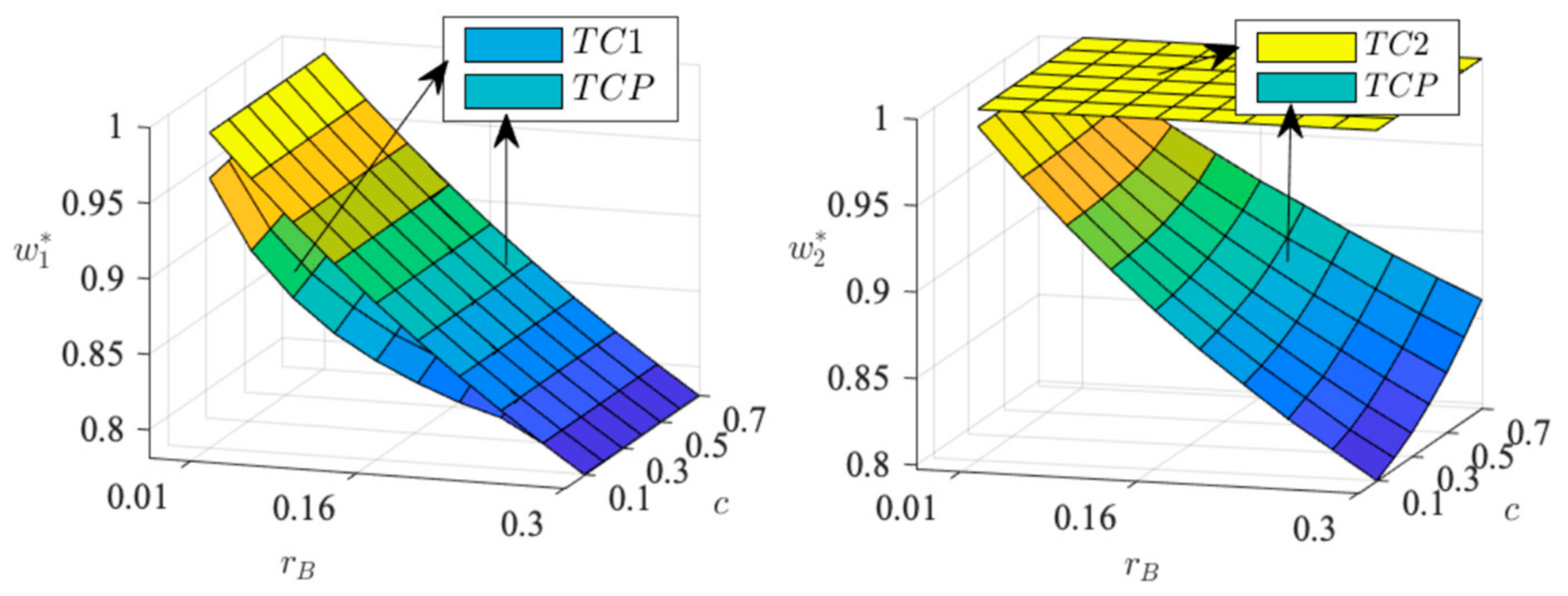
4.4.1. The Supplier’s Price and the Retailer’s Order Quantity

When $c\in \left[0.1, 0.7\right]$ and $r_B\in [0.01, 0.3]$, the optimal price is shown in Figure 3, and the retailer’s optimal order quantity is shown in Figure 4. Because the supplier obtains a determined revenue under the single-TC1 mode, $w_1^{\mathrm{*}}$ under the TCP mode is higher than that under the single-TC1 mode. However, under the single-TC2 mode, the supplier shoulders all of the default risk of the retailer; thus, $w_2^{\mathrm{*}}$ under the single-TC2 mode is the highest among all financing modes. In addition, the order quantity under the single-TC1 mode is the lowest and that under the TCP mode is the highest. An intuitive interpretation is that the retailer can always purchase from a lower-cost trade credit type under the TCP mode, so he orders more inventory than under other financing modes. Under the single-TC1 mode, the retailer aims to reduce the probability of needing a bank loan, which has a higher interest rate than an early-payment discount, so his order quantity under this mode is the lowest.

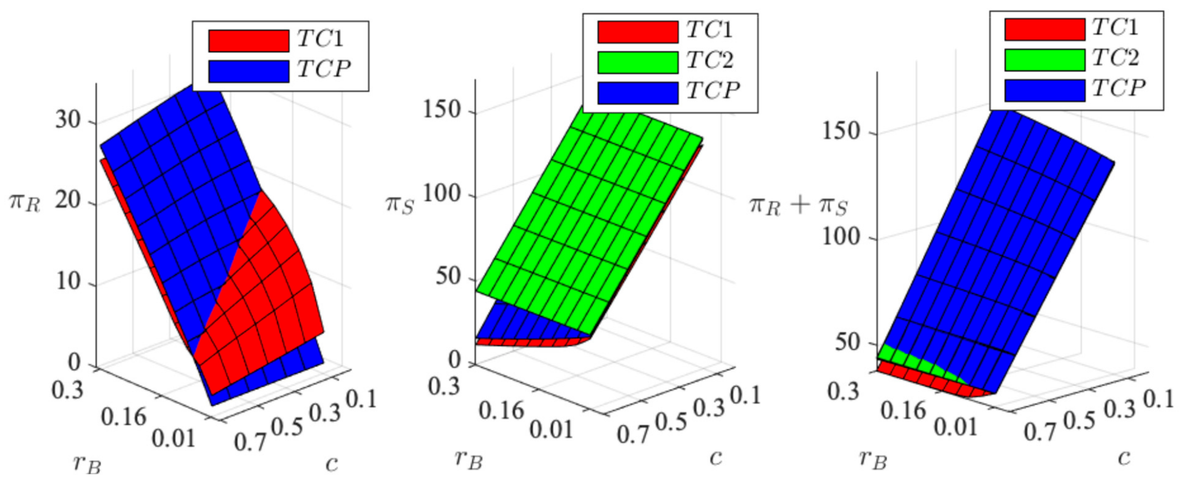
4.4.2. Comparison of the Parties’ Profit

When $c\in \left[0.1, 0.7\right]$ and $r_B\in [0.01, 0.3]$, the parties’ profit under different financing modes is shown in Figure 5.

The retailer’s profit is zero under the single-TC2 mode. Under the single-TC1 mode, when $r_B$ is sufficiently low (or sufficiently high), he has a lower (or higher) total financing cost than that under the TCP mode and can obtain a higher (or lower) profit.

The supplier’s profit under the single-TC2 model is higher than under the other two financing modes because she shoulders all of the default risk from the retailer’s bankruptcy. In addition, her profit under the single-TC1 mode is the lowest, as the optimal price of the single-TC1 mode is lower than that of the single-TC2 mode and the TCP mode.

For the overall supply chain, when the bank interest rate is sufficiently high (or sufficiently low), the total profit under the TCP mode is lower (or higher) than that under the single-TC1 mode. Otherwise, when the manufacturing cost is sufficiently low (or sufficiently high), the total profit under the TCP mode is lower (higher) than that under the single-TC2 mode. As shown in Figure 6, the total profit under the TCP mode in region I is the highest. In addition, the overall supply chain profit is highest under the single TC1 mode in region III, and under the single TC2 mode in region II.

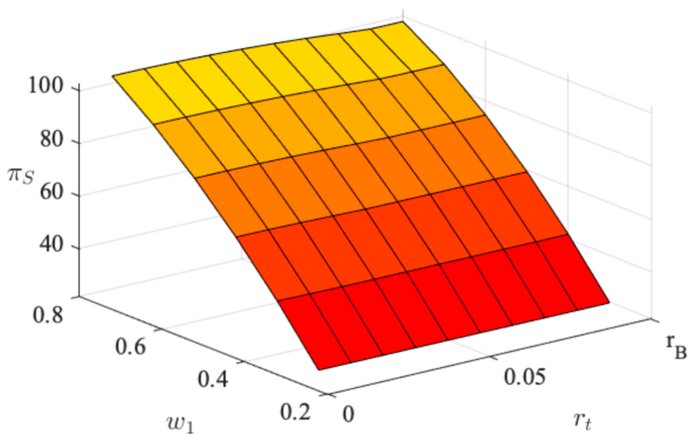
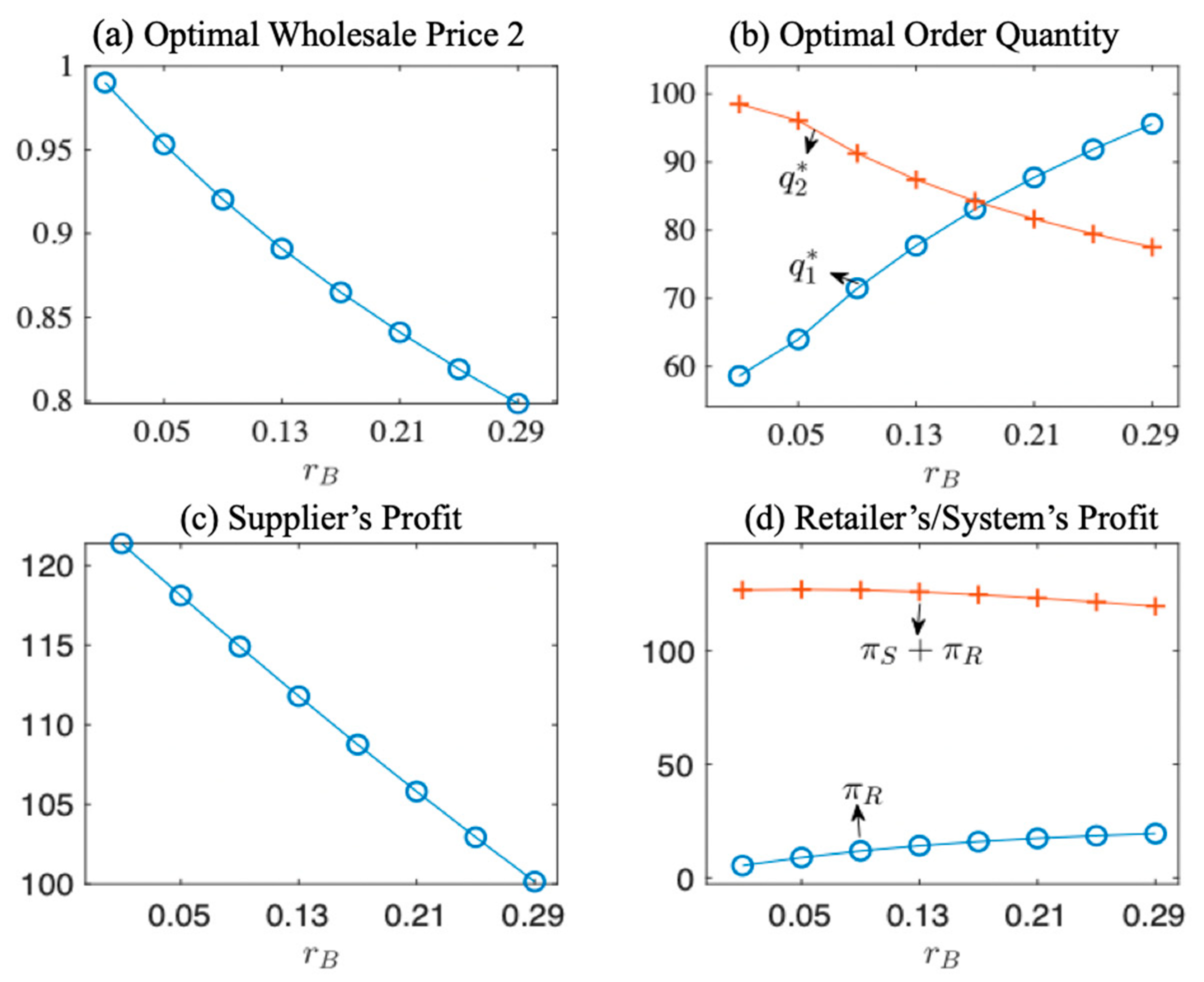
4.4.3. Impact of the Bank Interest Rate

As shown in Figure 7, the optimal order quantity is determined by both the bank interest rate and the price combination, and it ensures that the marginal cost equals the marginal income. In this example, as $r_B$ increases, $w_1^{\mathrm{*}}$ decreases, and the bank interest $r_B{w}_1={\displaystyle \frac{r_B}{1+r_B}}$ increases.

Therefore, when the descending effect of ${\overline{w}}_1$ is greater than the ascending effect of $r_B{w}_1$, the marginal cost of TC1 decreases, and the cost of TC2 increases, it follows that $q_1^{\mathrm{*}}$ increases and $q_2^{\mathrm{*}}$ decreases. For the retailer, the descending effect of price is greater than the ascending effect of bank interest, so the retailer’s profit increases, while the supplier’s profit and the profit of the overall supply chain decrease as the trade credit price decreases.

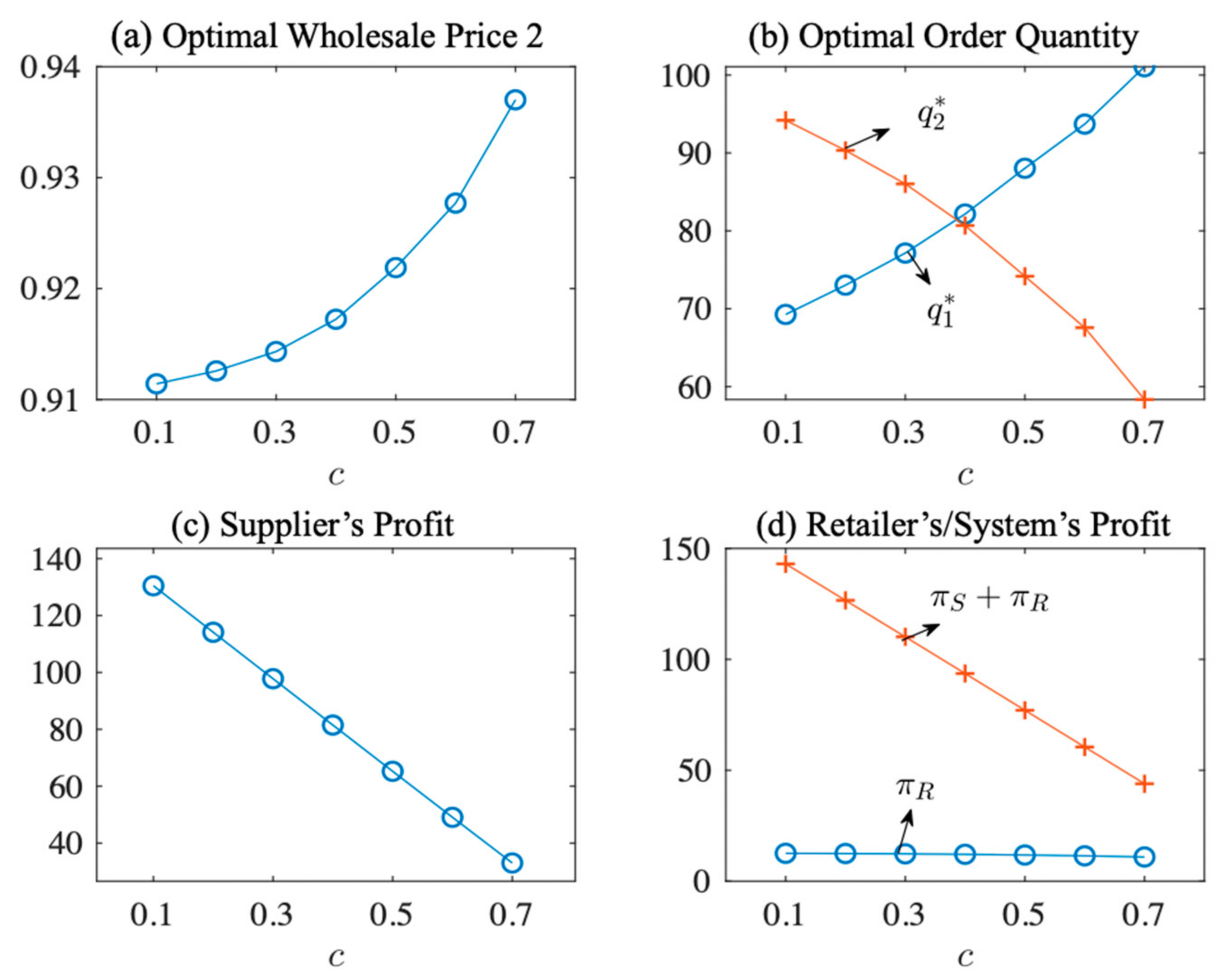
4.4.4. Impact of the Manufacturing Cost

As $c$ increases, the expected loss for the supplier increases. Therefore, as $c$ increases, the supplier increases $w_2^{\mathrm{*}}$ to obtain compensation from her unit inventory income and TC2 becomes more expensive, as shown in Figure 8. Therefore, the retailer increases $q_1^{\mathrm{*}}$ and decreases $q_2^{\mathrm{*}}$.

While the marginal costs of the supplier and retailer increase, the marginal income of the retailer remains unchanged, so the overall supply chain’s profit declines.

4.5. Results and Discussion

This section discusses the above results. In this chapter, we first explore the optimal operation decisions of the capital-constrained retailer and the pricing decisions of the supplier under the two single-trade-credit models. Then, we further investigate the supply chain members’ strategies under the trade credit portfolio.

Through mathematical modelling methods and numerical verification, we have the following findings: (1) Whether under single or mixed trade credit types, the retailer’s optimal profit is determined by the equality of marginal cost and marginal profit across channels. This suggests that the retailer, when faced with multiple financing channels, always starts lending from the channel with the lower marginal cost and ends up with a financing outcome that maintains the same expected cost across financing. (2) The supplier gains a determined revenue under the single-TC1 mode, and takes all the retailer’s profit under the single-TC2 mode. (3) When the retailer uses both TC1 and TC2, the early-payment discount is usually lower than the financing cost of insufficient emergency liquidity. This conclusion is in contrast to Yang and Birge [1], since the bank loan is an uncertain event in this model, while their work requires the retailer to borrow money from the bank at the beginning of the medium term. (4) There is no absolute predominance between the different financing models under different supplier pricing.

5. Conclusions and Discussion

This paper discusses the application and effects of multiple trade credit types in a supply chain. We find that when the bank interest rate is sufficiently low, a capital-constrained retailer uses bank loans as a tool to transfer risk and orders more inventory than a capital-abundant retailer. Under the TCP mode, the early-payment discount is strictly lower than the bank interest rate on emergency loans. Numerical analysis shows that as the proportion of default risk shouldered by the supplier increases, her profit also increases. When the supplier undertakes all of the retailer’s default risk, which implies that the retailer receives no bank credit, the supplier takes all of the sales revenue.

We make the following managerial insights: (1) when the bank interest rate is sufficiently low, the retailer should opt for single-TC1 instead of using TC2; (2) the supplier can participate in the income distribution after the end of the last sales period by providing TC2, which will lead to higher expected profits compared with providing TC1.

These findings contribute to the supply chain financing literature by demonstrating the intricate interplay between different trade credit types and operational decisions in a newsvendor context. We highlight the importance of considering the retailer’s financial constraints and the supplier’s risk management strategies when designing optimal trade credit policies.

Our findings are subject to certain boundary conditions. To simplify the numerical experiment, we employed fixed financial parameters and assumed that market demand follows a bivariate normal distribution. Additionally, we considered a monopoly supplier scenario. However, in reality, markets are competitive, and suppliers engage in horizontal competition. In such cases, instead of maximizing their share of the retailer’s profits, suppliers may lower prices to capture the retailer’s entire order. This could result in lower total profits for competitive suppliers compared to a monopoly supplier, but potentially higher profits for the retailer, thereby improving overall supply chain performance. In addition to this, we assume that the retailer has no working capital. Even with limited capital, retailers often have some initial funds and may opt to self-finance smaller purchases rather than taking out loans. This behavior could be incorporated into future models. Future work could explore the effect of competition between retailers on the financing results. Additionally, our current model assumes a perishable product with zero salvage value, mirroring the classic newsvendor framework. Future work could broaden this model’s applicability to various products and industries. Another promising avenue is to explore the role of trade credit in multi-period settings with stochastic demand.

References

1. Yang, S.A.; Birge, J.R. Trade credit, risk sharing, and inventory financing portfolios. Manag. Sci. 2018, 64, 3667–3689. [Google Scholar] [CrossRef]
2. Cunat, V. Trade credit: Suppliers as debt collectors and insurance providers. Rev. Financ. Stud. 2007, 20, 491–527. [Google Scholar] [CrossRef]
3. Gupta, D.; Wang, L.A. Stochastic inventory model with trade credit. Manuf. Serv. Oper. Manag. 2009, 11, 4–18. [Google Scholar] [CrossRef]
4. Kouvelis, P.; Zhao, W. Financing the newsvendor: Supplier vs. bank, and the structure of optimal trade credit contracts. Oper. Res. 2012, 60, 566–580. [Google Scholar] [CrossRef]
5. Babich, V.; Tang, C.S. Managing opportunistic supplier product adulteration: Deferred payments, inspection, and combined mechanisms. Manuf. Serv. Oper. Manag. 2012, 14, 301–314. [Google Scholar] [CrossRef]
6. Rui, H.; Lai, G. Sourcing with deferred payment and inspection under supplier product adulteration risk. Prod. Oper. Manag. 2015, 24, 934–946. [Google Scholar] [CrossRef]
7. Hu, M.; Qian, Q.; Yang, S.A. Financial Pooling in a Supply Chain; University of Toronto: Toronto, ON, Canada, 2018. [Google Scholar]
8. Chod, J.; Lyandres, E.; Yang, S.A. Trade credit and supplier competition. J. Financ. Econ. 2019, 131, 484–505. [Google Scholar] [CrossRef]
9. Jing, B.; Chen, X.; Cai, G. Equilibrium financing in a distribution channel with capital constraint. Prod. Oper. Manag. 2012, 21, 1090–1101. [Google Scholar] [CrossRef]
10. Beranek, W. Financial implications of lot–size inventory models. Manag. Sci. 1967, 13, B401–B408. [Google Scholar] [CrossRef]
11. Archibald, T.W.; Thomas, L.C.; Betts, J.M.; Johnston, R.B. Should start-up companies be cautious? Inventory policies which maximize survival probabilities. Manag. Sci. 2002, 48, 1161–1174. [Google Scholar] [CrossRef]
12. Li, L.; Shubik, M.; Sobel, M.J. Control of dividends, capital subscriptions, and physical inventories. Manag. Sci. 2013, 59, 1107–1124. [Google Scholar] [CrossRef]
13. Lai, G.; Debo, L.G.; Sycara, K. Sharing inventory risk in supply chain: The implication of financial constraint. Omega 2009, 37, 811–825. [Google Scholar] [CrossRef]
14. Luo, W.; Shang, K. Joint inventory and cash management for multidivisional supply chains. Oper. Res. 2015, 63, 1098–1116. [Google Scholar] [CrossRef]
15. Buzacott, J.A.; Zhang, R.Q. Inventory management with asset-based financing. Manag. Sci. 2004, 50, 1274–1292. [Google Scholar] [CrossRef]
16. Xu, X.; Birge, J.R. Equity valuation, production, and financial planning: A stochastic programming approach. Nav. Res. Logist. 2006, 53, 641–655. [Google Scholar] [CrossRef]
17. Gaur, V.; Seshadri, S. Hedging inventory risk through market instruments. Manuf. Serv. Oper. Manag. 2005, 7, 103–120. [Google Scholar] [CrossRef]
18. Caldentey, R.; Haugh, M. Optimal control and hedging of operations in the presence of financial markets. Math. Oper. Res. 2006, 31, 285–304. [Google Scholar] [CrossRef]
19. Alan, Y.; Gaur, V. Operational investment and capital structure under asset-based lending. Manuf. Serv. Oper. Manag. 2018, 20, 601–800. [Google Scholar] [CrossRef]
20. Babich, V.; Kouvelis, P. Introduction to the Special Issue on Research at the Interface of Finance, Operations, and Risk Management (iFORM): Recent Contributions and Future Directions. Manuf. Serv. Oper. Manag. 2018, 20, 1–18. [Google Scholar] [CrossRef]
21. Silaghi, F.; Moraux, F. Trade credit contracts: Design and regulation. Eur. J. Oper. Res. 2022, 296, 980–992. [Google Scholar] [CrossRef]
22. Haley, C.W.; Higgins, R.C. Inventory policy and trade credit financing. Manag. Sci. 1973, 20, 464–471. [Google Scholar] [CrossRef]
23. An, S.; Li, B.; Song, D.; Chen, X. Green credit financing versus trade credit financing in a supply chain with carbon emission limits. Eur. J. Oper. Res. 2021, 292, 125–142. [Google Scholar] [CrossRef]
24. Ning, J. Strategic trade credit in a supply chain with buyer competition. Manuf. Serv. Oper. Manag. 2022, 24, 2183–2201. [Google Scholar] [CrossRef]
25. Esenduran, G.; Gray, J.V.; Tan, B. A dynamic analysis of supply chain risk management and extended payment terms. Prod. Oper. Manag. 2022, 31, 1394–1417. [Google Scholar] [CrossRef]
26. Park, S.; Ho Yoo, S. Government intervention in environmental performance considering working capital issues: Control the supplier or the buyer? Comput. Ind. Eng. 2022, 163, 107790. [Google Scholar] [CrossRef]
27. Wu, C.; Xu, C.; Zhao, Q.; Zhu, J. Research on financing strategy under the integration of green supply chain and blockchain technology. Comput. Ind. Eng. 2023, 184, 109598. [Google Scholar] [CrossRef]
28. Du, N.; Yan, Y.; Qin, Z. Analysis of financing strategy in coopetition supply chain with opportunity cost. Eur. J. Oper. Res. 2023, 305, 85–100. [Google Scholar] [CrossRef]
29. Yan, N.N.; He, X.L. Optimal trade credit with deferred payment and multiple decision attributes in supply chain finance. Comput. Ind. Eng. 2020, 147, 106627. [Google Scholar] [CrossRef]
30. Christopher, J.; Chen, N.J.; Yang, S.A. The impact of trade credit provision on retail inventory: An empirical investigation using synthetic controls. Manag. Sci. 2022, 69, 4591–4608. [Google Scholar]
31. Wang, J.; Wang, K.; Li, X.; Zhao, R. Suppliers’ trade credit strategies with transparent credit ratings: Null, exclusive, and nonchalant provision. Eur. J. Oper. Res. 2022, 297, 153–163. [Google Scholar] [CrossRef]
32. Babich, V.; Aydin, G.; Brunet, P.Y. Risk, financing and the optimal number of suppliers. In Supply Chain Disruptions; Springer: London, UK, 2012; pp. 195–240. [Google Scholar]
33. Reindorp, M.; Tanrisever, F.; Lange, A. Purchase order financing: Credit, commitment, and supply chain consequences. Oper. Res. 2018, 66, 1287–1303. [Google Scholar] [CrossRef]
34. Cachon, G.P. The allocation of inventory risk in a supply chain: Push, pull, and advance-purchase discount contracts. Manag. Sci. 2004, 50, 222–238. [Google Scholar] [CrossRef]
35. Chod, J. Inventory, risk shifting, and trade credit. Manag. Sci. 2017, 63, 3147–3529. [Google Scholar] [CrossRef]
36. Wang, Z.H.; Qi, L.; Zhang, Y.; Liu, Z. A trade-credit-based incentive mechanism for a risk-averse retailer with private information. Comput. Ind. Eng. 2021, 154, 107101. [Google Scholar] [CrossRef]
37. Yang, H.; Zhuo, W.; Shao, L.; Talluri, S. Mean-variance analysis of wholesale price contracts with a capital-constrained retailer: Trade credit financing vs. bank credit financing. Eur. J. Oper. Res. 2021, 294, 525–542. [Google Scholar] [CrossRef]
38. Zhu, Q.; Wang, C.; Zhang, B. Impact of Capital Position and Financing Strategies on Encroachment in Supply Chain Dynamics. Mathematics 2024, 12, 1830. [Google Scholar] [CrossRef]
39. Schwartz, R.A. An economic model of trade credit. J. Financ. Quant. Anal. 1974, 9, 643. [Google Scholar] [CrossRef]
40. Peura, H.; Yang, S.A.; Lai, G. Trade credit in competition: A horizontal benefit. Manuf. Serv. Oper. Manag. 2017, 19, 263–289. [Google Scholar] [CrossRef]
Figure 1. The sequence of events.
Mathematics 13 01464 g001
Figure 2. The supplier’s profit under different w 1 and r t .
Mathematics 13 01464 g002
Figure 3. Comparison of w 1 and w 2 under different financing modes.
Mathematics 13 01464 g003
Figure 4. Comparison of the optimal order quantity under different financing modes.
Mathematics 13 01464 g004
Figure 5. Comparison of the parties’ profit under different financing modes.
Mathematics 13 01464 g005
Figure 6. Comparison of profits of the overall supply chain under different financing modes.
Mathematics 13 01464 g006
Figure 7. The impact of the bank interest rate.
Mathematics 13 01464 g007
Figure 8. The impact of the manufacturing cost.
Mathematics 13 01464 g008