Abstract
The Multiscale Geographically and Temporally Weighted Regression model overcomes the limitation of estimating spatiotemporal variation characteristics of regression coefficients for different variables under a single scale, making it a powerful tool for exploring the spatiotemporal scale characteristics of regression relationships. Currently, the most widely used estimation method for multiscale spatiotemporal geographically weighted models is the backfitting-based iterative approach. However, the iterative process of this method leads to a substantial computational burden and the accumulation of errors during iteration. This paper proposes a non-iterative estimation method for the MGTWR model, combining local linear fitting and two-step weighted least squares estimation techniques. Initially, a reduced bandwidth is used to fit a local linear GTWR model to obtain the initial estimates. Then, for each covariate, the optimal bandwidth and regression coefficients are estimated by substituting the initial estimates into a localized least squares problem. Simulation experiments are conducted to evaluate the performance of the proposed non-iterative method compared to traditional methods and the backfitting-based approach in terms of coefficient estimation accuracy and computational efficiency. The results demonstrate that the non-iterative estimation method for MGTWR significantly enhances computational efficiency while effectively capturing the scale effects of spatiotemporal variation in the regression coefficient functions for each predictor.
Keywords:
multiscale GTWR; local linear estimator; spatiotemporal non-stationarity; spatiotemporal regression; nonparametric estimation MSC:
62G05
1. Introduction
Brunsdon and Fotheringham et al. (1996) [1] proposed the Geographically Weighted Regression (GWR) model, which allows the relationship between the response variable and covariates to vary spatially. This model has been widely applied in disciplines such as geography [2], economics [3], epidemiology [4], meteorology [5], and environmental science [6]. However, classical GWR estimation relies on locally weighted least squares estimation, assuming that all modeling processes operate at the same spatial scale and thereby neglecting scale differences in spatial relationships. Scale is a critical concept in geography [7,8]. To quantify and identify multiscale processes in modeling, Fotheringham et al. (2017) [9] proposed a multiscale extension of GWR, termed Multiscale Geographically Weighted Regression (MGWR). This framework relaxes the single-bandwidth constraint in GWR and permits relationships between the response variable and covariates to vary across distinct spatial scales. Subsequently, many studies have provided effective extensions for the development of MGWR (Lu et al. (2017) [10], Lu et al. (2018) [11], Yu et al. (2020) [12], Wei et al. (2012) [13], Comber et al. (2023)) [14].
In order to consider the influence of time factors, Huang et al. (2010) [15] introduced the Geographically and Temporally Weighted Regression (GTWR) model, which introduces time effects through a new spatiotemporal kernel function. Fotheringham et al. (2015) [16] further extended GWR to spatiotemporal data by redesigning the spatiotemporal weighting matrix and modifying the selection of optimal spatial and temporal bandwidth. However, these two GTWR models still cannot independently identify the scale characteristics of the regression relationship between the dependent variable and the independent variable. Incorporating temporal factors into the multiscale model for consideration, Wu et al. (2019) [17] extended multiscale GTWR by specifying flexible bandwidths for covariates, enabling a versatile framework for analyzing multiscale spatiotemporal processes. Zhang and Mei et al. (2021) [18] proposed a one-sided temporally weighted GTWR (UGTWR) model and its multiscale extension (MUGTWR), which employs an iterative backfitting algorithm to assign distinct bandwidths to coefficients with heterogeneous spatiotemporal scales. Hong et al. (2025) [19] generalized the GTWR framework to MGTWR by redefining it as a GAM [20] and deriving local coefficient standard errors for nonstationarity testing. However, the multiscale nature of MGWR [9] and MGTWR [17] incurs substantial computational costs. Conventional estimation methods treat these models as GAMs and use backfitting algorithms to estimate coefficient surfaces. Currently, MGWR is computationally feasible only for small datasets, while medium-sized datasets (>5000 observations) demand prohibitive runtime [21]; incorporating temporal dimensions further escalates computational burdens.
To address efficiency challenges, Oshan et al. (2019) [22] developed a Python-based MGWR implementation with enhanced diagnostics and computational performance. Li et al. (2020) [21] proposed a parallelized MGWR estimation method, reducing memory usage and runtime to enable applications on medium to large datasets (up to 100,000 observations). Murakami et al. (2020) [23] introduced Scalable GWR (ScaGWR), which optimizes matrix–vector precompression and leave-one-out cross-validation to calibrate models with up to 1 million observations without parallelization. Zhou et al. (2023) [24] proposed a gradient-based MGWR estimation method by deriving gradients and Hessian matrices of the corrected Akaike Information Criterion (AICc) and employing trust-region optimization, yielding significant computational gains for large samples but lacking temporal integration. Wu et al. (2022) [25] proposed a local linear-fitting-based MGWR (MGWR-LL), which models coefficients as spatially varying linear functions with distinct smoothness, estimated via a two-step least squares algorithm. MGWR-LL outperforms conventional MGWR in goodness of fit, bias reduction, and computational efficiency, particularly for large datasets. Despite these advances, achieving computational efficiency and estimation accuracy for MGTWR remains a significant challenge.
Compared with GWR, GTWR, and MGWR models, although the MGTWR model has made significant improvements, it still has limitations. To date, the most widely used estimation method for MGTWR models is the iterative method based on inverse fitting. However, the iterative process of this method may result in a significant computational burden and accumulation of errors during the iteration process. The key limitation of the MGTWR model lies in how to effectively explore the spatiotemporal scale effects of complex data while improving computational speed. Finally, this study integrates local linear fitting [26] and two-step weighted least squares estimation [27] to propose a non-iterative estimation method for MGTWR. Firstly, we use a narrow bandwidth to fit the local linear GTWR model for initial estimation. For each covariate, the optimal bandwidth and coefficient function can be obtained by substituting the initial estimate into the local least squares problem. This method does not require repeated iterations and only needs to traverse all variables for univariate estimation during the multiscale estimation stage to obtain the optimal estimate. This method improves computational efficiency by two-thirds compared to the traditional MGTWR-BF model, corrects boundary effects in coefficient estimation, and demonstrates superiority in explaining spatiotemporal effects and scale heterogeneity among covariates.
The rest of this article is organized as follows. Section 2 briefly reviews the MGTWR model. Section 3 provides a brief review of the MGTWR model estimation method based on the backfitting algorithm. In Section 4, the 2SLS estimation method based on GTWR is derived, and its local linear GTWR version is also derived, forming the MGTWR-LL estimation method. On this basis, Section 5 conducts simulation studies to evaluate and compare the performance of the MGTWR-LL estimation method in the MGTWR model. The article ends with a conclusion and discussion.
2. Multiscale Geographically and Temporally Weighted Regression Model
The MGTWR model can be expressed as follows:
where represents the spatiotemporal position, where the spatial vertical axis is , the spatial horizontal axis is , and the temporal axis is . and represent the response variable and independent variable, respectively, at the spatiotemporal location . is the intercept term of the regression relationship, and represents the regression coefficient of the -th independent variable at the spatiotemporal position . is an independent random error term. is the spatiotemporal bandwidth derived for the -th regression relationship based on the specific temporal bandwidth and spatial bandwidth .
3. Back-Fitting Algorithms Based on Multiscale Geographically and Temporally Weighted Regression Model
The estimation method of the multiscale GTWR model based on backfitting is a widely used estimation approach for multiscale models. By treating the product of the regression coefficients and independent variables as an additive term, the model is written in the form of a Generalized Additive Model (GAM) as follows:
where and .
The algorithm for the backfitting-based MGTWR model is as follows:
(1) Initialize the estimation for each additive term , , , …, , where “⊗” represents element-wise multiplication of two vectors, and denote the initial estimates as . Compute the initial residuals as .
(2) Add the computed initial residuals to the first initial term and use the GTWR model to regress on (using the identity matrix I for the intercept term). This provides the optimal spatial bandwidth and temporal bandwidth for the first covariate, as well as a set of updated local estimates. Update the first additive term , and update the residuals .
(3) Use the updated residuals from step (2), add , and regress on to obtain the optimal spatial bandwidth and temporal bandwidth for the second covariate. Update the residuals as .
(4) Perform regression for each term corresponding to its respective variable, continuing until the bandwidths and coefficient function estimates for the last variable are determined, completing the first iteration.
(5) Continue iterating until the convergence criterion is met, at which point the iteration stops.
The termination criterion for the backfitting iteration in the MGTWR model is that, after convergence, the difference between consecutive iterations (referred to as the change score, SOC) is sufficiently small, and there are two SOC options to choose from:
1. The change in the ratio of the residual squared sum to RSS is denoted as :
2. The change in GTWR smoothness is denoted as :
where both and are unitless indicators. In this paper, the iteration process uses as the termination criterion for the backfitting process in the MGTWR model.
The computational efficiency of MGTWR mainly depends on the initial estimated values of the parameters in the first step. We obtain the estimated parameters of GTWR through an independent backfitting process (setting a relatively loose threshold , and we use it as the initial value of MGTWR while defining a stricter convergence threshold for MGTWR calibration.
4. Local-Linear-Fitting-Based Multiscale Geographically and Temporally Weighted Regression Model
Firstly, we obtain an initial estimate based on the local linear GTWR model.
To simplify the notation, we rewrite Equation (1) as follows:
where, by assuming , the model can include spatiotemporally varying intercept terms. Let each coefficient function (for ) have continuous partial derivatives concerning the spatiotemporal coordinates u, , and t. Given the point , for each , by Taylor’s theorem, in Equation (5) can be approximated by a linear function of u, v, and t in the neighborhood of , i.e.,
where , , and are the partial derivatives of with respect to u, v, and t evaluated at . To estimate the unknown parameters , , , and for , the following optimization problem is solved:
This expression is minimized, where , are the observed values of the dependent variable Y and the independent variables at the spatiotemporal location , while is the weight function, .
The selection of bandwidth is crucial for the estimation of the model. This article uses the modified Akaike information criterion (AICc) to select the optimal temporal bandwidth and spatial bandwidth. The expression for AICc is as follows:
where n is the sample size, is the estimated standard deviation of the error term, L is the hat matrix, and the bandwidth that minimizes the AICc value is the optimal temporal bandwidth and spatial bandwidth.
For spatial distance and temporal distance , the weight is defined as follows:
Simplifying the expression, the kernel functions are given as follows:
where and represent the spatial and temporal bandwidths, respectively. The bi-square kernel function exhibits special advantages in local polynomial regression: its derivative continuity makes it more stable in variable bandwidth selection and satisfies the optimal adaptability condition for Donoho–Johnstone threshold selection.
Let
The solution to the least squares problem can be expressed as follows:
Therefore
where is a -dimensional row vector with the th element equal to 1 and all other elements equal to 0.
Taking for , the estimated coefficient function vector at each observation location is given by the following:
where D is a matrix defined as follows:
where is a -dimensional row vector with the th element equal to 1 and all other elements equal to 0.
Thus, the fitted values of the dependent variable Y at the observation locations are given by the following:
where is the column vector of the observed values of the independent variables for the ith sample.
Then, based on the initial estimation, multiscale estimation results are obtained.
Since the first step only provides a suboptimal estimate, the second step refines the bandwidth and coefficients. For each covariate, such as , its final bandwidth and corresponding regression coefficient need to be re-estimated by substituting the initial estimates into a local least squares problem (i.e., minimizing):
where represents the temporal bandwidth and spatial bandwidth to be optimized. It can be seen that, except for , , and , the other coefficients are predetermined in the first step, and the above least squares problem becomes a univariate minimization problem. Therefore, the optimal bandwidth and its related coefficients can be obtained as follows:
where
and
The basic steps of MGTWR-LL are as follows:
(i) The GTWR model is estimated using a local linear fitting method, and an optimal spatial bandwidth and an optimal temporal bandwidth are selected based on the AICc criterion.
(ii) Let , , where and c is called the bandwidth reduction factor. This reduces the bandwidths selected in (i). Under and , all coefficients , where , are estimated using weighted least squares at the points . The estimated values are given by the following:
(iii) For each covariate, the bandwidth and associated coefficients are refined in an ordered manner. The following operation is performed for m from 1 to p:
For , regression is performed on , and the final estimate of the mth coefficient at each sample point is as follows:
where
5. Numerical Simulation
Subsequently, the performance of the MGTWR-LL model was validated through simulation experiments. The simulated data for the study area are located within a rectangle with both length and width equal to 1. The sampling points are arranged in an grid. Here, and , and so the total number of samples is . The spatiotemporal locations of the samples are calculated as follows:
where and represent the remainder and integer part, respectively, of a divided by b.
The data generation process can be described as follows:
where y is the dependent variable; and are independent variables randomly drawn from the normal distribution ; and is the independent error term, following the normal distribution .
To assess the performance of the GTWR method under different regression coefficient complexities, the coefficients are defined to exhibit varying levels of spatiotemporal heterogeneity, as follows:
In order to compare the consistency of GTWR, MGTWR-BF, and the proposed MGTWR-LL, all estimation processes in these three GTWR methods use a bi-square kernel function to generate weights, and the AICc criterion is employed to select the optimal spatial bandwidth and the optimal temporal bandwidth.
Considering the randomness in data generation, the simulation experiment was repeated times. Additionally, we used the Root Mean Square Error (RMSE) and Mean Absolute Error (MAE) to evaluate the accuracy of the estimates.
Furthermore, the average RMSE and MAE across the N repeated experiments are used to measure the accuracy of the estimates:
At the same time, the Residual Sum of Squares (RSS) and goodness-of-fit measure are used to compare the five estimation methods of the GTWR models. We perform comparative experiments designed to compare the effectiveness of the method proposed in this paper. The five methods are the classical spatiotemporal geographically weighted regression model (GTWR), the spatiotemporal geographically weighted regression model based on local linear fitting (GTWRLP), the multiscale spatiotemporal geographically weighted regression model based on backfitting (MGTWR-BF), the multiscale spatiotemporal geographically weighted regression model with backfitting and local linear fitting (MGTWRLP-BF), and the non-iterative multiscale spatiotemporal geographically weighted regression model proposed in this paper (MGTWR-LL). The average RSS (ARSS) and average (AR2) represent the mean values of the RSS and for the N repetitions conducted in the evaluation.
As shown in Table 1, the MGTWR-LL model has the lowest ARMSE, AMAE, and AAICc values among the models, indicating that its predicted values have minimal deviation from the true values, with errors significantly lower than those of other methods. The non-iterative local linear method dynamically adjusts local weights through bandwidth, enabling more flexible capture of nonlinear relationships in the data, thereby reducing global bias. The value of the MGTWR-LL model is 0.9900, demonstrating its strong explanatory power. The model achieves optimal parameter complexity control while maintaining high accuracy, avoiding the risk of overfitting and providing the most accurate fit. The MGTWR-LL model performs excellently overall, especially in terms of model complexity, residuals, and goodness of fit, making it suitable for applications that require high predictive accuracy and model simplicity.

Table 1.
The ARMSE, AMAE, , ARSS, and AAICc of the GTWR, GTWRLP, MGTWR-BF, MGTWRLP-BF, and MGTWR-LL methods across 500 simulation repetitions.
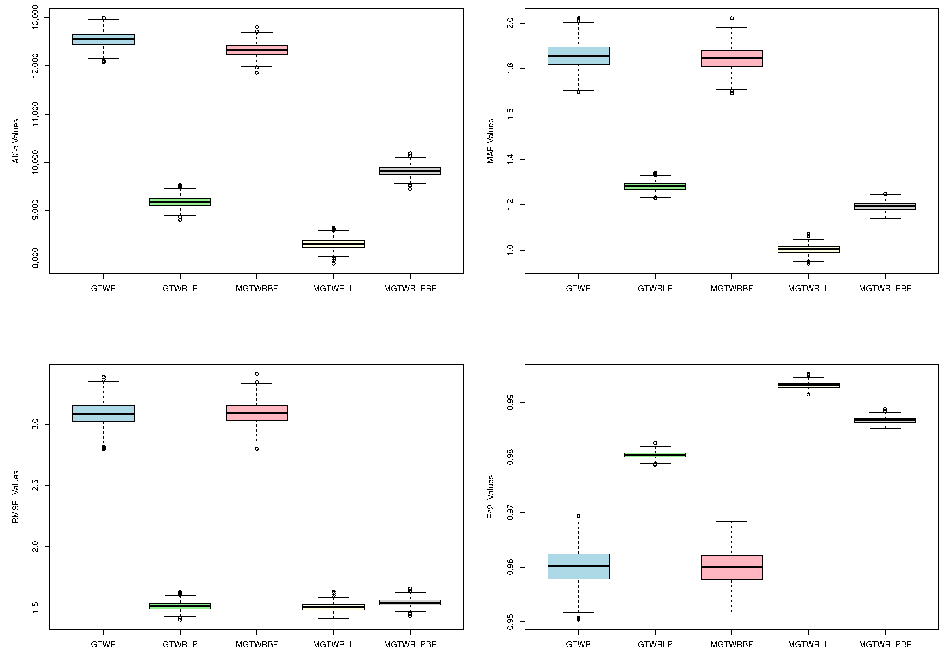
As shown in Figure 1, the box plots of various model metrics across 500 repeated experiments indicate that for the MGTWR-LL model, the AICc value is relatively small (positioned relatively low), suggesting that it performs better in model selection, with lower overall complexity than other models (such as GTWR and GTWRLP). This indicates its greater effectiveness in model fitting, avoiding the risk of overfitting. The value box is relatively high, with its distribution concentrated near 1, which highlights the model’s superiority in fitting the data and capturing spatiotemporal heterogeneity. The MAE value of the model is distributed in a lower range, with a short box and a lower position, indicating the lowest average absolute error in its predictions. Compared to other models (such as MGTWR-BF and MGTWRLP-BF), it has reduced prediction biases, demonstrating superior performance. The RMSE value box for the MGTWR-LL model is positioned lower with a shorter box length, indicating the smallest root mean square error, meaning that the difference between predicted and actual values is minimized, reflecting superior accuracy. Overall, the MGTWR-LL method demonstrates superior performance in both reducing bias and increasing accuracy.
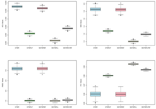
Figure 1.
Box plots of AICc, MAE, RMSE, and for the MGTWR-LL model across 500 repeated experiments with .
In order to compare the impact of different estimation methods on the accuracy of coefficient function estimation, N repeated experiments were conducted for each estimation method. represents the estimate of the kth coefficient function at point in the rth experiment. The root mean square error (RMSE) for the estimated coefficient function at point over N experiments is calculated as follows:
where the accuracy of the estimation of the coefficient function is evaluated using the average RMSE over n sampling points:
As shown in Table 2, for the MGTWR-LL method, the MRMSE values are similar and relatively low in the range from to , indicating that the model’s accuracy is high for these values of c. In particular, at , the MRMSE is the lowest, and the model achieves the highest accuracy. Considering both the MRMSE metric and the influence of different bandwidth reduction factors c, the MGTWR-LL method performs best at , achieving optimal estimation accuracy. The estimation accuracy of the coefficient functions shows no significant difference within the bandwidth reduction factor range of to . The estimation accuracy is not sensitive to changes in c within this range, making the choice of c more flexible in practical applications. The accuracy of the estimation method is relatively insensitive to changes in c within this specific range, a feature that facilitates the selection of an appropriate c value in practical operations. The average computation times for each GTWR method across more than 500 repetitions are shown in Table 2. In terms of runtime, MGTWR-LL has higher computational efficiency than other multiscale models. The average runtime for MGTWR-LL is 44 s, reflecting a significant improvement in computation speed and saved computational time. In summary, the MGTWR-LL method is more applicable and feasible.
Table 2.
MRMSE and average computation time for each coefficient function estimate across repeated experiments.
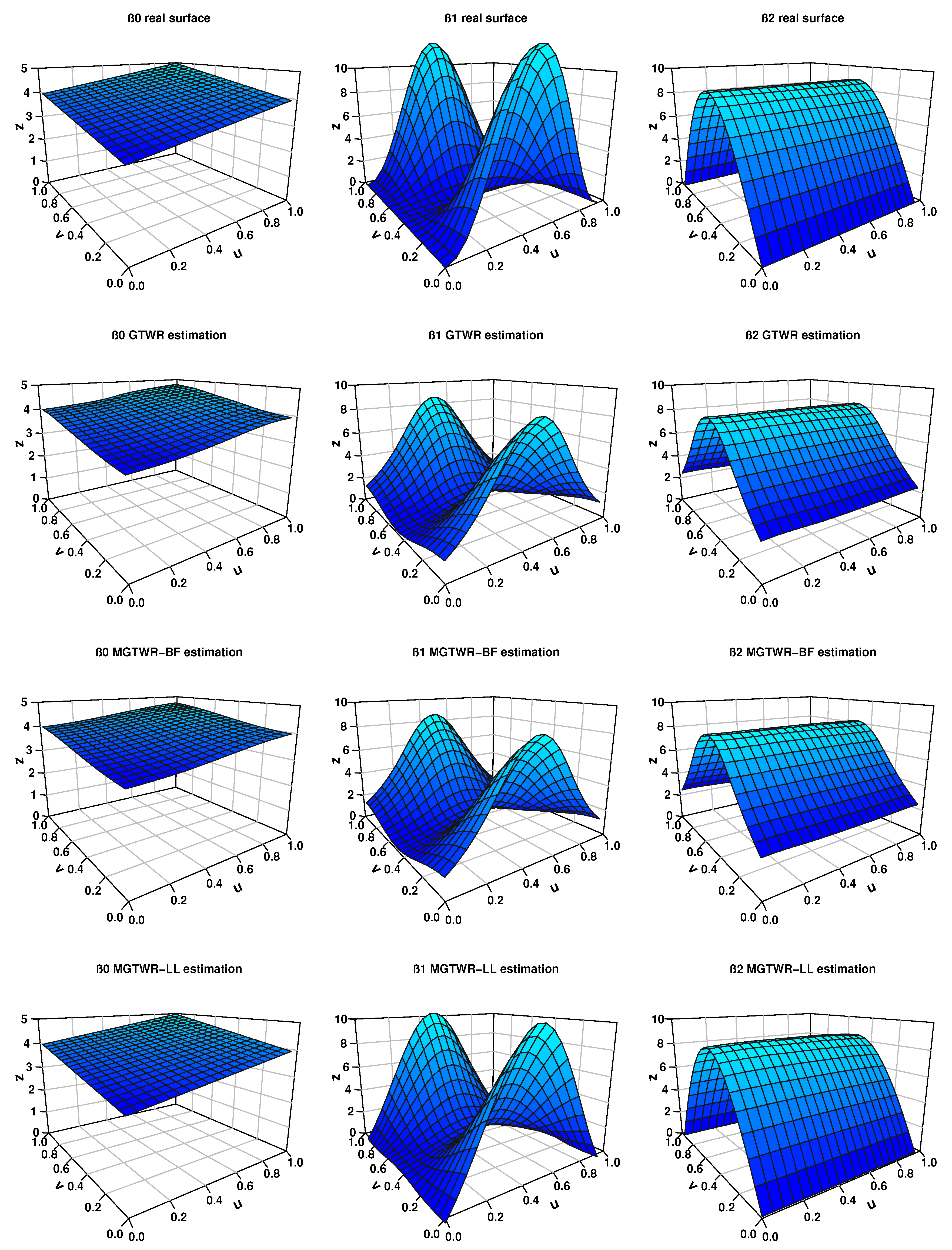
To demonstrate the ability of different methods to estimate coefficient surfaces, Figure 2 uses the averages from 100 repeated experiments as the estimated coefficient surfaces for comparison. The estimated surfaces obtained from GTWR, MGTWR-BF, and MGTWR-LL are compared with the true surface. All estimated surfaces are similar to the actual surface, indicating that they are effective models for capturing spatial heterogeneity. However, there are certain biases at the boundaries when compared to the true surface. MGTWR-LL is closer to the true surface at the boundaries, suggesting that this method has the potential to automatically correct boundary effects. Overall, the simulation results indicate that the MGTWR-LL method demonstrates satisfactory performance in terms of estimation accuracy. The GTWR fitting method is essentially a form of the Nadaraya–Watson kernel estimation method. The Nadaraya–Watson kernel estimation method has boundary effects. However, for spatiotemporal coefficient models, since the coefficient function is a ternary function of spatiotemporal geographic coordinates, the boundary part of the three-dimensional geographic area is much larger than that of the one-dimensional interval. Therefore, the boundary effects of the GTWR method will be more severe. This severe boundary effect can lead to significant distortion in the estimation of coefficient functions in the boundary region, resulting in inaccurate analysis results. Considering that the local polynomial fitting method has many advantages such as automatic correction of boundary effects, this paper extends the local linear GWR method proposed by Wang et al. (2008) [26] to spatiotemporal space, which expands the coefficient function locally into a linear function of spatiotemporal geographic coordinates, and then uses the GTWR fitting method to estimate the coefficient function, which can effectively correct boundary effects.
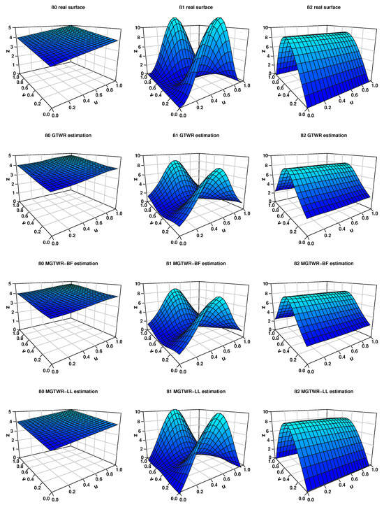
Figure 2.
For , the average surfaces of the three coefficient functions from 100 repeated simulation experiments under three estimation methods (GTWR, MGTWR-LL, and MGTWR-BF) are shown. The first, second, and third columns are the coefficient surfaces , , and . The first row contains the true surfaces of , , and . The second row shows the GTWR-estimated surfaces, the third row shows the MGTWR-BF-estimated surfaces, and the fourth row displays the MGTWR-LL-estimated surfaces.
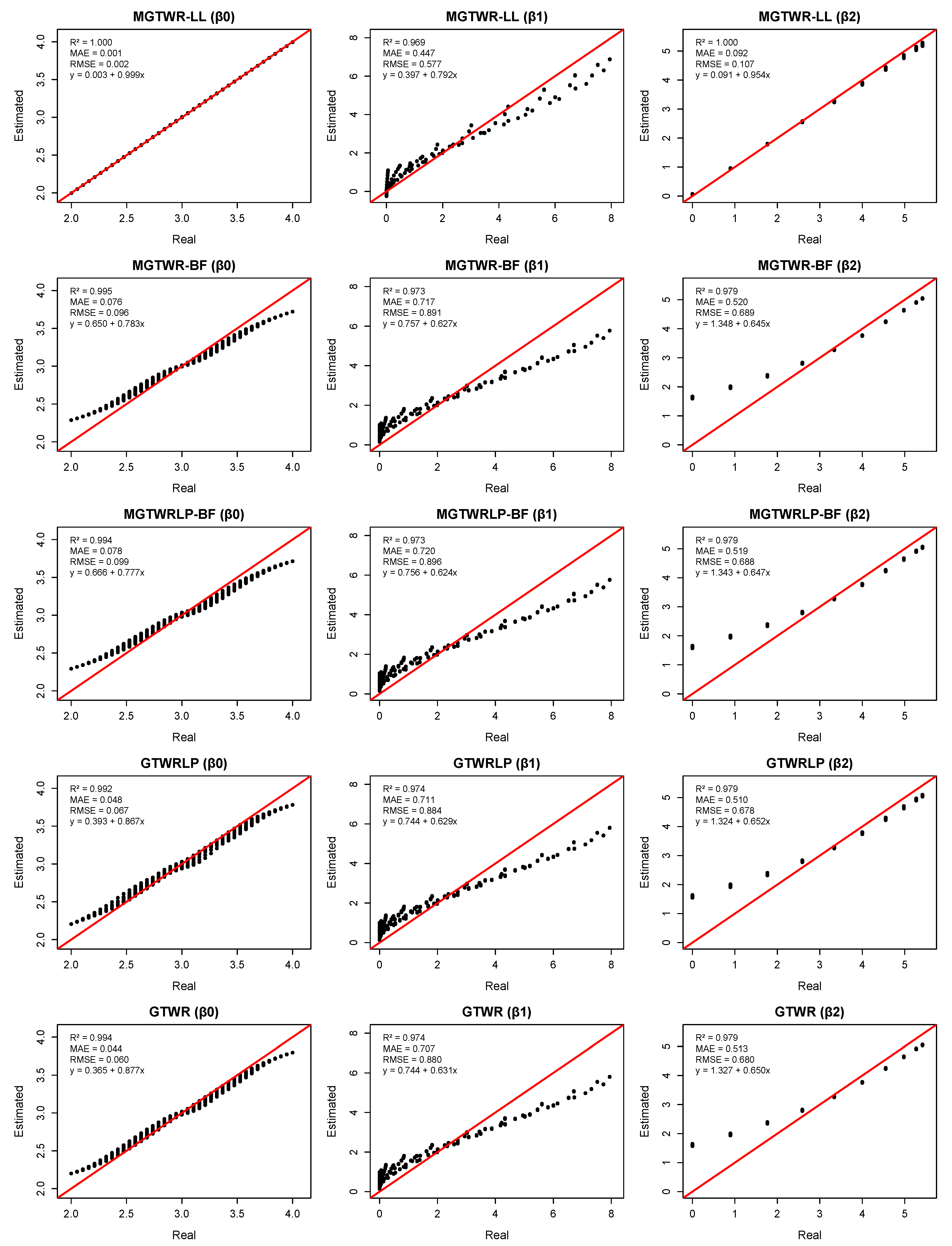
Furthermore, to visually demonstrate the accuracy of coefficient estimates at each location, scatter plots of the true values and estimated values for the five estimation methods are presented. For the MGTWR-LL method in Figure 3, at , the values between the true and estimated values for , , and are 1.000, 0.969, and 1.000, respectively. It can be observed that the non-iterative method provides excellent fit, indicating that the method has low estimation bias and high estimation accuracy. The estimated points for the MGTWR-LL method are almost entirely clustered along the diagonal, suggesting that the dispersion between the estimated values and true values is very small, with low volatility and high reliability. Especially for and , almost all points are concentrated around the diagonal. From a column perspective, this multiscale method can effectively estimate different coefficient functions, with the fluctuations in the coefficient scatter plots being lower than those of other methods. The experiment shows that the MGTWR-LL method is suitable for modeling datasets with spatiotemporal heterogeneity, and its estimation accuracy significantly outperforms that of other models.
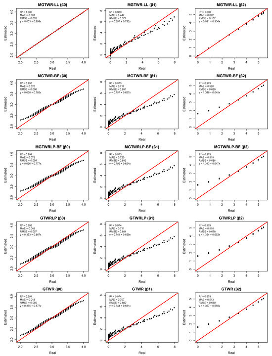
Figure 3.
For , scatter plots of the average three coefficient functions from 100 repeated simulation experiments for GTWR under five estimation methods are shown. The first column compares , the second column compares , and the third column compares . The first row shows the MGTWR-LL estimation results, the second column shows the MGTWR-BF estimation results, the third column shows the MGTWRLP-BF estimation results, the fourth column shows the GTWRLP estimation results, and the fifth column shows the GTWR estimation results.
6. Discussion
The MGTWR model is one of the most useful tools for studying the spatial relationships between variables in multiscale processes. Developing new models to enhance MGTWR remains a challenge under many conditions, such as computational speed, estimation accuracy, and applicability to data. In this study, inspired by the GWR method based on local linearity proposed by Wang et al. [26] and the two-step least squares estimation method proposed by Fan et al. [27], this paper reconstructs the estimation method of the MGTWR model based on the 2SLS estimation of the GTWR model within the framework of local linear polynomial modeling and provides an effective two-step estimation algorithm to estimate the multiscale bandwidth and its correlation coefficients. The simulation experiment results show that the performance of MGTWR-LL is significantly better than that of the backfitting estimation method in terms of computational efficiency and estimating regression coefficients and that it can effectively reveal the spatiotemporal scale of an explanatory variable’s effect.
Through numerical simulation experiments, this paper comprehensively evaluates the performance of the non-iterative estimation method for the multiscale spatiotemporal geographically weighted regression (MGTWR) model in terms of coefficient function estimation accuracy, computational efficiency, and the effectiveness of revealing the spatiotemporal scale of each coefficient function. The following conclusions are drawn:
1. In the simulation experiments, the proposed non-iterative algorithm for the MGTWR model significantly outperforms the backfitting-based MGTWR model and our designed backfitting-based local linear fitting MGTWR estimation method in terms of runtime. Furthermore, based on the results of the simulation experiments, it also significantly improves estimation accuracy and reduces coefficient estimation bias.
2. According to the comparison in the simulation experiments, the non-iterative estimation method of the multiscale spatiotemporal geographically weighted model (MGTWR) not only inherits the advantages of the backfitting iterative method—the ability to independently estimate individual coefficients—but also significantly enhances computational efficiency. Therefore, the non-iterative algorithm proposed for the MGTWR model is an effective method for analyzing the spatiotemporal scale effects of different variable regression coefficients.
In addition, the MGTWR model assumes that all regression coefficients vary in time and space, and its estimation also provides information about the spatiotemporal non-stationarity of the regression coefficients through the variable-specific optimal bandwidth size. Formal statistical tests for identifying constant and variable coefficients for assessing the significance of the effect of explanatory variables at each spatiotemporal sampling point are also essential for local MGTWR modeling in related areas of research. Considering the information on the spatiotemporal non-stationarity of each regression coefficient provided by the MGTWR estimation method as a priori information, the exceptionally large bandwidth size of the regression coefficient implies that the coefficient may be constant, and we can formulate more specific null hypotheses to test for possible constant coefficients in the MGTWR model. After identifying the constant regression coefficients in the MGTWR model, a semiparametric MGTWR model was developed in which some of the regression coefficients are constants and others are spatially varying. In future research, the MGTWR-LL estimation method can be extended to the semiparametric MGTWR model. These issues deserve to be explored in future research. The study suggests that extending this non-iterative estimation method to semiparametric GTWR models and spatiotemporal autoregressive GTWR models is a promising direction for further research. This extension could not only further optimize the computational performance of the model but also provide new solutions for the analysis of complex spatiotemporal data.
Author Contributions
Conceptualization and methodology, H.-G.Z.; software and visualization, Y.-D.D.; writing—original draft preparation, H.-G.Z.; writing—review and editing, H.-G.Z. and Y.-D.D. All authors have read and agreed to the published version of the manuscript.
Funding
This research was funded by the Natural Science Foundation of Xinjiang Uygur Autonomous Region (grant number 2023D01C01) and Humanities and Social Sciences division of the Ministry of Education Planning Fund (grant number 19YJA910007).
Data Availability Statement
All data and their generation processes supporting this study are included in the article.
Acknowledgments
The author sincerely thanks the four reviewers for their valuable comments and constructive suggestions, which have significantly improved the manuscript.
Conflicts of Interest
The authors declare no conflicts of interest.
References
- Brunsdon, C.; Fotheringham, A.S.; Charlton, M.E. Geographically weighted regression: A method for exploring spatial nonstationarity. Geogr. Anal. 1996, 28, 281–298. [Google Scholar] [CrossRef]
- Douglas, E.M.; Vogel, R.M.; Kroll, C.N. Trends in floods and low flows in the United States: Impact of spatial correlation. J. Hydrol. 2000, 240, 90–105. [Google Scholar] [CrossRef]
- Marwal, A.; Silva, E.A. Analysing inequity in accessibility to services with neighbourhood location and socio-economic characteristics in Delhi. Geogr. Anal. 2024, 56, 651–677. [Google Scholar] [CrossRef]
- Sannigrahi, S.; Pilla, F.; Basu, B.; Basu, A.S.; Molter, A. Examining the association between socio-demographic composition and COVID-19 fatalities in the European region using spatial regression approach. Sustain. Cities Soc. 2020, 62, 102418. [Google Scholar] [CrossRef] [PubMed]
- Cao, Z.; Wu, Z.; Li, S.; Guo, G.; Song, S.; Deng, Y.; Ma, W.; Sun, H.; Guan, W. Explicit Spatializing Heat-Exposure Risk and Local Associated Factors by coupling social media data and automatic meteorological station data. Environ. Res. 2020, 188, 109813. [Google Scholar] [CrossRef]
- Zhang, Y.; Yang, Y.; Chen, J.; Shi, M. Spatiotemporal heterogeneity of the relationships between PM2.5 concentrations and their drivers in China’s coastal ports. J. Environ. Manag. 2023, 345, 118698. [Google Scholar] [CrossRef]
- Goodchild, M.F. Models of scale and scales of modelling. In Modelling Scale in Geographical Information Science; John Wiley & Sons: Hoboken, NJ, USA, 2001; pp. 3–10. [Google Scholar]
- Murakami, D.; Lu, B.; Harris, P.; Brunsdon, C.; Charlton, M.; Nakaya, T.; Griffith, D.A. The importance of scale in spatially varying coefficient modeling. Ann. Am. Assoc. Geogr. 2019, 109, 50–70. [Google Scholar] [CrossRef]
- Fotheringham, A.S.; Yang, W.; Kang, W. Multiscale geographically weighted regression (MGWR). Ann. Am. Assoc. Geogr. 2017, 107, 1247–1265. [Google Scholar] [CrossRef]
- Lu, B.; Brunsdon, C.; Charlton, M.; Harris, P. Geographically weighted regression with parameter-specific distance metrics. Int. J. Geogr. Inf. Sci. 2017, 31, 982–998. [Google Scholar] [CrossRef]
- Lu, B.; Yang, W.; Ge, Y.; Harris, P. Improvements to the calibration of a geographically weighted regression with parameter-specific distance metrics and bandwidths. Comput. Environ. Urban Syst. 2018, 71, 41–57. [Google Scholar] [CrossRef]
- Yu, H.; Fotheringham, A.S.; Li, Z.; Oshan, T.; Kang, W.; Wolf, L.J. Inference in multiscale geographically weighted regression. Geogr. Anal. 2020, 52, 87–106. [Google Scholar] [CrossRef]
- Wei, C.H.; Qi, F. On the estimation and testing of mixed geographically weighted regression models. Econ. Model. 2012, 29, 2615–2620. [Google Scholar] [CrossRef]
- Comber, A.; Harris, P.; Brunsdon, C. Multiscale spatially varying coefficient modelling using a Geographical Gaussian Process GAM. Int. J. Geogr. Inf. Sci. 2024, 38, 27–47. [Google Scholar] [CrossRef]
- Huang, B.; Wu, B.; Barry, M. Geographically and temporally weighted regression for modeling spatio-temporal variation in house prices. Int. J. Geogr. Inf. Sci. 2010, 24, 383–401. [Google Scholar] [CrossRef]
- Fotheringham, A.S.; Crespo, R.; Yao, J. Geographical and temporal weighted regression (GTWR). Geogr. Anal. 2015, 47, 431–452. [Google Scholar] [CrossRef]
- Wu, C.; Ren, F.; Hu, W.; Du, Q. Multiscale geographically and temporally weighted regression: Exploring the spatiotemporal determinants of housing prices. Int. J. Geogr. Inf. Sci. 2019, 33, 489–511. [Google Scholar] [CrossRef]
- Zhang, Z.; Li, J.; Fung, T.; Yu, H.; Mei, C.; Leung, Y.; Zhou, Y. Multiscale geographically and temporally weighted regression with a unilateral temporal weighting scheme and its application in the analysis of spatiotemporal characteristics of house prices in Beijing. Int. J. Geogr. Inf. Sci. 2021, 35, 2262–2286. [Google Scholar] [CrossRef]
- Hong, Z.; Wang, R.; Wang, Z.; Du, W. Inference issue in multiscale geographically and temporally weighted regression. Stat. Comput. 2025, 35, 30. [Google Scholar] [CrossRef]
- Hastie, T.; Tibshirani, R. Generalized additive models: Some applications. J. Am. Stat. Assoc. 1987, 82, 371–386. [Google Scholar] [CrossRef]
- Li, Z.; Fotheringham, A.S. Computational improvements to multi-scale geographically weighted regression. Int. J. Geogr. Inf. Sci. 2020, 34, 1378–1397. [Google Scholar] [CrossRef]
- Oshan, T.M.; Li, Z.; Kang, W.; Wolf, L.J.; Fotheringham, A.S. mgwr: A Python implementation of multiscale geographically weighted regression for investigating process spatial heterogeneity and scale. ISPRS Int. J. Geo-Inf. 2019, 8, 269. [Google Scholar] [CrossRef]
- Murakami, D.; Tsutsumida, N.; Yoshida, T.; Nakaya, T.; Lu, B. Scalable GWR: A linear-time algorithm for large-scale geographically weighted regression with polynomial kernels. Ann. Am. Assoc. Geogr. 2020, 111, 459–480. [Google Scholar] [CrossRef]
- Zhou, X.; Assunção, R.; Shao, H.; Huang, C.C.; Janikas, M.; Asefaw, H. Gradient-based optimization for multi-scale geographically weighted regression. Int. J. Geogr. Inf. Sci. 2023, 37, 2101–2128. [Google Scholar] [CrossRef]
- Wu, B.; Yan, J.; Lin, H. A cost-effective algorithm for calibrating multiscale geographically weighted regression models. Int. J. Geogr. Inf. Sci. 2022, 36, 898–917. [Google Scholar] [CrossRef]
- Wang, N.; Mei, C.L.; Yan, X.D. Local linear estimation of spatially varying coefficient models: An improvement on the geographically weighted regression technique. Environ. Plan. A 2008, 40, 986–1005. [Google Scholar] [CrossRef]
- Fan, J.; Zhang, W. Statistical estimation in varying coefficient models. Ann. Stat. 1999, 27, 1491–1518. [Google Scholar] [CrossRef]
Disclaimer/Publisher’s Note: The statements, opinions and data contained in all publications are solely those of the individual author(s) and contributor(s) and not of MDPI and/or the editor(s). MDPI and/or the editor(s) disclaim responsibility for any injury to people or property resulting from any ideas, methods, instructions or products referred to in the content. |
© 2025 by the authors. Licensee MDPI, Basel, Switzerland. This article is an open access article distributed under the terms and conditions of the Creative Commons Attribution (CC BY) license (https://creativecommons.org/licenses/by/4.0/).