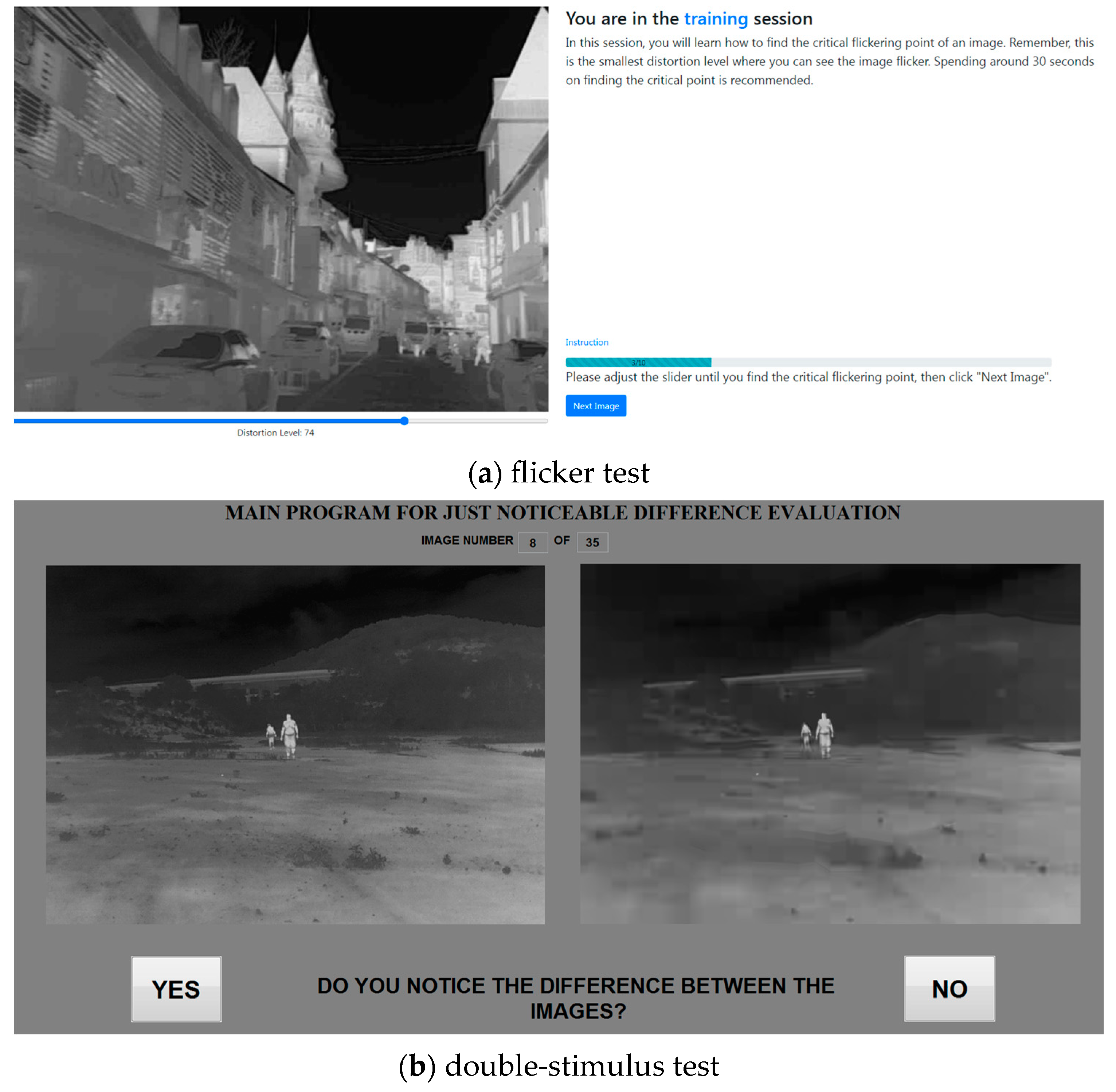
Figure 1.
Screenshots of the user interface for the picture-wise JND subjective tests: (a) flicker test and (b) double-stimulus test.
Figure 1.
Screenshots of the user interface for the picture-wise JND subjective tests: (a) flicker test and (b) double-stimulus test.
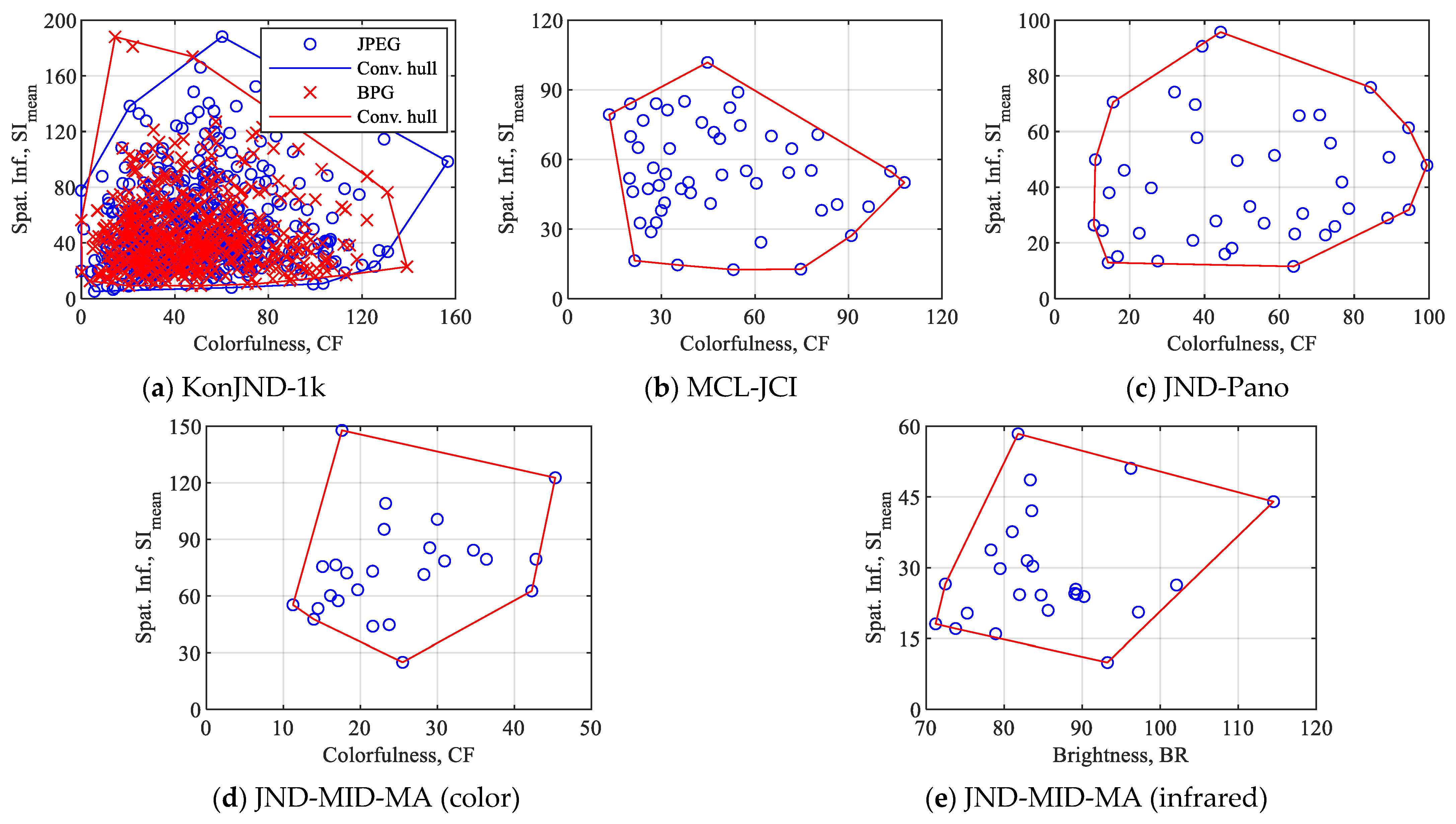
Figure 2.
Spatial information versus colorfulness and brightness and the corresponding convex hulls for the used databases: (a) KonJND-1k, (b) MCL-JCI, (c) JND-Pano, (d) JND-MID-MA (color), and (e) JND-MID-MA (infrared).
Figure 2.
Spatial information versus colorfulness and brightness and the corresponding convex hulls for the used databases: (a) KonJND-1k, (b) MCL-JCI, (c) JND-Pano, (d) JND-MID-MA (color), and (e) JND-MID-MA (infrared).
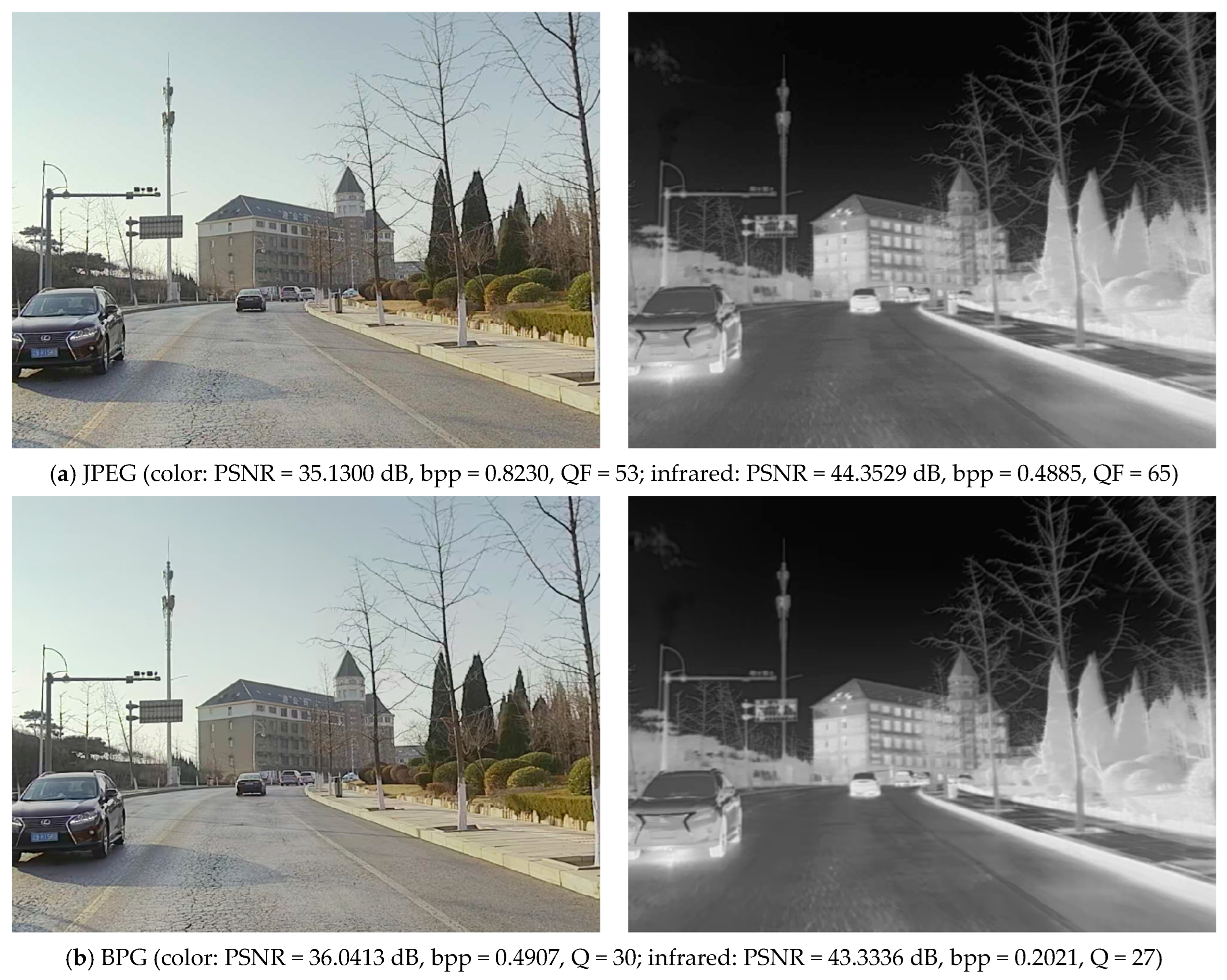
Figure 3.
Examples of color and infrared JND images from the JND-MID-MA database for (a) JPEG and (b) BPG (chroma format 4:2:2) compressions.
Figure 3.
Examples of color and infrared JND images from the JND-MID-MA database for (a) JPEG and (b) BPG (chroma format 4:2:2) compressions.
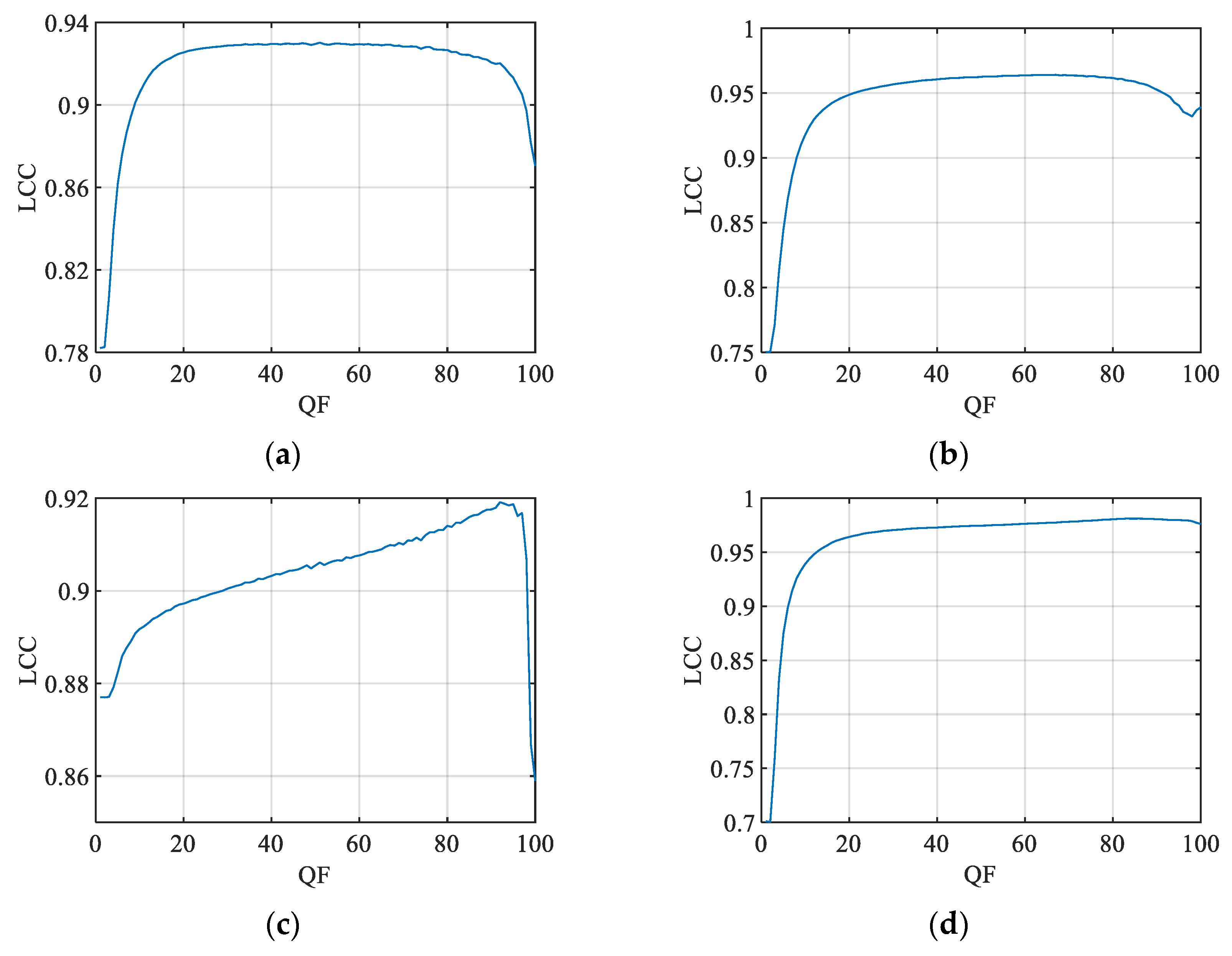
Figure 4.
LCC between the ground truth and predicted PSNR JND#1 values based on the CR calculated for different values of QF for the following: (a) KonJND-1k; (b) MCL-JCI; (c) JND-Pano; and (d) JND-MID-MA (25 color images) databases.
Figure 4.
LCC between the ground truth and predicted PSNR JND#1 values based on the CR calculated for different values of QF for the following: (a) KonJND-1k; (b) MCL-JCI; (c) JND-Pano; and (d) JND-MID-MA (25 color images) databases.
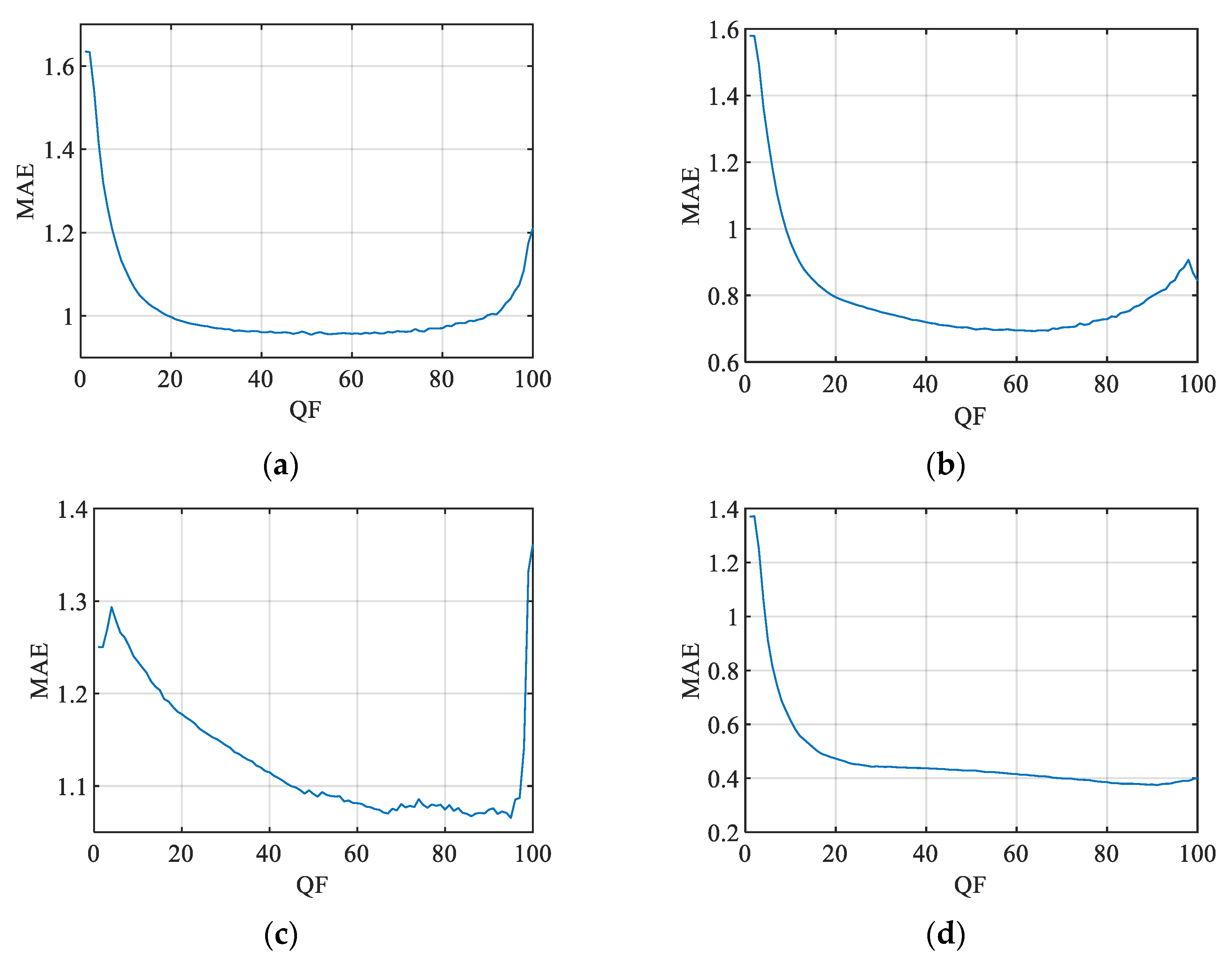
Figure 5.
MAE between the ground truth and PSNR JND#1 predicted values based on the CR calculated for different values of QF for the following: (a) KonJND-1k; (b) MCL-JCI; (c) JND-Pano; and (d) JND-MID-MA (25 color images) databases.
Figure 5.
MAE between the ground truth and PSNR JND#1 predicted values based on the CR calculated for different values of QF for the following: (a) KonJND-1k; (b) MCL-JCI; (c) JND-Pano; and (d) JND-MID-MA (25 color images) databases.
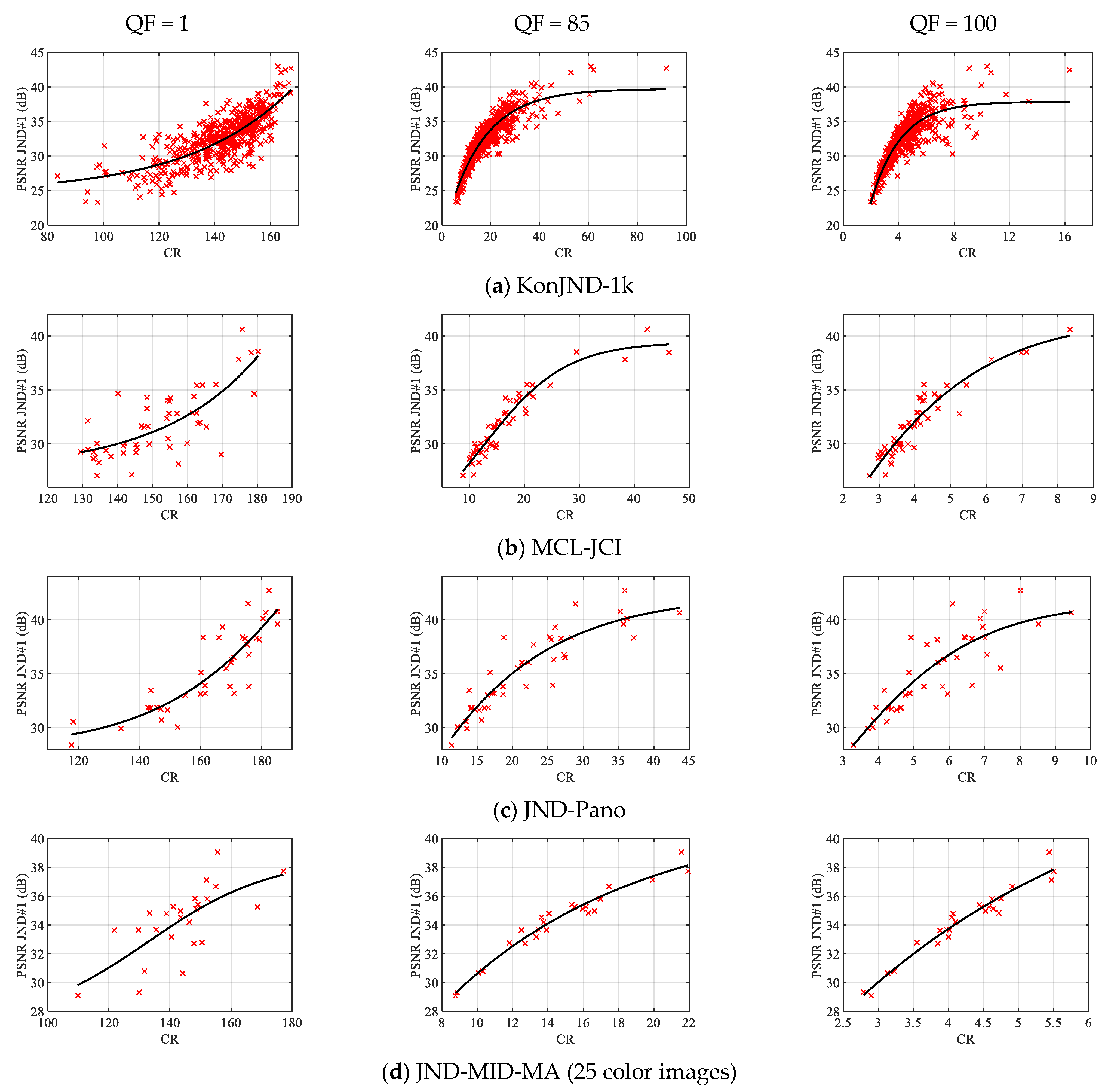
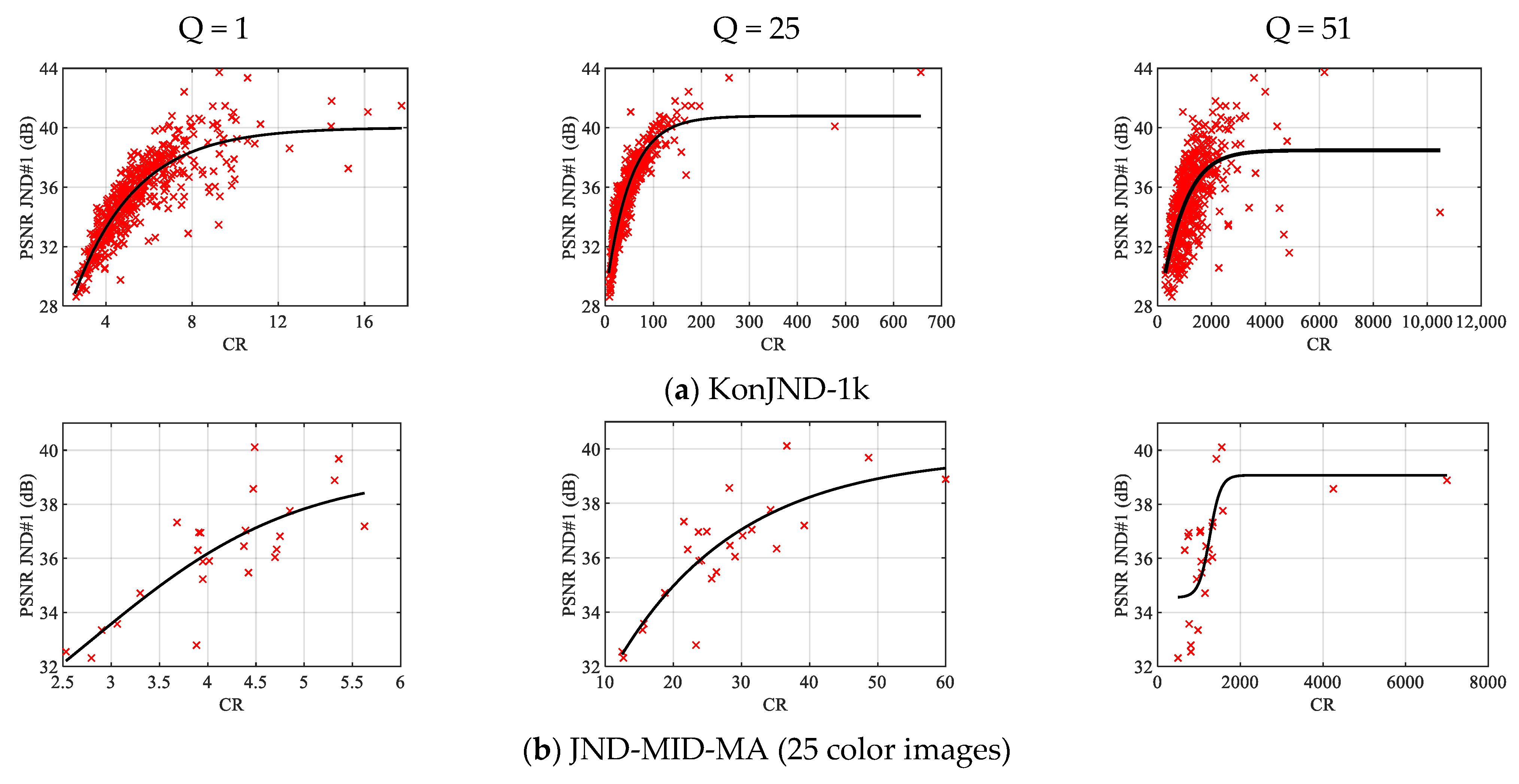
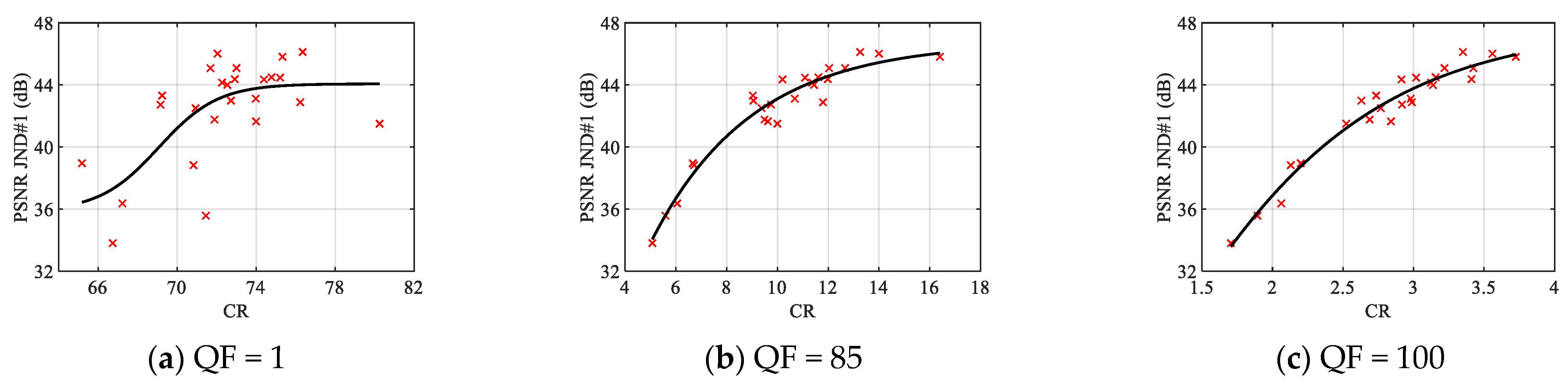
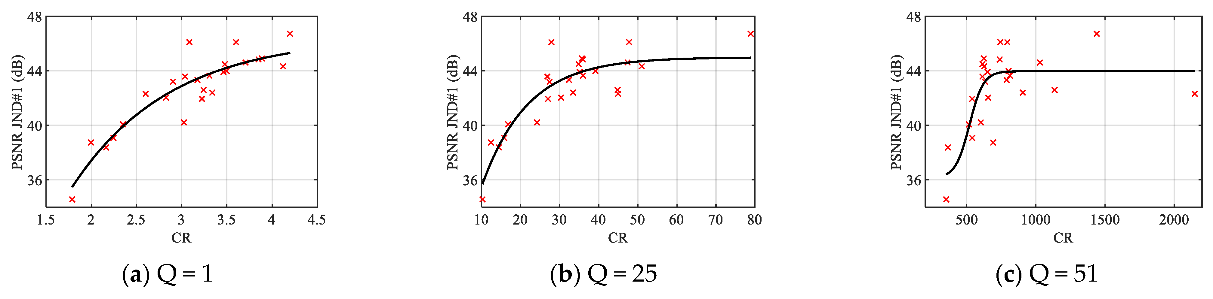
Figure 6.
CR vs. PSNR JND#1 scatter plots for three selected QF values and four databases.
Figure 6.
CR vs. PSNR JND#1 scatter plots for three selected QF values and four databases.
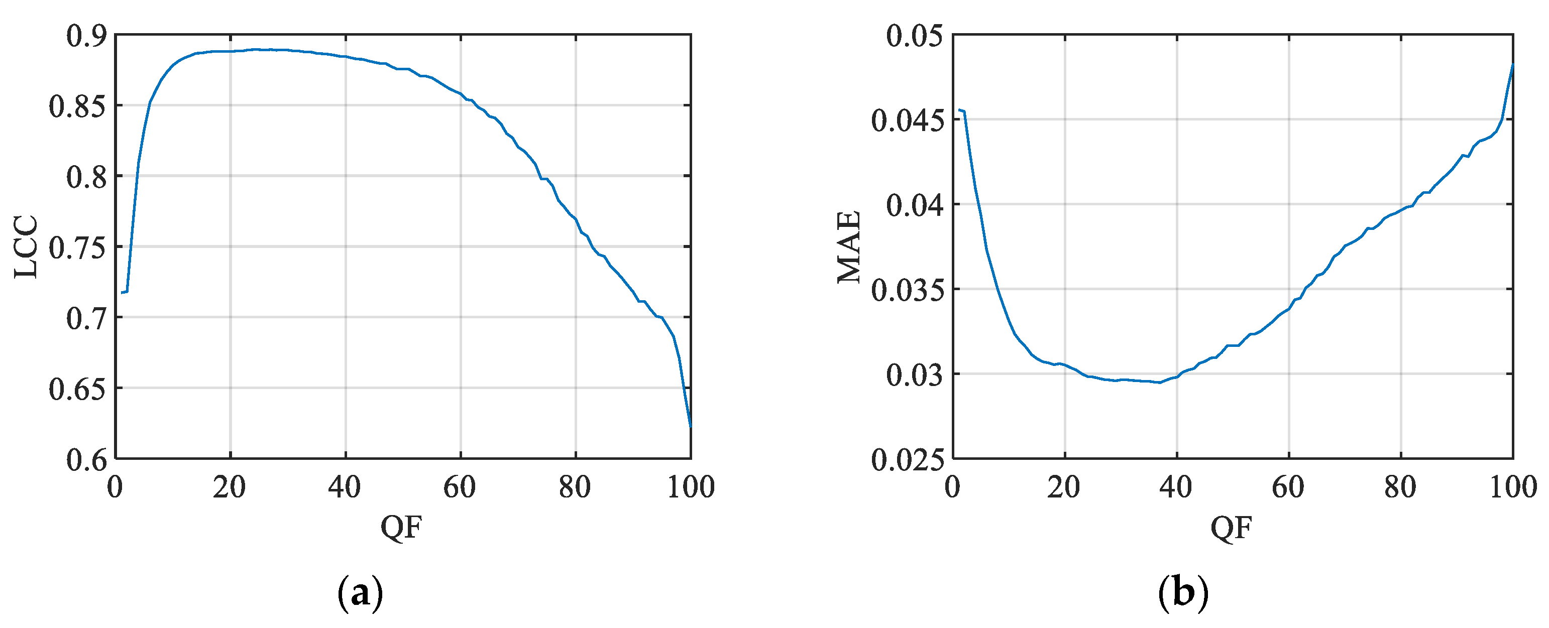
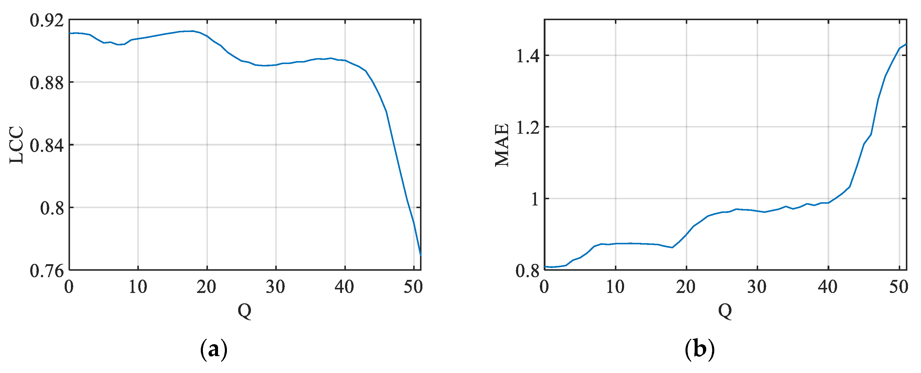
Figure 7.
LCC between the ground truth and predicted bpp JND#1 values based on the CR calculated for different values of QF for the following: (a) KonJND-1k; (b) MCL-JCI; (c) JND-Pano; and (d) JND-MID-MA (25 color images) databases.
Figure 7.
LCC between the ground truth and predicted bpp JND#1 values based on the CR calculated for different values of QF for the following: (a) KonJND-1k; (b) MCL-JCI; (c) JND-Pano; and (d) JND-MID-MA (25 color images) databases.
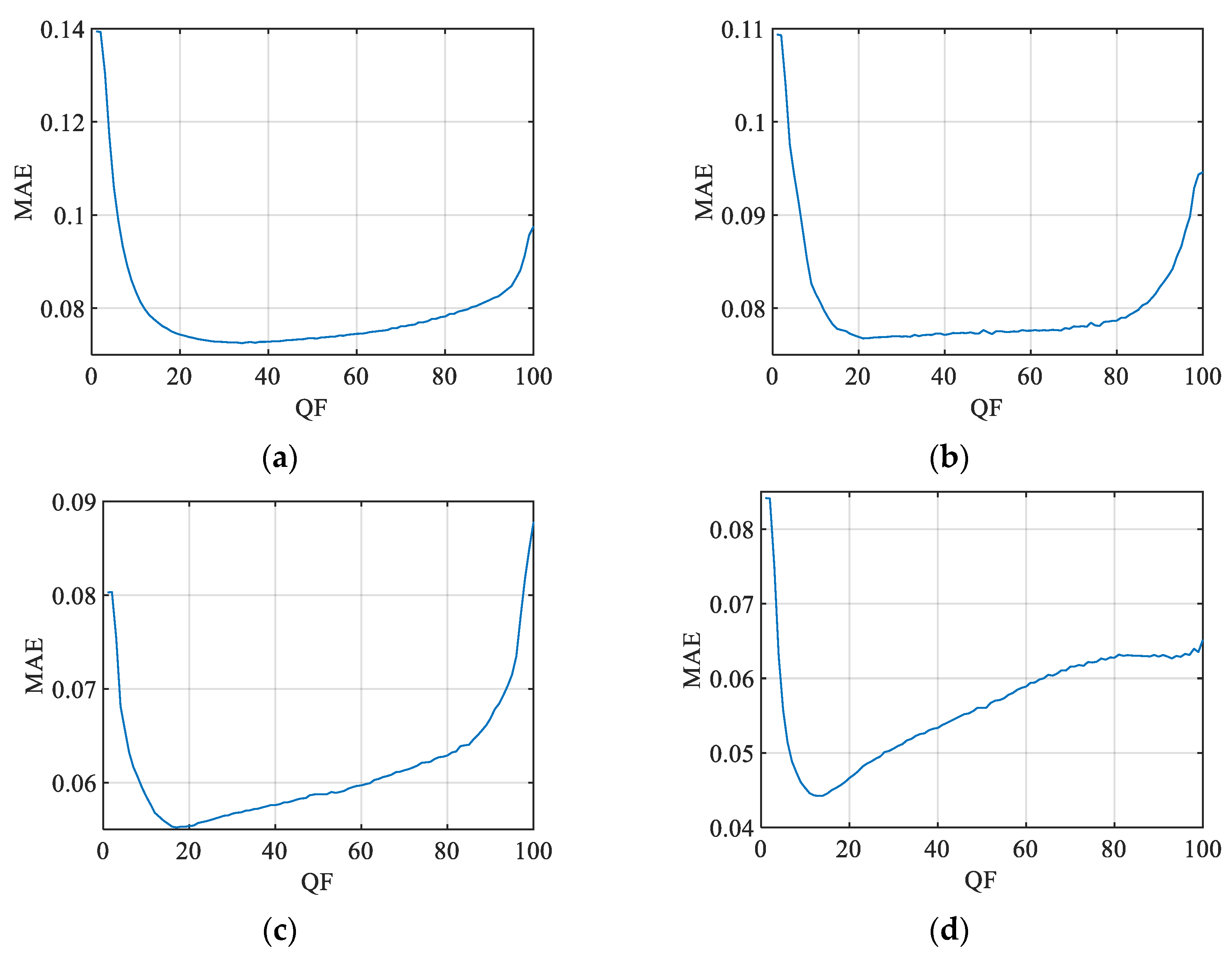
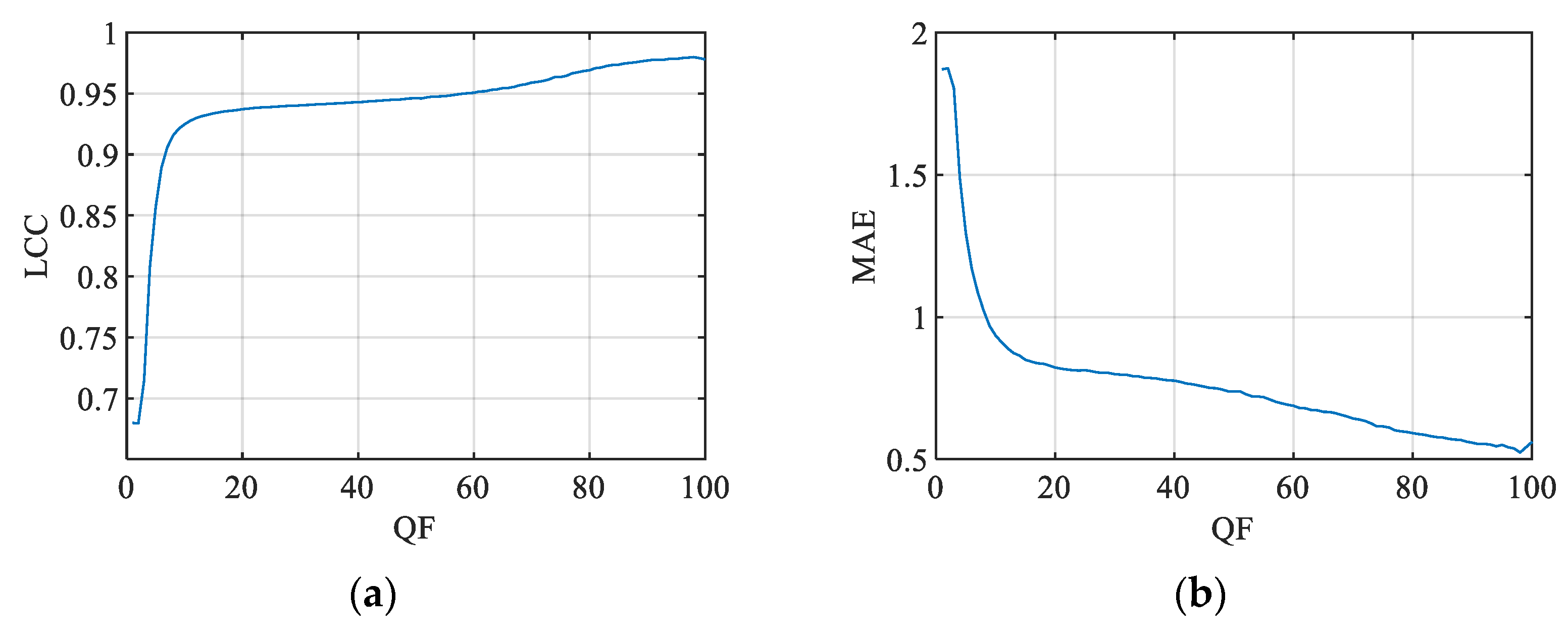
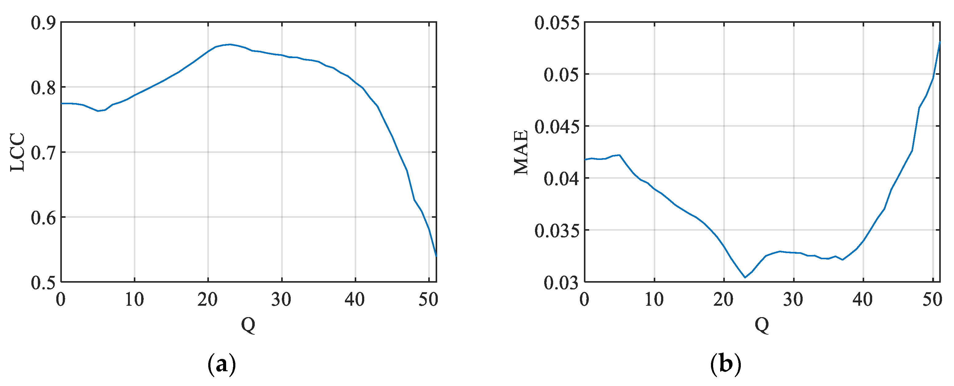
Figure 8.
MAE between the ground truth and bpp JND#1 predicted values based on the CR calculated for different values of QF for the following: (a) KonJND-1k; (b) MCL-JCI; (c) JND-Pano; and (d) JND-MID-MA (25 color images) databases.
Figure 8.
MAE between the ground truth and bpp JND#1 predicted values based on the CR calculated for different values of QF for the following: (a) KonJND-1k; (b) MCL-JCI; (c) JND-Pano; and (d) JND-MID-MA (25 color images) databases.
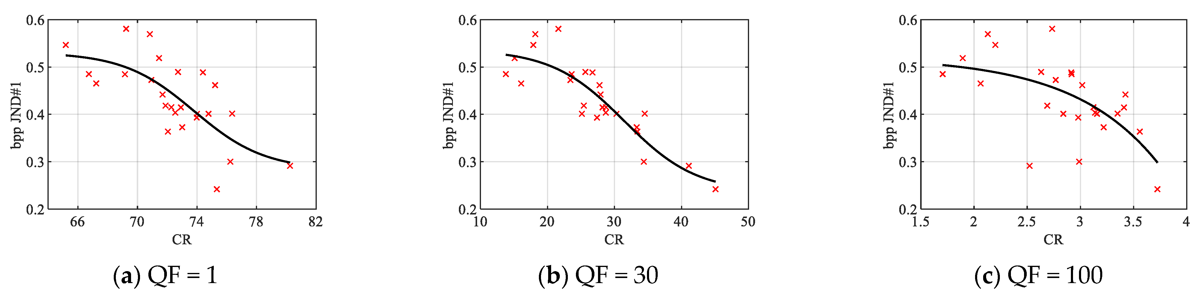
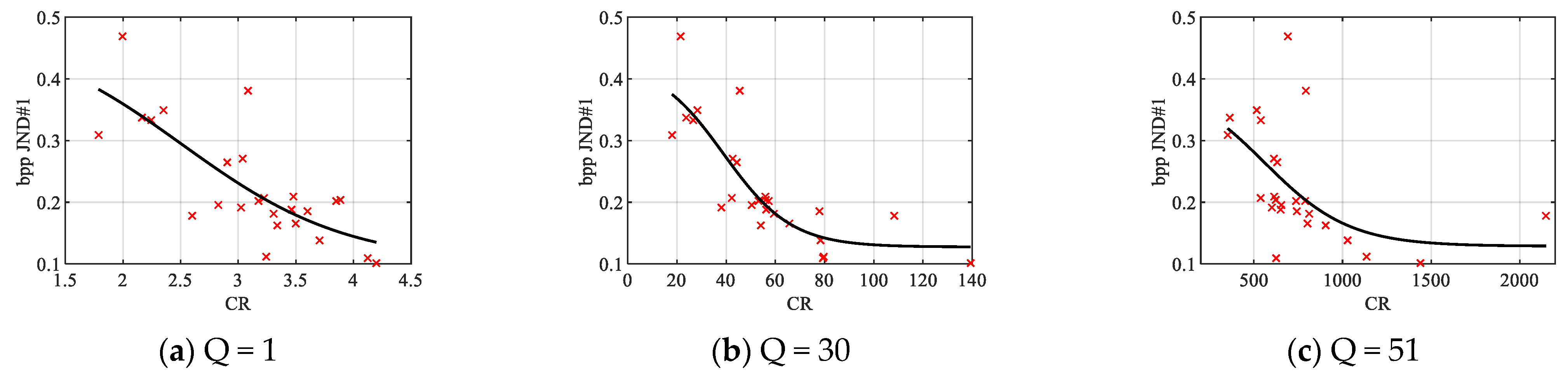
Figure 9.
CR vs. bpp JND#1 scatter plots for three selected QF values and four databases.
Figure 9.
CR vs. bpp JND#1 scatter plots for three selected QF values and four databases.
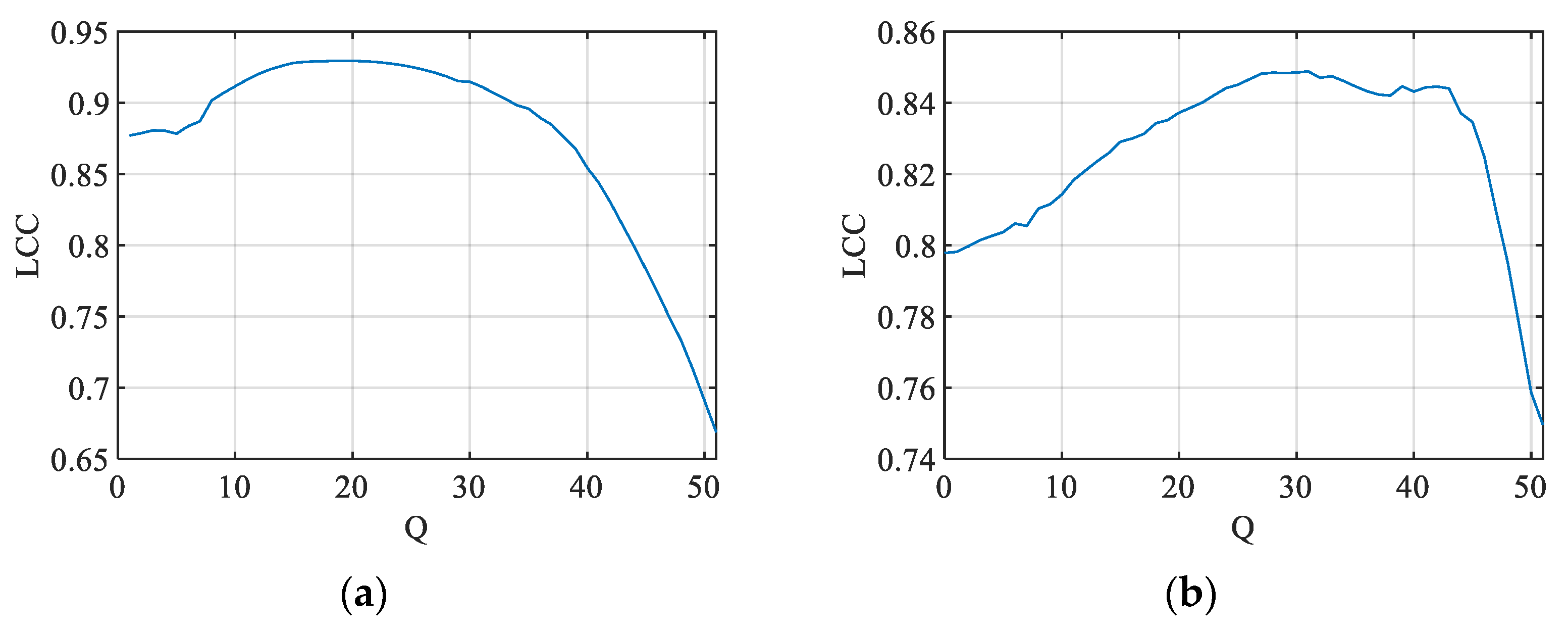
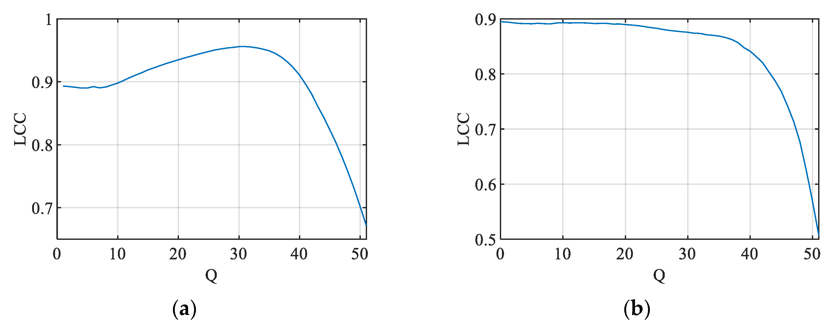
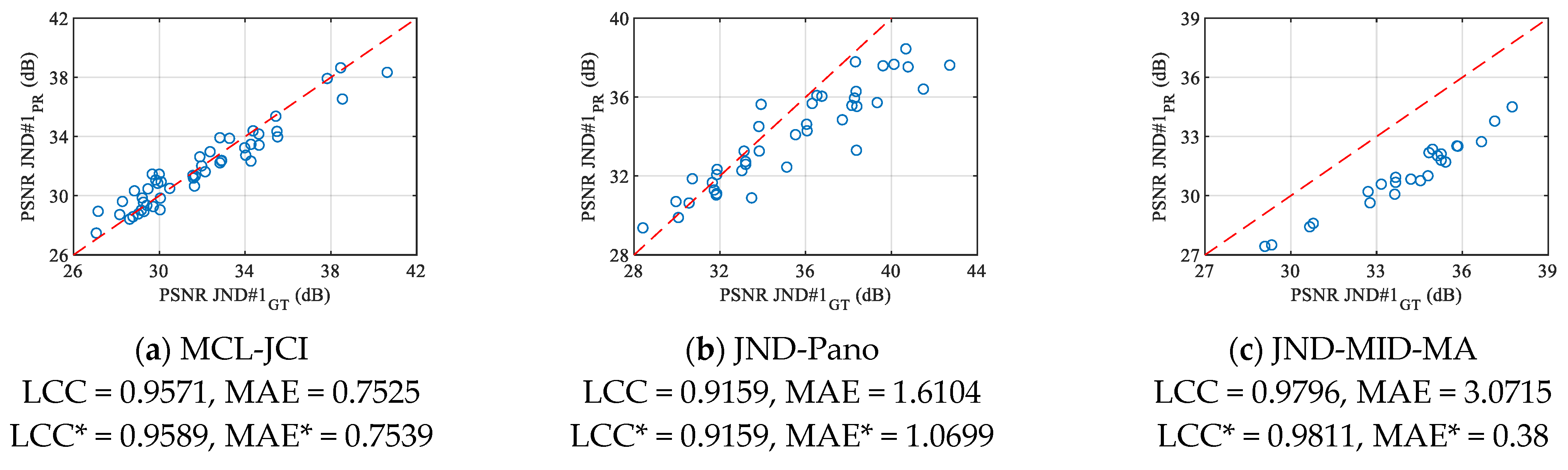
Figure 10.
LCC between the ground truth and predicted PSNR JND#1 values based on the CR calculated for different values of Q for (a) KonJND-1k and (b) JND-MID-MA (25 color images) databases.
Figure 10.
LCC between the ground truth and predicted PSNR JND#1 values based on the CR calculated for different values of Q for (a) KonJND-1k and (b) JND-MID-MA (25 color images) databases.
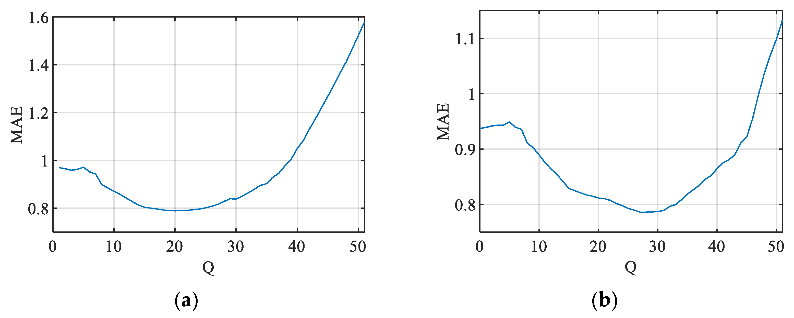
Figure 11.
MAE between the ground truth and predicted PSNR JND#1 values based on the CR calculated for different values of Q for (a) KonJND-1k and (b) JND-MID-MA (25 color images) databases.
Figure 11.
MAE between the ground truth and predicted PSNR JND#1 values based on the CR calculated for different values of Q for (a) KonJND-1k and (b) JND-MID-MA (25 color images) databases.
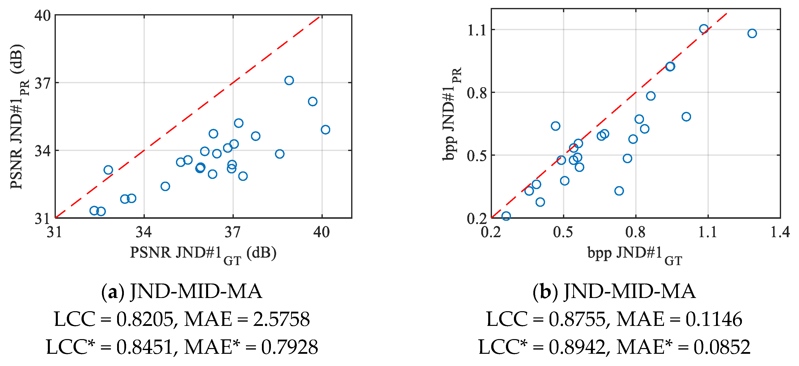
Figure 12.
CR vs. PSNR JND#1 scatter plots for three selected Q values and two databases.
Figure 12.
CR vs. PSNR JND#1 scatter plots for three selected Q values and two databases.
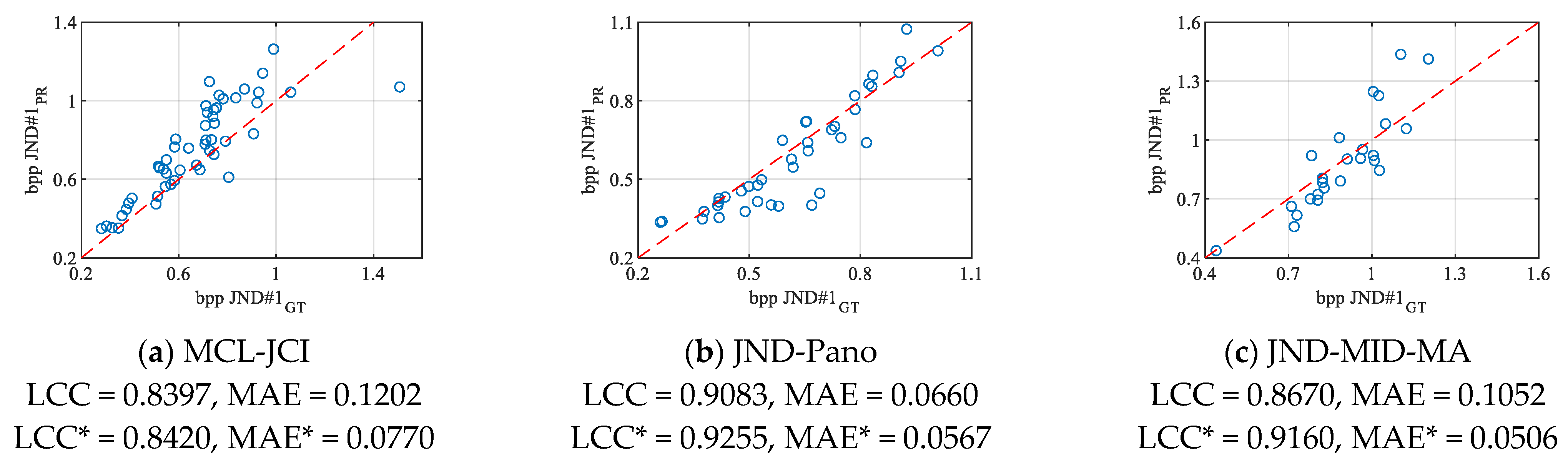
Figure 13.
LCC between the ground truth and predicted bpp JND#1 values based on the CR calculated for different values of Q for (a) KonJND-1k and (b) JND-MID-MA (25 color images) databases.
Figure 13.
LCC between the ground truth and predicted bpp JND#1 values based on the CR calculated for different values of Q for (a) KonJND-1k and (b) JND-MID-MA (25 color images) databases.
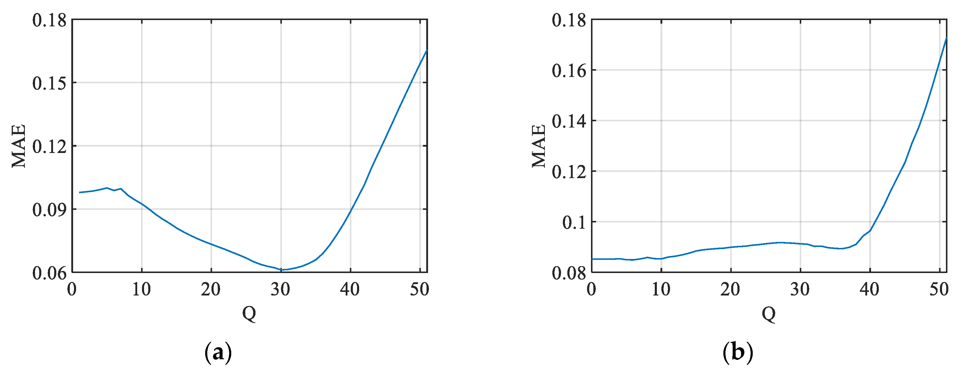
Figure 14.
MAE between the ground truth and predicted bpp JND#1 values based on the CR calculated for different values of Q for (a) KonJND-1k and (b) JND-MID-MA (25 color images) databases.
Figure 14.
MAE between the ground truth and predicted bpp JND#1 values based on the CR calculated for different values of Q for (a) KonJND-1k and (b) JND-MID-MA (25 color images) databases.
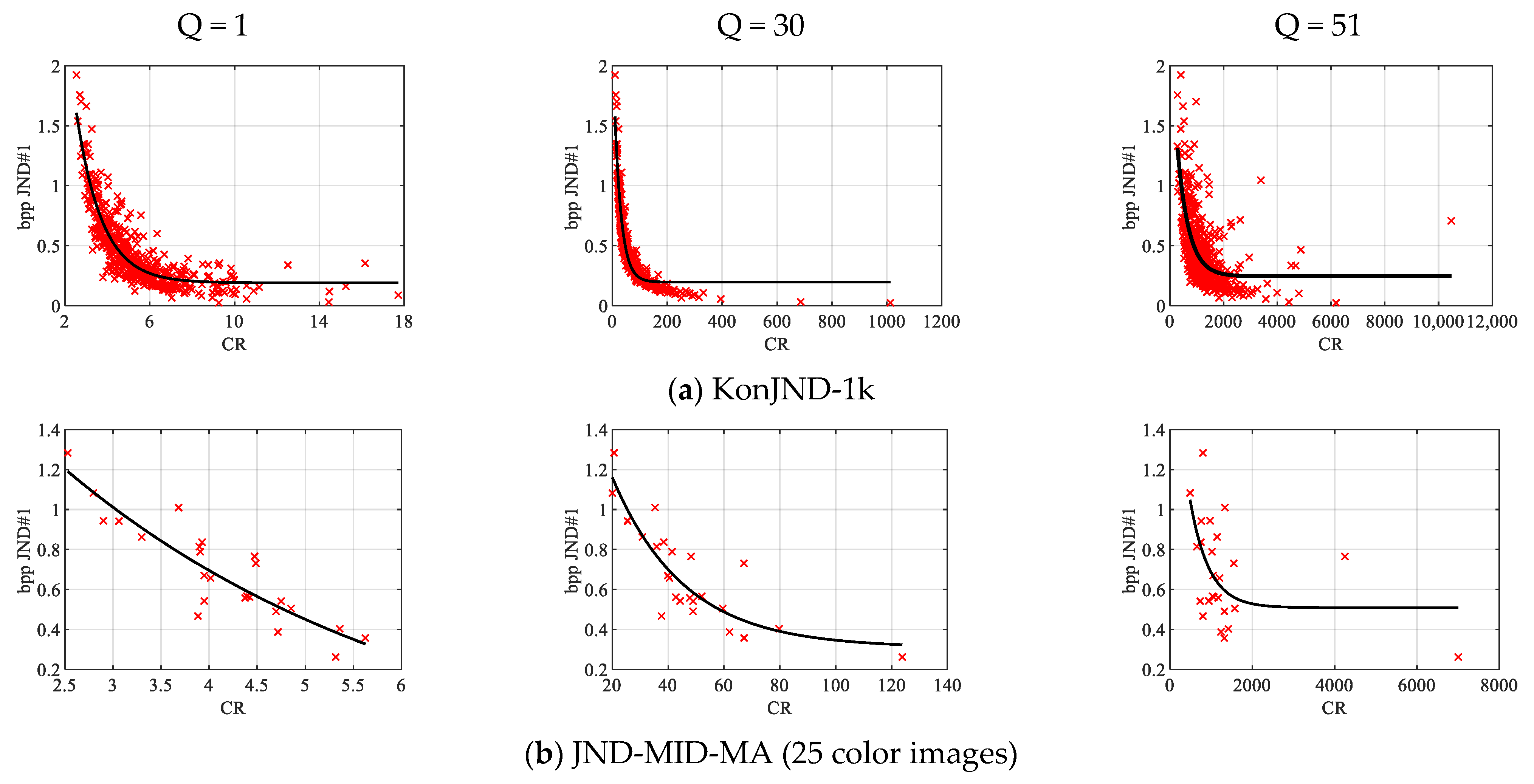
Figure 15.
CR vs. bpp JND#1 scatter plots for three selected Q values and two databases.
Figure 15.
CR vs. bpp JND#1 scatter plots for three selected Q values and two databases.
Figure 16.
(a) LCC and (b) MAE between the ground truth and PSNR JND#1 predicted values based on the CR calculated for different values of QF for JND-MID-MA database (25 infrared images).
Figure 16.
(a) LCC and (b) MAE between the ground truth and PSNR JND#1 predicted values based on the CR calculated for different values of QF for JND-MID-MA database (25 infrared images).
Figure 17.
(a) LCC and (b) MAE between the ground truth and bpp JND#1 predicted values based on the CR calculated for different values of QF for JND-MID-MA database (25 infrared images).
Figure 17.
(a) LCC and (b) MAE between the ground truth and bpp JND#1 predicted values based on the CR calculated for different values of QF for JND-MID-MA database (25 infrared images).
Figure 18.
CR vs. PSNR JND#1 scatter plots for three selected QF values for JND-MID-MA database (25 infrared images).
Figure 18.
CR vs. PSNR JND#1 scatter plots for three selected QF values for JND-MID-MA database (25 infrared images).
Figure 19.
CR vs. bpp JND#1 scatter plots for three selected QF values for JND-MID-MA database (25 infrared images).
Figure 19.
CR vs. bpp JND#1 scatter plots for three selected QF values for JND-MID-MA database (25 infrared images).
Figure 20.
(a) LCC and (b) MAE between the ground truth and PSNR JND#1 predicted values based on the CR calculated for different values of Q for JND-MID-MA database (25 infrared images).
Figure 20.
(a) LCC and (b) MAE between the ground truth and PSNR JND#1 predicted values based on the CR calculated for different values of Q for JND-MID-MA database (25 infrared images).
Figure 21.
(a) LCC and (b) MAE between the ground truth and bpp JND#1 predicted values based on the CR calculated for different values of Q for JND-MID-MA database (25 infrared images).
Figure 21.
(a) LCC and (b) MAE between the ground truth and bpp JND#1 predicted values based on the CR calculated for different values of Q for JND-MID-MA database (25 infrared images).
Figure 22.
CR vs. PSNR JND#1 scatter plots for three selected Q values for JND-MID-MA database (25 infrared images).
Figure 22.
CR vs. PSNR JND#1 scatter plots for three selected Q values for JND-MID-MA database (25 infrared images).
Figure 23.
CR vs. bpp JND#1 scatter plots for three selected Q values for JND-MID-MA database (25 infrared images).
Figure 23.
CR vs. bpp JND#1 scatter plots for three selected Q values for JND-MID-MA database (25 infrared images).
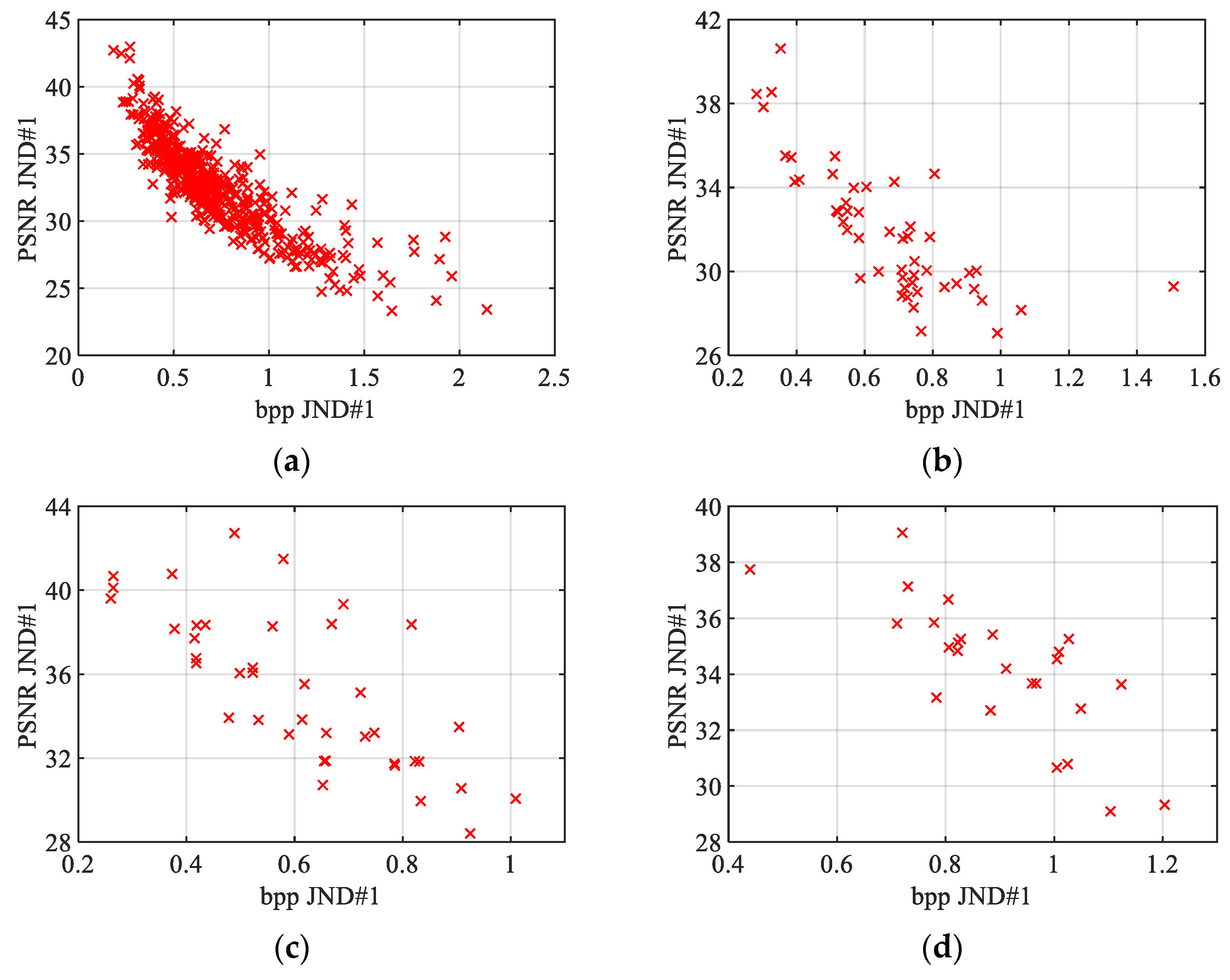
Figure 24.
Relationship between bpp JND#1 and PSNR JND#1 JPEG compressed color images for (a) KonJND-1k, (b) MCL-JCI, (c) JND-Pano, and (d) JND-MID-MA (25 color images) databases.
Figure 24.
Relationship between bpp JND#1 and PSNR JND#1 JPEG compressed color images for (a) KonJND-1k, (b) MCL-JCI, (c) JND-Pano, and (d) JND-MID-MA (25 color images) databases.
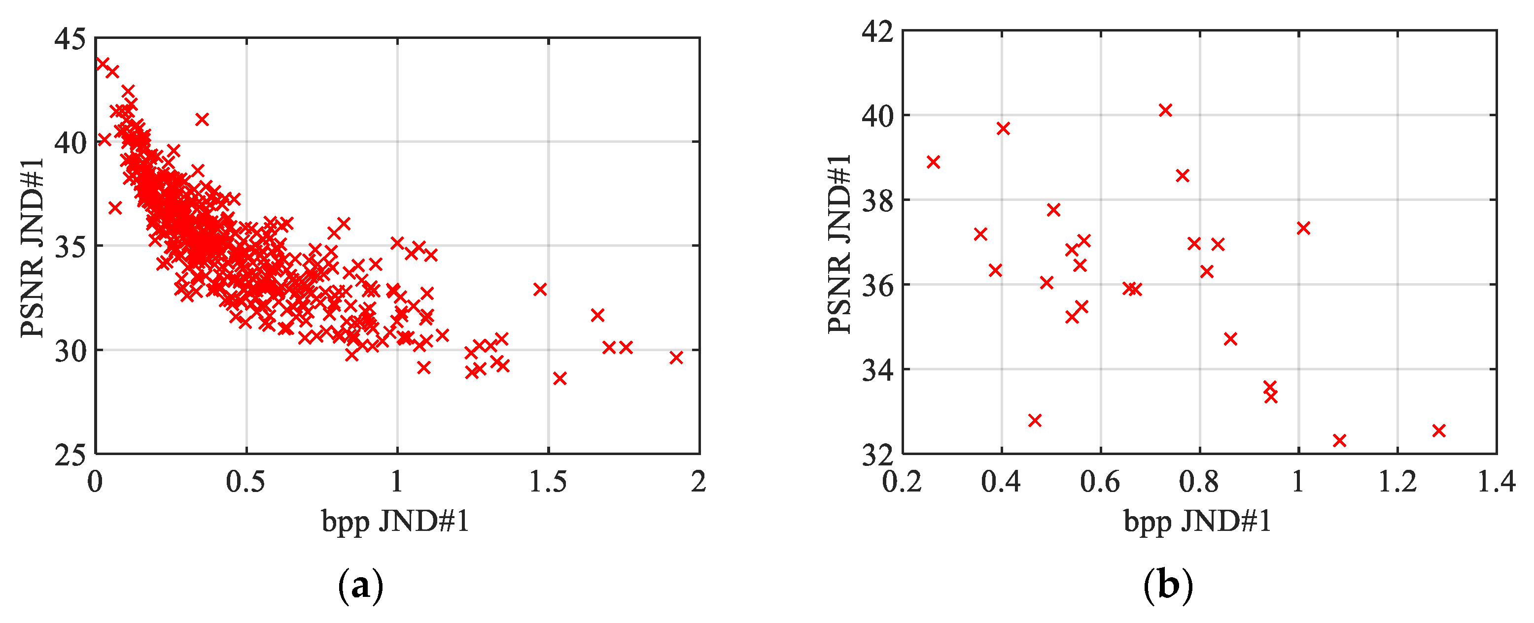
Figure 25.
Relationship between bpp JND#1 and PSNR JND#1 BPG compressed color images for (a) KonJND-1k and (b) JND-MID-MA (25 color images) databases.
Figure 25.
Relationship between bpp JND#1 and PSNR JND#1 BPG compressed color images for (a) KonJND-1k and (b) JND-MID-MA (25 color images) databases.
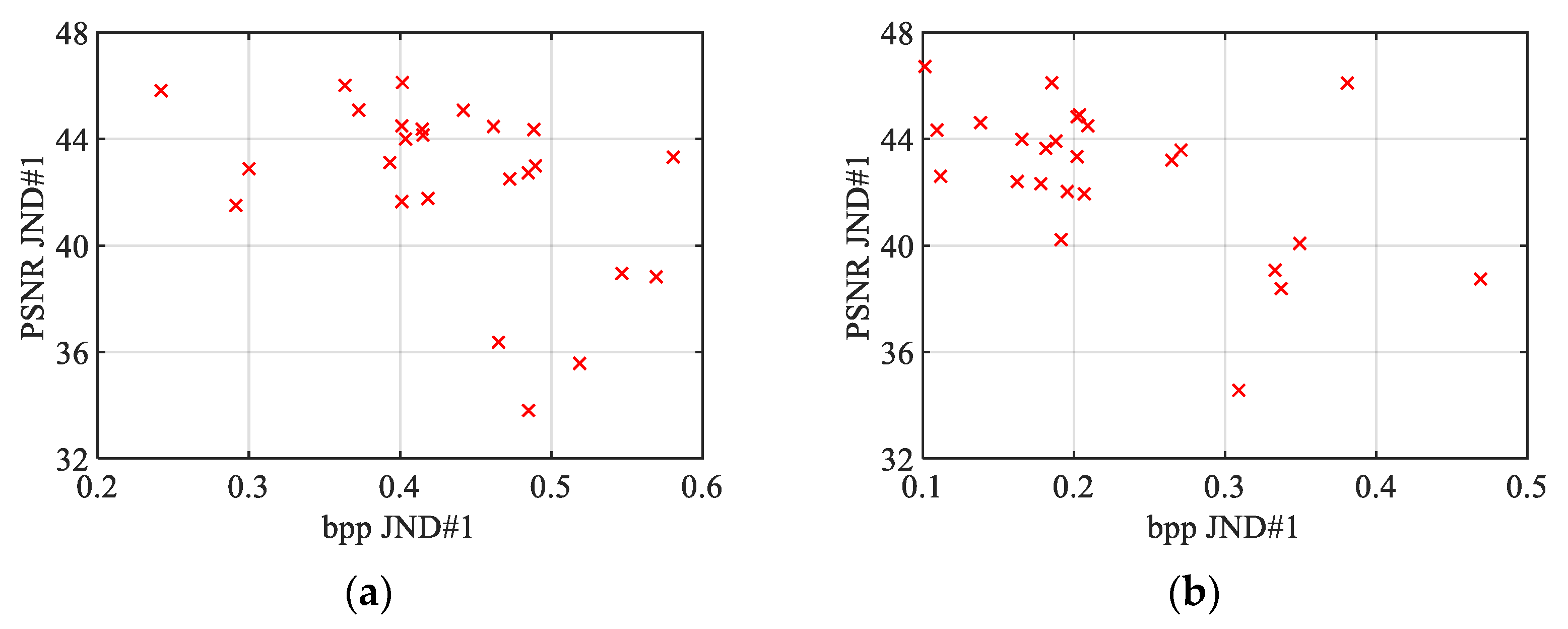
Figure 26.
Relationship between bpp JND#1 and PSNR JND#1 of infrared images JND-MID-MA database for (a) JPEG and (b) BPG compressions.
Figure 26.
Relationship between bpp JND#1 and PSNR JND#1 of infrared images JND-MID-MA database for (a) JPEG and (b) BPG compressions.
Figure 27.
Examples of JPEG compressed images corresponding to the first JND points obtained using the optimal CR to PSNR JND#1 mapping law valid for the KonJND-1k database.
Figure 27.
Examples of JPEG compressed images corresponding to the first JND points obtained using the optimal CR to PSNR JND#1 mapping law valid for the KonJND-1k database.
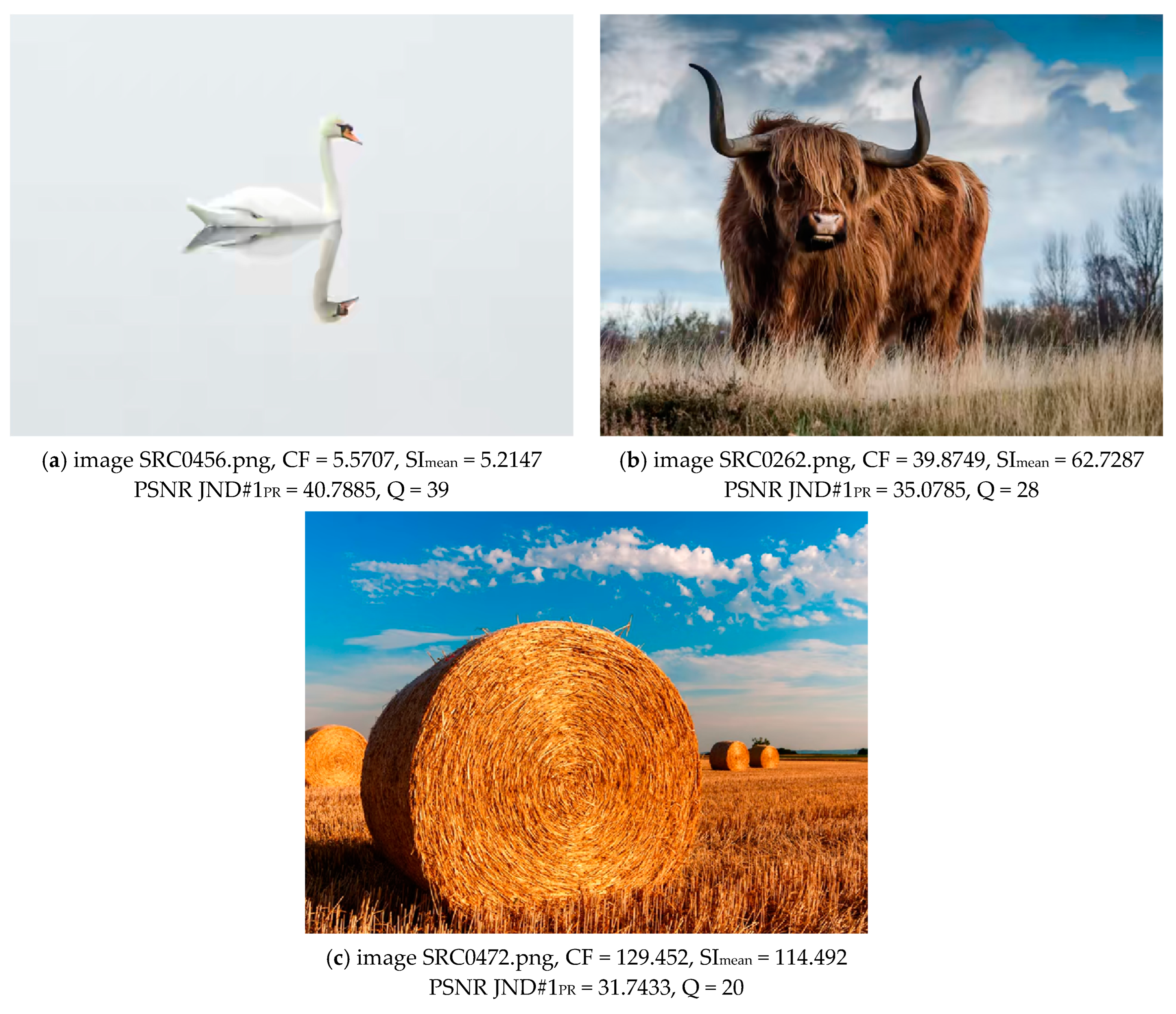
Figure 28.
Examples of BPG compressed images corresponding to the first JND points obtained using the optimal CR to PSNR JND#1 mapping law valid for the KonJND-1k database.
Figure 28.
Examples of BPG compressed images corresponding to the first JND points obtained using the optimal CR to PSNR JND#1 mapping law valid for the KonJND-1k database.
Figure 29.
Relationships between KonJND-1k guided PSNR predictions and ground truth PSNR JND#1 values of JPEG compressed images for (a) MCL-JCI, (b) JND-Pano, and (c) JND-MID-MA color databases.
Figure 29.
Relationships between KonJND-1k guided PSNR predictions and ground truth PSNR JND#1 values of JPEG compressed images for (a) MCL-JCI, (b) JND-Pano, and (c) JND-MID-MA color databases.
Figure 30.
Relationships between KonJND-1k guided bpp predictions and ground truth bpp JND#1 values of JPEG compressed images for (a) MCL-JCI, (b) JND-Pano, and (c) JND-MID-MA color databases.
Figure 30.
Relationships between KonJND-1k guided bpp predictions and ground truth bpp JND#1 values of JPEG compressed images for (a) MCL-JCI, (b) JND-Pano, and (c) JND-MID-MA color databases.
Figure 31.
Relationships between KonJND-1k guided PSNR/bpp predictions and ground truth PSNR/bpp JND#1 values of BPG compressed images of JND-MID-MA color database.
Figure 31.
Relationships between KonJND-1k guided PSNR/bpp predictions and ground truth PSNR/bpp JND#1 values of BPG compressed images of JND-MID-MA color database.
Table 1.
Basic characteristics of the used JND databases.
Table 1.
Basic characteristics of the used JND databases.
| Database | Publication Year | Image Size (In Pixels) | Number of Reference Images | Distortion Type | Distortion Levels Per Reference | Number of Test Stimuli | Number of Observers | Subjective Test | Test
Environment |
|---|
| MCL-JCI [36] | 2016 | 1920 × 1080 | 50 | JPEG | 100 | 5000 | 30 | side by side + binary search | lab |
| JND-Pano [37] | 2018 | 5000 × 2500 | 40 | JPEG | 100 | 4000 | 42 (at least 25 per image) | side by side + binary search | lab |
| KonJND-1k [38] | 2022 | 640 × 480 | 504 | JPEG | 100 | 50,400 | 503 (an average of 42 per image) | flicker test | crowdsourcing |
| 504 | BPG | 51 | 25,704 |
| JND-MID-MA [39] | 2024 | variable | 105 (35 color, 35 grayscale, and 35 infrared) | JPEG | 100 | 3500 × 3 | 26 (color), 19 (grayscale) and 22 (infrared) | side by side + binary search | lab |
| BPG | 52 | 1820 × 3 | 29 (color), 27 (grayscale), and 27 (infrared) |
Table 2.
Quantitative indicators of the degree of agreement between ground truth and PSNR JND#1 predictions obtained using CR (calculated for three quality factors), SImean, contrast, homogeneity, and edge density for four databases.
Table 2.
Quantitative indicators of the degree of agreement between ground truth and PSNR JND#1 predictions obtained using CR (calculated for three quality factors), SImean, contrast, homogeneity, and edge density for four databases.
| | | LCC | SROCC | MAE | RMSE | LCC | SROCC | MAE | RMSE |
|---|
| Database | KonJND-1k | MCL-JCI |
| CR | QF = 1 | 0.7822 | 0.7504 | 1.6350 | 2.0652 | 0.7504 | 0.6648 | 1.5791 | 2.0265 |
| QF = 85 | 0.9243 | 0.9164 | 0.9826 | 1.2650 | 0.9589 | 0.9455 | 0.7539 | 0.8694 |
| QF = 100 | 0.8705 | 0.8518 | 1.2108 | 1.6312 | 0.9392 | 0.9349 | 0.8442 | 1.0524 |
| SImean | | 0.9110 | 0.9021 | 1.0789 | 1.3668 | 0.9398 | 0.9090 | 0.8528 | 1.0476 |
| contrast | | 0.8728 | 0.8750 | 1.2425 | 1.6176 | 0.8805 | 0.8250 | 1.1540 | 1.4534 |
| homogeneity | | 0.7465 | 0.7073 | 1.7224 | 2.2055 | 0.7746 | 0.7055 | 1.6140 | 1.9391 |
| edge density | | 0.7922 | 0.7851 | 1.5670 | 2.0228 | 0.8416 | 0.7387 | 1.3004 | 1.6561 |
| Database | JND-Pano | JND-MID-MA (25 Color Images) |
| CR | QF = 1 | 0.8770 | 0.8514 | 1.2504 | 1.7408 | 0.7010 | 0.7213 | 1.3702 | 1.7015 |
| QF = 85 | 0.9159 | 0.9221 | 1.0699 | 1.4541 | 0.9811 | 0.9662 | 0.3800 | 0.4617 |
| QF = 100 | 0.8590 | 0.8552 | 1.3613 | 1.8551 | 0.9762 | 0.9592 | 0.4018 | 0.5174 |
| SImean | | 0.9099 | 0.9205 | 1.1225 | 1.5032 | 0.9440 | 0.9446 | 0.6264 | 0.7874 |
| contrast | | 0.9515 | 0.9467 | 0.8656 | 1.1152 | 0.8392 | 0.8331 | 1.0447 | 1.2975 |
| homogeneity | | 0.7592 | 0.7452 | 1.8998 | 2.3581 | 0.9234 | 0.8885 | 0.7263 | 0.9156 |
| edge density | | 0.6420 | 0.6516 | 2.1834 | 2.7779 | 0.7787 | 0.6638 | 1.0672 | 1.4968 |
Table 3.
Quantitative indicators of the degree of agreement between ground truth and bpp JND#1 predictions obtained using CR (calculated for three quality factors), SImean, contrast, homogeneity, and edge density for four databases.
Table 3.
Quantitative indicators of the degree of agreement between ground truth and bpp JND#1 predictions obtained using CR (calculated for three quality factors), SImean, contrast, homogeneity, and edge density for four databases.
| | | LCC | SROCC | MAE | RMSE | LCC | SROCC | MAE | RMSE |
| Database | KonJND-1k | MCL-JCI |
| CR | QF = 1 | 0.7871 | 0.7926 | 0.1394 | 0.1913 | 0.7258 | 0.7551 | 0.1094 | 0.1510 |
| QF = 30 | 0.9347 | 0.9535 | 0.0727 | 0.1102 | 0.8420 | 0.8836 | 0.0770 | 0.1184 |
| QF = 100 | 0.9023 | 0.8832 | 0.0975 | 0.1337 | 0.7925 | 0.8306 | 0.0946 | 0.1338 |
| SImean | | 0.9051 | 0.9202 | 0.0890 | 0.1318 | 0.8399 | 0.9095 | 0.0770 | 0.1191 |
| contrast | | 0.8311 | 0.8229 | 0.1233 | 0.1724 | 0.8507 | 0.8971 | 0.0803 | 0.1153 |
| homogeneity | | 0.7954 | 0.7688 | 0.1367 | 0.1879 | 0.5573 | 0.6002 | 0.1268 | 0.1822 |
| edge density | | 0.8061 | 0.8137 | 0.1307 | 0.1835 | 0.6591 | 0.6319 | 0.1068 | 0.1650 |
| Database | JND-Pano | JND-MID-MA (25 Color Images) |
| CR | QF = 1 | 0.8547 | 0.8501 | 0.0803 | 0.0994 | 0.7737 | 0.6917 | 0.0842 | 0.1023 |
| QF = 30 | 0.9255 | 0.9034 | 0.0567 | 0.0725 | 0.9160 | 0.8585 | 0.0506 | 0.0648 |
| QF = 100 | 0.8191 | 0.7891 | 0.0878 | 0.1098 | 0.8508 | 0.8200 | 0.0652 | 0.0849 |
| SImean | | 0.9188 | 0.8991 | 0.0598 | 0.0756 | 0.9222 | 0.8585 | 0.0488 | 0.0624 |
| contrast | | 0.8458 | 0.8368 | 0.0804 | 0.1021 | 0.8527 | 0.7531 | 0.0655 | 0.0844 |
| homogeneity | | 0.7489 | 0.7473 | 0.1042 | 0.1269 | 0.6388 | 0.6354 | 0.0851 | 0.1242 |
| edge density | | 0.7308 | 0.6795 | 0.1037 | 0.1307 | 0.4938 | 0.5400 | 0.1024 | 0.1404 |
Table 4.
Quantitative indicators of the degree of agreement between ground truth and PSNR JND#1 predictions obtained using CR (calculated for three parameter Q values), SImean, contrast, homogeneity, and edge density for two databases.
Table 4.
Quantitative indicators of the degree of agreement between ground truth and PSNR JND#1 predictions obtained using CR (calculated for three parameter Q values), SImean, contrast, homogeneity, and edge density for two databases.
| | | LCC | SROCC | MAE | RMSE | LCC | SROCC | MAE | RMSE |
|---|
| Database | KonJND-1k | JND-MID-MA (25 Color Images) |
|---|
| CR | Q = 1 | 0.8771 | 0.8793 | 0.9700 | 1.2931 | 0.7981 | 0.7292 | 0.9388 | 1.2421 |
| Q = 25 | 0.9253 | 0.9265 | 0.8018 | 1.0210 | 0.8451 | 0.7723 | 0.7928 | 1.1021 |
| Q = 51 | 0.6687 | 0.6516 | 1.5781 | 2.0017 | 0.7496 | 0.6954 | 1.1328 | 1.3647 |
| SImean | | 0.8655 | 0.8599 | 1.0565 | 1.3484 | 0.8388 | 0.7892 | 0.9013 | 1.1226 |
| contrast | | 0.7406 | 0.7415 | 1.4123 | 1.8090 | 0.8126 | 0.7731 | 0.9791 | 1.2017 |
| homogeneity | | 0.7879 | 0.7834 | 1.2817 | 1.6580 | 0.7451 | 0.6485 | 0.9462 | 1.3750 |
| edge density | | 0.8242 | 0.8324 | 1.2098 | 1.5273 | 0.6091 | 0.5062 | 1.1631 | 1.6351 |
Table 5.
Quantitative indicators of the degree of agreement between ground truth and bpp JND#1 predictions obtained using CR (calculated for three parameter Q values), SImean, contrast, homogeneity, and edge density for two databases.
Table 5.
Quantitative indicators of the degree of agreement between ground truth and bpp JND#1 predictions obtained using CR (calculated for three parameter Q values), SImean, contrast, homogeneity, and edge density for two databases.
| | | LCC | SROCC | MAE | RMSE | LCC | SROCC | MAE | RMSE |
|---|
| Database | KonJND-1k | JND-MID-MA (25 Color Images) |
|---|
| CR | Q = 1 | 0.8933 | 0.8661 | 0.0978 | 0.1342 | 0.8942 | 0.8523 | 0.0852 | 0.1098 |
| Q = 30 | 0.9558 | 0.9722 | 0.0611 | 0.0877 | 0.8756 | 0.8385 | 0.0912 | 0.1185 |
| Q = 51 | 0.6717 | 0.6594 | 0.1655 | 0.2212 | 0.5065 | 0.4531 | 0.1729 | 0.2115 |
| SImean | | 0.9061 | 0.9043 | 0.0885 | 0.1263 | 0.8336 | 0.7762 | 0.1029 | 0.1355 |
| contrast | | 0.8231 | 0.8211 | 0.1226 | 0.1695 | 0.6530 | 0.5962 | 0.1491 | 0.1857 |
| homogeneity | | 0.7906 | 0.7697 | 0.1347 | 0.1828 | 0.8294 | 0.8023 | 0.1093 | 0.1370 |
| edge density | | 0.7970 | 0.8333 | 0.1271 | 0.1804 | 0.7493 | 0.6608 | 0.1146 | 0.1624 |
Table 6.
Quantitative indicators of the degree of agreement between ground truth and PSNR JND#1 predictions obtained using CR (calculated for three QF values), SImean, contrast, homogeneity, and edge density for JND-MID-MA database.
Table 6.
Quantitative indicators of the degree of agreement between ground truth and PSNR JND#1 predictions obtained using CR (calculated for three QF values), SImean, contrast, homogeneity, and edge density for JND-MID-MA database.
| | LCC | SROCC | MAE | RMSE |
|---|
| CR | QF = 1 | 0.6798 | 0.5323 | 1.8707 | 2.3667 |
| QF = 85 | 0.9736 | 0.9015 | 0.5766 | 0.7363 |
| QF = 100 | 0.9780 | 0.9300 | 0.5610 | 0.6726 |
| SImean | | 0.9310 | 0.6992 | 0.8909 | 1.1781 |
| contrast | | 0.9126 | 0.6154 | 1.0479 | 1.3193 |
| homogeneity | | 0.9678 | 0.8854 | 0.6692 | 0.8122 |
| edge density | | 0.9186 | 0.7223 | 1.1100 | 1.2755 |
Table 7.
Quantitative indicators of the degree of agreement between ground truth and bpp JND#1 predictions obtained using CR (calculated for three QF values), SImean, contrast, homogeneity, and edge density for JND-MID-MA database.
Table 7.
Quantitative indicators of the degree of agreement between ground truth and bpp JND#1 predictions obtained using CR (calculated for three QF values), SImean, contrast, homogeneity, and edge density for JND-MID-MA database.
| | LCC | SROCC | MAE | RMSE |
|---|
| CR | QF = 1 | 0.7173 | 0.7146 | 0.0456 | 0.0566 |
| QF = 30 | 0.8888 | 0.8408 | 0.0296 | 0.0372 |
| QF = 100 | 0.6222 | 0.6331 | 0.0483 | 0.0636 |
| SImean | | 0.9046 | 0.8885 | 0.0277 | 0.0346 |
| contrast | | 0.8562 | 0.8046 | 0.0335 | 0.0420 |
| homogeneity | | 0.6876 | 0.6823 | 0.0444 | 0.0590 |
| edge density | | 0.5638 | 0.6077 | 0.0501 | 0.0671 |
Table 8.
Quantitative indicators of the degree of agreement between ground truth and PSNR JND#1 predictions obtained using CR (calculated for three parameter Q values), SImean, contrast, homogeneity, and edge density for JND-MID-MA database.
Table 8.
Quantitative indicators of the degree of agreement between ground truth and PSNR JND#1 predictions obtained using CR (calculated for three parameter Q values), SImean, contrast, homogeneity, and edge density for JND-MID-MA database.
| | LCC | SROCC | MAE | RMSE |
|---|
| CR | Q = 1 | 0.9113 | 0.8692 | 0.8079 | 1.1404 |
| Q = 25 | 0.8935 | 0.7669 | 0.9613 | 1.2439 |
| Q = 51 | 0.7690 | 0.5092 | 1.4317 | 1.7705 |
| SImean | | 0.9062 | 0.7038 | 0.9053 | 1.1709 |
| contrast | | 0.9073 | 0.6715 | 0.9167 | 1.1646 |
| homogeneity | | 0.9056 | 0.8746 | 0.8770 | 1.1748 |
| edge density | | 0.7517 | 0.7108 | 1.3542 | 1.8266 |
Table 9.
Quantitative indicators of the degree of agreement between ground truth and bpp JND#1 predictions obtained using CR (calculated for three parameter Q values), SImean, contrast, homogeneity, and edge density for JND-MID-MA database.
Table 9.
Quantitative indicators of the degree of agreement between ground truth and bpp JND#1 predictions obtained using CR (calculated for three parameter Q values), SImean, contrast, homogeneity, and edge density for JND-MID-MA database.
| | LCC | SROCC | MAE | RMSE |
|---|
| CR | Q = 1 | 0.7747 | 0.6854 | 0.0419 | 0.0568 |
| Q = 30 | 0.8490 | 0.8623 | 0.0328 | 0.0475 |
| Q = 51 | 0.5390 | 0.6654 | 0.0531 | 0.0757 |
| SImean | | 0.8029 | 0.8462 | 0.0359 | 0.0536 |
| SFmean | | 0.8150 | 0.8508 | 0.0345 | 0.0521 |
| contrast | | 0.7196 | 0.7631 | 0.0412 | 0.0624 |
| homogeneity | | 0.8053 | 0.6792 | 0.0407 | 0.0533 |
| edge density | | 0.8181 | 0.5623 | 0.0417 | 0.0517 |
Table 10.
Optimum values of the logistic function coefficients (β1–β4) for the prediction of the JND#1 position obtained for the KonJND-1k database.
Table 10.
Optimum values of the logistic function coefficients (β1–β4) for the prediction of the JND#1 position obtained for the KonJND-1k database.
| | β1 | β2 | β3 | β4 |
|---|
| JPEG | PSNR (QF = 85) | −1162.4108 | 39.7012 | −60.7780 | 15.2039 |
| bpp (QF = 30) | 213.2326 | 0.3234 | −87.9736 | 20.9052 |
| BPG | PSNR (Q = 25) | −980.9471 | 40.7885 | −221.1085 | 50.0275 |
| bpp (Q = 30) | 0.1960 | 586.1767 | −138.8726 | −24.5626 |


 ,
, 


