Two-Stage Distributionally Robust Optimal Scheduling for Integrated Energy Systems Considering Uncertainties in Renewable Generation and Loads

Abstract

To effectively account for the impact of fluctuations in the power generation efficiency of renewable energy sources such as photovoltaics (PVs) and wind turbines (WTs), as well as the uncertainties in load demand within an integrated energy system (IES), this article develops an IES model incorporating power generation units such as PV, WT, microturbines (MTs), Electrolyzer (EL), and Hydrogen Fuel Cell (HFC), along with energy storage components including batteries and heating storage systems. Furthermore, a demand response (DR) mechanism is introduced to dynamically regulate the energy supply–demand balance. In modeling uncertainties, this article utilizes historical data on PV, WT, and loads, combined with the adjustability of decision variables, to generate a large set of initial scenarios through the Monte Carlo (MC) sampling algorithm. These scenarios are subsequently reduced using a combination of the K-means clustering algorithm and the Simultaneous Backward Reduction (SBR) technique to obtain representative scenarios. To further manage uncertainties, a distributionally robust optimization (DRO) approach is introduced. This method uses 1-norm and ∞-norm constraints to define an ambiguity set of probability distributions, thereby restricting the fluctuation range of probability distributions, mitigating the impact of deviations on optimization results, and achieving a balance between robustness and economic efficiency in the optimization process. Finally, the model is solved using the column and constraint generation algorithm, and its robustness and effectiveness are validated through case studies. The MC sampling method adopted in this article, compared to Latin hypercube sampling followed by clustering-based scenario reduction, achieves a maximum reduction of approximately 17.81% in total system cost. Additionally, the results confirm that as the number of generated scenarios increases, the optimized cost decreases, with a maximum reduction of 1.14%. Furthermore, a comprehensive cost analysis of different uncertainties modeling approaches is conducted, demonstrating that the optimization results lie between those obtained from stochastic optimization (SO) and robust optimization (RO), effectively balancing conservatism and economic efficiency.

1. Introduction

Amidst profound transformations in the global energy landscape, enhancing energy utilization efficiency and achieving the “dual carbon” goals have become pivotal objectives in the energy sector’s development. In the pursuit of low-carbon and clean energy targets, the efficient utilization of renewable energy sources such as WT and PV power is emerging as a major trend in future energy development. The vigorous expansion of wind and solar facilities plays a crucial role in facilitating the transition of the energy structure towards low-carbon and secure energy systems. Consequently, the construction of a new power system predominantly based on new energy sources has become one of the key research focuses [1,2]. The IES, as an innovative energy supply framework that amalgamates various forms of energy, enables synergistic complementarity among different energy carriers. It offers significant advantages in improving comprehensive energy utilization efficiency, enhancing economic feasibility, and reducing environmental pollution [3,4]. Moreover, advanced optimization scheduling strategies for IES that incorporate renewable energy can effectively enhance the reliability [5] and flexibility [6] of the supply side. Therefore, this integrated approach is regarded as one of the effective methods to address current resource shortages and environmental challenges in the energy sector [7]. Renewable energy has currently been deployed in a variety of settings, including rural areas, communities, and industrial parks. However, the inherent uncertainties associated with renewable energy within IES pose potential risks to the stable energy supply demanded by the user side [8]. Similarly, the volatility of load demand [9] presents significant challenges to the stable operation and optimal scheduling of the system. Effectively managing these uncertainties to achieve stable and optimized operation of IES is a crucial research topic in the energy sector [10,11].

Currently, there are various methods for addressing the uncertainties in renewable energy and load, primarily using SO [12,13] and RO [14,15]. Considering the uncertainties closely related to load demand and the generation of WT power, Mirzaei M A et al. [16] proposed a two-stage hybrid information-gap decision theory (IGDT) stochastic method, aimed at accurately modeling the uncertainties in load demand and wind power generation. Zhong Z et al. [17] used a stochastic process constructed through a scenario tree to describe the uncertainties in power generation output and developed a multi-stage SO plan suitable for mid-term integrated generation and maintenance scheduling in cascade hydropower systems. Bagheri F et al. [18] proposed a scenario reduction method based on the K-medoids approach, which can reduce the computational time of SO problems. Additionally, considering system investment and maintenance costs, the method achieves the generation of adversarial networks (GAN) for generating uncertain parameter scenarios. However, stochastic programming requires the probability distribution of uncertain parameters to be known, and then the uncertainty problem is converted into a deterministic problem through sampling or analytical methods. The final optimization result represents the average optimal solution for all possible scenarios [19]. In practice, obtaining accurate distributions is challenging and cannot precisely reflect real-world patterns [20].

Sahebi A et al. [21] proposed an adjustable RO method that takes into account the uncertainties of various source loads; Fang F et al. [22] introduced a data-driven two-stage stochastic robust optimization scheduling model, which considers various uncertainties to maximize the profits of virtual power plants in the energy market; Wang J et al. [23] developed a two-stage RO approach for integrating hybrid energy systems, addressing the issue of wind power fluctuations while optimizing the degradation costs and total costs of energy storage systems. These studies use RO methods for optimization, which only require knowledge of the feasible domain of uncertain variables and then focus solely on the optimal result in the worst-case scenario [24]. However, the results obtained may often be overly conservative [25]. Moreover, the likelihood of encountering the worst-case scenario in renewable energy generation equipment is very low, which can lead to unnecessary cost expenditures when using RO methods for optimization.

Zhu L et al. [26] addressed the uncertainties on both the source and load sides by applying SO and RO, respectively, thereby achieving a balance between system operating costs and stability. In recent years, with in-depth research into both SO and RO, the DRO method, which combines the advantages of both, has emerged as a focal point for scholars domestically and internationally. It has gradually become one of the optimization methods that encompass uncertainty within the worst-case boundary constraints. The general idea of DRO is to make optimization decisions based on a certain set of probability distributions when the probability distribution of uncertain parameters is unknown or only partially known. Specifically, it seeks the optimal solution under the worst-case probability distribution, thereby ensuring the robustness of the solution. Compared to traditional optimization methods, DRO does not require precise probability distribution information. Instead, it describes potential distribution ranges by constructing uncertainty sets. This approach is more reliable than SO while being less conservative than RO. He C et al. [27] addressed the issues of wind power uncertainty and energy costs by constructing a DRO uncertainty set using moment-based uncertainty and minimizing costs as the optimization objective to solve the aforementioned problems. Son Y G et al. [28] developed and applied a new ambiguity set tailored to each renewable energy source, while employing a DRO method to account for the output uncertainty of renewable energy, thereby enhancing the robustness of previous DRO-based designs. Jin X et al. [29] proposed a two-stage DRO that uses the Wasserstein metric to select the worst-case distribution within the ambiguity set, thereby considering the uncertainty of renewable energy. Shui Y et al. [30] utilized norms to constrain the probability distribution ambiguity set of wind power stochastic output. Although DRO can effectively address these issues, the existing studies still have limitations, such as complex solution processes and the use of single norms, which may lead to overly one-sided optimization results.

With the accelerating evolution of energy systems toward multi-energy integration, Monemi Bidgoli et al. [31] innovatively integrated electricity, heating, cooling, and water systems, proposing a multi-objective optimization model that significantly reduces groundwater extraction. Flexibility was enhanced through DR and energy storage systems. By combining LSTM for load forecasting and mixed-integer linear programming (MILP), the practical applicability of the model was ensured. However, the paper did not delve into the dynamic coordination mechanisms across energy systems, nor did it consider the integration of emerging energy sources such as hydrogen, which limits its future scalability. Karimi et al. [32] pioneered a multi-energy collaborative framework incorporating hydrogen cycles and water systems. Nevertheless, the paper employed stochastic scenario generation to address PV and WT output fluctuations, which may lead to probability distribution mismatches under extreme weather conditions such as hurricanes, and it did not verify system robustness under extreme weather or failure scenarios, posing potential risks for practical deployment. Masoudi et al. [33] achieved economic optimality in the IEEE 30-bus system by applying high-accuracy piecewise linearization to thermal unit nonlinear cost functions within an MILP framework. However, the model did not incorporate demand-side response mechanisms or consider the impact of PV and WT output forecast errors on energy storage scheduling, which may impair adaptability to market volatility. The smart home energy management system developed by Haghighi et al. [34] innovatively integrated thermal energy storage with DR and refined appliance classification. By employing stochastic scenarios to model PV and WT uncertainties, the system realized joint optimization of user cost and emissions. However, the single energy hub architecture failed to overcome the “information silo” issue, limiting scalability, and the lack of quantitative metrics for user comfort may compromise actual user experience.

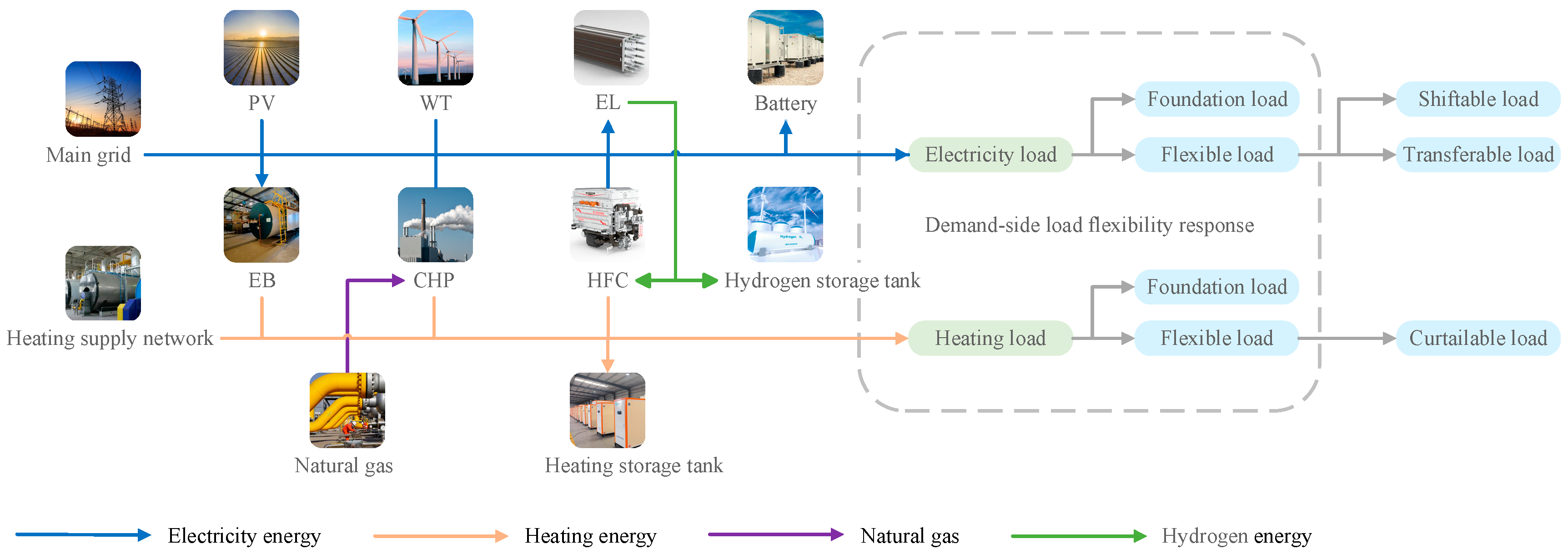
Based on the above research and analysis, this paper focuses on an IES with electricity–heat–hydrogen multi-energy coupling, composed of energy supply and conversion units including PV and WT generators, MTs, ELs, HFCs, electric boilers (EBs), energy storage devices, the power grid, gas network, and heating supply network. To address the uncertainties within the IES, the scenario method is employed to describe the uncertainties of renewable energy output and load. The integration of energy storage technology can, to some extent, stabilize the impacts caused by these uncertainties, and this technology has gradually become an indispensable part of IES [35,36]. Finally, a comprehensive norm is used to constrain the confidence level of uncertainty probabilities, constructing a two-stage RO model that accounts for the uncertainties of WT, PV, and loads. The first stage primarily focuses on long-term planning within the IES, including the selection and investment decisions for various energy equipment. The goal is to minimize the investment costs of the equipment while meeting future energy demands. The second stage shifts the focus to short-term operational optimization of the system, with the core objective of achieving real-time or near-real-time energy dispatch and balance. This involves coordinating the production, conversion, storage, and consumption of various energy sources, such as electricity, heat, and gas, across different time scales. In addition, to better alleviate peak electricity demand, further increase the utilization of renewable energy, and reduce phenomena such as wind curtailment and energy wastage, the price-based DR mechanism can fully leverage the control of loads to achieve reasonable energy utilization under multi-energy coordination. This mechanism optimizes the spatial and temporal distribution of demand-side energy loads. Studies have shown that integrating the DR mechanism into integrated IESs can significantly improve system operation efficiency and flexibility [37]. DR works by setting reasonable electricity prices, encouraging users to voluntarily adjust their electricity and heating behaviors. By incorporating energy storage devices, it achieves load peak shaving and valley filling, which not only saves energy costs for users but also alleviates the peak load pressure of IESs to some extent, reduces wind curtailment rates, and thus increases the utilization of wind power.

The structure of this article is as follows: The first part introduces the theoretical background, motivation for topic selection, and research objectives of this article; The second part establishes the model of the IES with electricity–heating–hydrogen cogeneration, which includes a DR model, system cost model, electricity–heating balance, and various equipment constraints; The third part establishes a data-driven DRO model, which includes the construction of uncertainty probability distribution sets, DRO models, solution processes, and overall model-solving steps; The fourth part verifies the effectiveness of the proposed model through numerical examples; Finally, the fifth part provides a brief summary and discussion.

The innovation of this article is mainly reflected in two aspects:

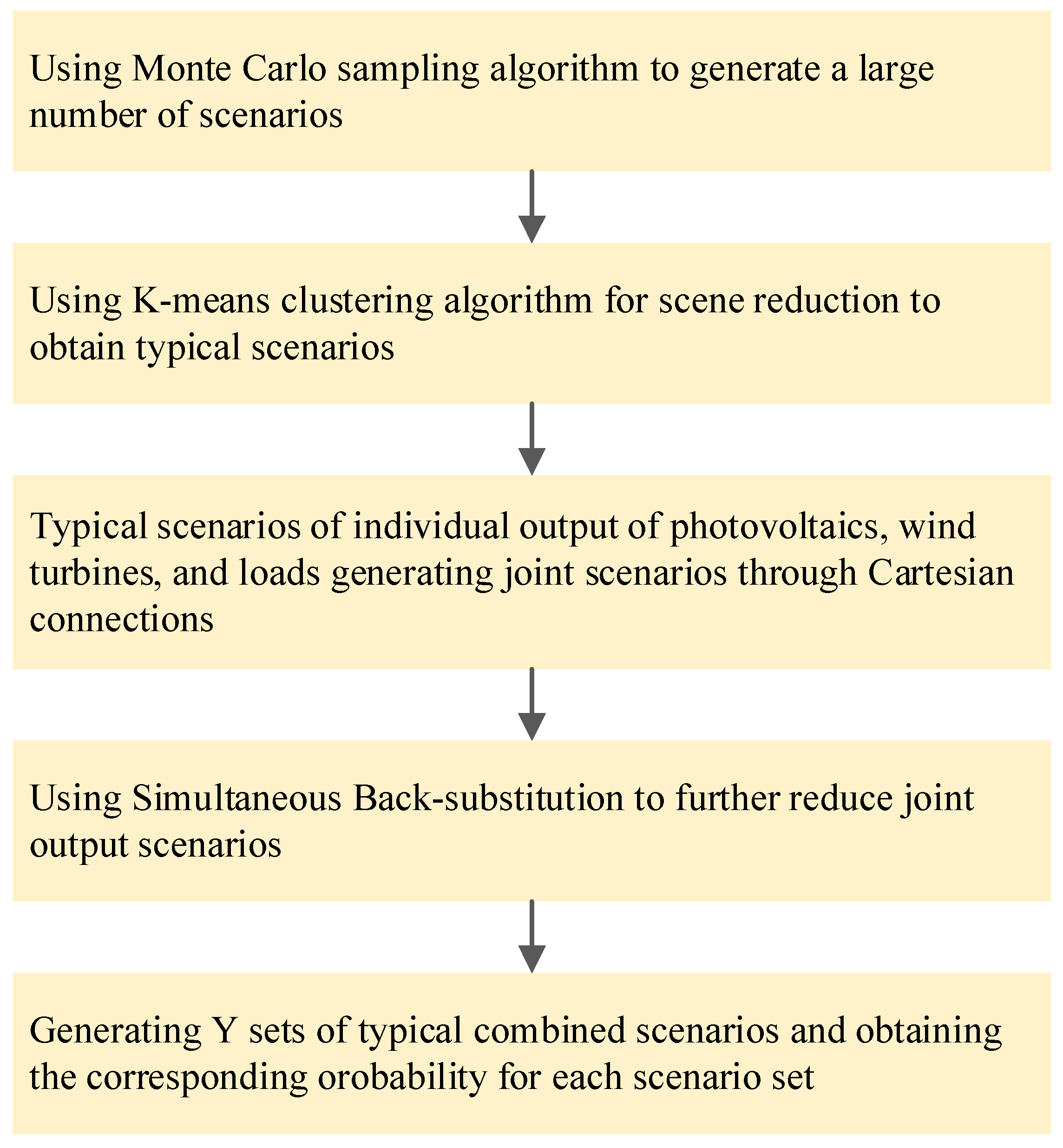
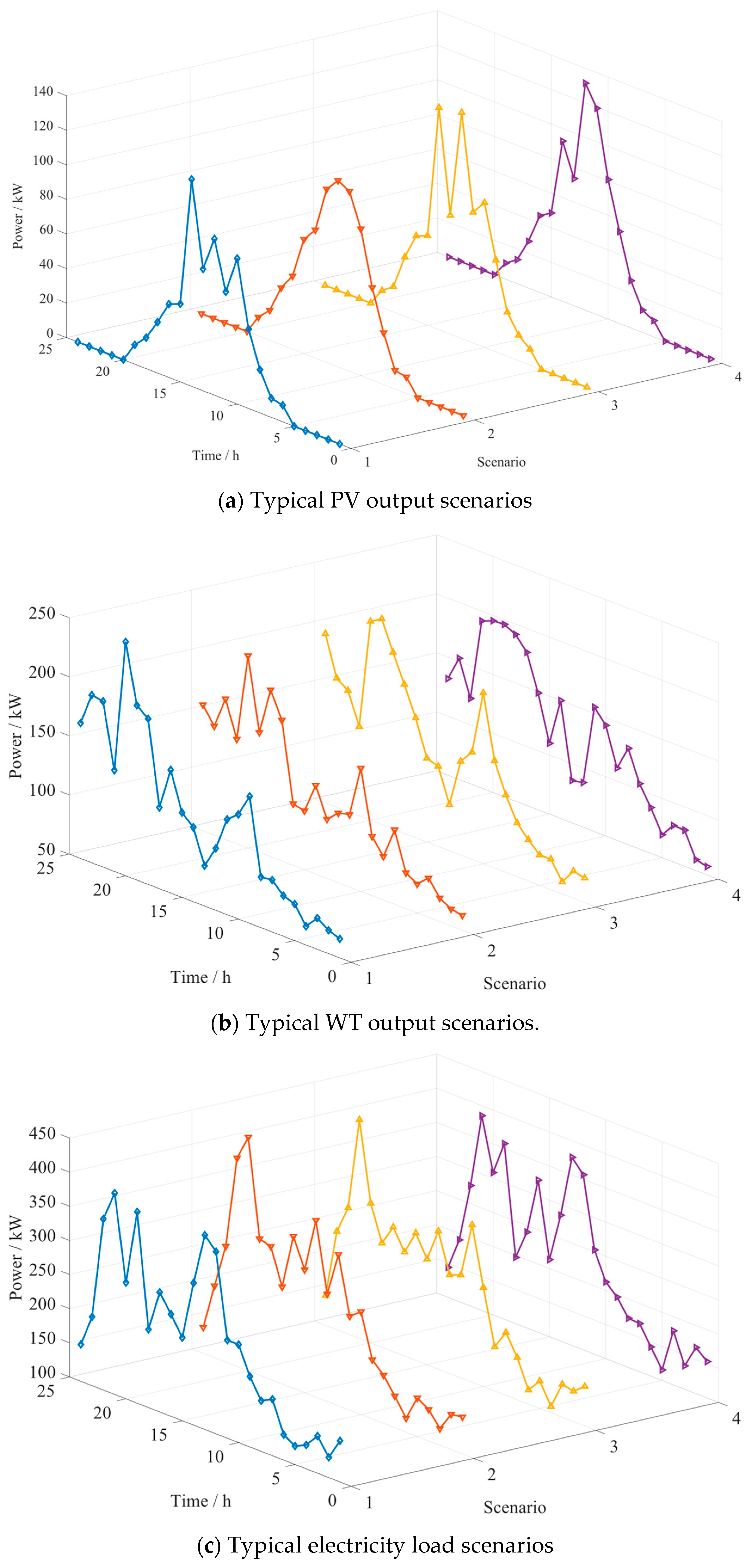
First, the use of typical scenarios obtained by combining the MC sampling method with the K-means clustering algorithm is proposed to describe the uncertainties in PV, WT, and loads. The MC, through completely random sampling, could capture extreme scenarios, such as extremely high or low PV and WT outputs, as well as load demand. This allows for testing the system’s performance under worst-case conditions, ensuring the reliability of the scheduling strategy, enhancing the model’s robustness, and mitigating the risk of high operational costs in practical applications. Distinguished from traditional approaches that focus on single energy sources or simplified scenarios, this method better aligns with the operational characteristics of complex real-world energy systems. Compared to other methods, such as Latin Hypercube Sampling (LHS), which is constrained by stratified sampling, it may result in insufficient scenario coverage, failing to adequately capture extreme scenarios; this limitation can lead to suboptimal model performance under extreme conditions, thereby increasing the risk of higher operational costs in practical applications.

Second, a two-stage DRO model is employed to address the uncertainties in PVs, WTs, and loads within the system, achieving a balance between economic efficiency and robustness in the optimization scheduling process. The master problem constructs the objective function by comprehensively considering multiple cost factors, including equipment operation, energy procurement, energy storage costs, curtailment costs of WT and PV power, DR compensations, and carbon emission costs. Additionally, strict constraints, such as equipment capacity limits, charging and discharging efficiency, and ramping constraints, are imposed to minimize the overall system cost. The subproblem focuses on addressing uncertainties, providing a reliable optimization framework for addressing complex energy environments and uncertainty management. It effectively balances the economic efficiency and robustness of the scheduling results. Additionally, by incorporating a DR operational mechanism, the distribution of electricity and heating loads is optimized, further enhancing system operation and reducing system operating costs.

2. IES Model

The structural diagram of the IES constructed in this article is shown in Figure 1. The energy supply part includes WT, PV, electricity purchased from the grid, gas purchased from the gas network, and heating energy purchased from the heating supply network. The energy conversion and storage parts includes EB, combined heat and power units (CHP), EL, HFC, batteries, heating storage tanks, and hydrogen storage tanks. Each device operates in coordination to meet the electricity and heating load requirements of the system under the DR mechanism.

2.1. DR Mechanism Model

The DR mechanism [38] refers to the process in which users autonomously adjust their electricity consumption behavior based on the load price signals provided by relevant authorities [39]. The DR model established in this article primarily includes three categories: shiftable loads, transferable loads, and reducible loads.

2.1.1. Shiftable Load

Shiftable load refers to the load that can be entirely shifted from one time period to another. The compensation required for the user after shifting is:

$$\left\{\begin{array}{l}{F}_{shift}=F_{\mathit{cos}t}^{shift}\cdot P_{total}^{shift}\cdot {\displaystyle \sum _{t=t_{sh-}}^{t_{sh+}-t_D+1}}{\varphi }_t\\ S_{shift}=[t_{sh},t_{sh+}-t_D+1]\cup \left\{t_s\right\}\\ H_{shift}=(0,...,P_{\tau }^{shift},P_{\tau +1}^{shift},...,P_{\tau +{\tau }_D-t_s}^{shift},\dots ,0)\\ {H^{*}}_{shift}=(0,\dots ,P_{t_s}^{shift},P_{t_s+1}^{shift},\dots ,P_{t_D}^{shift},\dots ,0)\end{array}\right.$$

(1)

where $F_{\mathit{cos}t}^{shift}$ is the compensation price per unit of shiftable load power, ¥/kW; $P_{total}^{shift}$ is the total shifted power of $H_{shift}$, in kW; ${\varphi }_t$ is the shifting status of $H_{shift}$ at time period $t$, with a value of 0 or 1; $S_{shift}$ is the set of starting time periods for load shifting; $H_{shift}$ is the power distribution vector of $H_{shift}^{*}$ shifted from the starting time period $t_s$ to the starting time period $\tau$, where no shifting occurs when $\tau =t_s$; and $H_{shift}^{*}$ is the power distribution vector before participating in the scheduling.

2.1.2. Transferable Load

Transferable load refers to the redistribution of a device’s total load across different time periods while ensuring that the overall load remains unchanged. The power constraint for load transfer is as follows:

$${\varpi }_t{P}_{min}^{tran}<P_t^{tran}<{\varpi }_t{P}_{max}^{tran}$$

(2)

where $P_{min}^{tran}$ and $P_{max}^{tran}$, respectively, are the minimum and maximum power of transferable load, in kW; $P_t^{tran}$ is the amount of load transferred at time period $t$; and ${\varpi }_t$ is the transfer status at time period $t$, with a value of 0 or 1.

To prevent excessive dispersion of a load that could lead to frequent start–stop cycles of equipment, constraints on the minimum continuous operation time of the transferable load need to be imposed. Considering the operation of transferable loads starting from time $t$, if ${\varpi }_t-{\varpi }_{t-1}=0$, then the operational state of the equipment associated with the transferable load remains unchanged at time $t$. If ${\varpi }_t-{\varpi }_{t-1}=1$, it indicates that the equipment begins load transfer at time $t$. Consequently, the total operational state of the equipment over the period from $t$ to $t+T_{min}^{tran}-1$ must satisfy the following condition:

$${\displaystyle \sum _{\tau =t}^{t+T_{min}^{tran}-1}}{\varpi }_t\ge T_{min}^{tran}$$

(3)

where $T_{min}^{tran}$ is the minimum continuous operation time, h.

In summary, the compensation cost after load transfer is:

$$F_{tran}=F_{\mathit{cos}t}^{tran}{\displaystyle \sum _{t=t_{tr-}}^{t_{tr+}}}\left({\varpi }_t{P}_t^{tran}\right)$$

(4)

where $F_{\mathit{cos}t}^{tran}$ is the compensation price per unit of transferable load power, ¥/kW.

2.1.3. Curtailable Load

The curtailable load fundamentally differs the shiftable and transferable loads. After adjustment, the total load of shiftable and transferable loads remains unchanged, while the curtailable load reduces the total load. The compensation cost after load reduction is:

$$\left\{\begin{array}{l}{F}_{cut}=F_{\mathit{cos}t}^{cut}{\displaystyle \sum _{t=1}^T}{\kappa }_t(P_t^{cut}-P_t^{cu{t}^{*}})\\ P_{\tau }^{cut}=(1-{\epsilon }_{\tau }{\kappa }_{\tau })P_{\tau }^{cu{t}^{*}}\end{array}\right.$$

(5)

where $F_{\mathit{cos}t}^{cut}$ is the compensation price per unit of curtailable load, ¥/kW; ${\kappa }_t$ is a binary variable indicating the reduction status of the curtailable load at time period $t$; $P_{\tau }^{cut}$ is the power at time period $\tau$ after participating in scheduling, in kW; $P_t^{cu{t}^{*}}$ is the power at time period $\tau$ before participating in scheduling, in kW; and ${\epsilon }_{\tau }$ is the load reduction coefficient at time period $\tau$.

To protect user rights, constraints on the number of reductions and the maximum and minimum continuous reduction times need to be imposed:

$$\left\{\begin{array}{l}{\displaystyle \sum _{t=1}^{24}}{\kappa }_t\le N_{max}\\ {\displaystyle \sum _{t=1}^{t+T_{max}^{cut}-1}}(1-{\kappa }_t)\ge 1\\ {\displaystyle \sum _{t=1}^{t+T_{min}^{cut}-1}}{\kappa }_t\ge T_{min}^{cut}\end{array}\right.$$

(6)

where $N_{max}$ is the maximum number of reductions; $T_{max}^{cut}$ is the maximum continuous reduction time, h; and $T_{min}^{cut}$ is the minimum continuous reduction time, h.

2.2. Cost Model of IES

The following objective function is established based on the structure diagram proposed in this article:

$$\left\{\begin{array}{c}{f}_{mp}=c_s{\displaystyle \sum _{t=1}^{T-1}}{u}_{t+1}^g\left(1-u_t^g\right)+c_{HFC}{\displaystyle \sum _{t=1}^{T-1}}{u}_{t+1}^{HFC}\left(1-u_t^{HFC}\right)\\ f_{sp}=c_{buy}+c_{h\_buy}+c_g+c_{cd}+c_{qw}+c_{q\nu }-c_{sell}+c_{dr}+c_{C{O}_2}\end{array}\right.$$

(7)

where $f_{mp}$ is the startup and shutdown costs of the MT and HFC; $c_s$ is the startup and shutdown cost coefficient of the MT; $u_t^g$ is the state variable of the MT at time $t$, which takes values of 0 or 1; $c_{HFC}$ is the start-up or shut-down cost coefficient of the HFC; $u_t^{HFC}$ is the state variable of the HFC at time $t$, with a value of either 0 or 1; $f_{sp}$ is the total operating costs of the system, in CNY; $c_{buy}$ is the costs of electricity purchased from the grid, in CNY; $c_{h\_buy}$ is the heat purchase costs from the thermal supply network, in CNY; $c_g$ is the natural gas costs required for CHP, in CNY; $c_{cd}$ is the energy storage costs, in CNY; $c_{qw}$ is the wind curtailment costs, in CNY; $c_{q\nu }$ is the solar curtailment costs, in CNY; $c_{sell}$ is the revenue from electricity sales, in CNY; $c_{dr}$ is the DR costs, in CNY; and $c_{C{O}_2}$ is the carbon emission costs, in CNY.

2.2.1. Cost of Electricity Purchased from the Grid

In the proposed model, the IES can conduct electricity transactions with the grid, and the transaction cost is:

$$c_{buy}=\sum _{t=1}^T{r}_t^{buy}\cdot P_t^{buy}$$

(8)

where $r_t^{buy}$ is the electricity purchase price of the IES from the grid at time $t$, in CNY; and $P_t^{buy}$ is the amount of electricity purchased by the IES from the grid at time $t$, in kWh.

2.2.2. Heat Purchase Cost from the Heating Supply Network

To provide users with a stable heating system, heat can be purchased from the heating network, and the heat purchase cost is:

$$c_{h\_buy}=\sum _{t=1}^T{r}_t^{h\_buy}\cdot P_t^{h\_buy}$$

(9)

where $r_t^{h\_buy}$ is the heat purchase price from the heating supply network at time $t$, in CNY; and $P_t^{h\_buy}$ is the heat purchase amount from the heating supply network at time $t$, in kWh.

2.2.3. Natural Gas Cost Required for CHP

To meet the user’s demand of electricity and heating load, natural gas needs to be purchased from the gas network. The purchase cost is:

$$c_g=\sum _{t=1}^T{r}_g\cdot P_{g,t}^{CHP}$$

(10)

where $r_g$ is the natural gas purchase price of the IES from the gas network, in CNY; and $P_{g,t}^{CHP}$ is the amount of natural gas purchased by the IES from the gas network at time $t$, in kWh.

2.2.4. Energy Storage Cost

Considering that energy storage equipment will incur depreciation during its use, the cost model is:

$$c_{cd}=\sum _{t=1}^T\left[r_{cde}\left(P_t^{che}+p_t^{dische}\right)+r_{cdh}\left(P_t^{chh}+p_t^{dischh}\right)+r_{cdH}\left(P_t^{chH}+p_t^{dischH}\right)\right]$$

(11)

where $r_{cde}$ is the degradation coefficient of electricity energy storage; $r_{cdh}$ is the degradation coefficient of heating energy storage;$r_{cdH}$ is the degradation coefficient of hydrogen energy storage; $P_t^{che}$ is the charging power of the electricity storage device, in kW; $p_t^{dische}$ is the discharging power of the electricity storage device, in kW; $P_t^{chh}$ is the charging power of the heating storage device, in kW;$p_t^{dischh}$ is the discharging power of the heating storage device, in kW; $P_t^{chH}$ is the charging power of the hydrogen storage device, in kW; and $p_t^{dischH}$ is the discharging power of the hydrogen storage device, in kW.

2.2.5. Wind and Solar Curtailment Costs

$$c_{qw}=\sum _{t=1}^T{r}_{qw}({\widehat{P}}_t^w-P_t^w)$$

(12)

$$c_{qv}=\sum _{t=1}^T{r}_{qv}({\widehat{P}}_t^v-P_t^v)$$

(13)

where $r_{qw}$ is the operating cost coefficient of the WT; ${\widehat{P}}_t^w$ is the wind power forecast at time $t$, in kW; $P_t^w$ is the actual wind power participating at time $t$, in kW; $r_{qv}$ is the operating cost coefficient of the PV; ${\widehat{P}}_t^v$ is the PV power forecast at time $t$, in kW; and $P_t^v$ is the actual PV power participating at time $t$, in kW.

2.2.6. Revenue from Electricity Sales

When there is excess electricity, the surplus can be sold to the grid. The revenue model is:

$$c_{sell}=\sum _{t=1}^T{r}_{sell}\cdot P_t^{sell}$$

(14)

where $r_{sell}$ is the electricity selling price of the IES to the grid, in CNY; and $P_t^{sell}$ is the amount of electricity selling to the grid by the IES at time $t$, in kWh.

2.2.7. DR Cost

The shiftable, transferable, and curtailable loads require corresponding compensation to be provided to the users:

$$c_{dr}=F_{shift}+F_{tran}+F_{cut}$$

(15)

where $F_{shift}$ is the compensation cost after load shifting, in CNY; $F_{tran}$ is the compensation cost after load transfer, in CNY; and $F_{cut}$ is the compensation cost after load reduction, in CNY.

2.2.8. Carbon Emission Cost

$$c_{C{O}_2}=\sum _{t=1}^{24}{\lambda }_{{CO}_2}{(\mu }_{grid}\cdot P_t^{buy}+{(\mu }_{gas}\cdot P_{g,t}^{CHP})$$

(16)

where ${\lambda }_{{CO}_2}$ is the carbon price, in CNY/ton CO₂;${ \mu }_{grid}$ is the carbon emission intensity of the power grid, in gCO₂/kWh; and ${\mu }_{gas}$ is the carbon emission intensity of natural gas, in gCO₂/kWh.

2.2.9. Operating Constraints of the EL

$$\left\{\begin{array}{c}{P}_{H_2,t}^{EL}={\eta }_{EL}\cdot P_{e,t}^{EL}\\ {u_t^{EL}\cdot P}_{e,EL}^{min}\le P_{e,t}^{EL}\le u_t^{EL}\cdot P_{e,EL}^{max}\end{array}\right.$$

(17)

where $P_{H_2,t}^{EL}$ and $P_{e,t}^{EL}$ are the output hydrogen power and input electrical power of the EL at time t, respectively, in kW; ${\eta }_{EL}$ is the power-to-hydrogen conversion efficiency; $u_t^{EL}$ is the start-up/shut-down state at time t; and $P_{e,EL}^{max}$ and $P_{e,EL}^{min}$ are the upper and lower limits of electrical power consumption, respectively, in kW.

2.2.10. Operating Constraints of the HFC

$$\left\{\begin{array}{c}{P}_{e,t}^{HFC}={\eta }_{HFC}\cdot P_{H_2,t}^{HFC}\\ {u_t^{HFC}\cdot P}_{H_2,HFC}^{min}\le P_{H_2,t}^{HFC}\le u_t^{HFC}\cdot P_{H_2,HFC}^{max}\\ {\omega }_{HFC}^{min}\le P_{h,t}^{HFC}/P_{e,t}^{HFC}\le {\omega }_{HFC}^{max}\end{array}\right.$$

(18)

where $P_{e,t}^{HFC}$ and $P_{H_2,t}^{HFC}$ are the output electrical power and input hydrogen power of the HFC at time t, respectively, in kW; $P_{h,t}^{HFC}$ is the output thermal power at time $t$; ${\eta }_{EL}$ is the hydrogen-to-electricity conversion efficiency of HFC; $P_{H_2,HFC}^{max}$ and $P_{H_2,HFC}^{min}$ are the upper and lower limits of hydrogen power consumption, respectively, in kW; and ${\omega }_{HFC}^{max}$ and ${\omega }_{HFC}^{min}$ are the upper and lower limits of the heat-to-power ratio of HFC, respectively.

2.3. Restraints and Balance

2.3.1. PV and WT Constraints

$$\left\{\begin{array}{c}0\le P_t^w\le P_w^{max}\\ 0\le P_t^{\nu }\le P_{\nu }^{max}\end{array}\right.$$

(19)

where $P_w^{max}$ is the maximum output power of the WT, in kW; and $P_{\nu }^{max}$ is the maximum output power of the PV system, in kW.

2.3.2. Energy Purchase and Sale Constraints from External Energy Networks

$$\left\{\begin{array}{c}{P}_{buy}^{min}\le P_t^{buy}\le P_{buy}^{max}\\ P_{sell}^{min}\le P_t^{sell}\le P_{sell}^{max}\\ P_{h\_net}^{min}\le P_t^{h\_buy}\le P_{h\_net}^{max}\\ P_g^{min}\le P_{g,t}^{CHP}\le P_g^{max}\end{array}\right.$$

(20)

where $P_{buy}^{min}$ and $P_{buy}^{max}$ are the lower and upper limits of electricity purchase by the IES from the external power grid, respectively; $P_{sell}^{min}$ and $P_{sell}^{max}$ are the lower and upper limits of electricity sale by the IES to the external power grid, respectively; $P_{h\_net}^{min}$ and $P_{h\_net}^{max}$ are the lower and upper limits of heat purchase by the IES from the external heating supply network, respectively; and $P_g^{min}$ and $P_g^{max}$ are the lower and upper limits of gas purchase by the IES from the external gas network, respectively.

2.3.3. Operating Constraints of the EB

$$\left\{\begin{array}{c}{P}_{\mathrm{h},t}^{EB}={\eta }_{EB}\cdot P_{e,t}^{EB}\\ {u_t^{EB}\cdot P}_{e,EB}^{min}\le P_{e,t}^{EB}\le u_t^{EB}\cdot P_{e,EB}^{max}\end{array}\right.$$

(21)

where $P_{\mathrm{h},t}^{EB}$ and $P_{e,t}^{EB}$ are the output thermal power and input electrical power of the EB at time $t,\mathrm{r}\mathrm{e}\mathrm{s}\mathrm{p}\mathrm{e}\mathrm{c}\mathrm{t}\mathrm{i}\mathrm{v}\mathrm{e}\mathrm{l}\mathrm{y}$, in kW; ${\eta }_{EB}$ is the electric-thermal conversion efficiency; $u_t^{EB}$ is the start-up/shut-down state at time $t$; and $P_{e,EB}^{min}$ and $P_{e,EB}^{max}$ are the lower and upper limits of electrical power consumption, respectively, in kW.

2.3.4. CHP Operating Constraints

$$\left\{\begin{array}{c}{P}_{e,t}^{CHP}={\omega }_{g2e}\cdot P_{g,t}^{CHP}\\ P_{g,CHP}^{min}\le P_{g,t}^{CHP}\le P_{g,CHP}^{max}\\ {\omega }_{CHP}^{min}\le {\omega }_{h/e}\le {\omega }_{CHP}^{max}\end{array}\right.$$

(22)

where $P_{e,t}^{CHP}$ is the electricity output power of the CHP system at time $t$, in kW; ${\omega }_{g2e}$ is the gas-to-electricity conversion efficiency of the $CHP$ unit; $P_{g,t}^{CHP}$ is the input gas power to the CHP system at time $t$, in kW; $P_{g,CHP}^{max}$ is the upper limit of the input gas power to the CHP system, in kW; $P_{g,CHP}^{min}$ is the lower limit of the input gas power to the CHP system, in kW; ${\omega }_{h/e}$ is the heating-to-electricity ratio of the CHP unit; ${\omega }_{CHP}^{max}$ is the upper limit of the heating-to-electricity ratio of the CHP system; and ${\omega }_{CHP}^{min}$ is the lower limit of the heating-to-electricity ratio of the CHP system.

2.3.5. Ramp-Up Constraints

$$\left\{\begin{array}{c}{P}_{g,t}^{CHP}-P_{g,t-1}^{CHP}\le {\gamma }_{u\_g}\cdot \left(1-u_{t-1}^g\right)+P_{g,CHP}^{max}\cdot u_t^g\\ P_{g,t-1}^{CHP}-P_{g,t}^{CHP}\le {\gamma }_{d\_g}\cdot \left(1-u_t^g\right)+P_{g,CHP}^{max}\cdot u_{t-1}^g\\ P_{e,t}^{EL}-P_{e,t-1}^{EL}\le {\gamma }_{u\_EL}\cdot \left(1-u_{t-1}^{EL}\right)+P_{e,EL}^{max}\cdot u_t^{EL}\\ P_{e,t-1}^{EL}-P_{e,t}^{EL}\le {\gamma }_{d\_EL}\cdot \left(1-u_t^{EL}\right)+P_{e,EL}^{max}\cdot u_{t-1}^{EL}\\ P_{H_2,t}^{HFC}-P_{H_2,t-1}^{HFC}\le {{\gamma }_{u\_HFC}\cdot \left(1-u_{t-1}^{HFC}\right)+P}_{H_2,HFC}^{max}\cdot u_t^{HFC}\\ P_{H_2,t-1}^{HFC}-P_{H_2,t}^{HFC}\le {{\gamma }_{d\_HFC}\cdot \left(1-u_t^{HFC}\right)+P}_{H_2,HFC}^{max}\cdot u_{t-1}^{HFC}\end{array}\right.$$

(23)

where ${\gamma }_{u\_g}$ is the ramp-up rate upper limit of the CHP unit; ${\gamma }_{d\_g}$ is the ramp-up rate lower limit of the CHP unit; ${\gamma }_{u\_EL}$ is the ramp-up rate upper limit of the EL unit; ${\gamma }_{d\_EL}$ is the ramp-up rate lower limit of the EL unit; ${\gamma }_{u\_HFC}$ is the ramp-up rate upper limit of the HFC unit; and ${\gamma }_{d\_HFC}$ is the ramp-up rate lower limit of the HFC unit.

2.3.6. Energy Storage Operating Constraints

The following constraints are added to the energy storage device’s operation process, including SOC status, charge and discharge status, and energy scheduling start and end status:

$$\left\{\begin{array}{c}0\le P_t^{ch}\le u_t^{ch}\cdot P_{cd}^{max}\\ 0\le P_t^{dis}\le u_t^{dis}\cdot P_{cd}^{max}\\ u_t^{ch}\cdot u_t^{dis}=0\\ S_{min}\le S_t\le S_{max}\\ S_t=S_{t-1}+{\omega }_{ch}\cdot P_t^{ch}-{\omega }_{disch}\cdot P_t^{disch}\end{array}\right.$$

(24)

where $P_t^{ch}$ is the charging power of the energy storage device at time $t$, in kW; $P_t^{dis}$ is the discharging power of the energy storage device at time $t$, in kW; $u_t^{ch}$ is charging status at time $t$, with values of 0 or 1; $u_t^{dis}$ is discharging status at time $t$, with values of 0 or 1; $P_{cd}^{max}$ is the upper limit of charging and discharging power for energy storage, in kW; $S_t$ is capacity of the energy storage at time $t$, in kW; $S_{min}$ is the lower limit capacity of the energy storage, in kW; $S_{max}$ is the upper limit capacity of the energy storage, in kW; ${\omega }_{ch}$ is the charging efficiency of the energy storage; and ${\omega }_{disch}$ is the discharging efficiency of the energy storage.

2.3.7. Electricity Power Balance Constraints

$$\begin{gathered} \sum _{t=1}^{24}\left(P_{e,t}^{HFC}+P_t^{buy}+P_{e,t}^{CHP}+{\omega }_{disch}\cdot P_t^{dische}+P_t^w+P_t^{\nu }\right) \\ =\sum _{t=1}^{24}\left(P_t^{le}+P_t^{shift}+P_t^{tran}+P_t^{sell}+{\omega }_{ch}\cdot P_t^{che}+P_{e,t}^{EL}+P_t^{EB}\right) \end{gathered}$$

(25)

where $P_t^{le}$ is the electricity load at time $t$, in kW; $P_t^{shift}$ is the shiftable electricity load at time $t$, in kW; and $P_t^{tran}$ is the transferable electricity load at time $t$, in kW.

2.3.8. Heating Power Balance Constraints

$$\begin{gathered} \sum _{t=1}^{24}\left((1-{\eta }_{loss}^{h\_net})\cdot P_t^{h\_buy}+P_{h,t}^{HFC}+{\omega }_{h/e}\cdot P_{e,t}^{CHP}+P_{h,t}^{EB}+{\omega }_{disch}\cdot P_t^{dischh}\right) \\ =\sum _{t=1}^{24}\left(P_t^{lh}-P_t^{cut}+{\omega }_{ch}\cdot P_t^{chh}\right) \end{gathered}$$

(26)

where $P_t^{lh}$ is the heating load at time $t$, in kW; $P_t^{cut}$ is the reducible heating load at time $t$, in kW; and ${\eta }_{loss}^{h\_net}$ is the heat loss efficiency of the heating supply network.

2.3.9. Hydrogen Power Balance Constraints

$$\sum _{t=1}^{24}\left(P_{H_2,t}^{EL}{\cdot \eta }_{HFC}+{\omega }_{disch}\cdot P_t^{dische}\right)=\sum _{t=1}^{24}\left(P_{H_2,t}^{HFC}+{\omega }_{ch}\cdot P_t^{che}\right)$$

(27)

3. Data-Driven DRO Model

3.1. Construction of Uncertainty Probability Distribution Set

To address the uncertainties in PV, WT, and electricity–heating loads within the IES, multiple representative scenarios of PV, WT, and loads output are generated along with their probability distributions. These uncertainties are incorporated into the optimization model to ensure that the scheduling strategy can effectively accommodate the stochastic variations in renewable energy generation and load demand. This approach enhances the system’s capability to integrate renewable energy and improves the robustness of its operation.

3.1.1. Distribution Function and Multi-Scenarios Generation Method

In the optimization scheduling of an IES, the modeling of uncertainties in PV, WT, and load demand is one of the core challenges. Based on the historical data characteristics of PV generation, WT generation, and electricity–heating loads, this article employs MC random sampling to generate multiple scenarios. Additionally, the following probability distribution models are incorporated to comprehensively capture the uncertainty space:

(1)

PV power output modeling: Beta distribution

PV power output is significantly influenced by weather conditions such as solar irradiance and cloud cover, with its normalized power values typically distributed within the range of [0, 1]. Therefore, a Beta distribution is selected to characterize the probabilistic properties of PV power output. Its probability density function is given by:

$$f(x;\alpha ,\beta )={\displaystyle \frac{x^{\alpha -1}(1-x{)}^{\beta -1}}{B(\alpha ,\beta )}},0<x<1$$

(28)

Among them, $\alpha >0$, $\beta >0$ are the two shape—parameters that can be fitted using historical data to adjust the distribution’s shape, such as symmetry and skewness; and $B(\alpha ,\beta )$ is the Beta function. Its calculation formula is $B(\alpha ,\beta )={\displaystyle \frac{\Gamma \left(\alpha \right)\Gamma \left(\beta \right)}{\Gamma (\alpha +\beta )}}$; the gamma function $\Gamma (·)$ satisfies $\Gamma \left(n\right)=(n-1)!$ in the integer domain, which supports efficient computation of the parameter.

(2)

WT power output modeling: Weibull distribution

WT power output is closely related to wind speed, which typically follows a Weibull distribution. Its probability density function is expressed as:

$$f(x;\lambda ,k)=\left\{\begin{array}{l}{\displaystyle \frac{k}{\lambda }}({\displaystyle \frac{x}{\lambda }}{)}^{k-1}{e}^{-({\displaystyle \frac{x}{\lambda }}{)}^k},x\ge 0\\ 0,x<0\end{array}\right.$$

(29)

Among them, $\lambda$is the scale parameter, which determines the typical range of wind speed and reflects the characteristic of “average wind speed”; and $k$ is the shape parameter. When $k=1$, the Weibull distribution degenerates into an exponential distribution. When $k=2,$ the Weibull distribution resembles a Rayleigh distribution, allowing it to flexibly adapt to wind speed characteristics across different regions.

(3)

electricity–heating loads power output modeling: normal distribution

The uncertainty in load demand is typically influenced by multiple factors, such as user behavior and temperature variations. Its forecasting error follows a normal distribution. The probability density function is expressed as:

$$f(x)={\displaystyle \frac{1}{\sqrt{2\pi }\sigma }}{e}^{-{\displaystyle \frac{(x-\mu {)}^2}{2{\sigma }^2}}},-\infty <x<+\infty$$

(30)

Among them, $\mu$ represents the expected value of the load, reflecting the typical energy consumption pattern, while $\sigma$ describes the range of load fluctuations. The larger $\sigma$ is, the higher the uncertainty.

Based on the aforementioned probability distribution models, the MC random sampling algorithm is employed to generate multiple scenarios for four types of random variables: PV power output, WT generation, and electricity–heating loads. This involves drawing a large number of random samples from each distribution, aiming to comprehensively cover the potential variations in WT and PV output, as well as load demand, ensuring the representativeness and diversity of the scenarios.

3.1.2. Scenario Clustering

Due to the scenarios generated by MC sampling are relatively large, directly using them for optimization calculations would result in extremely high computational complexity. Therefore, the K-means clustering algorithm is applied to compress the sampled scenarios and extract a set of representative scenarios. When determining the number of clusters, a larger number is not always better. If the number of clusters is too high, it may lead to a decrease in the optimization model’s computational speed. Therefore, an appropriate number of clusters needs to be selected based on the data themselves. In this article, the silhouette coefficient method is used to determine the number of scenario clusters.

As shown in Figure 2, based on the large number of scenarios generated by MC sampling, the K-means clustering algorithm is used to reduce the scenarios into a limited set of scenarios with distinct probabilities for PV units, WT, electricity loads, and heating loads. These four types of scenarios are then combined using the Cartesian product. The SBR technique is applied for further scenario reduction, ultimately obtaining Y sets of representative joint output scenarios for PV, WT, and loads, along with their corresponding probabilities. Subsequently, the objective function value for each joint scenario can be calculated and summed, facilitating system analysis.

3.2. DRO Model

Given the potential limitations of historical forecast data on PV, WT, and loads, the representative scenarios obtained through scenario clustering may not fully capture actual fluctuations. To address this, a DRO approach is introduced, where the representative scenarios serve as inputs. A distributional ambiguity set is defined using comprehensive norm constraints to restrict the fluctuation range of probability distributions, thence between robustness and economic efficiency in the optimization process.

The two-stage DRO model developed in this article can be summarized as follows:

The first stage establishes the foundation for the normal operation of the system and performs preliminary cost optimization by minimizing fixed costs. Its objective function comprehensively considers various cost components, such as operational costs, compensation costs, and the variable $\eta$ associated with uncertainties. The second stage focuses on adjusting decisions based on uncertainty scenarios. Specifically, it calculates the system’s cost or revenue under different uncertainty scenarios according to the first-stage decisions and the realization of uncertain variables. This information is then fed back to the first stage to refine the decision variables, aiming to minimize the expected adjustment cost in the worst-case scenario. The matrix representation of the data-driven two-stage DRO model is as follows:

$$\underset{x\in X}{min\left\{m^{T}x\right\}}+\underset{p_b\in {\Omega }_b}{max}\left\{{\displaystyle \sum _{b=1}^{N_b}}{p}_b\underset{y_b\in Y(x,{\xi }_b)}{min}\left\{n^T{y}_b+k{\xi }_b\right\}\right\}$$

(31)

$$s.t.Cx\le c$$

(32)

$$D{y}_b\le d{\xi }_b$$

(33)

$$Gx+H{y}_b\le g_b$$

(34)

$$Ax+B{y}_b=q_b$$

(35)

where $x$ is the first-stage variable; $y_b$ is the second-stage variable; $m$ and $n$ are the cost coefficients corresponding to the first and second-stage variables; ${\Omega }_b$ is the set that $p_b$ satisfies; $\underset{p_b\in {\Omega }_b}{max}$ is the scenario probability distribution value that maximizes the objective function; $k$ is the penalty coefficient per unit deviation; ${\xi }_b$ is the vector of actual wind and photovoltaic output deviations and load fluctuations in scenario $b$; $N_b$ is the number of scenario clusters; $p_b$ is the occurrence probability of scenario $b$; $C,c,D,d,G,H,g_b,A,B,q_b$ are the matrices or vectors that match the variables in the constraint conditions of the optimization model; Equation (32) is all the constraints related to the first-stage variables; Equation (33) is the relevant constraints of the second-stage variables; and Equations (34) and (35) are the coupling constraints of the two-stage variables, such as the system power balance constraints, among others.

To balance robustness and economic efficiency in the optimization process while ensuring that the actual probability distribution fluctuates within a reasonable range and aligns more closely with real data characteristics, 1-norm [12] and ∞-norm [40] constraints are introduced to limit the fluctuation range of probability distributions for scenarios. This ensures that the optimization model remains robust even under the worst-case probability distribution. Specifically, by imposing constraints based on the 1-norm and ∞-norm, a distributional ambiguity set is defined, encompassing multiple possible probability distributions. This distributional ambiguity set reflects the uncertainty in the perception of probabilistic distributions of uncertain factors. While the exact occurrence probability of each scenario cannot be precisely determined, comprehensive norm constraints can be used to define a reasonable fluctuation range for the probability distribution, mitigating scenario deviations caused by limitations in historical data. During the optimization process, by minimizing the expected cost under the worst-case distribution, the model effectively balances economic efficiency and robustness, thereby reducing the impact of extreme scenarios on system operating costs. If only considering the 1-norm or ∞-norm separately, it may lead to extreme or biased probability fluctuations. Therefore, a comprehensive norm constraint is constructed, ensuring that the distributional ambiguity set ${\Omega }_b={\Omega }_1+{\Omega }_{\infty }$ satisfies the following constraints:

$${\Omega }_b=\left\{\{p_b\}\left|\begin{array}{c}{p}_b\ge 0,b=\mathrm{1,2},...,N_b\\ {\displaystyle \sum _{b=1}^{N_b}}{p}_b=1\\ {\displaystyle \sum _{b=1}^{N_b}}\left|p_b\left.-p_b^0\right|\le {\theta }_1\right.\\ \underset{1\le b\le N_b}{max}\left|p_b\left.-p_b^0\right|\le {\theta }_{\infty }\right.\end{array}\right.\right.$$

(36)

where $p_b^0$ is the reference probability distribution value of representative scenario $b$; ${\theta }_1$ and ${\theta }_{\infty }$ are the constraint radius, which is the allowable deviation under the corresponding norm constraint; and $N_b$ is the number of typical scenarios.

As stated in reference [12], the deviation of scenario probabilities satisfies the following probabilistic guarantee:

$$\left\{\begin{array}{l}{P}_r\{{\displaystyle \sum _{b=1}^{N_b}}\left|p_b\right.\left.-p_b^0\right|\le {\theta }_1\}\ge 1-2N_b{e}^{{\displaystyle \frac{-2M{\theta }_1}{N_b}}}\\ P_r\{\underset{b=\mathrm{1,2},...N_b}{max}\left|p_b\right.\left.-p_b^0\right|\le {\theta }_{\infty }\}\ge 1-2N_b{e}^{-2M{\theta }_{\infty }}\end{array}\right.$$

(37)

where $p_r$ represents the probability that the event within the parentheses holds; and $M$ is the number of historical scenarios.

Let the right-hand side of Equation (37) be equal to ${\alpha }_1$ and ${\alpha }_{\infty },$ respectively, then it is transformed into the following equation:

$$\left\{\begin{array}{l}{\theta }_1={\displaystyle \frac{N_b}{2M}}\mathit{ln}{\displaystyle \frac{2N_b}{1-{\alpha }_1}}\\ {\theta }_{\infty }={\displaystyle \frac{1}{2M}}\mathit{ln}{\displaystyle \frac{2N_b}{1-{\alpha }_{\infty }}}\end{array}\right.$$

(38)

where ${\alpha }_1$ and ${\alpha }_{\infty }$ represent the confidence levels that the probability distribution is required to satisfy.

It can be seen from Equations (36) to (38) that as the amount of historical data increases, the value of $\theta$ decreases, which means that the confidence set at the same confidence level will shrink. When the historical data increases to infinity, both ${\theta }_1$ and ${\theta }_{\infty }$ decrease to 0, indicating that the initial distribution is the true distribution.

4. Solution Process

For the min–max–min three-layer optimization model established in Equation (31), this article decomposes it into two parts—the master problem and the subproblem—and then employs a decomposition algorithm based on Column and Constraint Generation (C&CG) to solve it. By iteratively solving the master problem and the subproblem using the C&CG algorithm, the upper and lower bounds are progressively tightened until an optimal solution that meets a certain precision requirement is obtained, at which point the iteration stops.

4.1. Master Problem

The master problem can be expressed in the form of matrix:

$$\left\{\begin{array}{c}L=\underset{x\in X,,y_b^i\in Y(x,{\xi }_{b)},\eta }{min}(m^{T}x+\eta )\\ s.t.\eta \ge \underset{p_b\in {\Omega }_b}{max}{\displaystyle \sum _{b=1}^{N_b}}{p}_b^i\underset{y_b^i\in Y(x,{\xi }_b)}{min}(n^T{y}_b^i+k{\xi }_b),\forall i=\mathrm{1,2},...,I\\ Cx\le c\\ D{y}_b^i\le d{\xi }_b,\forall b,\forall i=\mathrm{1,2},...,I\\ Gx+H{y}_b^i\le g_b,\forall b,\forall i=\mathrm{1,2},...,I\\ Ax+B{y}_b^i=q_b,\forall b,\forall i=\mathrm{1,2},...,I\end{array}\right.$$

(39)

where $\eta$ is the given threshold; and $I$ is the total number of model iterations.

4.2. Sub-Problem

The sub-problem is a double-layer structure of max–min, which is solved after the first stage variable $x^{*}$ is given, and is expressed in matrix form as:

$$\underset{p_b\in {\Omega }_b}{max}{\displaystyle \sum _{b=1}^{N_b}}{p}_b^i\underset{y_b^i\in Y(x,{\xi }_b)}{min}(n^T{y}_b^i+k{\xi }_b),\forall i=\mathrm{1,2},...,I$$

(40)

From Equation (40), it can be observed that in the sub-problem, the probability values of discrete scenarios exhibit an uncorrelated relationship with other variables. Therefore, the sub-problem can be decomposed into two steps for solution: first, solving the inner minimization problem, and then addressing the outer maximization problem. This process is explicitly shown in the following equation:

$$\left\{\begin{array}{c}{u}_b=\underset{y_b\in Y(x,{\xi }_b)}{min}(n^T{y}_b^i+k{\xi }_b)\\ U=\underset{p_b\in {\Omega }_b}{max}{\displaystyle \sum _{b=1}^{N_b}}{p}_b\cdot u_b\end{array}\right.$$

(41)

where $u_b$ can be obtained from the solution result of the master problem.

4.3. Model-Solving Steps

To sum up, the specific solution process of the model is shown in Figure 3:

5. Example Analysis

5.1. Example Description

In this section, a certain community IES is selected as the research object. Taking the system structure shown in Figure 1 as an example, the effectiveness of the proposed model and algorithm is verified through case-based simulation. The simulation is carried out using MATLAB 2018a simulation software, and the cplex solver is called by yalmip. The time-of-use electricity price, gas price, and the model parameters of each device are shown in

Table 1. Time-of-use electricity price and natural gas price.

Category	Gas Price	Price/(CNY/kWh) (Electricity/Heating), (CNY/m3) (Gas)
Electricity price	01:00~07:00, 23:00~24:00	0.38
	08:00~11:00, 15:00~18:00	0.68
	12:00~14:00, 19:00~22:00	1.20
Heating price	00:00~05:00, 10:00~13:00	0.67
	05:00~08:00, 15:00~24:00	0.48
	08:00~10:00, 13:00~15:00	0.28
Gas price	All-day	0.35

,

Table 2. Parameter setting of energy conversion equipment.

Equipment Name	Energy Conversion Efficiency	Capacity/kW
CHP	0.92	300
EB	0.90	250
EL	0.87	200
HFC	0.95	250

and

Table 3. Parameter setting of energy storage device.

Equipment Name	Capacity Lower—Bound Constraint	Capacity Upper—Bound Constraint	Capacity/kW	Charge—Discharge Efficiency
Battery	0.1	0.9	400	0.95
Heating storage tank	0.1	0.9	300	0.95
Hydrogen storage tank	0.1	0.9	300	0.95

. The solution process of the model in this article is shown in Figure 3. PV, WT, and loads forecasting data are cited from Reference [38]. In this article, based on the 1000 PV, WT, and loads output data generated by MC, the clustering method is used to obtain the typical scenarios. The number of typical scenarios is set to 4, and the confidence levels ${\alpha }_1$ and ${\alpha }_{\infty }$ are both 80%.

5.2. Scenario Generation Analysis

In the experiment, utilizing MC simulation based on different distribution functions, 1000 sets of initial scenario data for PV, WT, and loads were generated. The K-means clustering algorithm was employed to reduce these to 20 scenarios with varying probabilities for PV units, WT units, electricity load, and heating load, each considered separately. These four types of scenarios were then combined using a Cartesian product, and the SBR technique was applied to further reduce the number of scenarios. Ultimately, four typical combined output scenarios for PV, WT, electricity load, and heating load were obtained, as illustrated in Figure 4.

From the PV, WT, and electricity–heating loads scenarios distributions shown in Figure 4, it can be observed that scenarios data are relatively dispersed across different time periods and scenario indices. Taking PV output as an example, the numerical differences among different scenarios, represented by various colored curves, are significant at different time steps, covering a broad range. This dispersion indicates that the MC sampling method effectively captures a wide variety of potential situations, reflecting greater uncertainty and variability. Since these parameters exhibit diverse and stochastic variations in actual operation, this approach provides an advantage in accurately simulating the complex joint output of PV, WT, and load conditions.

The range of output values also varies among scenarios. Some scenarios exhibit a relatively wide fluctuation range, potentially spanning from lower to higher power outputs, while others have a narrower range of fluctuations, indicating more stable or smaller variations. This further demonstrates the representativeness of the reduced scenarios in reflecting the overall diversity of scenarios, encompassing both highly variable and relatively stable conditions.

The curves of scenario data exhibit significant variability. For instance, the electricity load scenarios show pronounced fluctuations, reflecting the rapid changes and uncertainties in load demand at different times. This high level of volatility aligns more closely with the real-world characteristics of load variations, enabling a more realistic simulation of system operations under different load fluctuation conditions.

The probabilities of each scenario are listed in

Table 4. The corresponding probabilities for the four typical scenarios are as follows.

Scenario	Scenario 1	Scenario 2	Scenario 3	Scenario 4
Probability	0.2480	0.2570	0.2560	0.2390

.

In addition to the existing scenario generation methods, LHS has been introduced to generate a large number of scenarios with diversity and randomness. Similarly, using the K-means clustering algorithm and the SBR technique, four representative joint output scenarios for PV, WT, and loads are obtained, as shown in Figure 5.

In Figure 5, the distribution of the obtained typical scenario data is relatively concentrated, and the values of different scenario curves are quite close at certain moments. For instance, in the WT output scenario plot, some curves nearly overlap at specific times, indicating that the scenarios generated by the LHS method lack diversity and may not fully encompass all possible operating conditions, particularly in representing extreme or special cases. Additionally, the data curves are relatively smooth with minimal fluctuations. For example, in the electricity load scenario plot, the curves exhibit relatively gentle changes, which may not accurately reflect the rapid variations in electricity load during actual operation. For studies that need to consider the impact of rapid load fluctuations on the system, the data in Figure 5 may not provide sufficiently precise information.

Under the condition that other factors remain unchanged, six schemes were designed, as shown in

Table 5. Scenarios scheme design.

	Generation Method for PV Output Scenarios	Generation Method for WT Output Scenarios	Generation Method for Electricity Load Scenarios	GENERATION Method for Heating Load Scenarios
Scheme 1	LHS	MC	MC	MC
Scheme 2	MC	LHS	MC	MC
Scheme 3	MC	MC	LHS	MC
Scheme 4	MC	MC	MC	LHS
Scheme 5	LHS	LHS	LHS	LHS
Scheme 6	MC	MC	MC	MC

. In Scheme 1, the PV output scenarios were generated using the LHS method, while the WT output, electricity load, and heating load scenarios were generated using the MC method. In Scheme 2, the PV output scenarios were generated using the MC method, the WT output scenarios were generated using the LHS method, and the electricity and heating load scenarios were generated using the MC method. In Scheme 3, the PV output, WT output, and heating load scenarios were generated using the MC method, while the electricity load scenarios were generated using the LHS method. In Scheme 4, the PV output, WT output, and electricity load scenarios were generated using the MC method, while the heating load scenarios were generated using the LHS method. In Scheme 5, the PV output, WT output, electricity load, and heating load scenarios were all generated using the LHS method. In Scheme 6, the PV output, WT output, electricity load, and heating load scenarios were all generated using the MC method. By summing the cost optimization results of all representative joint scenarios in each of the above methods, the effectiveness of different scenario generation approaches can be analyzed to determine the most optimal one. The calculation results are presented in

Table 6. Cost optimization results for each scenario scheme.

Scenario Scheme	Cost Optimization Results/CNY
Scheme 1	10,737.2765
Scheme 2	11,298.0184
Scheme 3	12,106.6047
Scheme 4	11,143.0123
Scheme 5	13,060.2929
Scheme 6	10,733.9712

.

From Table 6, it can be observed that under the condition where other parameters remain constant, the cost optimization result of Scheme 6 is CNY 10,733.9712, which is the lowest among the six schemes. The cost of Scheme 1 is CNY 10,737.2765, which is close to that of Scheme 5 but slightly higher. The costs of Scheme 2, Scheme 3, and Scheme 4 are CNY 11,298.0184, CNY 12,106.6047, and CNY 11,143.0123, and the cost in Scheme 5 reaches as high as CNY 13,060.2929, which is significantly higher than that in Scheme 6. This indicates that Scheme 6 has a distinct advantage in cost control, further reducing the conservativeness of the results and achieving optimization goals at a lower cost. This contributes to the development of more precise scheduling plans, minimizing unnecessary expenditures and making it more economically attractive. In contrast, the LHS method may introduce additional sampling bias during the optimization process, leading to instability in convergence speed, which in turn affects both computational efficiency and the quality of the optimization results.

Furthermore, as shown in the power operation data in Figure 6, the stable output of the CHP unit during periods 16–21 forms a significant complementarity with the output characteristics of renewable energy sources. The realization of this synergistic effect relies heavily on the accuracy of two key parameters in historical data: first, the temporal characteristics of renewable energy output, and second, the peak–valley features of the load curve. Our tests indicate that when the root mean square error (RMSE) of PV and WT output forecasts exceeds 12%, the output of system equipment scheduling plan exhibits notable deviations, resulting in an approximate 8% decrease in overall system efficiency. In terms of heating optimization, precise control of the thermal energy storage system depends on the accuracy of three data dimensions: the first one is the phase characteristics of the thermal load curve, particularly, the start time and duration of the evening peak. The second one is the relative cost ratio between different heating supply devices. The last one is the transmission delay parameters of the heating supply network pipelines. According to our data tests, when the normalized root mean square error (nRMSE) of historical thermal load data exceeds 10%, the charging and discharging strategies of the thermal energy storage system show deviations greater than 12%, directly affecting the stability of the heating supply.

Based on the above empirical analysis, this paper argues that data sources should meet minimum requirements, primarily through rigorous quality control processes and the implementation of version control mechanisms. The quality control process includes spectral consistency checks to detect abnormal fluctuations in PV and WT data, and dynamic time warping (DTW) to align timestamps across heterogeneous data sources. The version control mechanism requires that any data modification be recorded with information about the operator, reason for the change, and an impact assessment. Additionally, a data lineage map should be established, indicating the origin of key fields. By applying these recommendations and controls to the research data, we can ensure higher reliability and robustness in the analysis.

5.3. Analysis of Optimization Results for Electrical and Heating Energy

Figure 6 presents the internal optimization results of electricity and heating energy after DR participation for representative joint output scenario 1, obtained through MC sampling and subsequent scenario reduction, as described in Section 5.2.

As can be seen from Figure 6a, the IES primarily generates electricity using PV, WT, HFC, and CHP, and mainly purchases large amounts of electricity during low-price periods. While satisfying its own electricity load dispatch optimization, IES1 sells surplus electricity generated by PV and WT to the grid based on real-time electricity demand. The batteries are mainly charged during off-peak electricity price periods and discharged during peak load hours and peak electricity price periods.

From Figure 6b, IES primarily uses CHP burning natural gas, the waste heat from HFC operation, and the EB to provide heating, and the EB converts electricity energy into heating energy to meet the demand for heating load. The heating energy storage devices primarily store heat during periods of lower thermal load demand and release heat when the output of heating devices is weak or when heating load is relatively high. The integration of heating energy storage effectively reduces the processing burden on the heat recovery system, thereby further lowering the system operating costs during periods of reduced TES output. During the time intervals of 01:00–05:00, 11:00–13:00, and 21:00–23:00, the output of the thermal storage and EB equipment reduces the output of the MTs, allowing the system to absorb more PV and WT power during these periods.

5.4. Integrated Cost Analysis of Joint DR

As illustrated in Figure 6, the shiftable load, transferable load, and curtailable load in typical scenario 1 predominantly occur during 00:00~07:00 and 12:00~24:00, which coincide with peak electricity price periods. This alleviates the pressure of peak electricity usage and serves the purpose of peak shaving and valley filling.

Further analysis of Figure 6 reveals that the battery consistently charges during off-peak electricity price periods and discharges during peak price periods throughout the scheduling cycle. By leveraging the differences in peak and off-peak time-of-use electricity pricing, the system’s operating costs are reduced. The heating storage tank also consistently charges during heating load valley periods and discharges during peak heating load periods, assisting the HFC, heating supply network, EB, and CHP in meeting the heating demand. To further investigate the impact of energy storage devices on the two-stage DRO model for joint DR, while keeping other factors constant, an experimental scheme plan is established as shown in

Table 7. Scenario design.

	Scheme 1	Scheme 2	Scheme 3	Scheme 4
Energy storage equipment	Without energy storage equipment	Batteries, heating storage tanks, and hydrogen storage tanks	Only batteries	Only heating storage tanks

:

The optimization results of electricity and heating loads under joint DR for the four scenarios schemes with different energy storage configurations are depicted in Figure 7.

From the curve variations of the four schemes in Figure 7, it is evident that the impact of different energy storage configurations on the final cost optimization is most significant during peak load periods. These peak load periods are influenced by peak electricity prices, necessitating increased electricity purchases or enhanced MT power supply to meet the users’ electricity and heating load demands, thereby driving up the costs. The specific final optimization costs for each scheme are as follows: CNY 11,871.9166, CNY 10,733.9712, CNY 11,584.7752, and CNY 11,076.9302. It is clear that the appropriate configuration of energy storage equipment can play a positive role in reducing system costs.

5.5. Comparison of Results Between Comprehensive Norm and Single Norm

To further illustrate the distinction between the comprehensive norm constraint and the constraints considering only the 1-norm or the ∞-norm, when the values of ${\alpha }_1$ and ${\alpha }_{\infty }$ are set to 0.6 and 0.99, respectively, the computational results for the single norm are presented in

Table 8. Comparison of results between comprehensive norm and 1-norm.

${\mathit{\alpha }}_{\mathit{\infty }}$	Comprehensive Cost/CNY
	1-Norm	Comprehensive Norm
0.20	10,595.8236	10,595.8236
0.50	10,595.8236	10,648.2149
0.99	10,595.8236	10,689.1183

and

Table 9. Comparison of results between comprehensive norm and ∞-norm.

${\mathit{\alpha }}_1$	Comprehensive Cost/CNY
	∞-Norm	Comprehensive Norm
0.20	10,572.3697	10,659.3761
0.50	10,572.3697	10,685.8769
0.99	10,572.3697	10,751.4342

. The comparative results show that employing the comprehensive norm method can reduce the conservatism introduced by optimization and is more economical than considering only the 1-norm or $\infty$-norm constraints. This indicates that the comprehensive norm constraint exhibits lower conservatism compared to single norm constraints.

5.6. Analysis of the Impact of Data Volume on Comprehensive Cost

To investigate the impact of the scale of N initial scenarios generated using MC sampling on the comprehensive cost, while keeping other factors constant, the experiment follows the methodology described in Figure 2, generating 200, 500, 1000, and 1500 sets of data for PV, WT, and loads power output as the basis for scenario reduction. The results obtained are shown in

Table 10. Comparison of results for different numbers of PV, WT, and loads power output scenarios.

Number of PV, WT, and Loads Power Output Scenarios	Comprehensive Cost/CNY
200	10,816.3734
500	10,815.6392
1000	10,733.9712
1500	10,693.5314

.

As can be seen from Table 10, as the number of initial scenarios generated by MC gradually increases, the comprehensive cost calculated by the system shows a significant downward trend. The reason for this is that as the number of scenarios continues to grow, the deviation between the probability distribution constructed based on these data and the actual true probability distribution gradually decreases. In the optimization process of the IES, the accuracy of the probability distribution is crucial for decision making. When the constructed probability distribution can more accurately approximate the real situation, the information on which the optimization process is based becomes more reliable, thereby effectively reducing the conservatism of the optimization results. This means that the system can allocate resources more rationally during operation, avoiding unnecessary cost increases due to overly conservative decisions, and thus achieving a reduction in comprehensive costs.

5.7. Comparative Analysis of Comprehensive Costs Using Uncertainty Methods

The DRO model algorithm proposed in this article is compared with SO and RO, respectively, and the comparison results are shown in

Table 11. System operating costs under different uncertainty optimization methods.

Methods	Comprehensive Cost/CNY	Percentage of PV and WT Curtailment/%
SO	9,884.3125	0.00
RO	12,985.8174	0.00
DRO	10,733.9712	0.00

.

From Table 11, it can be observed that the comprehensive cost obtained using the RO model is the highest, while the comprehensive cost processed by the SO model is the lowest, with the DRO derived comprehensive cost falling between the two. The SO model, due to its consideration of the uncertainty in the distribution parameters of uncertain variables, results in lower conservatism in its outcomes. In contrast, the RO model does not account for distribution parameters, leading to overly conservative results. The DRO model considers the worst-case distribution while balancing conservatism and economic efficiency, achieving an optimal trade-off.

5.8. Power Quality Analysis

Figure 8 and Figure 9 illustrate the dynamic variations in the Average Voltage Fluctuation (AVF) and Average Total Harmonic Distortion (ATHD) over a 24 h operation period of the proposed system model.

As shown in Figure 8, the AVF ranges from 0% to 3% throughout the day and remains within the limit specified by the national standard GB/T 12326-2008 (≤3%) at all times. This indicates that the system maintains overall voltage stability. However, the high initial fluctuations could pose a risk to precision equipment, likely due to delayed reactive power compensation or instantaneous load impact from high-power devices during system startup. In most periods, AVF stays below 2%, with only a few intervals approaching the 3% threshold, which is correlated with the intermittent high-power loads of production equipment.

Figure 9 shows that ATHD ranges from 0% to 4% over the day, peaking at around 4% between hours 10 and 15, then gradually decreasing to below 2%, with a slight rebound to above 2% after hour 20. According to GB/T 14549-1993 (≤4% for PV grid-connected scenarios), the ATHD remains compliant throughout the entire day. Nevertheless, although the peak value does not exceed the standard, it is close to the critical threshold for PV grid integration. To mitigate potential risks, it is advisable to optimize inverter modulation strategies and install active power filters (APFs) to further suppress ATHD.

5.9. Data Sensitivity Analysis

Building upon previous research, this paper introduces an alternative dataset derived from the PV, WT, and load output data of a community-level IES in northern China to further validate the model and assess its generalization capability. The average electrical and heating load demand in this dataset is higher than that of the dataset originally used in this study. The optimization results are shown in Figure 10.

By comparing the power and heating optimization outcomes for the two datasets presented in Figure 10, the model still demonstrates strong adaptability and robustness. In terms of power optimization, due to the higher volatility of PV and WT resources in the second dataset, the model responds by dynamically adjusting the output proportions of each power source. This adaptive regulation ensures that the load curve after DR can still meet user energy demands, thereby verifying the power optimization module’s capability to accommodate input fluctuations.

6. Conclusions

This article considers the uncertainties of PV, WT, and loads, establishing a data-driven two-stage DRO scheduling model for an IES that integrates renewable generation, energy storage, as well as DR. To address the uncertainties of PV, WT, and loads, multiple discrete scenarios are generated using MC sampling and then processed through the K-means clustering algorithm to obtain representative scenarios, ensuring that the simulation results closely approximate real-world conditions. The main conclusions drawn from the case study and computational results are summarized as follows:

First, the proposed method combines MC sampling with the K-means clustering algorithm to generate typical scenarios describing the uncertainties of renewable energy and loads in IES. This approach enhances model robustness and mitigates high-cost risks in practical operations. In contrast, alternative methods such as LHS may suffer from insufficient scenario coverage, failing to adequately capture extreme conditions. This deficiency could lead to suboptimal performance of optimization models under extreme scenarios, thereby increasing cost risks in real-world operations.

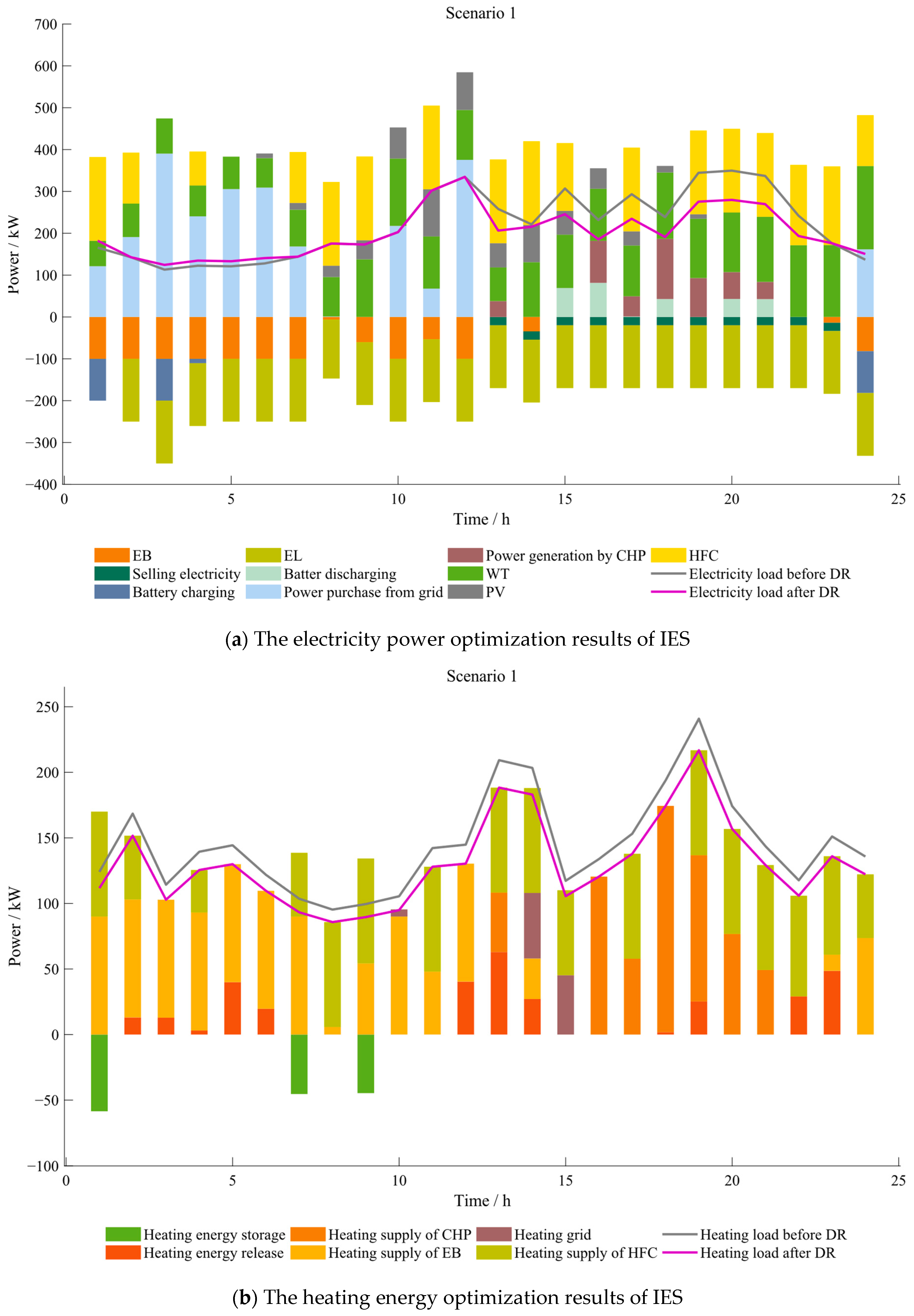
Second, the proposed framework addresses uncertainties in renewable generation and loads through a two-stage DRO approach, which achieves an optimal balance between economic efficiency and operational robustness during scheduling optimization. The integration of demand response mechanisms further enhances system performance by optimizing the distributions of electricity and heating loads, thereby reducing operational costs. The system’s unit regulation costs escalate proportionally with the magnitude of uncertainty. Nevertheless, the model demonstrates adaptive capability across varying scenarios by dynamically adjusting unit power outputs to identify optimal dispatch solutions for cost minimization.

Third, the optimization results obtained under the comprehensive norm constraint demonstrate better economic performance compared to those considering only a single norm constraints. In comparison with conventional uncertainty-handling methodologies SO and RO, the comparative analysis reveals that DRO exhibits enhanced robustness over SO while achieving greater economic efficiency relative to RO, thereby attaining an optimal balance between these two critical operational dimensions.

The proposed model is applicable to community-level IES incorporating electricity, heating, and hydrogen. Future research will focus on the deep integration and coordinated optimization of multiple energy forms by constructing a multi-energy flow coupling model encompassing cooling, heating, electricity, and hydrogen. New technological pathways will be developed, such as the scheduling of absorption cooling driven by the waste heat of hydrogen HFC and electricity-based cooling technologies. On this basis, the model will be integrated with carbon market and electricity market mechanisms to quantify the economic and environmental benefits of cooling systems in DR and low-carbon transition scenarios. Additionally, power flow analysis will be incorporated, and models capable of characterizing DR uncertainties will be designed to further enhance system stability and expand the model’s applicability.

References

1. Amuakwa-Mensah, F.; Näsström, E. Role of banking sector performance in renewable energy consumption. Appl. Energy 2022, 306, 118023. [Google Scholar] [CrossRef]
2. Ren, D.; Xiao, J.; Hou, J.; Du, E.; Jin, C.; Liu, Y. Construction and evolution of China’s new power system under dual carbon goal. Power Syst. Technol. 2022, 46, 3831–3839. [Google Scholar]
3. Yang, Z.; Ren, Z.; Li, H.; Sun, Z.; Feng, J.; Xia, W. A multi-stage stochastic dispatching method for electricity-hydrogen integrated energy systems driven by model and data. Appl. Energy 2024, 371, 123668. [Google Scholar] [CrossRef]
4. Li, Y.; Bu, F.; Gao, J.; Li, G. Optimal dispatch of low-carbon integrated energy system considering nuclear heating and carbon trading. J. Clean. Prod. 2022, 378, 134540. [Google Scholar] [CrossRef]
5. Liu, T.; Yang, Z.; Duan, Y.; Hu, S. Techno-economic assessment of hydrogen integrated into electrical/thermal energy storage in PV+ Wind system devoting to high reliability. Energy Convers. Manag. 2022, 268, 116067. [Google Scholar] [CrossRef]
6. Liu, J.; Li, Y.; Ma, Y.; Qin, R.; Meng, X.; Wu, J. Coordinated energy management for integrated energy system incorporating multiple flexibility measures of supply and demand sides: A deep reinforcement learning approach. Energy Convers. Manag. 2023, 297, 117728. [Google Scholar] [CrossRef]
7. Xuan, A.; Shen, X.; Guo, Q.; Sun, H. A conditional value-at-risk based planning model for integrated energy system with energy storage and renewables. Appl. Energy 2021, 294, 116971. [Google Scholar] [CrossRef]
8. Gargari, M.Z.; Hagh, M.T.; Zadeh, S.G. Preventive scheduling of a multi-energy microgrid with mobile energy storage to enhance the resiliency of the system. Energy 2023, 263, 125597. [Google Scholar] [CrossRef]
9. Gao, Y.; Tahir, M.; Siano, P.; Bi, Y.; Hu, S.; Yang, J. Optimization of renewable energy-based integrated energy systems: A three-stage stochastic robust model. Appl. Energy 2025, 377, 124635. [Google Scholar] [CrossRef]
10. Ma, M.; Long, Z.; Liu, X.; Lee, K.Y. Distributionally robust optimization of electric-thermal-hydrogen integrated energy system considering source-load uncertainty. Energy 2025, 316, 134568. [Google Scholar] [CrossRef]
11. Li, Y.; Wang, J.; Zhang, Y.; Han, Y. Day-ahead scheduling strategy for integrated heating and power system with high wind power penetration and integrated demand response: A hybrid stochastic/interval approach. Energy 2022, 253, 124189. [Google Scholar] [CrossRef]
12. Ding, T.; Yang, Q.; Yang, Y.; Li, C.; Bie, Z.; Blaabjerg, F. A data-driven stochastic reactive power optimization considering uncertainties in active distribution networks and decomposition method. IEEE Trans. Smart Grid 2017, 9, 4994–5004. [Google Scholar] [CrossRef]
13. Wu, M.; Yan, R.; Zhang, J.; Fan, J.; Wang, J.; Bai, Z.; He, Y.; Cao, G.; Hu, K. An enhanced stochastic optimization for more flexibility on integrated energy system with flexible loads and a high penetration level of renewables. Renew. Energy 2024, 227, 120502. [Google Scholar] [CrossRef]
14. Arias, N.B.; Tabares, A.; Franco, J.F.; Lavorato, M.; Romero, R. Robust joint expansion planning of electrical distribution systems and EV charging stations. IEEE Trans. Sustain. Energy 2017, 9, 884–894. [Google Scholar] [CrossRef]
15. Chen, T.; Cao, Y.; Qing, X.; Zhang, J.; Sun, Y.; Amaratunga, G.A. Multi-energy microgrid robust energy management with a novel decision-making strategy. Energy 2022, 239, 121840. [Google Scholar] [CrossRef]
16. Mirzaei, M.A.; Nazari-Heris, M.; Mohammadi-Ivatloo, B.; Zare, K.; Marzband, M.; Shafie-Khah, M.; Anvari-Moghaddam, A.; Catalão, J.P.S. Network-constrained joint energy and flexible ramping reserve market clearing of power-and heat-based energy systems: A two-stage hybrid IGDT–stochastic framework. IEEE Syst. J. 2020, 15, 1547–1556. [Google Scholar] [CrossRef]
17. Zhong, Z.; Fan, N.; Wu, L. Multistage Stochastic optimization for mid-term integrated generation and maintenance scheduling of cascaded hydroelectric system with renewable energy uncertainty. Eur. J. Oper. Res. 2024, 318, 179–199. [Google Scholar] [CrossRef]
18. Bagheri, F.; Dagdougui, H.; Gendreau, M. Stochastic optimization and scenario generation for peak load shaving in Smart District microgrid: Sizing and operation. Energy Build. 2022, 275, 112426. [Google Scholar] [CrossRef]
19. Wang, Z.; Ding, T.; Jia, W.; Huang, C.; Mu, C.; Qu, M.; Shahidehpour, M.; Yang, Y.; Blaabjerg, F.; Li, L.; et al. Multi-stage stochastic programming for resilient integrated electricity and natural gas distribution systems against typhoon natural disaster attacks. Renew. Sustain. Energy Rev. 2022, 159, 111784. [Google Scholar] [CrossRef]
20. Ning, C.; You, F. Data-driven stochastic robust optimization: General computational framework and algorithm leveraging machine learning for optimization under uncertainty in the big data era. Comput. Chem. Eng. 2018, 111, 115–133. [Google Scholar] [CrossRef]
21. Sahebi, A.; Jadid, S. A robust model of local energy market under a security constraint-based approach for distribution system operator and multi-energy microgrids. Electr. Power Syst. Res. 2023, 217, 109164. [Google Scholar] [CrossRef]
22. Fang, F.; Yu, S.; Xin, X. Data-driven-based stochastic robust optimization for a virtual power plant with multiple uncertainties. IEEE Trans. Power Syst. 2021, 37, 456–466. [Google Scholar] [CrossRef]
23. Wang, J.; Xu, X.; Li, H.; Chen, H. Two-stage robust optimization of thermal-ESS units scheduling under wind uncertainty. Energy Rep. 2022, 8, 1147–1155. [Google Scholar] [CrossRef]
24. Yang, J.; Su, C. Robust optimization of microgrid based on renewable distributed power generation and load demand uncertainty. Energy 2021, 223, 120043. [Google Scholar] [CrossRef]
25. Zhang, R.; Chen, Y.; Li, Z.; Jiang, T.; Li, X. Two-stage robust operation of electricity-gas-heat integrated multi-energy microgrids considering heterogeneous uncertainties. Appl. Energy 2024, 371, 123690. [Google Scholar] [CrossRef]
26. Zhu, L.; Wang, J.; Tang, L.; Liu, S.; Huang, C. Robust stochastic optimal dispatching of integrated energy systems considering refined power-to-gas model. Power Syst. Technol. 2019, 43, 116–126. [Google Scholar]
27. He, C.; Zhang, X.; Liu, T.; Wu, L. Distributionally robust scheduling of integrated gas-electricity systems with demand response. IEEE Trans. Power Syst. 2019, 34, 3791–3803. [Google Scholar] [CrossRef]
28. Son, Y.G.; Kim, S.Y. Optimal planning and operation of integrated energy systems in South Korea: Introducing a Novel ambiguity set based distributionally robust optimization. Energy 2024, 307, 132503. [Google Scholar] [CrossRef]
29. Jin, X.; Liu, B.; Liao, S.; Cheng, C.; Zhang, Y.; Zhao, Z.; Lu, J. Wasserstein metric-based two-stage distributionally robust optimization model for optimal daily peak shaving dispatch of cascade hydroplants under renewable energy uncertainties. Energy 2022, 260, 125107. [Google Scholar] [CrossRef]
30. Shui, Y.; Liu, J.; Gao, H.; Huang, S.; Jiang, Z. A distributionally robust coordinated dispatch model for integrated electricity and heating systems considering uncertainty of wind power. Proc. CSEE 2018, 38, 7235–7247. [Google Scholar]
31. Monemi Bidgoli, M. Optimal Energy Management of Water-Energy Nexus in Multi-Carrier Systems Integrated with Renewable Sources. Power Control Data Process. Syst. 2024, 1. [Google Scholar] [CrossRef]
32. Karimi, H.; Hasanzadeh, S.; Saboori, H. Cooperative scheduling and trading in sustainable water-integrated and networked energy systems incorporating power-to-gas. Sustain. Cities Soc. 2024, 101, 105052. [Google Scholar] [CrossRef]
33. Masoudi, M.R.; Haghighi, M.; Rahimipour Behbahani, M. Optimal Operation of Solar Energy System integrated with Energy Storage Systems. Power Control Data Process. Syst. 2024, 1. [Google Scholar] [CrossRef]
34. Haghighi, M.; Masoudi, M.R.; Rahimipour Behbahani, M. Smart Homes Energy Management System Integrated with Renewable Energy Sources and Demand Response Programs. Power Control Data Process. Syst. 2025, 2. [Google Scholar] [CrossRef]
35. Chen, L.; Wu, J.; Wu, F.; Tang, H.; Li, C.; Xiong, Y. Energy flow optimization method for multi-energy system oriented to combined cooling, heating and power. Energy 2020, 211, 118536. [Google Scholar]
36. Guo, Z.; Wang, J.; Dong, F.; Xu, H. Multi-objective optimization of multi-energy complementary system based on cascade utilization of heat storage. Energy Convers. Manag. 2024, 299, 117864. [Google Scholar] [CrossRef]
37. Ma, L.; Xie, L.; Ye, J.; Bian, Y. Two-stage dispatching strategy for park-level integrated energy systems based on a master-slave-cooperative hybrid game model. Renew. Energy 2024, 232, 120971. [Google Scholar] [CrossRef]
38. Liu, R.; Li, Z.; Yang, X.; Sun, G.; Li, L. Optimal dispatch of community integrated energy system considering user-side flexible load. Acta Energiae Solaris Sin. 2019, 40, 2842–2850. [Google Scholar]
39. Li, H.; Lin, L.; Zhao, J. Low carbon economic scheduling of electricity-gas-heat integrated energy system based on demand-side user response analysis. Taiyangneng Xuebao/Acta Energiae Solaris Sin. 2023, 44, 97–105. [Google Scholar]
40. Zhao, C.; Guan, Y. Data-driven stochastic unit commitment for integrating wind generation. IEEE Trans. Power Syst. 2015, 31, 2587–2596. [Google Scholar] [CrossRef]
Figure 1. IES structure diagram.
Mathematics 13 01439 g001
Figure 2. Joint scenario generation flowchart.
Mathematics 13 01439 g002
Figure 3. Solution flowchart.
Mathematics 13 01439 g003
Figure 4. The joint scenario diagram of PV, WT, and loads output generated using MC and the K-means clustering algorithm.
Mathematics 13 01439 g004aMathematics 13 01439 g004b
Figure 5. The joint scenario diagram of PV, WT, and loads output generated using LHS and the K-means clustering algorithm.
Mathematics 13 01439 g005aMathematics 13 01439 g005b
Figure 6. The optimization results of electricity and heating energy for IES.
Mathematics 13 01439 g006
Figure 7. Optimization results of each scheme after electricity and heating energy participate in DR.
Mathematics 13 01439 g007aMathematics 13 01439 g007b
Figure 8. Average Voltage Fluctuation.
Mathematics 13 01439 g008
Figure 9. Average Total Harmonic Distortion.
Mathematics 13 01439 g009
Figure 10. The electricity and heating optimization results of the IES under the second dataset.
Mathematics 13 01439 g010