Spatial Modeling of Auto Insurance Loss Metrics to Uncover Impact of COVID-19 Pandemic

Abstract

This study addresses key challenges in auto insurance territory risk analysis by examining the complexities of spatial loss data and the evolving landscape of territorial risks before and during the COVID-19 pandemic. Traditional approaches, such as spatial clustering, are commonly used for territory risk assessment but offer limited predictive capabilities, constraining their effectiveness in forecasting future losses, an essential component of insurance pricing. To overcome this limitation, we propose an advanced predictive modeling framework that integrates spatial loss patterns while accounting for the pandemic’s impact. Our Bayesian-based spatial model captures stochastic spatial autocorrelations among territory rating units and their neighboring regions. This approach enables more robust pattern recognition through predictive modeling. By applying this approach to regulatory auto insurance loss datasets, we analyze industry-level trends in claim frequency, loss severity, loss cost, and insurance loading. The results reveal significant shifts in spatial loss patterns before and during the pandemic, highlighting the dynamic interplay between regional risk factors and external disruptions. These insights provide valuable guidance for insurers and regulators, facilitating more informed decision-making in risk classification, pricing adjustments, and policy interventions in response to evolving spatial and economic conditions.

1. Introduction

From 2020 to 2022, during the peak of the COVID-19 pandemic, governments worldwide implemented travel restrictions, lockdowns, and social distancing measures to limit virus transmission. As COVID-19 transitioned into an endemic phase, restrictions eased; however, the pandemic’s prolonged effects continue to shape finance, the economy, and daily life. This extended period of lockdowns has had lasting social and economic consequences, prompting significant research into its wide-ranging impacts across sectors, including healthcare [1], education [2], financial markets [3], mental health [4], and tourism [5]. Researchers have sought to understand the systemic transformations triggered by the pandemic, underscoring the importance of studying its effects on societal structures. For example, Ref. [6] examined COVID-19’s effects on Ghana’s insurance industry, employing a comparative methodology to identify parallels with previous pandemics. However, the global response to COVID-19—characterized by its unprecedented scale and the absence of clear geographical or temporal boundaries—has introduced new challenges for insurers, particularly in risk diversification. Unlike previous pandemics or natural disasters, COVID-19 represents a unique global event with few historical precedents, necessitating a focused study of its impact on the auto insurance sector and the broader socio-economic landscape.

In auto insurance rate regulation, the analysis and design of territories present ongoing challenges, particularly due to spatial contiguity requirements. To address these complexities, both traditional clustering methods, such as K-means and fuzzy clustering [7,8,9], and advanced spatial clustering techniques [10,11] have been employed. These methods help create homogeneous groups of spatial risk exposures, enabling the identification of spatial patterns and supporting actuarial fairness in insurance premiums. However, clustering approaches are inherently unsupervised and lack predictive capabilities, limiting their effectiveness in forecasting future losses based on historical data. This limitation highlights the need for predictive models that enhance spatial loss analysis. Accordingly, this study shifts the focus of territory risk analysis from clustering to predictive modeling, aiming to uncover spatial patterns and forecast future territory risks based on key spatial rating units. Prior research has explored spatial patterns in insurance losses [9,12,13], affirming the value of spatial clustering as a complementary approach to predictive modeling. This study extends these efforts by investigating potential shifts in territory risk patterns before and during the COVID-19 pandemic. It aims to identify underlying spatial trends and assess the pandemic’s impact on auto insurance risk. Additionally, it advances the application of spatial data science techniques in insurance pricing, enhancing our ability to analyze and manage territory risks.

To assess the impact of COVID-19, loss data can be analyzed by incorporating time as a covariate or by associating it with spatial locations in the predictive models. These factors can be treated as external variables influencing loss patterns. Model-based approaches offer significant advantages for examining the effects of such external factors. While previous studies have explored the broader economic and financial consequences of COVID-19 on the insurance industry [6,14,15,16], there remains a gap in understanding how the pandemic has influenced spatial patterns of insurance losses and premiums. Given the critical role of geographic location in auto insurance pricing, a detailed analysis of spatial variations in loss and premium data is essential for understanding the pandemic’s effects. This study aims to fill this gap by providing insights that can inform future global health crisis preparedness and improve industry-wide auto insurance rate regulation.

To explore the impact of COVID-19 on auto insurance loss metrics, this paper introduces an innovative approach leveraging spatial models for feature extraction from spatial loss data. Key loss metrics, such as loss cost, are analyzed using spatial models to extract informative parameters that reveal temporal shifts in loss patterns. The spatial models [17,18] used in this study provide a sophisticated statistical framework, incorporating both fixed and random effects within basic rating units, Forward Sortation Areas (FSAs). Grounded in a Bayesian statistical paradigm and inspired by Gaussian mixture random field models, this approach characterizes the stochastic behavior of spatial autocorrelations among FSAs and their neighboring regions using a Gaussian Markov random field. Implemented through Generalized Linear Mixed Models, this additive structure effectively captures both fixed and random spatial effects.

The remainder of this paper is structured as follows: Section 2 reviews existing research on the effects of the COVID-19 pandemic. Section 3 details the spatial models and their application to insurance loss data. Section 4 presents the findings of the analysis. Finally, Section 5 concludes the study and outlines directions for future research.

2. Related Work

In this section, we review key research on the broader economic impact of the COVID-19 pandemic on the insurance industry. The pandemic disrupted both supply and demand in insurance markets, prompting critical responses from insurers and regulators. For example, Ref. [19] provides an extensive overview of the risks posed by COVID-19 and the regulatory measures implemented in response. A surge in claims for life, medical, business interruption, and event cancellation insurance created significant challenges. However, the primary concern for insurers and regulators was financial market instability and the resulting global economic downturn. Ref. [20] supports this perspective, emphasizing that poor investment performance posed a greater risk to insurers than the increase in claims. Both [19,20] discuss how the pandemic strained healthcare systems, leading to delays in non-urgent medical treatments. These delays, in turn, mitigated the immediate impact on life and medical insurance claims. Additionally, the decline in auto insurance claims during lockdowns partially offset the increased losses in life insurance, reflecting an unexpected shift in risk exposure across different insurance lines.

Regulatory interventions during the pandemic aimed to preserve capital while ensuring insurers remained financially stable to meet future obligations [19]. Transparency in insurer responses was critical in maintaining public trust and preventing adverse selection [20]. These studies highlight the necessity of proactive regulatory strategies that balance financial stability, clear communication, and consumer protection. Further regulatory discussions are presented in [21], which examines the National Association of Insurance Commissioners (NAIC) response to the pandemic, particularly regarding catastrophic risk management and health insurance policy changes in a post-pandemic environment. Similarly, Ref. [22] investigates the operational impact of COVID-19 on insurance businesses in the Gulf region, focusing on conduct-of-business regulations. The study highlights how the insurance sector’s shift toward business survival during the crisis may have led to a reduced emphasis on ensuring fair treatment of policyholders.

The COVID-19 pandemic significantly influenced auto insurance pricing, as insurers adjusted loss ratios to maintain actuarial fairness amid shifting driving behaviors. Lockdowns, remote work policies, and social distancing led to a substantial decline in vehicle usage, initially reducing auto insurance claims. However, with the pandemic persisting longer than anticipated, its long-term effects on auto insurance remain uncertain due to complex behavioral and economic factors. Ref. [23] projected changes in U.S. auto insurance by modeling various scenarios based on two key parameters: duration and extent of economic contraction and attitudes and behavioral adaptations. Their study estimated combined ratios of total losses and expenses to earned premiums, providing industry forecasts over an 18-month period. While this scenario-based approach facilitated accessibility, it relied on simplifying assumptions that may not fully capture the evolving nature of driver behavior during the COVID-19 pandemic. Recognizing this limitation, Ref. [24] advocated for a more quantitative approach to assess behavioral shifts in driving patterns. Their study highlighted that government restrictions, hybrid work models, and decreased public transportation use led to significant reductions in road traffic volume and pedestrian movement. However, the study also noted that urban centers experienced a rise in speeding, street racing, and aggressive driving, complicating risk assessment. These findings emphasize that determining the long-term impact of COVID-19 on auto insurance remains challenging, as existing research often simplifies human behavioral responses by relying on subjective assumptions.

Our work advances the literature on auto insurance rate-making by integrating regulatory datasets with predictive spatial modeling, explicitly accounting for spatial autocorrelation in insurance loss analysis. This approach enhances the understanding of spatial loss patterns, offering a more comprehensive perspective than studies that rely solely on individual insurers’ data. By leveraging spatial dependencies, our methodology improves territorial risk assessments, leading to more accurate and equitable premium-setting practices. Furthermore, we extend existing research by examining the impact of COVID-19 on auto insurance pricing and regulation through a spatial lens. The pandemic has reshaped driving behaviors, claim frequencies, and regulatory responses, yet its spatial implications remain underexplored. By applying spatial data science techniques to this emerging challenge, our study contributes to the development of more adaptive and resilient rate-making frameworks that account for dynamic risk factors across different regions.

3. Materials and Methods

3.1. Data and Key Insurance Loss Metrics

The data used in this study are sourced from GISA (https://www.gisa.ca (accessed on 1 January 2025)). This regulatory dataset includes a range of key loss metrics essential for analyzing auto insurance trends in Ontario, Canada. It consists of data information collected from all auto insurance providers in Ontario and includes claim counts, claim amounts, premiums, and risk exposures. Focusing on Forward Sortation Areas (FSAs) over six-month intervals, we derive essential loss indicators such as claim frequency, claim severity, loss cost, and insurance loading. To detect shifts in patterns before and during the COVID-19 pandemic, we examine loss data from 2017 to 2022. The loss data from 2017-1 to 2019-2 are defined as pre-pandemic (before the pandemic), while data from 2020 to 1 to 2022-2 are considered pandemic-period (during the pandemic) data. Our methodology aggregates observations within each FSA, calculating variables such as total claim counts, total vehicle counts, total claim amounts, and total premiums. We further calculate the loss metrics based on the following definitions:

• Claim frequency by FSA is defined as the ratio of total claim counts to total vehicle counts, giving insight into the frequency of claims in specific FSAs.
• Claim severity by FSA is calculated as the total claim amount divided by total claim counts, indicating the average claim size in specific FSAs. In actuarial terms, this represents the average cost to settle a claim within a region, which is a key component for pricing and risk assessment.
• Loss cost by FSA combines claim frequency and severity by multiplying them, offering a comprehensive measure of the financial impact of claims within each FSA. Specifically, it represents the theoretical premium for each exposure.
• Insurance loading is determined by the ratio of premium to loss cost, reflecting the proportion of premiums directed towards covering losses and providing insight into each FSA’s risk profile in relation to insurance pricing and risk management.

For data mapping, we use FSA boundary data from Statistics Canada (https://www.statcan.gc.ca/en/start (accessed on 1 January 2024.)), employing shapefiles to delineate Ontario’s FSA regions. These digital boundaries allow us to visualize loss metric patterns and identify clusters, trends, and spatial autocorrelations. In our spatial modeling, we incorporate the latitude and longitude of the centroid of each FSA as covariates, enhancing the model’s capacity to capture spatial loss patterns and better understand the distribution of risk across the region that we investigate. We also incorporate the estimated COVID-19 cases within each FSA as a covariate in the spatial models. The data, originally aggregated by health units in Ontario, need to be redistributed across the FSAs within each health unit. To achieve this redistribution, we assume that COVID-19 cases are uniformly distributed within each health unit in Ontario.

3.2. Local Moran’s I Statistic

Local Moran’s I statistic is a measure used in spatial statistics to evaluate the stochastic spatial autocorrelation of a variable across different locations. Stochastic spatial autocorrelation (referred to as spatial autocorrelation hereafter) refers to the spatial dependencies that exist between the values of a variable in one FSA and its neighboring FSAs, where the strength and nature of these dependencies are modeled as random processes. In this study, we use Local Moran’s I to capture the dependence structure of the specified loss metrics, helping to identify whether there is clustering, dispersion, or randomness in their spatial distribution. Local Moran’s I reveals how spatial loss metrics relate to those in neighboring areas. To calculate Local Moran’s I statistic, we first compute the spatial lag of the loss metric of interest, $x_i$. The spatial lag for $x_i$ is the weighted average of the loss metric values in the neighboring units of i, determined as follows:

$$\begin{array}{c}\hfill l_i=\sum _{j=1}^n{w}_{ij}·x_j,\end{array}$$

(1)

where n is the total number of spatial units (e.g., FSA in this work), $x_i$ is the value of the loss metric of interest at spatial unit i, and $w_{ij}$ is the spatial weight between spatial units i and j. This weight reflects the spatial relationship between the units and can be binary (indicating adjacency) or distance-based (indicating proximity). In the context of Local Moran’s I applied to insurance loss metrics, the spatial lag helps in identifying clusters of similar loss metrics (high–high or low–low) or spatial outliers (high–low or low–high) by considering the loss metric at a location and comparing it to the weighted average of values at neighboring locations. This is carried out using the following definition of Local Moran’s I. For each spatial unit i, Local Moran’s I is calculated as:

$$\begin{array}{c}\hfill I_i={\displaystyle \frac{(x_i-\overline{x})(l_i-\overline{l})}{{\sigma }^2}},\end{array}$$

(2)

where $\overline{x}$ is the mean of the given loss metrics across all spatial units, $\overline{l}$ is the mean of the spatial lag values across all spatial units and ${\sigma }^2$ is the variance of the loss metrics across all spatial units. In this work, loss metric $x_i$ includes relative claim frequency, claim severity, loss cost, and loading. However, we only report the results using insurance loading to illustrate our important findings.

Note that Local Moran’s I provides information about the degree of spatial association between a specific location and its neighboring locations. Positive values indicate spatial clustering. Negative values indicate spatial outliers, which implies inconsistency of spatial patterns within the neighborhood. Values close to zero suggest spatial randomness. By mapping Local Moran’s I values over accident years, we can visualize the temporal evolution of spatial correlation patterns within a given region, revealing key insights and trends. These findings will be detailed in the Results section.

3.3. Spatial Models

Given that the results from the previous section using Local Moran’s I reveal significant spatial clustering in the loss metrics, it is essential to incorporate spatial structure into the modeling framework. In this section, we focus on the modeling problems of various loss metrics. These metrics can provide crucial insights to auto insurance companies and regulators, particularly in rate regulation. However, selecting an appropriate statistical model to address spatial autocorrelation has remained challenging in spatial data science. In this work, we used both the Besag spatial model and the Besag–York–Mollie (BYM) model to address potential structured and unstructured spatial dependence in the loss data. The Besag model, also known as the Intrinsic Conditional Autoregressive (ICAR) model, is a special case of the Conditional Autoregressive (CAR) family that incorporates spatially structured random effects to account for spatial autocorrelation. Although the general CAR model provides flexibility by including a spatial dependence parameter $\rho$, we adopt the ICAR formulation, obtained by fixing $\rho =1$, for both theoretical and practical reasons. The ICAR model assumes a strong spatial correlation among adjacent areas, which is appropriate given the spatial structure in our data. The BYM model extends this by including an additional unstructured random effect to capture region-specific variation. This approach makes the analysis robust in handling spatial dependencies. To further explain how spatial autocorrelation is captured by a spatial model, we assume that A = $\{1,2,3,\cdots ,n\}$ is a set that contains n different region IDs (i.e., FSA in this work). This set A includes the region i and its surrounding neighbor of i determined by the contiguity method. In this work, each region is represented by an FSA. We also introduce the relation that $i\in A$ and $-i\in A\setminus \left\{i\right\}$ when region i is contained in A, and i is excluded from the set A. The notation $i\sim j$ represents that region j is a neighbor of the region i. $\mathcal{N}\left(i\right)$ is a set containing all neighbors of region i. The spatial autocorrelation between regions i and j, where $j\in \mathcal{N}\left(i\right)$, denoted by ${\eta }_i|{\eta }_{-i}$, or ${\eta }_i|{\eta }_j$, is assumed to be random, and its effect is considered to be normally distributed.

Spatial autocorrelation and spatially structured latent effects are related concepts within spatial statistics, but they capture distinct aspects of spatial dependencies. Spatial autocorrelation refers to the statistical interdependence between observations at different spatial locations, indicating that neighboring locations are more likely to exhibit similar values than those at greater distances. However, spatial autocorrelation can be positive, where neighboring regions have similar values, or negative, where neighboring regions have dissimilar values. Common indices such as Moran’s I or Geary’s C [25] are employed to quantify the extent and strength of spatial clustering or dispersion within a dataset, providing insights into the spatial patterns inherent in the data. On the other hand, spatially structured latent effects are unobservable variables introduced in spatial models, such as Besag’s CAR model, to explicitly account for spatial dependencies. While spatial autocorrelation focuses on observed statistical relationships, spatially structured latent effects are introduced into models to represent the underlying spatial dependencies that contribute to the observed autocorrelation. In essence, spatial autocorrelation is a descriptive measure of observed spatial relationships, whereas spatially structured latent effects are a modeling tool to explicitly account for and incorporate spatial dependencies within the statistical framework. In this study, we employ both approaches for analyzing the spatial patterns of auto insurance loss metrics. From an insurance rate regulation perspective, descriptive measures of spatial dependence provide insurance companies and regulators with an intuitive tool for analyzing spatial patterns. Additionally, incorporating spatial structure enhances the robustness and reliability of the statistical approaches used for quantifying these patterns.

From modeling and parameter estimation perspectives, the Bayesian approach offers flexibility and robustness that are essential for capturing complex spatial dependencies and latent structures. However, traditional Bayesian inference methods such as Markov Chain Monte Carlo (MCMC) can be computationally intensive and slow to converge. To address this challenge, we chose to use Integrated Nested Laplace Approximation (INLA), which provides a fast and accurate deterministic alternative to the MCMC approach. INLA is specifically designed for latent Gaussian models and is highly efficient in approximating posterior distributions without the need for extensive sampling. Moreover, Besag and BYM models also benefit from computational efficiency due to their sparse precision matrix and are well supported in modern Bayesian frameworks such as INLA employed in this study. This makes it especially suitable for high-dimensional spatial models.

3.3.1. Poisson–Besag Spatial Model for Claim Frequencies

The Besag model, being relatively simple and widely used, serves as a natural starting point for our exploration of spatial models. The Poisson–Besag spatial model is often applied in the context of areal data, where the Poisson distribution is assumed to capture the randomness associated with the spatial count data. When it is applied to spatial loss data, the model incorporates both a Poisson distribution for the observed claim counts and a spatially correlated random effect term. The Poisson–Besag spatial model is defined as follows: Let $Y_i$ be the observed claim count at location i, where $i=1,2,\dots ,n$. The observed counts are assumed to follow a Poisson distribution:

$$\begin{array}{c}\hfill Y_i\sim \mathrm{Poisson}\left({\lambda }_i\right),\end{array}$$

(3)

where ${\lambda }_i$ is the expected mean claim count at location i. The expected mean ${\lambda }_i$ is then modeled as a combination of an underlying intensity term ${\mu }_i$ and a spatially correlated random effect term ${\eta }_i$:

$$\begin{array}{c}\hfill {\lambda }_i={\mu }_i\exp \left({\eta }_i\right),\end{array}$$

(4)

where the underlying intensity term ${\mu }_i$ is proportionate to risk exposure, which is the number of vehicles, denoted by $E_i$. That is,

$$\begin{array}{c}\hfill {\mu }_i=E_i\exp \left({\beta }_0\right),\end{array}$$

(5)

where $\exp \left({\beta }_0\right)$ is the baseline claim frequency and ${\beta }_0$ represents the fixed effect in the following log-link function for Poisson regression:

$$\begin{array}{c}\hfill log\left({\lambda }_i\right)=log\left(E_i\right)+{\beta }_0+{\eta }_i.\end{array}$$

(6)

The spatially structured latent variable ${\eta }_i$ follows a Conditional Autoregressive (CAR) process. Let $\mathcal{N}\left(i\right)$ denote the set of neighbors for location i, and $w_{ij}$ be the spatial weight between locations i and j. The spatial structure is then modeled as:

$${\eta }_i|{\eta }_{-i}\sim \mathcal{N}\left({\displaystyle \frac{{\sum }_{j\in \mathcal{N}\left(i\right)}{w}_{ij}{\eta }_j}{{\sum }_{j\in \mathcal{N}\left(i\right)}{w}_{ij}}},{\displaystyle \frac{\tau }{{\sum }_{j\in \mathcal{N}\left(i\right)}{w}_{ij}}}\right),i=1,2,\dots ,n.$$

(7)

Often, the spatial weights are taken as binary adjacency: $w_{ij}$ = 1 if i and j are neighbors, 0 otherwise. Based on this, the joint spatially correlated random effect $\mathsf{\eta }$ = $({\eta }_1,{\eta }_2,\dots ,{\eta }_n)$ is modeled as a Gaussian Markov random field (GMRF):

$$\begin{array}{c}\hfill \mathsf{\eta }\sim \mathrm{GMRF}(\mathbf{0},\tau {\left(Q\right)}^{-1}),\end{array}$$

(8)

where $\tau$ is the precision parameter that controls the variance and Q is the precision matrix. The precision matrix Q encodes the spatial correlation structure. It is often constructed based on the neighborhood structure of the spatial locations. For a set of neighboring locations $\mathcal{N}\left(i\right)$, the precision matrix element $Q_{ij}$ is defined as:

$$\begin{array}{c}\hfill Q_{ij}=\left\{\begin{array}{cc}\left|\mathcal{N}\left(i\right)\right|\hfill & \mathrm{if}i=j,\hfill \\ -w_{ij}\hfill & \mathrm{if}i\ne j\mathrm{and}j\in \mathcal{N}\left(i\right),\hfill \\ 0\hfill & \mathrm{otherwise}.\hfill \end{array}\right.\end{array}$$

(9)

Assuming the spatially autocorrelated random effect is a Gaussian Markov random field that facilitates its Bayesian analysis, the prior distribution for the precision parameter $\tau$ is often chosen as a Gamma distribution: $\tau \sim \mathrm{Gamma}(a,b),$ where a and b are shape and rate parameters, respectively. The choice of a Gamma distribution for the prior distribution of the precision parameter $\tau$ in the Poisson–Besag spatial model is a common practice in Bayesian statistics. The Gamma distribution is a flexible family of distributions that can take on a variety of shapes, making it suitable for modeling positive continuous random variables, such as precision parameters. The Gamma distribution is particularly convenient for modeling precision parameters because it is defined on the positive real line, and its shape can be adjusted to accommodate various prior beliefs about the precision. In Bayesian spatial modeling, the Gamma distribution is commonly used as a prior for precision parameters due to its conjugacy in hierarchical models and its flexibility in expressing prior beliefs about precision. This means that when combined with a likelihood, the posterior distribution for $\tau$ is also a Gamma distribution.

To examine the influence of covariates on the response variable in the spatial model, we employ the following complete model and extract the covariate coefficients as key features for analyzing the primary loss metrics:

$$\begin{array}{ccc}\hfill M_0:E\left(log\left({\lambda }_i\right)\right)& =& log\left(E_i\right)+{\beta }_0+{\beta }_1{\mathrm{COVID}\_\mathrm{label}}_i+{\beta }_2{\mathrm{centroid}\_\mathrm{lat}}_i+{\beta }_3{\mathrm{centroid}\_\mathrm{long}}_i\hfill \\ & +& {\beta }_4{\mathrm{year}\_\mathrm{label}}_i+{\beta }_5{\mathrm{vech}\_\mathrm{den}}_i+{\beta }_6{\mathrm{est}\_\mathrm{case}}_i,\hfill \end{array}$$

(10)

where COVID_label indicates whether the data correspond to a COVID year, centroid_lat and centroid_long denoted the latitude and longitude of the centroid of FSA, respectively, year_label is the accident half year and takes value from 1 to 10, vech_den corresponds to the calculated vehicle density, and the est_case represents the estimated number of COVID-19 cases for each FSA. The estimated cases are derived under the assumption that cases are uniformly distributed within each health unit encompassing multiple FSA areas.

To better study the impact on the intensity of Poisson distribution, we consider the following three different models for modeling the claim frequency

$$M_1:E\left(log\left({\lambda }_i\right)\right)=log\left(E_i\right)+{\beta }_0+{\beta }_1{\mathrm{COVID}\_\mathrm{label}}_i+{\beta }_2{\mathrm{centroid}\_\mathrm{lat}}_i$$

(11)

$$\begin{array}{ll}{M}_2:E\left(log\left({\lambda }_i\right)\right)& =log\left(E_i\right)+{\beta }_0+{\beta }_1{\mathrm{COVID}\_\mathrm{label}}_i+{\beta }_2{\mathrm{centroid}\_\mathrm{lat}}_i\\ & +{\beta }_3{\mathrm{year}\_\mathrm{label}}_i\end{array}$$

(12)

$$\begin{array}{ll}{M}_3:E\left(log\left({\lambda }_i\right)\right)& =log\left(E_i\right)+{\beta }_0+{\beta }_1{\mathrm{COVID}\_\mathrm{label}}_i+{\beta }_2{\mathrm{centroid}\_\mathrm{lat}}_i+{\beta }_3{\mathrm{year}\_\mathrm{label}}_i\\ & +{\beta }_4{\mathrm{vech}\_\mathrm{den}}_i+{\beta }_5{\mathrm{estimated}\_\mathrm{case}}_i.\end{array}$$

(13)

Note that for all three models, the included covariates are statistically significant within each model. Longitude was excluded as a covariate due to its insignificance in the model. The $M_1$ model captures the influence of spatial location and the COVID-19 pandemic on the response variable. Building on $M_1$, the $M_2$ model incorporates the time effect by including accident half-year as a covariate. The $M_3$ model further extends $M_2$ by accounting for the impact of vehicle density and COVID-19 case counts within the FSAs.

3.3.2. Poisson Besag–York–Mollié Model

The Poisson Besag–York–Mollié (BYM) model is an extension of the Poisson–Besag spatial model, introducing additional components to account for unstructured variability and overdispersion in the observed counts. In the Poisson BYM model, the expected mean ${\lambda }_i$ is modeled as a combination of terms:

$$\begin{array}{c}\hfill {\lambda }_i={\mu }_i\exp ({\eta }_i+u_i)=E_i\exp ({\beta }_0+{\eta }_i+u_i),\end{array}$$

(14)

where ${\mu }_i$ is the underlying intensity, which is equal to $E_i\exp \left({\beta }_0\right)$, ${\eta }_i$ is the spatially correlated random effect, and $u_i$ is the unstructured random effect. The spatially correlated random effect $\mathsf{\eta }$ is also modeled as a Gaussian Markov random field (GMRF), similar to Equation (8). The unstructured random effect $u_i$ is modeled as an independent and identically distributed (i.i.d.) normal random variable:

$$\begin{array}{c}\hfill u_i\sim \mathcal{N}(0,{\lambda }_u^{-1}),\end{array}$$

(15)

where ${\lambda }_u$ is the precision parameter. The log-link function becomes:

$$\begin{array}{c}\hfill \log \left({\lambda }_i\right)=\log \left(E_i\right)+{\beta }_0+{\eta }_i+u_i.\end{array}$$

(16)

The prior distributions for the precision parameters are chosen as Gamma distributions: $\tau \sim \mathrm{Gamma}(a_{\tau },b_{\tau })$ and ${\lambda }_u\sim \mathrm{Gamma}(a_u,b_u)$. In the Poisson BYM model, the choice of a Gamma distribution for precision parameters ($\tau$ and ${\lambda }_u$) is motivated by both mathematical convenience and statistical considerations, which is similar to the Poisson–Besag model. The Gamma distribution provides flexibility in capturing a range of prior beliefs about precision, as it can take on various shapes. This flexibility is essential when modeling uncertainty in the spatial autocorrelation structure.

3.3.3. Other Besag Spatial Models

For modeling claim frequency, a Poisson-based spatial model may be ideal due to the discrete nature of claim frequency. However, when modeling other loss metrics, including claim severity and insurance premium loadings, a Gaussian or other continuous probability distribution-based spatial model may be more appropriate to capture the natural variation in the underlying response variable. In contrast to Poisson models, Gaussian or other continuous probability distribution models inherently account for random variation through their error structures. As a result, incorporating an additional unstructured random effect is generally unnecessary. Therefore, for the remaining model specifications, we focus exclusively on Besag models.

Let $Y_i$ be the observed data (it can be the empirical premium loading, or claim severity, etc.) at locations $i=1,2,\dots ,n$, and $\eta$ be a spatially structured latent variable. The Gaussain Besag’s spatial model can be described as follows:

$$Y_i|{\eta }_i,{\sigma }^2\sim \mathcal{N}({\eta }_i,{\sigma }^2),i=1,2,\dots ,n.$$

(17)

Here, ${\sigma }^2$ is the variance parameter, representing the amount of unstructured variability in the spatial data. The Gaussian Besag spatial model and the Poisson–Besag spatial model are both widely used in Bayesian spatial statistics. Although the same data used for the Poisson–Besag spatial model can be used to fit the Gaussian Besag spatial model without technical issues, each model has distinct advantages and disadvantages. Comparing the two models can help in selecting the most appropriate approach based on the nature of the data and the objectives of the analysis.

The Gaussian Besag spatial model is advantageous when dealing with continuous data, as it assumes a normal distribution. This makes it suitable for scenarios where measurements or variables can take on a wide range of values. However, the Gaussian model has limitations. It assumes that the data follow a normal distribution, which may not be appropriate for datasets that are heavily skewed or exhibit non-Gaussian characteristics. Furthermore, while the model is relatively robust to outliers, extreme values can still influence parameter estimates, potentially affecting model performance. To address this, alternative continuous distributions such as the Gamma and Log-Normal models are often used for modeling other loss metrics, including loss cost, claim severity, and premium loadings. The specification of the likelihood functions for these distributions follows a similar structure to those employed under Gaussian and Poisson models. In this work, we model claim severity, loss cost, and loadings using various spatial models, each based on different distributional assumptions for the response variable.

4. Results

In this section, we analyze the temporal evolution of spatial patterns in loss metrics including insurance loadings and loss costs using Local Moran’s I to capture spatial autocorrelation. Insurance loadings are used to capture how insurers adjust their pricing in response to significant shifts in insurance losses during the pandemic, while loss costs reflect changes in the underlying cost of providing coverage. By applying Moran’s I statistic, we can assess the spatial structure of risk, identifying whether it exhibits homogeneity or heterogeneity across different regions. Regions with high positive values of Local Moran’s I indicate consistent insurance loadings, suggesting that FSAs within these areas form homogeneous clusters in terms of pricing adjustments. Conversely, low or negative values signify variability in insurance loading, indicating inconsistencies across the region. The primary goal of this illustration is to demonstrate how spatial autocorrelation, as measured by Moran’s I, can be utilized to identify spatial patterns influenced by key factors of interest. This approach highlights not only the geographical patterns of loss metrics but also how they evolve over time, reflecting changes in the underlying insurance loss dynamics. These findings support our further exploration of spatio-temporal models to more accurately capture these underlying changes.

Examining spatial autocorrelation in insurance loading is particularly relevant in the context of COVID-19, which significantly disrupted insurance pricing dynamics. Insurance loading encompasses factors beyond pure premiums (i.e., loss costs), including administrative expenses, profit margins, and market adjustments, all of which were influenced by pandemic-induced shifts in driving behavior, claim frequency, and economic uncertainty. Unlike direct loss metrics such as loss cost, frequency, and severity, loading reflects insurers’ strategic responses to these disruptions across different regions. Investigating its spatial patterns helps identify regional disparities, assess pricing fairness, and refine risk adjustment models by incorporating spatial dependencies. Furthermore, this analysis supports regulatory decision-making by determining whether regional pricing variations align with actual risk differences or reflect market distortions exacerbated by the pandemic. However, to gain deeper insights into the spatial patterns of other relevant loss metrics, we also included results based on loss costs. This allows for a better understanding of the temporal evolution of clustering behavior in territorial risk.

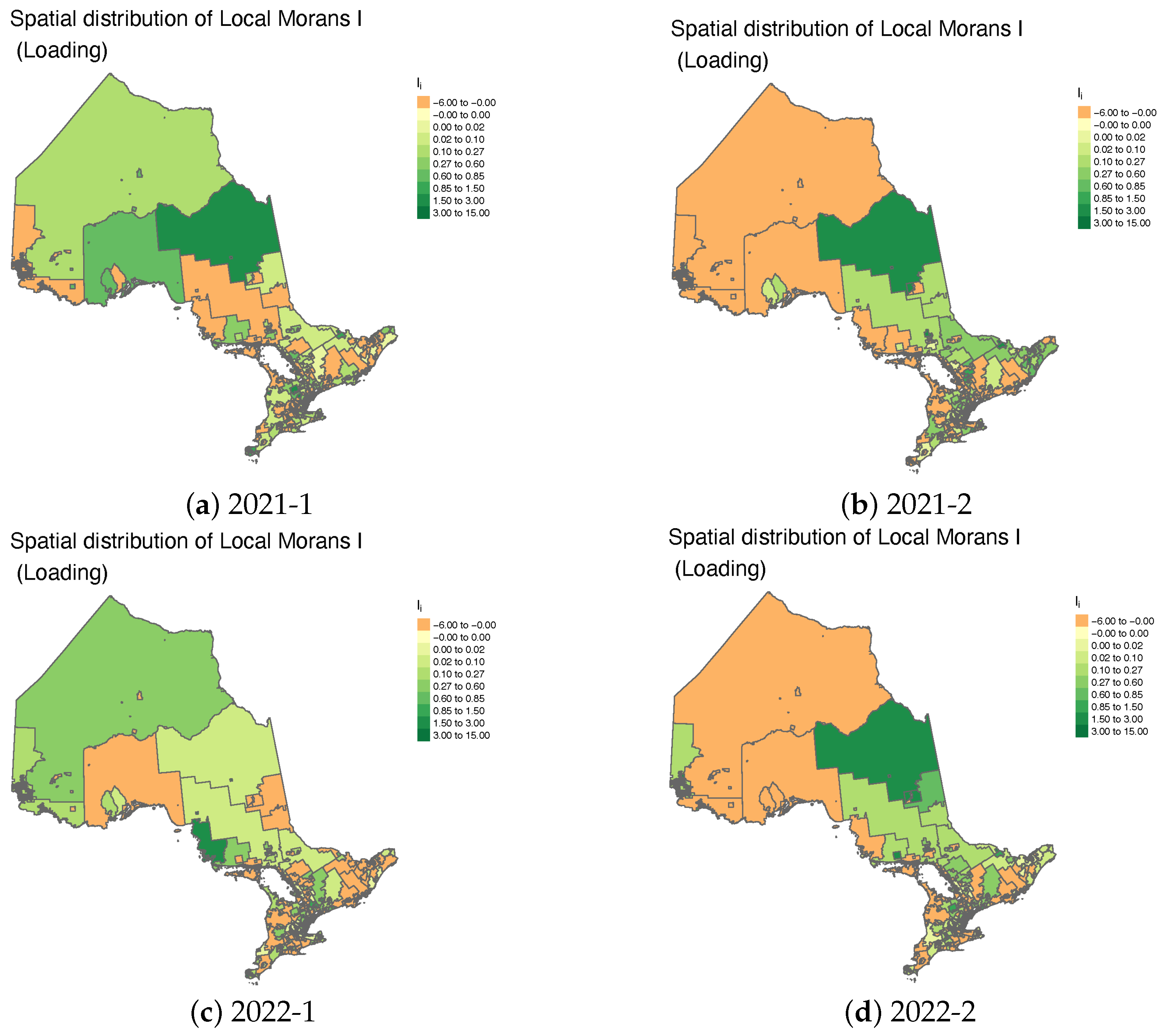
We first present results for the entire province of Ontario before narrowing our focus to southern Ontario, a key economic region. The heat maps in Figure 1 and Figure 2, which depict the spatial distribution of Local Moran’s I, show that spatial autocorrelation in insurance loading remained relatively stable before and at the onset of the COVID-19 pandemic, specifically during 2019-1, 2019-2, and 2020-1. A notable observation is the stronger consistency of insurance loading in northern Ontario, in contrast to the greater heterogeneity observed in southern Ontario during these periods. This spatial inconsistency worsened in 2020-2, coinciding with the implementation of lockdown measures, and has persisted through 2022. Figure 3 and Figure 4 illustrate the temporal evolution of spatial autocorrelation in southern Ontario. A notable prevalence of regions with negatively large Local Moran’s I values is observed, particularly in 2019-1, with this pattern persisting both before and throughout the pandemic. This indicates sustained spatial heterogeneity in insurance loading, suggesting inconsistencies in pricing adjustments across neighboring regions. When insurance loading is used to compute Local Moran’s I, negatively large values indicate strong spatial heterogeneity, where FSAs with high loading are surrounded by those with low loading or vice versa. This pattern reflects pricing discontinuities that may arise from market inefficiencies, regulatory interventions, or localized risk misestimations. Conversely, small or near-zero values suggest weak or no significant spatial autocorrelation, implying that insurance loading is more randomly distributed across regions. In such cases, pricing adjustments are likely driven by individual underwriting decisions rather than broader regional trends. Identifying these spatial patterns is essential for evaluating pricing fairness, regulatory compliance, and the alignment of insurance premiums with actual risk factors.

As discussed earlier, analyzing the temporal evolution of spatial patterns in loss cost is crucial for understanding the dynamics of territorial risk. This is especially important when examining the impact of extraordinary events, such as the COVID-19 pandemic, on insurance costs. Figure 5, Figure 6, Figure 7 and Figure 8 illustrate how spatial autocorrelation patterns in loss cost vary across different accident half years throughout Ontario. Notably, during the pandemic period, the spatial patterns become more heterogeneous, particularly in the southern regions of the province. This spatial variability may be attributed to a significant decline in claim frequency due to lockdown policies, which in turn reduces the dependence of loss costs on neighboring areas.

From an insurance rate regulation perspective, these findings have important implications. They suggest that traditional territorial rating models, which often rely on spatial stability and correlation, may require re-evaluation during periods of systemic disruption. The diminished spatial dependence observed during the pandemic indicates that using historical spatial relationships as a basis for territorial classification could lead to inaccuracies in risk assessment and unfair pricing. As such, regulatory frameworks should consider incorporating dynamic spatial models that account for temporal shifts in risk patterns, especially under conditions of societal or economic stress.

Table 1. Summary of the model output for claim frequency modeling. Poisson–Besag spatial model was used to produce the results.

Covariates	Mean	SD	1st Quantile	2nd Quantile	3rd Quantile
(Intercept)	0.9536	1.4133	−1.8192	0.9535	3.7267
year_label	−0.0125	0.0003	−0.0130	−0.0125	−0.0119
COVID_label	−0.3544	0.0013	−0.3570	−0.3544	−0.3518
est_cases	−0.0002	0.0000	−0.0002	−0.0002	−0.0001
centroid_lat	−0.1053	0.0254	−0.1552	−0.1053	−0.0554
centroid_long	−0.0176	0.0134	−0.0439	−0.0176	0.0086

,

Table 2. Summary of the model output for severity. Gamma Besag’s spatial model was used to model the severity.

Covariates	Mean	SD	1st Quantile	2nd Quantile	3rd Quantile
(Intercept)	2.2138	0.1351	1.9486	2.2138	2.4786
vech_den	−0.0000061	0.0000020	−0.0000101	−0.0000061	−0.0000021
year_labels	0.0038	0.0002	0.0035	0.0038	0.0042
COVID_label	−0.0041	0.0008	−0.0058	−0.0041	−0.0025
est_case	−0.0000132	0.0000019	−0.0000168	−0.0000132	−0.0000096
centroid_lat	0.0004	0.0026	−0.0048	0.0004	0.0055
centroid_long	0.0001	0.0012	−0.0023	0.0001	0.0026

,

Table 3. Summary of the model output for loss cost. Gamma Besag’s spatial model was used to model the loss cost.

Covariates	Mean	SD	1st Quantile	2nd Quantile	3rd Quantile
(Intercept)	2.3481	0.2910	1.7772	2.3481	2.9191
vech_den	0.0000051	0.0000040	−0.0000029	0.0000051	0.0000130
year_label	0.0034	0.0003	0.0028	0.0034	0.0039
COVID_label	−0.0577	0.0013	−0.0601	−0.0577	−0.0552
est_case	−0.0000376	0.0000028	−0.0000432	−0.0000376	−0.0000321
centroid_lat	−0.0130	0.0055	−0.0238	−0.0130	−0.0023
centroid_long	−0.0019	0.0027	−0.0072	−0.0019	0.0034

and

Table 4. Summary of the model output for loading. Gamma Besag’s spatial model was used to model the loading.

Covariates	Mean	SD	1st Quantile	2nd Quantile	3rd Quantile
(Intercept)	−1.5301	1.2669	−4.0182	−1.5293	0.9539
vech_den	0.0000187	0.0000195	−0.0000195	0.0000187	0.0000569
year_label	−0.0059	0.0019	−0.0096	−0.0059	−0.0022
COVID_label	0.4379	0.0082	0.4219	0.4379	0.4540
est_case	0.0002490	0.0000186	0.0002127	0.0002490	0.0002855
centroid_lat	0.0599	0.0246	0.0116	0.0598	0.1083
centroid_long	0.0092	0.0116	−0.0135	0.0092	0.0319

summarize the model output using Besag’s spatial model applied to claim frequency, severity, loss cost, and loading. For each model covariate, the first three quantiles, mean, and standard deviation are reported. Our primary focus is on the sign of each parameter estimate, as it indicates whether a covariate has a positive or negative impact on the response variable.

In Table 1, all parameter estimates for covariates associated with the highest absolute values of COVID_label are negative, suggesting a strong influence of COVID-19 in reducing overall claim frequency. Additionally, spatial location variables also exhibit negative effects on claim frequency, which may indicate a significant territorial shift in risk during the pandemic. However, the impact of COVID_label on claim severity is not as pronounced. While vehicle density and estimated COVID-19 cases contribute to a decrease in severity, spatial location as a risk factor has a positive effect, further reinforcing the notion of shifting territorial risk patterns during the pandemic. As expected, accident year, as a temporal factor, is associated with an increasing trend in severity.

Examining the combined effects of claim frequency and severity, as reflected in loss cost (Table 3), we find that COVID_label, est_case, and centroid_lat, all have negative effects on loss cost, whereas vehicle density within an FSA and accident year contribute to an increase. Notably, when analyzing the impact on insurance loading, all covariates except accident year exhibit a positive influence, suggesting that insurers adjusted their pricing strategies by incorporating spatial and pandemic-related factors into their premium structures.

To determine the most suitable spatial model for each loss metric, we fit the data to various models (see Equation (11)) while assuming different distributional forms for the response variable. Model performance is evaluated using multiple goodness-of-fit metrics, including Mean Squared Error (MSE), Root Mean Squared Error (RMSE), Deviance Information Criterion (DIC), and Watanabe–Akaike Information Criterion (WAIC). The results, summarized in

Table 5. M1: Model using latitude and COVID label as predictors. M2: Enhance the M1 by incorporating year labels as predictors. M3: Enhance the M2 by incorporating the estimated number of COVID cases as predictors. _Poisson, _Gamma, _Log: Models with select Poisson, Gamma, and Log-Normal distribution for the response, respectively. Mean Square Error (MSE), Root Mean Square Error (RMSE), Deviance Information Criterion (DIC) and Watanabe–Akaike Information Criterion (WAIC) are used to quantify the goodness of the spatial models.

	Model	MSE	RMSE	DIC	WAIC
Claim Frequency	M1_Poisson	0.000053	0.007257	74,638.3	124,809.73
	M2_Poisson	0.000058	0.007637	62,156.54	84,293
	M3_Poisson	0.000053	0.007257	59,799.13	76,356.4
Severity	M1_Gamma	12,070,481	3474.45	91,508.20	92,601.86
	M1_LogNormal	12,508,098	3536.67	91,269.06	91,325.25
	M2_Gamma	11,181,007	3343.80	90,979.71	92,454.85
	M2_LogNormal	11,573,098	3401.93	90,794.83	90,866.52
	M3_Gamma	11,081,120	3328.83	90,923.92	92,351.89
	M3_LogNormal	11,468,396	3386.50	90,739.45	90,823.13
Severity with Log transform	M1_Gamma	12,484,100	3533.28	892.63	934.50
	M1_LogNormal	12,539,582	3541.12	861.39	886.32
	M2_Gamma	11,551,397	3398.73	414.63	473.75
	M2_LogNormal	11,603,306	3406.36	379.25	423.85
	M3_Gamma	11,448,492	3383.56	359.67	425.93
	M3_LogNormal	11,497,201	3390.75	322.76	368.73
Loss Cost	M1_Gamma	82,758.45	287.68	67,878.23	68,686.89
	M1_LogNormal	85,559.94	292.51	67,685.22	67,742.12
	M2_Gamma	82,652.53	287.49	67,868.19	68,688.74
	M2_Log	85,439.72	292.30	67,677.16	67,734.48
	M3_Gamma	78,876.16	280.85	67,656.54	68,620.69
	M3_LogNormal	81,445.28	285.39	67,463.77	67,526.44
Loss Cost with Log transform	M1_Gamma	85,735.09	292.81	1688.88	1816.76
	M1_LogNormal	86,316.14	293.79	1663.02	1705.35
	M2_Gamma	85,613.71	292.59	1680.46	1818.59
	M2_LogNormal	86,208.27	293.61	1655.70	1698.09
	M3_Gamma	81,884.2	286.15	1490.12	1657.11
	M3_LogNormal	82,438.64	287.12	1465.38	1509.55
Loading	M1_Gamma	0.2490	0.4990	6270.11	6278.21
	M1_Log	0.2602	0.5101	6483.96	6518.31
	M2_Gamma	0.2445	0.4944	6175.38	6182.15
	M2_LogNormal	0.2555	0.5055	6404.15	6437.49
	M3_Gamma	0.2346	0.4844	5986.85	5991.05
	M3_LogNormal	0.2457	0.4957	6227.06	6268.07

, indicate that the Gamma distribution, when combined with the M3 model, provides a strong fit for most loss metrics. However, for claim frequency, the Poisson distribution emerges as a more appropriate choice, reflecting the discrete nature of frequency data. Additionally, within claim frequency modeling, the M3 model is preferred due to its consistently lower DIC and WAIC values, suggesting better model parsimony and predictive accuracy. These findings underscore the importance of selecting an appropriate distributional assumption and spatial model structure when modeling different components of insurance risk. By leveraging the Gamma distribution for continuous loss metrics and the Poisson distribution for frequency data, insurers can improve predictive accuracy and enhance the robustness of auto insurance pricing models.

The analysis of covariate effects on loss metrics in the Besag spatial model provides insights into overall trends for the accident years 2018 to 2022. However, the obtained results offer a limited perspective on the direct impact of the COVID-19 pandemic. To address this limitation, we further examine the temporal evolution of estimated loss metrics using spatial models and compare them to empirical estimates. This approach allows us to identify potential structural changes or significant shifts within each time period. To capture these temporal dynamics, we compare the first (Q1), second (Q2), and third (Q3) quantiles of the estimated loss metrics for each half-year accident period across various spatial models. The results, presented in Figure 9, reveal a significant drop in claim frequency during the peak of the COVID-19 pandemic. Claim frequency begins to recover after the second half of 2021, coinciding with the Ontario government’s removal of stay-at-home policies.

In contrast, claim severity exhibits a gradual upward trend over time, suggesting a more moderate and sustained impact. When examining loss cost, which reflects the combined effects of claim frequency and severity, the temporal pattern closely aligns with that of claim frequency. This finding implies that the pandemic’s influence on claim frequency was the dominant driver of changes in loss cost. Furthermore, the observed peak in insurance loading during the pandemic period suggests that insurers adopted a more conservative approach to premium adjustments, likely as a response to heightened uncertainty. This raises potential concerns regarding actuarial fairness in pricing during the pandemic, as higher loading may have disproportionately affected certain policyholders.

We further analyze the role of spatial location in predictive modeling by comparing two scenarios: one where spatial location is included as a covariate and another where it is omitted. This comparison allows us to assess the impact of spatial factors on the estimation of loss metrics. The results are presented in Figure 10 and Figure 11. Additionally, we compare these trends with the pre-pandemic period (i.e., 2017–2019), which serves as a baseline to isolate the effects of the pandemic. This comparison reveals that prior to the pandemic, loss metrics were relatively stable, with no significant upward or downward trends. The disruption caused by the pandemic (2020–2021) is more pronounced in claim frequency, loss cost, and loading, highlighting the distinct impact of COVID-19.

In Figure 10, where spatial locations are excluded, the spatial models primarily capture broad trends or local averages within specific time periods, but they fail to account for finer spatial variations. This limitation is particularly evident in periods where the loss metric patterns exhibit significant fluctuations. In contrast, when spatial location is incorporated into the model (Figure 11), the predicted loss metrics align much more closely with observed values, highlighting the crucial role of spatial information in refining model accuracy.

This finding underscores the importance of incorporating spatial dependencies in auto insurance pricing, as it enhances the ability to capture localized risk variations and improves the predictive performance of loss metrics. Given the inherently geographic nature of insurance risk—where factors such as traffic density, road conditions, and regional economic activity influence claim patterns—spatial modeling provides a more precise and equitable framework for premium adjustments.

5. Conclusions and Future Work

In this study, we analyzed spatial loss patterns in auto insurance before and during the COVID-19 pandemic, applying advanced spatial models to capture and interpret these patterns comprehensively. This approach provides a deeper understanding of how the pandemic influenced auto insurance losses across different regions, underscoring the critical role of spatial risk assessment in insurance pricing and regulation. Our results reveal clear spatial heterogeneity in key loss metrics, with notable reductions observed in urban centers during the pandemic, while some rural and suburban regions exhibited more stable patterns. Such geographic variations are precisely the kind that spatially structured models are designed to capture. Our findings highlight that incorporating spatial dependencies into loss modeling enhances predictive accuracy and facilitates more equitable risk-based pricing strategies.

Despite the growing relevance of spatial data science, its application in auto insurance remains largely underexplored. This study contributes to the field by integrating spatial modeling techniques within the context of insurance rate regulation and insurance pricing, introducing a novel framework for assessing the geographic distribution of risk. Through a rigorous analysis of key loss metrics—including claim frequency, severity, loss cost, and insurance loading—we identify distinct spatial trends and shifts between before and during pandemic periods. These insights are critical for insurers, regulators, and policymakers aiming to refine territorial risk classification and pricing fairness in response to external disruptions. The impact of this research extends beyond COVID-19, providing a robust methodology for analyzing spatial variations in insurance losses under evolving economic and behavioral conditions. By demonstrating the effectiveness of spatial modeling in capturing geographic disparities, this work lays the foundation for more adaptive and resilient insurance pricing frameworks.

To build on these findings, we recommend that the auto insurance industry invest in the development of dynamic, spatially aware pricing systems that integrate real-time geographic and behavioral data. This requires moving beyond static territorial classifications toward adaptive models that account for evolving mobility patterns, infrastructure changes, and socio-economic shifts. Insurers should also collaborate with urban planners and transportation agencies to proactively assess emerging risk landscapes, particularly in the context of climate change, increasing telematics adoption, and autonomous vehicle deployment. By embedding more spatial intelligence into pricing and regulatory frameworks, the industry can better anticipate future disruptions, promote fairness, and support data-driven policy interventions.

Future research will extend this framework to analyze long-term post-pandemic effects and incorporating machine learning techniques for spatial–temporal pattern detection could offer new insights into emerging risk landscapes. As autonomous vehicles and usage-based insurance gain prominence, future studies should also investigate how spatial dependencies interact with these innovations, shaping the next generation of auto insurance risk assessment models.

References

1. Kaye, A.D.; Okeagu, C.N.; Pham, A.D.; Silva, R.A.; Hurley, J.J.; Arron, B.L.; Sarfraz, N.; Lee, H.N.; Ghali, G.E.; Gamble, J.W.; et al. Economic impact of COVID-19 pandemic on healthcare facilities and systems: International perspectives. Best Pract. Res. Clin. Anaesthesiol. 2021, 35, 293–306. [Google Scholar] [CrossRef]
2. Pokhrel, S.; Chhetri, R. A literature review on impact of COVID-19 pandemic on teaching and learning. High. Educ. Future 2021, 8, 133–141. [Google Scholar] [CrossRef]
3. Ashraf, B.N. Economic impact of government interventions during the COVID-19 pandemic: International evidence from financial markets. J. Behav. Exp. Financ. 2020, 27, 100371. [Google Scholar] [CrossRef]
4. Xiong, J.; Lipsitz, O.; Nasri, F.; Lui, L.M.; Gill, H.; Phan, L.; Chen-Li, D.; Iacobucci, M.; Ho, R.; Majeed, A.; et al. Impact of COVID-19 pandemic on mental health in the general population: A systematic review. J. Affect. Disord. 2020, 277, 55–64. [Google Scholar] [CrossRef]
5. Škare, M.; Soriano, D.R.; Porada-Rochoń, M. Impact of COVID-19 on the travel and tourism industry. Technol. Forecast. Soc. Chang. 2021, 163, 120469. [Google Scholar] [CrossRef]
6. Babuna, P.; Yang, X.; Gyilbag, A.; Awudi, D.A.; Ngmenbelle, D.; Bian, D. The impact of COVID-19 on the insurance industry. Int. J. Environ. Res. Public Health 2020, 17, 5766. [Google Scholar] [CrossRef]
7. Iliadis, L.; Vangeloudh, M.; Spartalis, S. An intelligent system employing an enhanced fuzzy c-means clustering model: Application in the case of forest fires. Comput. Electron. Agric. 2010, 70, 276–284. [Google Scholar] [CrossRef]
8. Xie, S.; Gan, C. Fuzzy Clustering and Non-negative Sparse Matrix Approximation on Estimating Territory Risk Relativities. In Proceedings of the 2022 IEEE International Conference on Fuzzy Systems (FUZZ-IEEE), Padua, Italy, 18–23 July 2022; pp. 1–8. [Google Scholar]
9. Xie, S.; Gan, C. Estimating Territory Risk Relativity Using Generalized Linear Mixed Models and Fuzzy C-Means Clustering. Risks 2023, 11, 99. [Google Scholar] [CrossRef]
10. Chavent, M.; Kuentz-Simonet, V.; Labenne, A.; Saracco, J. ClustGeo: An R package for hierarchical clustering with spatial constraints. Comput. Stat. 2018, 33, 1799–1822. [Google Scholar] [CrossRef]
11. Yuan, S.; Tan, P.N.; Cheruvelil, K.S.; Collins, S.M.; Soranno, P.A. Constrained spectral clustering for regionalization: Exploring the trade-off between spatial contiguity and landscape homogeneity. In Proceedings of the 2015 IEEE International Conference on Data Science and Advanced Analytics (DSAA), Paris, France, 19–21 October 2015; pp. 1–10. [Google Scholar]
12. Halder, A.; Mohammed, S.; Chen, K.; Dey, D.K. Spatial Risk Estimation in Tweedie Double Generalized Linear Models. In Proceedings of the 2022 Proceedings of International E-Conference on Mathematical and Statist cal Sciences: A Selçuk Meeting; Padova University Press: Padova, IT, USA, 2022; p. 62. [Google Scholar]
13. Xie, S. Defining geographical rating territories in auto insurance regulation by spatially constrained clustering. Risks 2019, 7, 42. [Google Scholar] [CrossRef]
14. Gollier, C. Insurance economics and COVID-19. J. Risk Insur. 2021, 88, 825. [Google Scholar] [CrossRef]
15. Koçi, E.; Hoxha, V.; Bombaj, F.; Haderi, S. Economic and Financial Impact of the COVID-19 Pandemic on the Insurance Market in Albania, Serbia and Northern Macedonia. Acta Univ. Danub. OEconomica 2021, 17, 7–21. [Google Scholar]
16. Qian, X. The impact of COVID-19 pandemic on insurance demand: The case of China. Eur. J. Health Econ. 2021, 22, 1017–1024. [Google Scholar] [CrossRef]
17. Gschlößl, S.; Czado, C. Spatial modelling of claim frequency and claim size in non-life insurance. Scand. Actuar. J. 2007, 2007, 202–225. [Google Scholar] [CrossRef]
18. Tufvesson, O.; Lindström, J.; Lindström, E. Spatial statistical modelling of insurance risk: A spatial epidemiological approach to car insurance. Scand. Actuar. J. 2019, 2019, 508–522. [Google Scholar] [CrossRef]
19. Yong, J. Insurance regulatory measures in response to COVID-19. FSI Briefs 2020, 4, 1–7. [Google Scholar]
20. Sugimoto, N.; Windsor, P. Regulatory and supervisory response to deal with coronavirus impact—The insurance sector. Int. Monet. Fund Res. 2020. [Google Scholar]
21. Frederick, J.D.; Karl, J.B. The COVID-19 Pandemic and Health Insurance Regulation. J. Insur. Regul. 2021, 40, 1. [Google Scholar] [CrossRef]
22. Alshammari, A.A.; Altarturi, B.H.M. Conduct of business regulation and COVID-19: A review of the gulf insurance industry. Int. J. Entrep. 2021, 25, 1–14. [Google Scholar]
23. Chester, A.; Kauderer, S.; McShea, C.; Palmer, F. How the Coronavirus Could Change US Personal Auto Insurance; McKinsey Company: New York, NY, USA, 2020. [Google Scholar]
24. Katrakazas, C.; Michelaraki, E.; Sekadakis, M.; Ziakopoulos, A.; Kontaxi, A.; Yannis, G. Identifying the impact of the COVID-19 pandemic on driving behavior using naturalistic driving data and time series forecasting. J. Saf. Res. 2021, 78, 189–202. [Google Scholar] [CrossRef]
25. Lin, J. Comparison of Moran’s I and Geary’s C in Multivariate Spatial Pattern Analysis. Geogr. Anal. 2023, 55, 685–702. [Google Scholar] [CrossRef]
Figure 1. Spatial autocorrelation (Moran’s I) maps of insurance loadings in Ontario, Canada, before and during the COVID-19 pandemic.
Mathematics 13 01416 g001
Figure 2. Spatial autocorrelation (Moran’s I) maps of insurance loadings in Ontario, Canada, during the COVID-19 pandemic.
Mathematics 13 01416 g002
Figure 3. Spatial autocorrelation (Moran’s I) maps of insurance loading in Southern Ontario, Canada, before and during the COVID-19 pandemic.
Mathematics 13 01416 g003
Figure 4. Spatial autocorrelation (Moran’s I) maps of insurance loading in Southern Ontario, Canada, during the COVID-19 pandemic.
Mathematics 13 01416 g004
Figure 5. Spatial autocorrelation (Moran’s I) maps of loss costs in Ontario, Canada, before and during the COVID-19 pandemic.
Mathematics 13 01416 g005
Figure 6. Spatial autocorrelation (Moran’s I) maps of loss costs in Ontario, Canada, during the COVID-19 pandemic.
Mathematics 13 01416 g006
Figure 7. Spatial autocorrelation (Moran’s I) maps of loss costs in Southern Ontario, Canada, before and during the COVID-19 pandemic.
Mathematics 13 01416 g007
Figure 8. Spatial autocorrelation (Moran’s I) maps of loss costs in Southern Ontario, Canada, during the COVID-19 pandemic.
Mathematics 13 01416 g008
Figure 9. The Q1, Q2 and Q3 of fitted loss metrics under various spatial models for the loss data spanning from accident years 2017 to 2022.
Mathematics 13 01416 g009
Figure 10. The original and fitted values under various spatial models for the loss data spanning from accident years 2018 to 2022, without inclusion of spatial information in the model.
Mathematics 13 01416 g010
Figure 11. The original and fitted values under spatial models for the loss data spanning from accident years 2018 to 2022, with inclusion of spatial information in the model.
Mathematics 13 01416 g011