A Differential Evolutionary-Based XGBoost for Solving Classification of Physical Fitness Test Data of College Students

Abstract

The physical health of college students is an important basis for societal development, which directly impacts the competitiveness of future talents and the overall vitality of the nation. To accurately and timely identify the physical health status of college students, a hybrid model of DE-XGBoost is proposed in this study: a discrete coding strategy is designed to solve the XGBoost hyperparameter optimization problem, and differential evolution (DE) is used to achieve global parameter optimization. Based on 20,452 physical test records of a university in 2022, the empirical comparison shows that the accuracy rate, recall rate, and F1 value of the model are improved by 3.5–7.9% compared with support vector machine (SVM), gradient boosting machine (GBM), and multi-layer perceptron (MLP), showing significant performance advantages. This research provides a novel and efficient framework for physical fitness classification, with potential applications in educational curriculum design.

1. Introduction

The physical health of college students not only concerns their personal growth and development but also directly affects the vitality and progress of society [1]. However, there is a general decline in physical fitness, with insufficient exercise, and mental health problems among college students, which pose potential threats to both individuals and society [2]. Therefore, accurately and quickly identifying the physical health status of college students has emerged as a critical issue that necessitates attention within the realm of higher education. By focusing on and improving the physical health of college students, we can not only enhance their overall quality of life but also lay a solid foundation for the sustainable development of society [3].

The data of physical fitness tests for college students encompasses crucial characteristic information, such as height, weight, and lung capacity [4]. Generally speaking, college students’ physiques can be divided into excellent, good, pass, and fail. Hence, the determination of physical fitness pertains to the issue of multi-classification of data. Common classification algorithms include SVM, GBM, and MLP. SVM classification is appropriate for handling small sample data in high-dimensional patterns; however, it is significantly influenced by parameters and is sensitive to noise and outliers [5]. GBM, by gradually constructing and integrating multiple weak classifiers, can effectively handle non-linear problems, yet its training duration is relatively long and it is highly sensitive to the selection of hyperparameters [6]. MLP, as a classic neural network model, is applicable for handling high-dimensional data and non-linear classification tasks, but it is prone to overfitting and demands a substantial amount of data and computing resources for training [7]. In addition, XGBoost is also a relatively popular machine learning method [8]. XGBoost is a machine learning algorithm with superior parallel computing capabilities and high computational accuracy [9]. Based on gradient boosting decision trees, XGBoost improves model performance by optimizing the objective function and introducing regularization terms. It is widely used in classification, regression, ranking, and other tasks, and is often used in bioinformatics [10], financial risk control [11,12], recommendation systems [13], and fault diagnosis [14]. However, XGBoost may be inefficient when dealing with high-dimensional sparse data, and parameter adjustments are complicated, requiring different parameter adjustments for different datasets [15].

In recent years, the integration of evolutionary algorithms and machine learning methods has become a new research trend. For example, genetic algorithms (GA) evaluate and iteratively optimize peptide sequences through machine learning, thereby reducing the cost of experimental validation [16]. The evolutionary strategy (ES) uses a data-driven approach to optimize model parameters for the preprocessing phase [17]. Particle swarm optimization (PSO) relies on swarm intelligence to search for the best solution in the solution space but is susceptible to local optimality [18]. Ant colony optimization (ACOISA) can improve the training speed of support vector machines (SVM) [19]. The simulated annealing algorithm (SA) avoids local optimality by accepting suboptimal solutions probabilistically, but its convergence is relatively slow [20]. Although these algorithms perform well in specific scenarios and are suitable for solving different types of problems, their application to physical test data classification problems is still limited. For example, the parameters in physical fitness test data are mostly continuous values, and global optimization in high-dimensional space needs to be handled efficiently. GA and PSO are sensitive to parameter changes and tend to fall into local optimality, while DE requires only a small number of control parameters and enhances population diversity through a differential variation mechanism, showing stronger robustness in complex solution space. At the same time, some studies have shown that DE has a faster convergence rate when dealing with continuous parameter optimization problems, and is not sensitive to initial values [21], so it is more suitable for XGBoost hyperparameter tuning.

During extensive research, we have discovered some literature that applies the fusion of DE and XGBoost in fields such as network anomaly detection [22] and short-term wind power prediction [23]. These successful cases have verified the unique advantages of the DE algorithm in handling high-dimensional parameter spaces and non-linear data patterns, especially the intrinsic compatibility of its floating-point number-based mutation mechanism with the gradient boosting architecture of XGBoost. However, there is still a significant gap in the application of DE and XGBoost in the specific scenario of college students’ physical health assessment. Physical health data possess complex characteristics, such as multimodal coupling (e.g., non-linear associations between physiological indicators and exercise performance) and large individual differences (distribution shifts caused by age, gender, and training levels), making it difficult for traditional optimization algorithms to precisely locate the optimal solution in the parameter space. This paper innovatively introduces the DE-XGBoost model into this field for the first time. By establishing a 10-dimensional hyperparameter space-mapping mechanism, it effectively addresses the bottlenecks of traditional methods, such as being prone to local optima and having high parameter sensitivity in the high-dimensional continuous feature space of physical fitness data, providing a new paradigm for physical health assessment.

The background of this paper is as follows: The first chapter is the introduction, which summarizes the importance of college students’ physical health and the existing problems, and briefly introduces the commonly used classification algorithms and their advantages and disadvantages. The second chapter introduces the detailed classification of physical test data, the basic principles and characteristics of the DE and XGBoost algorithms, and gives the motivation and background of this paper. The third chapter introduces the design method of the DE-XGBoost classification recognition model in detail. The fourth chapter is the experimental analysis, appying the empirical data to evaluate the effectiveness and benefit of the proposed method. The last part is the conclusion of this paper, which summarizes the research results and points out the possible direction of future research.

2. Related Work

2.1. Classification of Physical Fitness Test Data

The physical health status of college students is directly associated with the growth of individuals and the vitality of society as a whole, and physical test data provide an important basis for the effective evaluation of the physical health of college students [24]. The aim of this paper is to accurately predict and judge the physical health of college students by analyzing their physical test data. The physical test data used included 11 variables, such as gender, height, weight, lung capacity, 50 m run, standing long jump, sitting forward bend, 800 m run (female), 1000 m run (male), one-minute sit-ups (female), and pull-ups (male). Based on these test results, the paper divides the students’ physical health into four grades: excellent, good, pass, and fail. Each grade is based on a comprehensive score of the test results, reflecting the student’s overall physical health level. The detailed data are presented as follows (

Table 1. Variables of the physical test data.

Attributes	Descriptions	Scopes
Gender	-	1 (man)∼2 (women)
Height (cm)	-	137∼200
Weight (kg)	-	32.8∼131.1
Lung Capacity (mL)	Vital capacity is the maximum volume of air in a breath	982∼8504
50 m Sprint (s)	A short distance race with a distance of 50 m	5.6∼13.5
Standing Long Jump (cm)	The furthest distance you can reach after jumping from a stationary position	100∼300
Sit and Reach (cm)	A test to assess human flexibility	0∼40
800 m Run (min)	A middle distance race with a distance of 800 m	3′0∼8′48
1000 m Run (min’s)	A middle distance race with a distance of 1000 m	3′0∼8′48
One-minute Sit-ups (reps/min)	Sit-ups performed within one minute	3∼70
Pull-ups (reps/min)	Measure human upper limb overhang pull strength and muscle endurance level	0∼36

):

2.2. Differential Evolution

DE is an efficient swarm intelligence optimization algorithm proposed by Rainer Storn and Keneth Price in 1997 [25]. It draws on the variation, crossover, and selection mechanisms of natural evolution to search for optimal solutions in complex solution spaces [26].

In the initial stage of DE, the algorithm first randomly generates an initial population in the search space. The population consists of NP individuals, each of which is a D-dimensional vector.

In the mutation stage, the algorithm randomly selects two distinct individuals from the population and adds the weighted difference vector to the third randomly selected individual to generate a mutation variant. This process can introduce new solutions, thereby increasing the diversity of the population. Common variation strategies are as follows [27,28]:

DE/rand/1:

$$V_i=x_{r1}+F\times (x_{r2}-x_{r3})$$

(1)

DE/best/1:

$$V_i=x_{best}+F\times (x_{r1}-x_{r2})$$

(2)

DE/rand/2:

$$V_i=x_{r1}+F\times (x_{r2}-x_{r3})+F\times (x_{r4}-x_{r5})$$

(3)

DE/best/2:

$$V_i=x_{\mathrm{best}}+F\times (x_{r1}-x_{r2})+F\times (x_{r3}-x_{r4})$$

(4)

where the scaling factor F is a constant that controls the scaling degree of the difference vector. $r_1$, $r_2$, $r_3$, $r_4$, $r_5$ are the five distinct individuals randomly selected from the population, and $x_{\mathrm{best}}$ is the optimal individual from the population.

The crossover phase aims to combine the mutant individual with the original individual to produce a trial vector. In this process, each dimension inherits its value from the variant individual with a certain probability (cross probability CR), otherwise, it retains the value of the original individual. In this way, the trial vector combines information from the original individual and the mutant individual.

$$U_1=\left\{\begin{array}{cc}{U}_1\hfill & \mathrm{if}\mathrm{rand}(0,1)\le \mathrm{CR}\mathrm{or}j=j_{\mathrm{rand}}\hfill \\ V_i\hfill & \mathrm{otherwise}\hfill \end{array}\right.$$

(5)

where CR is the crossover rate and $j=j_{\mathrm{rand}}$ is a randomly selected dimension, guaranteeing that at least one dimension of the $U_i$ comes from $V_i$.

In the selection phase, the algorithm evaluates the fitness values of both the trial vector and the original individual. If the fitness value of the trial vector is superior, it is used to replace the original individual. Otherwise, the original individual remains unchanged. This greedy selection mechanism guarantees monotonic improvement in population quality [29].

$$X_i=\left\{\begin{array}{cc}{\mathrm{U}}_i\hfill & \mathrm{if}{\mathrm{f}(\mathrm{U}}_i)\le {\mathrm{f}(\mathrm{X}}_i)\hfill \\ {\mathrm{X}}_i\hfill & \mathrm{otherwise}\hfill \end{array}\right.$$

(6)

The differential mutation mechanism of DE makes it exhibit unique adaptability when dealing with continuous high-dimensional parameter optimization problems. The parameters in physical test data (such as height, weight, lung capacity, etc.) are all continuous variables, and their optimization space has the characteristics of being smooth and globally correlated. DE generates mutant individuals through the linear combination of vector differences (as shown in Equations (1)–(4)), which can effectively utilize the linear relationships among parameters and thus achieve efficient exploration within the continuous solution space. Additionally, DE has a relatively low dependence on hyperparameters (such as the scaling factor F and crossover probability CR). This feature makes DE more suitable for the complex hyperparameter combination optimization of XGBoost (with a total of 10 parameters), avoiding the problem of algorithm instability caused by parameter coupling.

2.3. XGBoost Algorithm

The XGBoost algorithm is an optimized gradient-boosting decision tree algorithm [30]. It is an efficient machine learning algorithm based on a gradient-boosting decision tree (GBDT) developed by Chen T.Q. [31], which optimizes the performance and operation efficiency of GBDT. The core of the algorithm is to construct the objective function and optimize the function iteratively to obtain the best model. The objective function of the XGBoost algorithm comprises two components: the loss function and the regularization term. The loss function serves to quantify the discrepancy between the model’s predicted values and the actual outcomes, whereas the regularization term is employed to regulate model complexity and mitigate overfitting [32]. The formulation of the objective function can be expressed as follows:

$$\mathrm{obj}=\sum _{i=1}^{n}l(y_i,{\widehat{y}}_i)+\sum _{k=1}^K\mathrm{\Omega }\left({\mathbf{f}}_{\mathbf{k}}\right)$$

(7)

The regularization term can often be expressed as a function of the weight and number of leaf nodes, which is used to punish complex models, where $y_i$ is the classification label of the sample $x_i$, ${\widehat{y}}_i$ is the model prediction value; $\mathrm{\Omega }$ is the regularization term; and ${\mathbf{f}}_{\mathbf{k}}$ is the model of the k tree. The l function is the loss function. The regularization term is expanded to the following:

$$\mathrm{\Omega }\left({\mathbf{f}}_{\mathbf{k}}\right)=\gamma \mathcal{M}+{\displaystyle \frac{1}{2}}\lambda \sum _{i=1}^M{\mathbf{w}}_j^2$$

(8)

where M represents the total number of leaf nodes in the classification regression tree model, $W_j$ is the weight value assigned to each leaf node, and $\gamma$ and $\lambda$ are the default penalty coefficient constants. After the T-round iteration, the objective function can be expressed as follows:

$$\mathrm{obj}=\sum _{i=1}^{n}l\left[\left(y_i,{\widehat{y}}_i^{(t-1)}+f_t\left(x_i\right)\right)\right]+\sum _{k=1}^K\mathrm{\Omega }\left(f_t\right)$$

(9)

The Taylor expansion formula is used for the quadratic approximation of the above expression, the regularization term is integrated into it, and the final expression of the objective function is obtained.

$$\mathrm{obj}=\sum _{i=1}^n\left[g_i{f}_i\left(X_i\right)+{\displaystyle \frac{1}{2}}{h}_i{f}_t^2\left(X_i\right)\right]+\gamma M+{\displaystyle \frac{1}{2}}\lambda \sum _{i=1}^M{\mathbf{w}}_j^2$$

(10)

where $g_i$ and $h_i$ denote the first and second derivatives of $l\left({\widehat{y}}_i^{(t-1)}\right)$ with respect to ${\widehat{y}}_i^{(t-1)}$, respectively.

During boosting iteration, the XGBoost algorithm adopts a greedy strategy, trying to add a new decision tree to the existing model in each iteration to minimize the objective function. To identify the optimal structure of the decision tree, the algorithm utilizes a second-order Taylor expansion of the loss function to obtain a more accurate approximation. In this way, at each iteration, the algorithm chooses a decision tree structure that minimizes the value of the objective function.

2.4. Motivation

When XGBoost methods solve classification problems, different parameter settings may lead to significant differences in model accuracy [33]. In order to ensure the effectiveness and robustness of the machine learning algorithm, this paper proposes to use DE to optimize the main parameters of XGBoost to solve the classification problem of college students’ physical test data, so as to improve the accuracy and performance of the algorithm. As a global optimization method based on population difference, DE shows high efficiency and robustness in complex search space, and can effectively avoid falling into local optimal solutions. In addition, in current studies on physical test data, few combine DE and XGBoost for parameter optimization and model construction. Therefore, the research in this paper may not only provide more accurate tools for the physical health assessment of college students but also seeks to introduce innovative ideas and methodologies for the application of machine learning in related fields.

3. Proposed Methed

DE-XGboost is an optimization method that combines DE and XGBoost to automatically search for the best combination of hyperparameters of XGBoost through DE. In DE-XGBoost, each individual is encoded as a vector of length 10 corresponding to the 10 key hyperparameters of XGBoost, including max_depth, n_estimators, learning_rate, and so on. The whole implementation process of DE includes four main steps: population initialization, mutation, crossover, and selection. First, the initial population is randomly generated, with each individual representing a set of hyperparameters. Then, a new candidate solution is generated by a mutation operation. The mutation strategy used in this paper is DE/best/1. Then, the modified candidate solution is mixed with the original individual by cross-operation to generate a new individual. Finally, the fitness of the new individual and the original individual are compared through the selection operation, that is, the accuracy of the XGBoost model, and the individual with higher fitness is retained. After many iterations, the DE gradually optimizes the hyperparameter combination, and finally, finds the hyperparameter configuration that makes the XGBoost model perform best.

3.1. Individual Coding

The design of individual coding is one of the cores of the DE-XGBoost framework, which enables DE to perform efficient global search by mapping hyperparameter combinations to real number vectors. In the DE-XGBoost framework, the individual encoding of DE takes the form of real number vectors. The expression of individual coding is as follows (Figure 1):

Each individual represents a set of 10 key hyperparameter configurations for the XGBoost model. The value can be max_depth ($x_1$), n_estimators ($x_2$), learning_rate ($x_3$), gamma ($x_4$), min_child_weight ($x_5$), subsample ($x_6$), colsample_bytree ($x_7$), colsample_bylevel ($x_8$), reg_alpha ($x_9$), and reg_lambda ($x_{10}$). These hyperparameters control the structure of the tree, the learning process, the regularization intensity, and the sampling strategy of the features and samples, respectively, in the XGBoost model, which significantly influences the model’s performance and generalization capability [34]. The specific data are described as follows (

Table 2. Individual encoding of DE algorithm.

Attributes	Descriptions	Scopes
max_depth	The maximum depth of the tree controls the complexity of the model	1∼15
n_estimators	The number of trees affects model performance	100∼200
learning_rate	The learning rate regulates the influence of each individual tree	0∼1
gamma	Regularizes parameters to control node splitting	0∼1
min_child_weight	Minimum child node weight to prevent overfitting	1∼15
subsample	Sample scale for training each tree	0∼1
colsample_bytree	The proportion of feature subsets per tree	0∼1
colsample_bylevel	The proportion of feature subsets for each layer	0∼1
reg_alpha	L1 regularizes parameters to increase sparsity	0∼1
reg_lambda	L2 regularizes parameters to limit the weight size	0∼1

):

3.2. Algorithm Flow

In DE-XGBoost’s algorithmic flow, the data file is first read and preprocessed, including filling in missing values and separating features and labels. During model construction, to enhance both training and testing efficacy, 70% of the sample data points are designated as the training set for model development, while 30% are allocated as test sets to evaluate the classification accuracy of the model. Then, key parameters are set for the DE, such as population size (NP) as 15, dimension (Dim) as 10, scaling factor (F) as 0.5, crossover probability (CR) as 0.5, and maximum number of Total_Iterations as 25, and the initial population is generated randomly. Each individual represents a set of hyperparameter combinations for the XGBoost model.

Next, the objective function objf is defined, which is evaluated as a fitness value by training the XGBoost model and calculating its accuracy on the test set. In the iterative process, DE avoids local optimality by introducing stochastic differential vector perturbation and population diversity maintenance mechanisms. In the variation stage, the disturbance vector is generated by randomly selected individual differences (such as pop[r2]-pop[r3]), and the scale factor F is used to enlarge the exploration range. This random disturbance can break through the gravity region of the current optimal solution. The population diversity was maintained by the Cr probability retaining some new parameters in the crossover stage. In the selection stage, a greedy strategy is adopted to preserve the optimal solution, which makes the algorithm dynamically balance between developing the current optimal and exploring the unknown region, so as to effectively jump out of the local optimal. This process continues until a preset iteration termination condition is met. The XGBoost model is trained with optimized hyperparameters, and its performance is tested by random upsampling, cross-validation, confusion matrix analysis, ROC curve drawing, AUC value calculation, and other evaluation methods. The overall algorithm framework is shown in Figure 2. The individual update process in DE_XGBoost is shown in Algorithm 1.

At the same time, according to Algorithm 1, variation crossover operations are carried out on each dimension (total Dim) within each outer loop, and the time complexity of each operation is O(1), so this part is divided into O(Dim), a total of NP individuals, and the total time is O(NP × Dim). This whole process is repeated Total_Iterations, so the Total time complexity of the DE-XGBoost algorithm is O(Total_Iterations × NP × Dim).

Algorithm 1: Pseudocode for differential evolution hyperparameter optimization

4. Experimental Analysis

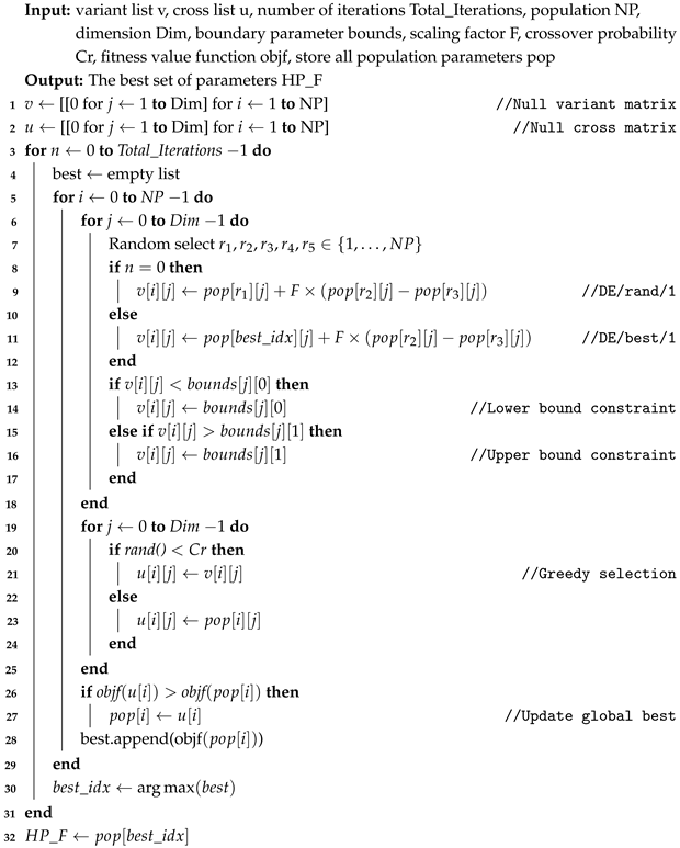
4.1. Data Selection and Processing

The data in this paper come from the actual sports test values of a university in 2022, and a total of 20,452 records were collected, covering the performance of students in physical fitness, skills, and comprehensive quality. To ensure both the accuracy and generalizability of the model, we systematically divided the dataset. A total of 70% of the data, that is, about 14,316 records, were allocated as the model training set. The remaining 30%, amounting to about 6136 records, were designated as the test set to validate and assess the performance and reliability of the trained model.

The existence of singular sample data in the sample data will affect the accuracy of the classification results to some extent [35]. In order to influence this part and enhance the precision of classification prediction outcomes, this paper adopts the max-min normalization method to normalize linear variables before establishing the model [36]. The calculation formula is shown in Equation (11):

$$Y={\displaystyle \frac{x-x_{\min }}{x_{\max }-x_{\min }}}$$

(11)

where x represents the original data value, $x_{\min }$ is the minimum value in the dataset, $x_{\max }$ is the maximum value in the dataset, and Y is the normalized data value ranging from 0 to 1.

4.2. Evaluation Index

In order to further compare the training results of the model and the actual application effect, this paper utilizes model evaluation indexes, such as the accuracy rate, recall rate, accuracy rate, ROC curve, and AUC value. These metrics facilitate a clearer visualization of the model’s predictive performance and generalization capability [37].

Accuracy rate is defined as the proportion of correctly predicted samples relative to the total number of samples. The higher the value, the better. Its calculation formula is shown in Equation (12):

$$\mathrm{A}={\displaystyle \frac{\mathrm{TP}+\mathrm{TN}}{\mathrm{TP}+\mathrm{TN}+\mathrm{FP}+\mathrm{FN}}}$$

(12)

where TP is the positive class sample correctly predicted by the model, TN is the negative class sample correctly predicted, FP is the positive class sample incorrectly predicted, and FN is the negative class sample incorrectly predicted.

Recall rate is defined as the proportion of predicted positive samples among those that are actually positive. A higher value indicates better performance. Its calculation formula is shown in Equation (13):

$$\mathrm{R}={\displaystyle \frac{\mathrm{TP}}{\mathrm{TP}+\mathrm{FN}}}$$

(13)

Accuracy rate refers to the proportion of predicted positive samples and actual positive samples. A higher value indicates better performance. Its calculation formula is shown in Equation (14):

$$\mathrm{P}={\displaystyle \frac{\mathrm{TP}}{\mathrm{TP}+\mathrm{FP}}}$$

(14)

The F1-score serves as a metric for evaluating classification problems. It represents the harmonic mean of precision and recall, with values ranging from 0 to 1. The calculation formula is shown in Equation (15):

$$\mathrm{F}1={\displaystyle \frac{2\times \mathrm{P}\times \mathrm{R}}{\mathrm{P}+\mathrm{R}}}$$

(15)

In the binary classification problem, P is the positive example and N is the negative example. T (true) means true and F (false) means not. TP denotes the count of samples that are genuinely positive and have been predicted as positive; FN signifies the count of samples that are genuinely positive but have been predicted as negative—for example, in the context of physical fitness testing, TP means that the actual physical fitness test result is a pass, and the predicted result is also a pass; FN indicates that the actual physical fitness test result is pass, but the predicted result is fail; FP indicates that the actual physical fitness test result is failing, but the predicted result is passing; TN indicates that the actual physical test result is failing, and the predicted result is also failing. The multi-classification problem can be transformed into the confusion matrix of the binary classification problem, as shown in

Table 3. Taking the physical fitness test as an example, a multi-classification transformation binary classification confusion matrix is presented.

Actual Result	Forecast Result
	Pass	Flunk
Pass	TP	FN
Flunk	FP	TN

.

The ROC curve, also known as the receiver operating characteristic curve (ROC) [38], is a comprehensive indicator of the continuous variables of the sensitivity and specificity of the response model. The ordinate TPR (true positive rate) refers to the “true positive rate” of samples. The horizontal coordinate FP (false positive rate) refers to the “false positive rate” of the sample. The coordinate point (0, 0) means that all samples are negative examples, the coordinate point (1, 1) means that all samples are positive examples, and the coordinate (0, 1) means perfect classification. The AUC value is the area enclosed under the ROC curve, and its value is between [0, 1]. The closer to 1, the better the classification effect.

4.3. Algorithm Comparison

In order to verify the performance of the algorithm, the DE-XGBoost model is compared with four models, XGBoost, SVM, GBM, and MLP, for a more comprehensive evaluation.

Table 4. Multi-index performance comparison under the F/Cr reverse combination.

	F = 0.1, Cr = 0.9	F = 0.3, Cr = 0.7	F = 0.5, Cr = 0.5	F = 0.7, Cr = 0.3	F = 0.9, Cr = 0.1
Accuracy rate	0.984444	0.9874442	0.987868	0.9875313	0.984791
Recall rate	0.984388	0.9874544	0.987889	0.9874556	0.984852
Precision rate	0.984714	0.9877286	0.988106	0.9878019	0.985062
F1	0.984311	0.9874137	0.987829	0.9874501	0.984750

shows the performance comparison of each index of the DE-XGBoost algorithm under different F/Cr reverse combinations, and

Table 5. Performance metrics with F = 0.5 under varying Cr values.

	F = 0.5, Cr = 0.1	F = 0.5, Cr = 0.3	F = 0.5, Cr = 0.5	F = 0.5, Cr = 0.7	F = 0.5, Cr = 0.9
Accuracy rate	0.986313	0.987770	0.987868	0.986955	0.986357
Recall rate	0.986385	0.987664	0.987889	0.987073	0.986615
Precision rate	0.986618	0.988071	0.988106	0.987163	0.986578
F1	0.986311	0.987656	0.987829	0.986948	0.986346

shows the impact of the Cr value on the performance of the DE-XGBoost model when F = 0.5 is fixed.

Table 6. Comparison of performance advantages of XGBoost model based on optimization algorithm.

	Accuracy Rate	Recall Rate	Precision Rate	F1
DE-XGBoost	0.987868	0.987889	0.988106	0.987829
PSO-XGBoost	0.985814	0.985899	0.986151	0.985813
SA-XGBoost	0.971356	0.971365	0.971876	0.970983

compares the performance advantages of XGBoost models under different optimization algorithms. The settings of the XGBoost, SVM and other model parameters are shown in

Table 7. Parameter setting of each model.

Algorithm	Argument
DE-XGBoost	NP = 15, Dim = 10, F = 0.5, Cr = 0.5
XGBoost	n_estimators = 100, learning_rate = 0.3, max_depth = 6, subsample = 1
SVM	C = 100, tol = 1 × 10−3, max_iter = −1, random_state = 42
GBM	n_estimators = 100, learning_rate = 0.1, max_depth = 3, random_state = 42
MLP	hidden_layer_sizes = 100, max_iter = 200, random_state = 42

, and the evaluation index data are shown in

Table 8. The results of physical testing and identification of each model.

	Accuracy Rate	Recall Rate	Precision Rate	F1
DE-XGBoost	0.987868	0.987889	0.988106	0.987829
XGBoost	0.952190	0.952138	0.951984	0.951564
SVM	0.908370	0.908370	0.908292	0.907966
GBM	0.945889	0.945889	0.946570	0.945136
MLP	0.938674	0.938674	0.938355	0.938212

.

Table 9. Friedman test.

Algorithm	Ranking
DE-XGBoost	1
XGBoost	2
SVM	5
GBM	3
MLP	4

shows the Friedman test’s resulting graph, showing each model’s performance ranking. The feature importance diagram of DE-XGBoost is shown in Figure 3. The ROC curve and AUC values of DE-XGBoost are shown in Figure 4. The confusion matrix for DE-XGBoost is shown in Figure 5. The confusion matrix normalization diagram of DE-XGBoost is shown in Figure 6. The convergence diagram of DE-XGBoost is shown in Figure 7.

Table 4 shows the impact of different parameter combinations of F and Cr on the performance of the DE-XGBoost model. The data indicate that the overall performance is optimal when F = 0.5 and Cr = 0.5 (accuracy 0.987868, F1-score 0.987829), while the performance is weakest when F = 0.1 and Cr = 0.9 (accuracy 0.984444, F1-score 0.984311). Although parameter adjustments cause fluctuations in the indicators, the maximum difference in accuracy is only 0.34%, and the overall impact is limited, especially when the suboptimal parameters (such as F = 0.3 and Cr = 0.7) have a difference of less than 0.05% compared to the optimal combination. Meanwhile, Table 5 shows that when F is fixed at 0.5, the parameter combination of F = 0.5 and Cr = 0.5 still performs optimally, while F = 0.5 and Cr = 0.9 performs the weakest (accuracy 0.986357). Notably, when Cr increases from 0.1 to 0.9, the fluctuation range of each indicator is relatively small, with the maximum difference in accuracy being 0.015, indicating that the adjustment of the Cr parameter also has a limited impact on the model performance under the current experimental settings. Therefore, adopting the optimal parameter combination (F = 0.5, Cr = 0.5) as determined in this paper can ensure performance while avoiding the complexity and resource consumption brought by adaptive algorithms.

According to the performance index comparison results presented in Table 6, the DE-XGBoost model demonstrates significant advantages in all four core evaluation dimensions: its prediction accuracy reaches as high as 0.987868, achieving a 0.2% and 1.7% improvement in accuracy compared to the improved versions based on Particle Swarm Optimization (PSO) and Simulated Annealing (SA), respectively; the recall rate and precision rate indicators both remain consistently above 0.98, reaching excellent performance of 0.987889 and 0.988106, respectively; and the F1 harmonic coefficient even reaches the optimally balanced value of 0.987829. This set of data fully validates the outstanding adaptability of the differential evolution algorithm in the hyperparameter optimization process of XGBoost. Through its efficient swarm intelligence search mechanism, it not only achieves breakthroughs in individual indicators but also significantly outperforms the traditional PSO and SA optimization schemes in the overall improvement of the model’s comprehensive predictive ability.

As shown in Table 7, DE-XGBoost performs joint optimization of 10 hyperparameters through differential evolution (NP = 15, F = 0.5, Cr = 0.5). Compared with the fixed parameters of traditional XGBoost (100 trees, 0.3 learning rate, depth 6), the accuracy rate of DE-XGBoost in Table 7 is improved by 3.6%. The advantages of evolutionary algorithms in the intelligent exploration of parameter space are verified. Among other models, SVM’s high regularization (C = 1.0) and RBF kernel are suitable for small samples but have high computational costs. The shallow structure of MLP (single hidden layer 50 nodes) and fixed learning rate (0.001) lead to weak generalization ability. GBM balances model complexity with convergence efficiency and is suitable for medium-scale data. DE-XGBoost’s auto-tuning benefits stand out when high precision and parallel resources are needed.

As evidenced by the evaluation index data presented in Table 8, there are certain differences in the performance of each model on the test set. The DE-XGBoost model performed best on all metrics, with accuracy, recall, accuracy and F1-scores all close to 0.988. This shows that DE-XGBoost is very effective in handling this task, with high predictive power and stability. The XGBoost model performed second, with accuracy, recall, accuracy, and F1-scores all around 0.952, slightly lower than DE-XGBoost, but still showing strong performance. The indicators of the SVM model are relatively low—all indicators are around 0.908, which represents a significant gap compared with DE-XGBoost. The GBM model was positioned between DE-XGBoost and SVM, with accuracy, recall, and F1-scores around 0.945. This shows that GBM is a relatively reliable model, but not as good as DE-XGBoost. The performance of the MLP is similar to GBM, but slightly lower, with all indicators around 0.938.

Table 9 presents the performance ranking of five algorithms, where DE-XGBoost takes the top spot with an absolute advantage, followed by XGBoost (2nd place) and GBM (3rd place), while MLP (4th place) and SVM (5th place) rank lower. This ranking indicates that DE-XGBoost performs the best in this evaluation. DE-XGBoost, with its optimized ensemble learning framework and feature-processing capabilities, leads to improved prediction accuracy and stability, demonstrating a significant advantage over the traditional tree models XGBoost and GBM in capturing non-linear relationships. In contrast, MLP and SVM, due to their sensitivity to data distribution and generalization limitations, rank at the bottom in this assessment, further highlighting the adaptability advantages of ensemble algorithms in complex tasks.

Figure 3 shows the feature importance scores derived from DE-XGBoost. Including gender (f1), height (f2), weight (f3), lung capacity (f4), 50 m run (f5), standing long jump (f6), sitting forward bend (f7), 800 m run (f8), 1000 m run (f9), 1 min sit-up (f10) and pull-up (f11), and 11 other characteristics. The X-axis represents the importance scores of the feature, and the Y-axis represents the names of the features. It can be intuitively seen from the figure that vital capacity (f4) and body weight (f3) are factors that affect classification accuracy, and the importance scores are 11,367.0 and 10,665.0, respectively. This is consistent with physiological research, which shows that respiratory efficiency and body composition directly affect health levels [39]. In contrast, sex (f1) showed the smallest effect, with a score of 168.0, suggesting that fitness classifications are less gender-biased in this dataset.

Figure 4 shows the ROC curve and AUC value of the DE-XGBoost model to reflect the characteristics of the model. Curve 1 represents excellent physical fitness, curve 2 indicates good physical fitness test performance, curve 3 indicates passing physical fitness test performance, and curve 4 indicates failing physical fitness test performance. The AUC value (area under the curve) is 0.99, close to 1.0, indicating that the DE-XGBoost model has extremely high accuracy and stability in distinguishing between different classes. The smoothness of the ROC curve and the trend towards the top-left corner further verify the excellent performance of the model in various categories.

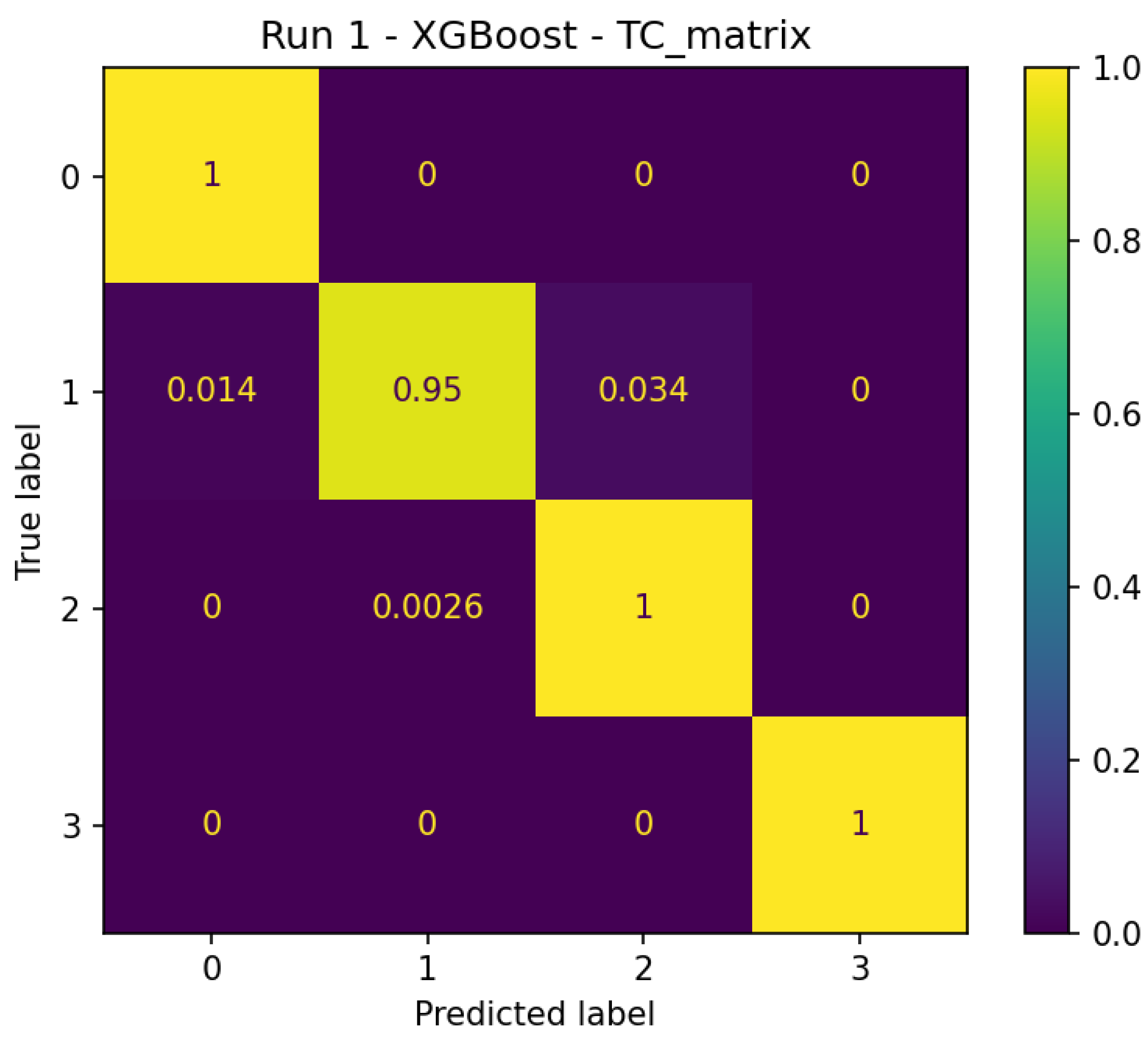
Figure 5 is a confusion matrix diagram of DE-XGBoost, showing the classification results of the model on the test set. As depicted in the figure, the classification performance of this model is excellent in most categories, especially categories 0 and 3, where the predicted results exhibit a high degree of consistency with the actual labels. The classification performance of category 1 is slightly weak, and there are some misclassification phenomena, but the overall performance is still good. For category 2, only a very small number of samples was misclassified. Figure 6 shows the normalized confusion matrix and the proportion of categories, in which 100% of the samples of category 0 are correctly predicted, the accuracy of category 1 is 95%, but there is a phenomenon that 3.4% is misjudged as category 2. Meanwhile, the distribution ratio of samples of categories 1 and 2 in the test set is close, indicating that the high accuracy of the model does not depend on the advantage of sample size, but has stable classification ability.

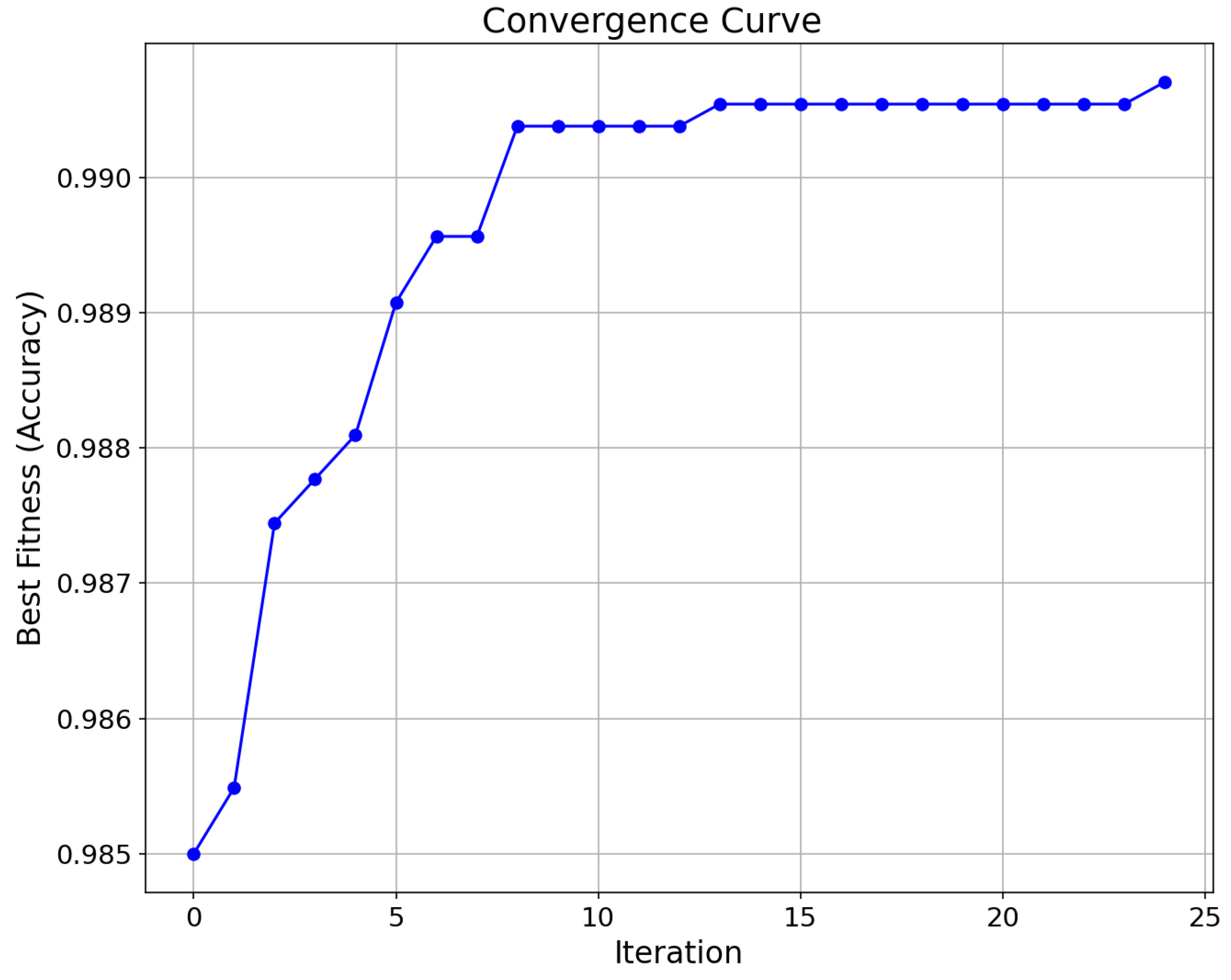
Figure 7 shows the convergence characteristics of the DE-XGBoost algorithm in the first run. The horizontal axis is the number of iterations (0–25), and the vertical axis is the best fitness (based on the classification accuracy index). The convergence curve presents a typical three-stage feature: the accuracy of the initial stage (0–5 iterations) rapidly rises from 0.985 to 0.990, reflecting the efficient exploration ability of the differential evolution mechanism in parameter space. In the middle stage (5–10 iterations), the upward slope is slow and accompanied by a small amount of fluctuation, reflecting the equilibrium process of development and exploration of the algorithm in the local optimal region. In the convergence stage (after 10 iterations), the accuracy rate is stable in the range of 0.990–0.992, and the fluctuation range is very small, which indicates that the hyperparameter combination of XGBoost has reached the approximate optimal configuration after 10 iterations. This convergence mode verifies the optimization efficiency of the DE-XGBoost framework, and only 10 iterations can be completed to optimize parameters while ensuring the model performance, significantly reducing the computational cost.

4.4. Sensitivity Analysis

To assess the influence of various data partitions on algorithm performance, multiple parameter combinations are employed to evaluate the effectiveness of the algorithm, which are respectively expressed as follows: (0.9, 0.1), (0.8, 0.2), (0.7, 0.3), (0.6, 0.4), (0.5, 0.5), (0.4, 0.6), (0.3, 0.7), (0.2, 0.8), (0.1, 0.9). The specific evaluation index results are shown in

Table 10. Sensitivity test.

Parameter	Accuracy Rate	Recall Rate	Precision Rate	F1
(0.9, 0.1)	0.991151	0.991148	0.991288	0.991108
(0.8, 0.2)	0.990052	0.990075	0.990249	0.990032
(0.7, 0.3)	0.987868	0.987889	0.988106	0.987829
(0.6, 0.4)	0.986215	0.986220	0.986465	0.986137
(0.5, 0.5)	0.983680	0.983684	0.983967	0.983590
(0.4, 0.6)	0.985777	0.985768	0.986053	0.985696
(0.3, 0.7)	0.976352	0.976326	0.976674	0.976156
(0.2, 0.8)	0.985710	0.985668	0.986016	0.985611
(0.1, 0.9)	0.957455	0.957459	0.957447	0.957053

. The results show that with the change in parameter combination, the performance of the algorithm exhibits a degree of fluctuation, and the overall performance basically shows a downward trend. When the parameter combination is (0.9, 0.1), the accuracy rate, recall rate, accuracy rate, and F1-score of the algorithm all achieve maximum metrics. With decrease in the first value and increase in the second value in the parameter combination, each index gradually decreases, especially when the parameter combination is (0.1, 0.9), and each index decreases significantly.

5. Conclusions

This paper proposes an innovative DE-XGBoost method to solve the problem of physical fitness test classification for college students. The proposed method optimizes the parameters of the XGBoost model by DE, which significantly boosts the algorithm’s performance in classifying physical test data. To validate the effectiveness of the DE-XGBoost method, we utilized a dataset comprising 20,452 physical test data collected in 2022 from a university as our experimental dataset. The results of our experiments demonstrate that, compared with other traditional and advanced classification algorithms, the DE-XGBoost method achieves significant improvement in classification accuracy, which not only validates the effectiveness of the DE-XGBoost method but also provides a new idea and technical means for the accurate classification of college students’ physical test data.

Although this paper has made some preliminary achievements in the classification of college students’ physical fitness test, it still has some shortcomings and needs to be expanded. This paper primarily concentrates on the optimization of XGBoost model parameters using DE but does not discuss other factors that may affect classification performance, such as data preprocessing and feature selection. Secondly, the data used in the experiment are relatively simple and do not involve more complex or diverse physical test data, which limits the full verification of the generalization capability of the DE-XGBoost method to a certain extent. Therefore, in future studies, we will work on higher-difficulty classification problems, such as multi-class classification or unbalanced data processing, and explore more complex feature engineering methods.