In the experimental section, for all complex optimization problems in CEC2011 and CEC2017, the number of evaluations was set to . In the corresponding data tables, “mean” and “std” represent the average value and standard deviation, respectively. W/T/L denotes the win/tie/loss comparison results under the Wilcoxon rank-sum test with a significance level of p = 0.05. After the standard deviation (std), +/=/− indicates the win/tie/loss relationship for that specific problem. The bold represents the best results. All experimental results are based on 51 independent runs on MATLAB R2024b.
5.2. Experimental Results and Analysis on External Comparison
In the field of intelligent optimization, DE has been widely applied to various continuous and mixed optimization problems due to its simple structure, few parameters, and strong global search capability. However, traditional DE and some of its early variants often face limitations such as an imbalance between exploitation and exploration capabilities and a tendency to fall into local optima when dealing with high-dimensional complex problems. To address these issues, numerous improved algorithms have been proposed in recent years, introducing innovations across multiple dimensions including evolutionary mechanisms, operator design, population control, and information guidance, thereby forming a rich evolutionary algorithm spectrum. To comprehensively evaluate the optimization capability of the proposed OLSHADE algorithm across different problem types and dimensions, and to verify the effectiveness of its core mechanisms, this study constructs a systematic external comparative experiment. The experiments carefully select nine representative high-performance optimization algorithms as comparison objects, covering several mainstream metaheuristic optimization paradigms. These include the latest variants within the frameworks of DE and particle swarm optimization (PSO), as well as emerging bio-inspired intelligence algorithms proposed in recent years, ensuring that the comparisons are both representative and challenging.
Regarding the testing platform, the experiments adopt two internationally recognized standard optimization test suites: CEC2017 and CEC2011. Among them, CEC2017 is a new-generation test platform proposed following multiple IEEE Congress on Evolutionary Computation (IEEE CEC) optimization competitions, focusing on evaluating the performance of EAs in theoretical complex function optimization. Its core objective is to build a systematic and hierarchical testing system to cover key capability requirements in optimization algorithm design. It includes unimodal, multimodal, composition, and hybrid problems across multiple problem dimensions, comprehensively testing the convergence ability, search breadth, and stability of algorithms. The CEC2011 test suite, published by the IEEE CEC, is designed to address the challenges of real-parameter optimization problems. Its goal is to construct a set of test functions with engineering backgrounds and complex structures to reflect common difficulties in real-world optimization tasks. This test suite contains 22 functions with dimensions ranging from 1 to 216, featuring high structural complexity, coupling, and diversity, as well as challenging characteristics, such as multi-scale, multi-modality, and non-differentiability, often present in real-world optimization scenarios. Therefore, CEC2011 places more emphasis on evaluating an algorithm’s adaptability and robustness in complex optimization problems within practical engineering environments. By jointly using these two standard benchmark sets, the experiments achieve a comprehensive evaluation of algorithm performance from both theoretical and application perspectives: CEC2017 provides a hierarchical, dimension-explicit theoretical verification platform suitable for assessing algorithm behavior under various basic function structures, while CEC2011 constructs a near-real evaluation environment under high uncertainty and complex interactions, helping to reveal algorithm stability and generalization capability in multidimensional hybrid-feature scenarios. This combination design establishes a performance evaluation framework with both breadth and depth, providing a rich experimental foundation for subsequent analysis.
In terms of the selection of comparative algorithms, this study focuses on representative cutting-edge algorithms published within the past five years, reflecting the foresight and contemporaneity of the experimental design. These algorithms can be broadly categorized into three groups.
First, algorithms based on DE constitute the primary comparison objects in this study. IMODE (2022) enhances global search capability and adaptability while maintaining DE’s structural simplicity by introducing multiple DE operators and integrating an operator weighting mechanism [
38]. DDEARA (2023) further expands into a distributed cooperative optimization framework, significantly improving multi-population parallel optimization efficiency by incorporating a performance-feedback-based resource allocation strategy and load-balancing scheduling [
39]. FODE (2025) innovatively introduces a fractional-order differential mechanism, strengthening DE’s modeling capability and global search performance in discrete and complex coupled problems [
36]. These algorithms represent key recent advancements in the DE paradigm in terms of operator fusion, resource scheduling, and mathematical modeling.
Second, improved algorithms based on PSO also play an important role in the experiments. TAPSO (2020) proposes a triple-archive learning model, enhancing convergence efficiency through particle learning mechanisms and learning path memory [
40]. AGPSO (2022) combines genetic learning with adaptive adjustment mechanisms to improve the algorithm’s search capability and result stability in real-world problems such as wind farm layout optimization [
41]. These two methods extend the exploration ability of traditional PSO from the perspectives of structural design and strategic guidance.
Third, the experiments also include several emerging metaheuristic algorithms developed rapidly in recent years, broadening the theoretical scope of the study. AHA (2022) simulates the multidirectional flight and foraging behavior of hummingbirds, constructing a novel algorithmic framework with three flight strategies and a foraging memory mechanism, demonstrating strong convergence performance [
42]. MCWFS (2025) builds a hierarchical population structure with elite, sub-elite, and memory collaboration systems, achieving a dynamic balance between exploitation and exploration through inter-level communication [
43]. SSAP (2023) improves the population control mechanism of the spherical search algorithm, effectively avoiding premature convergence and local optima by adaptively adjusting subpopulation size based on accumulated indicators [
44]. These algorithms demonstrate the diversity and evolutionary potential of metaheuristic algorithms from multiple perspectives, including bionic behavior modeling, cooperative structure design, and adaptive search control.
In summary, the experimental design of this study exhibits the following three prominent advantages: comprehensiveness, as reflected in the inclusion of comparison algorithms spanning DE, PSO, and various novel bio-inspired methods, representing both mainstream and innovative directions in current metaheuristic optimization; advancement, as all comparison algorithms were proposed after 2020, representing the current international frontier in optimization research; and rigor, as evidenced by the adoption of two standard benchmark test suites, CEC2017 and CEC2011, which consider both theoretical and engineering scenarios and encompass various dimensions and problem types, thereby establishing a complete and reproducible performance verification system. This experimental framework provides a solid and sufficient empirical basis for analyzing the advantages and applicability of the OLSHADE algorithm.
To thoroughly evaluate the overall performance of the proposed OLSHADE algorithm across various optimization complexities and dimensional scenarios, this study constructs a systematic external comparative experiment based on the CEC2017 test set, conducting direct performance comparisons with nine of the most representative current optimization algorithms. The selected comparative algorithms include OJADE, IMODE, DDEARA, FODE, SSAP, TAPSO, AGPSO, AHA, and MCWFS, covering emerging variants of DE and PSO, as well as various emerging metaheuristic algorithms in recent years. As shown in
Table 4,
Table 5,
Table 6,
Table 7,
Table 8,
Table 9,
Table 10,
Table 11,
Table 12 and
Table 13, the win/tie/loss (W/T/L) statistical indicator is employed for a comprehensive comparison across three test dimensions, 30, 50, and 100 dimensions, ensuring the conclusions possess broad applicability and credibility.
As shown in
Table 4 and
Table 5, in the 30-dimensional test scenario involving 30 problems, OLSHADE has demonstrated strong overall capabilities by achieving first place 18 times, second place 8 times, and third place 4 times. When facing high-performing DE variants such as OJADE (23 wins, 6 ties, 1 loss), IMODE (26 wins, 0 ties, 4 losses), and DDEARA (25 wins, 3 ties, 2 losses), OLSHADE achieved clear superiority on most functions, reflecting its innovative advantages in operator fusion and adaptive mechanism design. The comparison results with FODE (10 wins, 18 ties, 2 losses) and SSAP (13 wins, 13 ties, 4 losses) also indicate that OLSHADE possesses stable and dominant optimization capabilities under complex multimodal scenarios—although the tie ratio is high against FODE, the number of wins significantly exceeds the losses, suggesting overall superior performance without evident weaknesses. Notably, in comparisons with the recently prominent algorithms TAPSO, AGPSO, AHA, and MCWFS, OLSHADE achieved near-total victories: 28 wins and 2 losses; 30 wins and 0 losses; 29 wins, 0 ties, and 1 loss; and 30 wins and 0 losses, respectively, consistently outperforming under diverse function distributions and demonstrating the synergistic effect of diversity maintenance and convergence acceleration.
As shown in
Table 6,
Table 7 and
Table 8, among the 30 problems in 50 dimensions, with 18 first-place finishes, 7 second-place finishes, and 5 third-place finishes, OLSHADE further demonstrates its global search capability and adaptive robustness under increased dimensionality. Against OJADE (25 wins, 3 ties, 2 losses), IMODE (26 wins, 1 tie, 3 losses), and DDEARA (28 wins, 0 ties, 2 losses), it continues to achieve significant victories, indicating that its mechanism design maintains excellent generalization ability in high-dimensional spaces. In comparisons with FODE (10 wins, 18 ties, 2 losses) and SSAP (19 wins, 7 ties, 4 losses), OLSHADE similarly exhibits clear advantages: the number of wins far exceeds the number of losses, and it shows no disadvantage on any function, further validating its stable performance in search depth and function adaptability. Meanwhile, OLSHADE maintains a dominant position in comparisons with TAPSO (29 wins, 1 loss), AGPSO (30 wins, 0 losses), AHA (29 wins, 1 loss), and MCWFS (30 wins, 0 losses), achieving overwhelming superiority across all test functions and once again confirming the strength of its mechanisms and convergence performance in tackling complex high-dimensional optimization problems.
As shown in
Table 9,
Table 10 and
Table 11, in the most challenging 100-dimensional test scenario, OLSHADE demonstrated exceptional scalability and dimensional robustness by achieving first place 14 times, second place 9 times, and third place 7 times. The results against OJADE (21 wins, 2 ties, 7 losses) are relatively close, yet it maintains a clear advantage over IMODE (26 wins, 2 ties, 2 losses) and DDEARA (28 wins, 0 ties, 2 losses), indicating that its operator strategies and information-guided mechanisms are more adaptable to extremely high-dimensional spaces. When compared with FODE (17 wins, 9 ties, 4 losses) and SSAP (19 wins, 6 ties, 5 losses), the number of wins significantly exceeds the losses, further confirming that OLSHADE retains a stable global search advantage under the dual challenges of increased function complexity and dimensionality. In this set of tests, OLSHADE continues to maintain a comprehensive lead in comparisons with TAPSO (29 wins, 1 loss), AGPSO (30 wins, 0 losses), AHA (29 wins, 1 tie), and MCWFS (29 wins, 1 tie), showcasing its broad adaptability and performance across combinatorial and hybrid optimization problems.
Overall, OLSHADE exhibits leading optimization performance across all dimensionalities and function structures, with particularly outstanding results in complex combinatorial, high-dimensional multimodal, and disturbed hybrid-function scenarios. The synergistic integration of mechanisms such as multi-scale adaptive control, inter-individual information guidance, and local enhancement strategies significantly enhances global search depth and convergence accuracy, fully validating the theoretical innovativeness and empirical superiority of the proposed method.
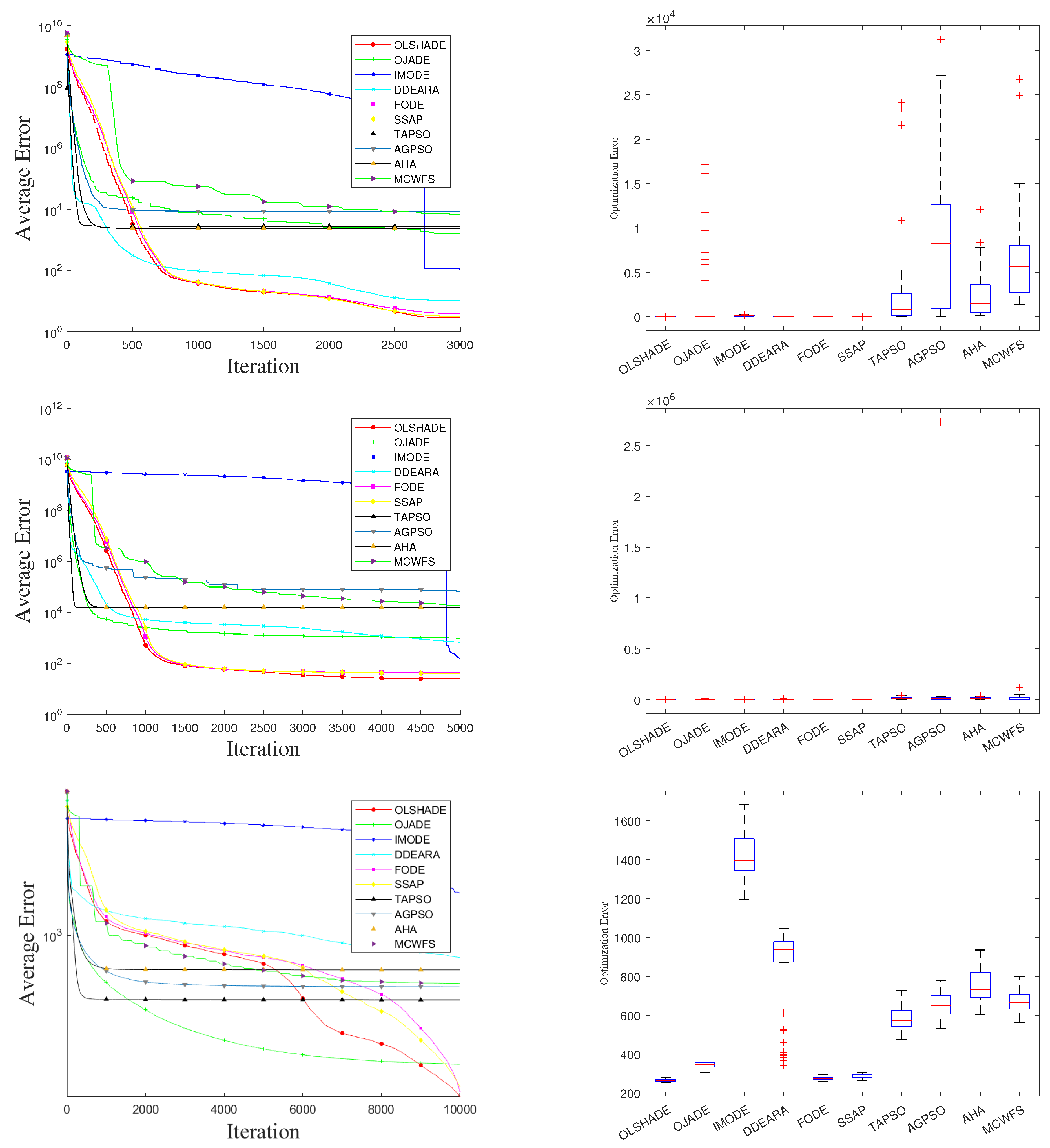
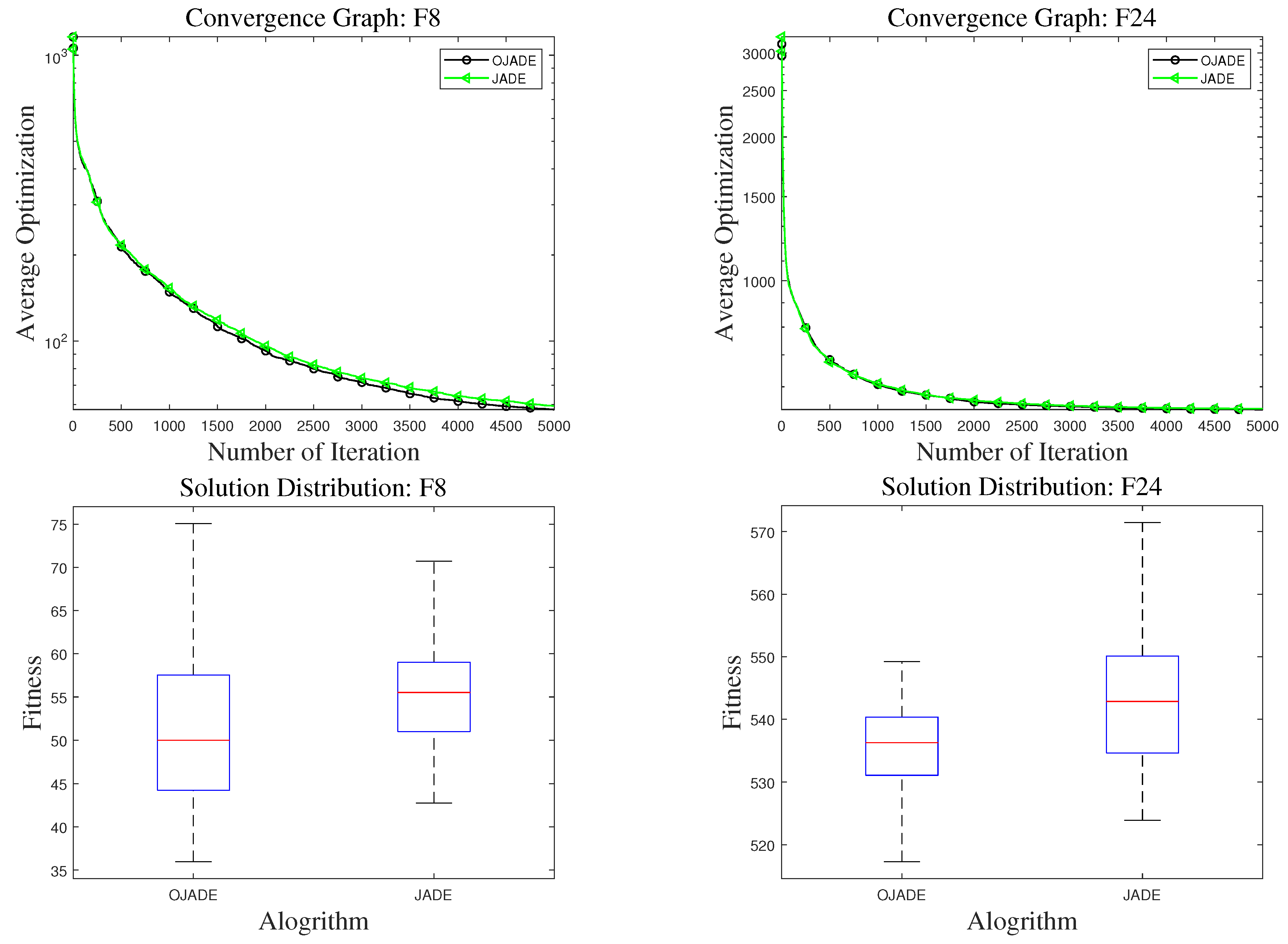
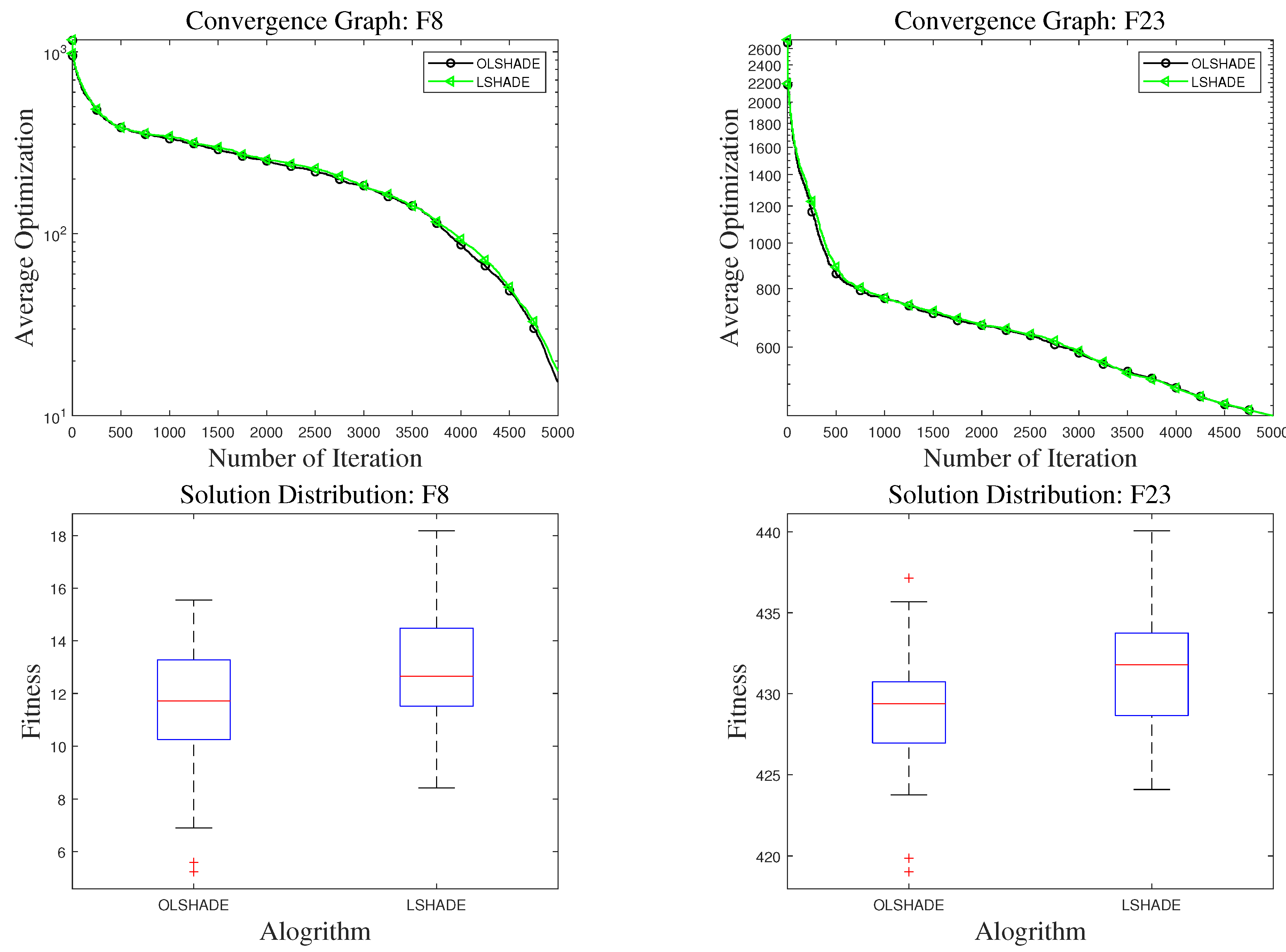
Furthermore, to validate the algorithm’s stability and global search performance throughout the iterative process from the perspectives of convergence efficiency and result distribution, this study also presents the convergence curves and box plots for representative functions. As shown in
Figure 7, the figure illustrates the variation of average error with the number of iterations for OLSHADE and the comparative algorithms on different problems in the 50-dimensional CEC2017 test tasks, along with statistical distributions of the final optimization results. The three groups of subplots correspond to three representative problems. From the convergence curves, it can be observed that OLSHADE exhibits faster descent rates and lower steady-state error levels in the vast majority of cases, indicating significant advantages in both convergence efficiency and solution accuracy.
Compared to improved DE algorithms such as OJDE and IMODE, OLSHADE maintains a leading performance during both the early rapid convergence phase and the later fine-tuning phase, further validating the effectiveness of its multi-scale adaptive search mechanism and local learning strategy. In contrast to PSO variants such as TAPSO and AGPSO, as well as emerging algorithms like AHA and MCWFS, OLSHADE demonstrates more stable convergence trends, avoiding issues such as premature stagnation or oscillatory convergence, thereby reflecting stronger convergence robustness. In the box plot analysis, OLSHADE consistently yields more concentrated result distributions with smaller variances across multiple tests, indicating higher consistency and stability in its optimization outcomes over repeated independent runs. By comparison, algorithms such as TAPSO and AGPSO show more outliers and larger variances, suggesting potential result volatility on specific problems. Although methods like MCWFS and FODE achieve relatively good results on certain functions, their overall distribution remains clearly inferior to that of OLSHADE. In summary, from convergence behavior to performance stability, OLSHADE demonstrates consistently strong and efficient advantages in the tests shown in
Figure 7, further supporting its comprehensive superiority in the aforementioned W/T/L statistical comparisons and validating the effectiveness and general applicability of the mechanisms proposed in this study at the performance level.
After demonstrating significant performance advantages in the three-dimensional test tasks of CEC2017, OLSHADE’s performance on the CEC2011 test set further validates its stability and effectiveness in solving complex problems in real-world engineering contexts. CEC2011 encompasses 22 continuous optimization functions of varying dimensions (ranging from 1 to 216), with complex and diverse problem structures that combine engineering relevance with highly nonlinear characteristics. It is commonly used to evaluate the generalization capability and robustness of optimization algorithms in practical environments.
As shown in
Table 12 and
Table 13, according to the w/t/l statistical results, OLSHADE achieved first place 10 times, second place 5 times, and third place 4 times. It achieved an absolute dominance over IMODE with 22 wins, 0 ties, and 0 losses across 22 functions, fully surpassing this improved DE algorithm. Against OJADE and TAPSO, it achieved 18 wins, 2 ties, and 2 losses, respectively, also demonstrating a significant advantage and stable dominance over these representative traditional DE and PSO methods. Against AGPSO and MCWFS, the results were 20 wins, 1 tie, 1 loss and 20 wins, 0 ties, 2 losses, respectively, maintaining a leading position and further illustrating the adaptability of its mechanism across various types of problems. Furthermore, although the performance gap between OLSHADE and DDEARA and AHA—two algorithms with strong adaptability mechanisms and balanced search designs—narrowed slightly (with results of 15 wins, 3 ties, 4 losses and 17 wins, 3 ties, 2 losses, respectively), OLSHADE still maintained a clear win-rate advantage, fully reflecting the robustness and generality of the introduced mechanism in engineering problems.
In comparisons with SSAP and FODE, OLSHADE achieved results of 2 wins, 12 ties, and 8 losses, and 4 wins, 12 ties, and 6 losses, respectively. Although OLSHADE did not secure an overall win advantage in these two comparisons, the high proportion of ties indicates that it maintained comparable or even superior performance to these two methods on the majority of problems. The underperformance on certain functions may be attributed to the strong function-structure adaptability of SSAP’s spherical search strategy and FODE’s fractional-order differential modeling, which offer inherent advantages under specific function characteristics (such as high coupling and robust constraint structures). Additionally, SSAP’s dynamic subpopulation size adjustment may be more favorable for addressing the wide dimensional span of functions in CEC2011, while FODE’s non-local search characteristics might be better suited for certain high-dimensional complex models.
However, it is important to emphasize that the performance advantages demonstrated by SSAP and FODE do not stem from irreproducible structural designs, but rather from analyzable and transferable algorithmic modules. Their core mechanisms—such as dynamic subpopulation control, fractional-order differential update strategies, and non-local jump search—possess good modularity and compatibility with other algorithms. More critically, OLSHADE is an enhancement based on the structurally concise LSHADE framework, with its core operator optimizations focused on strengthening the search mechanism and incorporating adaptive strategies. This “lightweight kernel + hierarchical optimization” design concept not only facilitates the independent validation of improvement strategies at the mechanism level but also retains high flexibility and plasticity for future algorithmic extensions. As a result, the mechanisms through which SSAP and FODE gain advantages on certain problems can theoretically be quickly integrated into the structurally open and highly pluggable OLSHADE framework in a modular manner. This characteristic enables OLSHADE not only to exhibit competitive performance at present but also to hold strong potential for continuous evolution and integration of other advanced strategies, providing a solid foundation for future research on complex optimization problems.
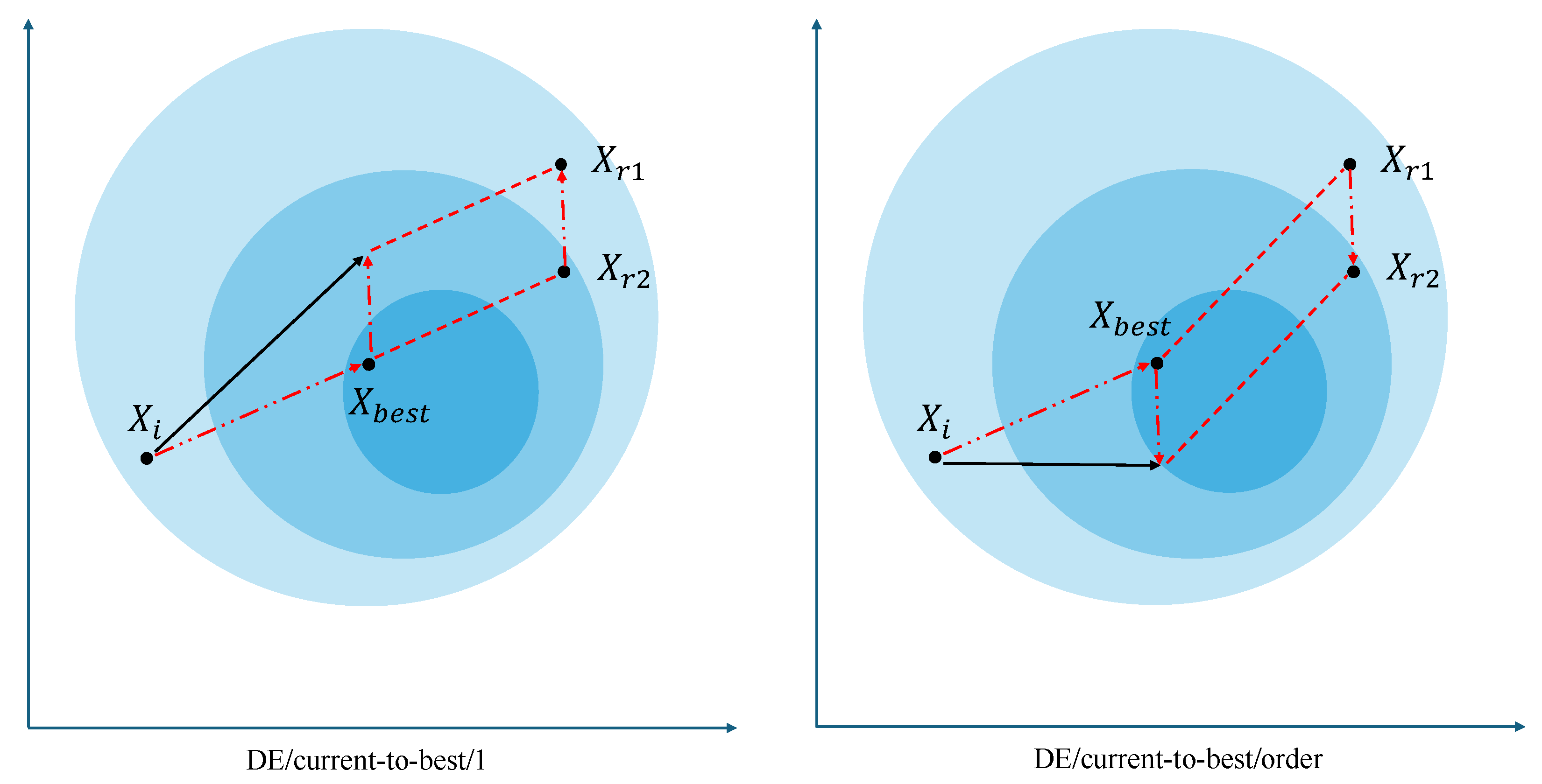
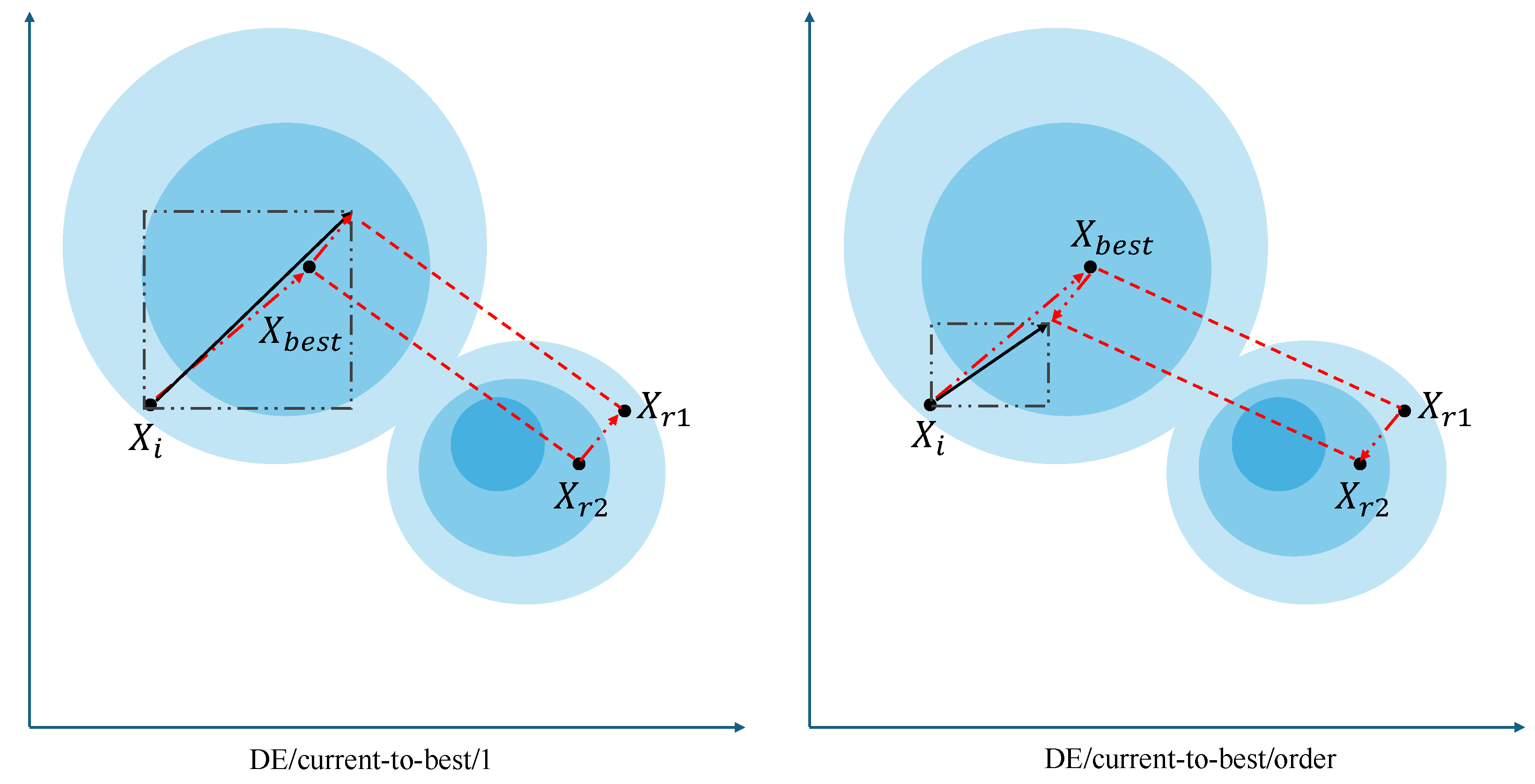
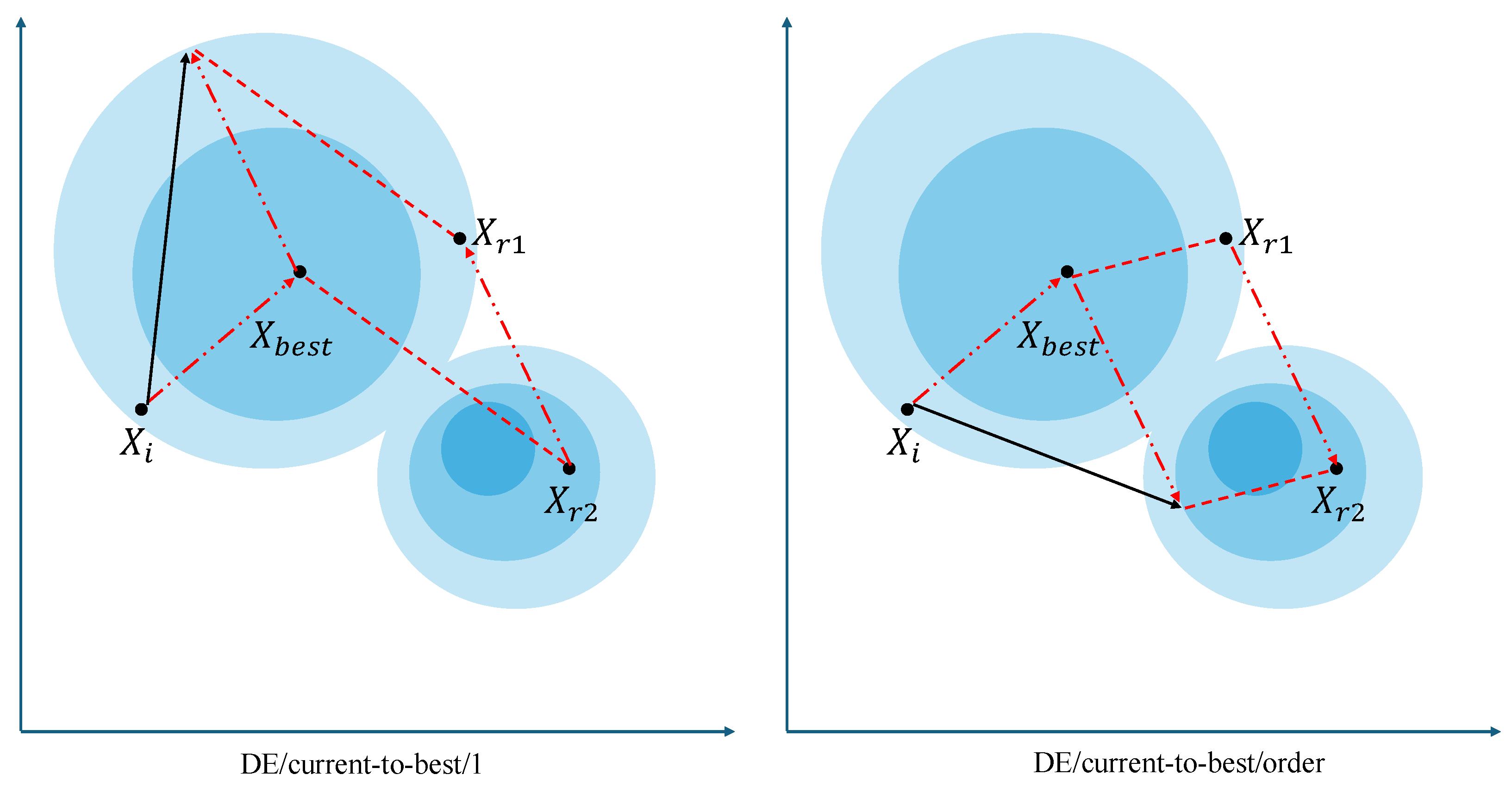
It is worth mentioning that both FODE and IMODE are representative methods that introduce other operator improvement mechanisms based on the LSHADE framework. They share the same main structure as the proposed OLSHADE, with the only difference lying in the differential mutation module employed. For this reason, these two algorithms are not only used as advanced comparative methods in this study, but the performance differences between them and OLSHADE can also be regarded as a form of external ablation-based structural validation. The experimental results obtained through this “same-framework, different-operator” comparative approach further verify that the proposed DE/current-to-pbest/order mechanism demonstrates superior performance over existing similar improvement strategies in complex constrained optimization problems, thereby providing cross-evidence support for its operator-level contribution independently of internal structural factors.
In summary, based on the overall results from both the CEC2011 and CEC2017 benchmark test sets, OLSHADE has demonstrated not only outstanding performance in theoretically structured function tests but also strong adaptability and stable output in complex optimization environments with engineering backgrounds. This validates the effectiveness, generality, and evolutionary potential of the proposed mechanisms across diverse optimization contexts.
5.3. Computational Complexity
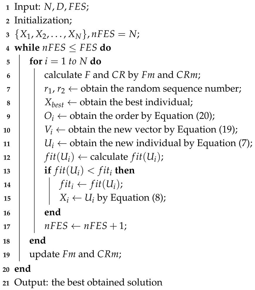
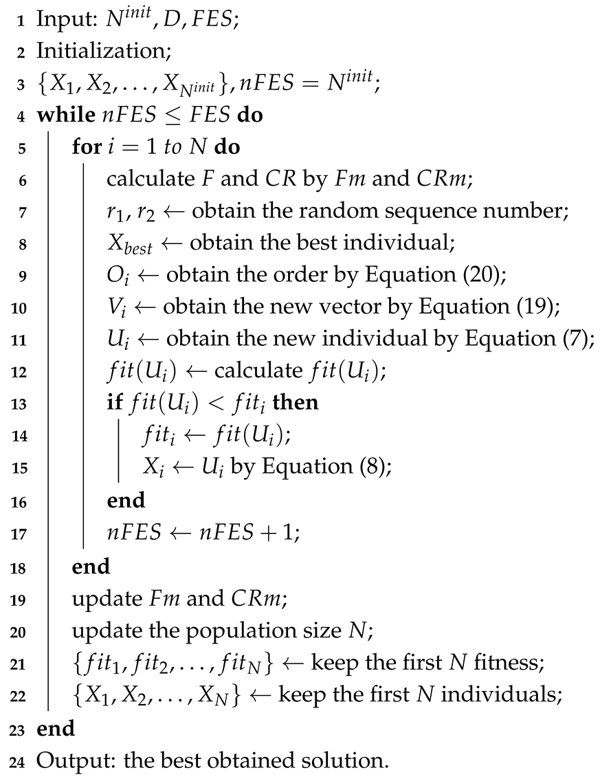
First, the order mechanism only adds a single constant-time fitness comparison operation and does not introduce any additional function evaluations. The DE/current-to-pbest/order operator proposed in this paper structurally differs from the traditional DE/current-to-pbest/1 only by the addition of a fitness comparison operation, which is used to construct the direction discrimination factor
:
This operation is a simple logical judgment with a computational complexity of , where the notation denotes the upper bound of asymptotic time complexity. Here, indicates that the execution time of this operation is constant, i.e., it does not increase with the growth of problem dimensionality D or population size N. Therefore, its runtime cost within the overall algorithm process is fixed and negligible, significantly lower than the cost of a single objective function evaluation. In our algorithm implementation, the fitness values of individuals are all computed and cached during the selection phase; thus, the comparison operation does not trigger any additional objective function evaluations, nor does it increase the number of function evaluations (FEs). Consequently, the operator proposed in this paper does not introduce any complexity increase at the function evaluation level or in the population evolution process, maintaining equivalence with the traditional DE algorithm in terms of basic resource requirements.
Second, the runtime efficiency test results indicate that the difference per unit time is minimal, the overall overhead is negligible, and a stable trend is maintained across all problem sets and dimensions. To further validate the “lightweight” nature of the order mechanism and enhance its applicability under “general problem scales and dimensional settings”, we conducted unified runtime measurements and analyses on all functions (a total of 30) in the complete CEC2017 benchmark test set under three typical dimensional settings (, , ). The specific test settings are as follows: all algorithms were executed on the same platform (Intel Core i7, 3.6 GHz, 32 GB RAM) implementation environment without parallel acceleration; all algorithms were independently repeated 30 times on each function and dimension; each run was performed under a fixed maximum number of function evaluations , ensuring equal computational budget across algorithms; we compared the runtime of OJADE vs. JADE and OLSHADE vs. LSHADE, with all algorithm parameters kept identical and the order mechanism being the only variable. The statistical results are as follows (all values are actual measured averages): at , OJADE shows an average runtime increase of 1.11% compared to JADE (5.243 s vs. 5.301 s), and OLSHADE shows an increase of 1.28% compared to LSHADE (6.328 s vs. 6.409 s); at , the average increases are 1.27% (8.212 s vs. 8.316 s) and 1.41% (8.964 s vs. 9.090 s), respectively; at , the increases are 1.38% (10.573 s vs. 10.719 s) and 1.56% (12.379 s vs. 12.572 s), respectively. The trend in standard deviation changes indicates stable runtime performance without significant fluctuations or differences across functions. It is noteworthy that these differences mainly stem from the order mechanism introducing a simple scalar comparison operation, rather than additional iteration procedures or function evaluations. Thus, its impact on total runtime is strictly limited by the number of iterations and population size and does not scale with changes in the problem function properties. Moreover, since the order mechanism does not introduce any learning modules, matrix operations, or additional structural complexity, it does not incur nonlinear time growth with increasing problem dimensionality.
Therefore, we conclude that the mechanism demonstrates highly stable cost-control capability across three typical dimensional settings and the entire problem set, and its “lightweight” structural characteristics are validated under the complete testing scenarios. Compared with many adaptive mechanisms that introduce historical sample evaluation, archive search, or parameter learning modules, the computational overhead introduced by the order mechanism constitutes a “constant-level perturbation”, which is entirely negligible in optimization contexts where the main computational load lies in function evaluations. This conclusion further substantiates the appropriateness of our use of the term “lightweight”, and it is supported by both cross-method comparison and practical applicability in engineering deployment scenarios.
Third, the design rationale of the “lightweight” definition is as follows: minimal structure, no additional parameters, and no external component dependencies. In addition to the quantitative explanation from the perspective of runtime efficiency, the proposed order mechanism also adheres to the following lightweight design principles, further reinforcing the structural basis for the “lightweight” characterization:
Structural minimalism: The operator is embedded directly within the basic mutation construction of DE, without introducing new modules.
Zero parameter addition: No control parameters, adjustment factors, or fitness weighting coefficients are introduced, thereby reducing the parameter tuning burden.
No data dependency: The mechanism does not rely on historical populations, distribution information, or memory archives, leaving the algorithm’s time and space complexity unchanged.
High integrability: It can be seamlessly embedded into any standard DE framework, offering good adaptability and low deployment cost.
This design philosophy is markedly distinct from many improved algorithms that adopt learning-based strategies (such as adaptive weights, covariance matrix estimation, or sample selectors). As a result, the order mechanism not only demonstrates strong theoretical simplicity but also offers greater suitability for deployment in tasks that are resource-sensitive or have complex operational environments.
Table 4.
Experiment results of OLSHADE and comparative algorithms on IEEE CEC2017 (D = 30).
Table 4.
Experiment results of OLSHADE and comparative algorithms on IEEE CEC2017 (D = 30).
| Algorithm | F1 | F2 | F3 |
| OLSHADE | 0.000E+00 ± 0.000E+00 | 0.000E+00 ± 0.000E+00 | 0.000E+00 ± 0.000E+00 |
| OJADE | 0.000E+00 ± 0.0000E+00≈ | 0.000E+00 ± 0.0000E+00≈ | 9.313E+03 ± 1.703E+04 + |
| IMODE | 9.104E−03 ± 1.751E−03 + | 3.014E+01 ± 1.801E+02 + | 1.920E−07 ± 5.003E−09 + |
| DDEARA | 2.648E+02 ± 3.227E+02 + | 3.852E+09 ± 4.634E+09 + | 5.708E+01 ± 5.629E+01 + |
| FODE | 0.000E+00 ± 0.000E+00≈ | 0.000E+00 ± 0.000E+00≈ | 0.000E+00 ± 0.000E+00≈ |
| SSAP | 0.000E+00 ± 0.000E+00≈ | 0.000E+00 ± 0.000E+00≈ | 0.000E+00 ± 0.000E+00≈ |
| TAPSO | 2.216E+03 ± 3.142E+03 + | 7.202E−
05 ± 1.447E−
04 + | 0.000E+00 ± 0.000E+00≈ |
| AGPSO | 9.855E+04 ± 4.741E+05 + | 3.432E+24 ± 1.436E+25 + | 2.191E+04 ± 5.145E+03 + |
| AHA | 3.804E+03 ± 4.697E+03 + | 5.047E+05 ± 2.651E+06 + | 2.677E+01 ± 4.543E+01 + |
| MCWFS | 4.276E+03 ± 4.200E+03 + | 1.016E+06 ± 4.190E+06 + | 2.336E−01 ± 2.783E−01 + |
| Algorithm | F4 | F5 | F6 |
| OLSHADE | 5.878E+01 ± 1.089E+00 | 6.355E+00 ± 1.516E+00 | 4.035E-09 ± 2.015E-08 |
| OJADE | 5.136E+01 ± 2.219E+01 + | 2.827E+01 ± 3.993E+00 + | 0.000E+00 ± 0.000E+00− |
| IMODE | 1.146E+01 ± 2.175E+01− | 9.258E+01 ± 2.002E+01 + | 9.787E+00 ± 2.669E+00 + |
| DDEARA | 8.284E+01 ± 2.487E+01 + | 7.213E+01 ± 1.152E+01 + | 0.000E+00 ± 0.000E+00− |
| FODE | 5.856E+01 ± 1.392E−
14 − | 6.573E+00 ± 1.465E+00 ≈ | 6.711E−
09 ± 2.739E−
08 ≈ |
| SSAP | 3.585E+01 ± 3.009E+01 ≈ | 9.676E+00 ± 1.932E+00 + | 8.722E−09 ± 3.271E−08 ≈ |
| TAPSO | 3.673E+01 ± 2.885E+01 ≈ | 4.711E+01 ± 1.178E+01 + | 1.238E−
03 ± 1.671E−03 + |
| AGPSO | 2.914E+02 ± 9.243E+01 + | 1.761E+02 ± 1.916E+01 + | 5.087E+00 ± 2.062E+00 + |
| AHA | 8.081E+01 ± 3.084E+01 + | 1.071E+02 ± 2.353E+01 + | 2.464E−01 ± 5.292E−01 + |
| MCWFS | 8.043E+01 ± 2.464E+01 + | 6.645E+01 ± 1.702E+01 + | 3.159E+00 ± 2.555E+00 + |
| Algorithm | F7 | F8 | F9 |
| OLSHADE | 3.757E+01 ± 1.283E+00 | 7.105E+00 ± 1.236E+00 | 0.000E+00 ± 0.000E+00 |
| OJADE | 5.482E+01 ± 3.106E+00 + | 2.517E+01 ± 3.670E+00 + | 0.000E+00 ± 0.000E+00≈ |
| IMODE | 1.580E+02 ± 2.741E+01 + | 9.049E+01 ± 1.327E+01 + | 1.078E+03 ± 3.404E+02 + |
| DDEARA | 1.140E+02 ± 1.108E+01 + | 7.545E+01 ± 1.113E+01 + | 4.522E−
03 ± 1.847E−
02 + |
| FODE | 3.743E+01 ± 1.306E+00≈ | 7.124E+00 ± 1.477E+00 ≈ | 0.000E+00 ± 0.000E+00≈ |
| SSAP | 3.889E+01 ± 1.735E+00 + | 9.399E+00 ± 1.437E+00 + | 0.000E+00 ± 0.000E+00≈ |
| TAPSO | 7.405E+01 ± 1.544E+01 + | 4.313E+01 ± 1.087E+01 + | 1.415E+01 ± 2.048E+01 + |
| AGPSO | 1.620E+02 ± 5.406E+01 + | 1.535E+02 ± 3.818E+01 + | 1.409E+01 ± 9.247E+00 + |
| AHA | 1.437E+02 ± 3.558E+01 + | 1.051E+02 ± 2.424E+01 + | 1.361E+03 ± 9.709E+02 + |
| MCWFS | 9.825E+01 ± 1.457E+01 + | 6.307E+01 ± 1.348E+01 + | 9.448E+00 ± 9.583E+00 + |
| Algorithm | F10 | F11 | F12 |
| OLSHADE | 1.387E+03 ± 2.354E+02 | 3.128E+01 ± 2.845E+01 | 1.069E+03 ± 4.011E+02 |
| OJADE | 1.866E+03 ± 2.472E+02 + | 3.115E+01 ± 2.429E+01 + | 1.220E+03 ± 3.989E+02 + |
| IMODE | 2.589E+03 ± 4.650E+02 + | 1.320E+02 ± 4.943E+01 + | 1.224E+03 ± 3.897E+02 + |
| DDEARA | 3.669E+03 ± 3.792E+02 ≈ | 1.379E+01 ± 1.356E+01 + | 2.349E+04 ± 1.221E+04 + |
| FODE | 1.393E+03 ± 2.169E+02 ≈ | 3.913E+01 ± 2.851E+01 + | 1.124E+03 ± 3.646E+02 ≈ |
| SSAP | 1.736E+03 ± 1.959E+02 + | 1.805E+01 ± 2.405E+01≈ | 1.083E+03 ± 3.783E+02 ≈ |
| TAPSO | 2.523E+03 ± 5.942E+02 + | 7.674E+01 ± 3.816E+01 + | 2.206E+04 ± 1.347E+04 + |
| AGPSO | 6.542E+03 ± 3.351E+02 + | 1.322E+02 ± 6.007E+01 + | 7.840E+06 ± 1.328E+07 + |
| AHA | 3.245E+03 ± 6.450E+02 + | 6.608E+01 ± 2.801E+01 + | 1.152E+05 ± 9.365E+04 + |
| MCWFS | 2.371E+03 ± 4.400E+02 + | 1.009E+02 ± 3.197E+01 + | 1.786E+05 ± 2.096E+05 + |
Table 5.
Experiment results of OLSHADE and comparative algorithms on IEEE CEC2017 (D = 30).
Table 5.
Experiment results of OLSHADE and comparative algorithms on IEEE CEC2017 (D = 30).
| Algorithm | F13 | F14 | F15 |
| OLSHADE | 1.673E+01 ± 4.448E+00 | 2.169E+01 ± 1.321E+00 | 2.810E+00 ± 1.734E+00 |
| OJADE | 2.040E+02 ± 1.229E+03 + | 6.188E+03 ± 1.130E+04 + | 1.555E+03 ± 4.026E+03 + |
| IMODE | 2.449E+02 ± 1.043E+02 + | 1.373E+02 ± 4.446E+01 + | 1.098E+02 ± 4.257E+01 + |
| DDEARA | 3.319E+02 ± 6.968E+02 ≈ | 2.295E+01 ± 1.752E+01 + | 1.018E+01 ± 5.235E+00 + |
| FODE | 1.722E+01 ± 4.803E+00 ≈ | 2.191E+01 ± 1.355E+00 ≈ | 3.854E+00 ± 1.885E+00 + |
| SSAP | 1.685E+01 ± 6.193E+00 ≈ | 2.191E+01 ± 3.284E+00 + | 3.142E+00 ± 1.655E+00 ≈ |
| TAPSO | 1.492E+04 ± 1.377E+04 + | 2.206E+03 ± 4.377E+03 + | 2.740E+03 ± 5.541E+03 + |
| AGPSO | 5.504E+04 ± 2.297E+05 + | 3.526E+04 ± 8.101E+04 + | 8.491E+03 ± 8.313E+03 + |
| AHA | 1.165E+04 ± 1.027E+04 + | 1.243E+03 ± 1.541E+03 + | 2.308E+03 ± 2.436E+03 + |
| MCWFS | 2.015E+04 ± 1.241E+04 + | 1.967E+02 ± 4.116E+01 + | 6.704E+03 ± 5.253E+03 + |
| Algorithm | F16 | F17 | F18 |
| OLSHADE | 4.246E+01 ± 4.153E+01 | 3.242E+01 ± 5.957E+00 | 2.175E+01 ± 9.353E−
01 |
| OJADE | 4.1698E+02 ± 1.3342E+02 + | 6.8643E+01 ± 1.7497E+01 + | 5.3373E+03 ± 2.8839E+04 + |
| IMODE | 6.631E+02 ± 2.031E+02 + | 1.901E+02 ± 8.919E+01 + | 8.212E+01 ± 2.599E+01 + |
| DDEARA | 5.032E+02 ± 1.715E+02 + | 5.966E+01 ± 5.315E+01 + | 2.931E+03 ± 3.146E+03 + |
| FODE | 5.832E+01 ± 5.995E+01 ≈ | 3.326E+01 ± 5.435E+00 ≈ | 2.272E+01 ± 1.948E+00 + |
| SSAP | 2.147E+02 ± 9.313E+01 + | 3.702E+01 ± 6.470E+00 + | 2.250E+01 ± 1.588E+00 + |
| TAPSO | 6.990E+02 ± 2.892E+02 + | 2.067E+02 ± 1.220E+02 + | 5.034E+04 ± 2.632E+04 + |
| AGPSO | 1.359E+03 ± 2.055E+02 + | 2.777E+02 ± 1.646E+02 + | 6.947E+05 ± 7.499E+05 + |
| AHA | 9.237E+02 ± 2.804E+02 + | 3.425E+02 ± 1.865E+02 + | 2.115E+04 ± 1.339E+04 + |
| MCWFS | 4.530E+02 ± 1.733E+02 + | 1.459E+02 ± 7.120E+01 + | 2.428E+04 ± 1.406E+04 + |
| Algorithm | F19 | F20 | F21 |
| OLSHADE | 5.047E+00 ± 1.516E+00 | 3.040E+01 ± 7.304E+00 | 2.070E+02 ± 1.833E+00 |
| OJADE | 1.407E+03 ± 3.727E+03 + | 1.100E+02 ± 5.601E+01 + | 2.260E+02 ± 4.524E+00 + |
| IMODE | 2.208E+02 ± 7.484E+01 + | 1.354E+02 ± 7.375E+01 + | 1.012E+02 ± 1.717E+00− |
| DDEARA | 6.331E+00 ± 2.280E+00 + | 5.987E+01 ± 6.539E+01 ≈ | 2.781E+02 ± 1.210E+01 + |
| FODE | 5.941E+00 ± 1.750E+00 + | 3.501E+01 ± 5.533E+00 + | 2.071E+02 ± 1.441E+00 ≈ |
| SSAP | 5.271E+00 ± 1.893E+00 ≈ | 5.777E+01 ± 1.513E+01 + | 2.087E+02 ± 1.701E+00 + |
| TAPSO | 5.169E+03 ± 5.028E+03 + | 2.782E+02 ± 1.547E+02 + | 2.498E+02 ± 1.477E+01 + |
| AGPSO | 9.548E+03 ± 1.393E+04 + | 2.793E+02 ± 1.377E+02 + | 3.743E+02 ± 2.345E+01 + |
| AHA | 3.747E+03 ± 3.045E+03 + | 3.408E+02 ± 1.380E+02 + | 2.720E+02 ± 1.529E+01 + |
| MCWFS | 7.107E+03 ± 1.163E+04 + | 2.436E+02 ± 9.637E+01 + | 2.597E+02 ± 1.314E+01 + |
| Algorithm | F22 | F23 | F24 |
| OLSHADE | 1.000E+02 ± 1.005E−
13 + | 3.499E+02 ± 2.3255E+00 + | 4.259E+02 ± 1.666E+00 + |
| OJADE | 1.000E+02 ± 1.005E−
13 ≈ | 3.718E+02 ± 6.519E+00 + | 4.392E+02 ± 4.512E+00 + |
| IMODE | 4.556E+02 ± 2.966E+01 + | 5.735E+02 ± 9.761E+01 + | 7.249E+01 ± 2.508E+01− |
| DDEARA | 1.000E+02 ± 0.000E+00− | 4.243E+02 ± 1.425E+01 + | 5.127E+02 ± 2.336E+01 + |
| FODE | 1.000E+02 ± 1.435E−
14 ≈ | 3.498E+02 ± 2.656E+00 ≈ | 4.256E+02 ± 1.904E+00 + |
| SSAP | 1.000E+02 ± 1.435E−14 ≈ | 3.452E+02 ± 3.302E+00− | 4.213E+02 ± 2.086E+00 − |
| TAPSO | 4.780E+02 ± 9.702E+02 + | 4.157E+02 ± 2.003E+01 + | 4.977E+02 ± 2.264E+01 + |
| AGPSO | 1.021E+02 ± 2.319E+00 + | 5.930E+02 ± 2.099E+01 + | 6.565E+02 ± 2.180E+01 + |
| AHA | 1.006E+02 ± 1.274E+00 + | 4.383E+02 ± 2.768E+01 + | 5.076E+02 ± 2.818E+01 + |
| MCWFS | 1.000E+02 ± 1.525E−02 + | 4.157E+02 ± 1.555E+01 + | 4.735E+02 ± 1.452E+01 + |
| Algorithm | F25 | F26 | F27 |
| OLSHADE | 3.867E+02 ± 2.475E−02 | 9.146E+02 ± 3.527E+01 | 5.022E+02 ± 5.631E+00 |
| OJADE | 3.870E+02 ± 1.493E−
01 + | 1.174E+03 ± 7.331E+01 + | 5.028E+02 ± 6.544E+00 ≈ |
| IMODE | 3.914E+02 ± 1.343E+01 + | 2.843E+02 ± 3.673E+01 − | 5.466E+02 ± 1.178E+01 + |
| DDEARA | 3.864E+02 ± 1.206E+00 + | 1.326E+03 ± 4.614E+02 + | 5.063E+02 ± 7.367E+00 + |
| FODE | 3.867E+02 ± 1.683E−
02 ≈ | 9.162E+02 ± 3.717E+01 ≈ | 5.036E+02 ± 5.544E+00 ≈ |
| SSAP | 3.868E+02 ± 2.889E−02 + | 8.927E+02 ± 5.145E+01 − | 5.036E+02 ± 6.897E+00 ≈ |
| TAPSO | 3.883E+02 ± 5.658E+00 + | 1.442E+03 ± 6.121E+02 + | 5.175E+02 ± 1.158E+01 + |
| AGPSO | 4.330E+02 ± 2.126E+01 + | 2.945E+03 ± 9.361E+02 + | 6.666E+02 ± 2.153E+01 + |
| AHA | 3.963E+02 ± 1.523E+01 + | 7.638E+02 ± 1.081E+03− | 5.425E+02 ± 1.504E+01 + |
| MCWFS | 3.873E+02 ± 2.454E+00 + | 1.476E+03 ± 4.442E+02 + | 5.180E+02 ± 1.354E+01 + |
| Algorithm | F28 | F29 | F30 |
| OLSHADE | 3.310E+02 ± 5.136E+01 | 4.307E+02 ± 5.468E+00 | 1.988E+03 ± 5.345E+01 |
| OJADE | 3.305E+02 ± 5.091E+01 ≈ | 4.800E+02 ± 1.917E+01 + | 2.262E+03 ± 1.100E+03 + |
| IMODE | 3.299E+02 ± 5.577E+01 + | 6.863E+02 ± 9.191E+01 + | 3.213E+03 ± 7.184E+02 + |
| DDEARA | 4.024E+02 ± 1.621E+01 + | 5.229E+02 ± 6.971E+01 + | 3.361E+03 ± 1.271E+03 + |
| FODE | 3.279E+02 ± 4.875E+01 ≈ | 4.320E+02 ± 6.806E+00 ≈ | 1.992E+03 ± 6.255E+01 ≈ |
| SSAP | 3.105E+02 ± 3.235E+01− | 4.413E+02 ± 7.007E+00 + | 2.069E+03 ± 6.809E+01 + |
| TAPSO | 3.296E+02 ± 5.472E+01 + | 6.323E+02 ± 1.713E+02 + | 4.914E+03 ± 2.782E+03 + |
| AGPSO | 5.465E+02 ± 7.722E+01 + | 8.682E+02 ± 1.783E+02 + | 9.170E+04 ± 1.539E+05 + |
| AHA | 4.043E+02 ± 1.871E+01 + | 7.038E+02 ± 1.582E+02 + | 4.779E+03 ± 1.701E+03 + |
| MCWFS | 3.614E+02 ± 4.767E+01 + | 5.965E+02 ± 7.869E+01 + | 1.346E+05 ± 1.151E+05 + |
| Algorithm | | | |
| OLSHADE | − | | |
| OJADE | 23/6/1 | | |
| IMODE | 26/0/4 | | |
| DDEARA | 25/3/2 | | |
| FODE | 6/23/1 | | |
| SSAP | 13/13/4 | | |
| TAPSO | 28/2/0 | | |
| AGPSO | 30/0/0 | | |
| AHA | 29/0/1 | | |
| MCWFS | 30/0/0 | | |
Table 6.
Experiment results of OLSHADE and comparative algorithms on IEEE CEC2017 (D = 50).
Table 6.
Experiment results of OLSHADE and comparative algorithms on IEEE CEC2017 (D = 50).
| Algorithm | F1 | F2 | F3 |
| OLSHADE | 0.000E+00 ± 0.000E+00 | 0.000E+00 ± 0.000E+00 | 0.000E+00 ± 0.000E+00 |
| OJADE | 0.000E+00 ± 0.000E+00≈ | 3.800E−10 ± 2.714E−09 ≈ | 1.713E+04 ± 3.537E+04 + |
| IMODE | 1.582E−02 ± 1.369E−03 + | 7.030E+31 ± 4.278E+32 + | 9.578E−07 ± 4.812E−08 + |
| DDEARA | 1.383E+03 ± 1.676E+03 + | 9.806E+09 ± 1.384E+09 + | 3.547E+01 ± 1.733E+02 + |
| FODE | 0.000E+00 ± 0.000E+00≈ | 0.000E+00 ± 0.000E+00≈ | 0.000E+00 ± 0.000E+00≈ |
| SSAP | 0.000E+00 ± 0.000E+00≈ | 0.000E+00 ± 0.000E+00≈ | 0.000E+00 ± 0.000E+00≈ |
| TAPSO | 3.330E+03 ± 4.628E+03 + | 2.574E-05 ± 4.529E-05 + | 7.109E+01 ± 1.838E+02 + |
| AGPSO | 6.138E+06 ± 4.045E+07 + | 7.731E+52 ± 5.483E+53 + | 7.827E+04 ± 1.101E+04 + |
| AHA | 2.870E+03 ± 3.387E+03 + | 1.233E+12 ± 3.396E+12 + | 1.215E+03 ± 7.699E+02 + |
| MCWFS | 7.205E+03 ± 6.452E+03 + | 1.042E+13 ± 5.386E+13 + | 6.751E+00 ± 2.415E+00 + |
| Algorithm | F4 | F5 | F6 |
| OLSHADE | 7.348E+01 ± 5.120E+01 | 1.119E+01 ± 2.158E+00 | 9.831E−08 ± 1.827E−07 |
| OJADE | 5.575E+01 ± 4.882E+01 ≈ | 4.717E+01 ± 8.456E+00 + | 0.000E+00 ± 0.000E+00− |
| IMODE | 3.217E+01 ± 4.497E+01− | 2.860E+02 ± 3.159E+01 + | 3.473E+01 ± 5.506E+00 + |
| DDEARA | 1.102E+02 ± 4.348E+01 + | 2.163E+02 ± 2.068E+01 + | 0.000E+00 ± 0.000E+00 − |
| FODE | 8.403E+01 ± 4.355E+01 ≈ | 1.237E+01 ± 2.333E+00 + | 4.190E−05 ± 2.984E−04 ≈ |
| SSAP | 3.375E+01 ± 4.343E+01 − | 2.342E+01 ± 2.085E+00 + | 7.759E-04 ± 2.181E-03 + |
| TAPSO | 4.704E+01 ± 4.271E+01 − | 1.135E+02 ± 2.844E+01 + | 8.111E-03 ± 6.440E-03 + |
| AGPSO | 8.643E+02 ± 2.489E+02 + | 3.566E+02 ± 4.186E+01 + | 1.472E+01 ± 2.961E+00 + |
| AHA | 1.067E+02 ± 4.738E+01 + | 2.921E+02 ± 3.396E+01 + | 1.909E+00 ± 2.652E+00 + |
| MCWFS | 1.223E+02 ± 4.548E+01 + | 1.359E+02 ± 2.768E+01 + | 1.002E+01 ± 4.584E+00 + |
| Algorithm | F7 | F8 | F9 |
| OLSHADE | 6.292E+01 ± 1.703E+00 | 1.143E+01 ± 2.384E+00 | 1.755E−03 ± 1.254E−02 |
| OJADE | 9.502E+01 ± 7.516E+00 + | 5.153E+01 ± 8.832E+00 + | 4.152E−01 ± 5.478E−01 + |
| IMODE | 5.130E+02 ± 8.630E+01 + | 2.975E+02 ± 3.953E+01 + | 8.924E+03 ± 1.547E+03 + |
| DDEARA | 2.869E+02 ± 2.166E+01 + | 2.134E+02 ± 2.157E+01 + | 3.640E-01 ± 6.848E-01 + |
| FODE | 6.357E+01 ± 2.046E+00 + | 1.241E+01 ± 2.079E+00 + | 0.000E+00 ± 0.000E+00≈ |
| SSAP | 6.767E+01 ± 1.990E+00 + | 2.327E+01 ± 2.724E+00 + | 1.755E-03 ± 1.254E-02 ≈ |
| TAPSO | 1.547E+02 ± 2.671E+01 + | 1.105E+02 ± 2.395E+01 + | 2.887E+02 ± 2.544E+02 + |
| AGPSO | 3.677E+02 ± 8.170E+01 + | 3.620E+02 ± 3.855E+01 + | 1.488E+03 ± 1.104E+03 + |
| AHA | 4.289E+02 ± 1.290E+02 + | 2.912E+02 ± 4.477E+01 + | 7.436E+03 ± 2.388E+03 + |
| MCWFS | 2.039E+02 ± 3.239E+01 + | 1.313E+02 ± 2.112E+01 + | 9.700E+02 ± 9.093E+02 + |
| Algorithm | F10 | F11 | F12 |
| OLSHADE | 3.139E+03 ± 3.572E+02 | 4.683E+01 ± 7.595E+00 | 2.224E+03 ± 5.545E+02 |
| OJADE | 3.719E+03 ± 3.310E+02 + | 1.303E+02 ± 4.004E+01 + | 5.565E+03 ± 2.488E+03 + |
| IMODE | 5.237E+03 ± 8.165E+02 + | 2.316E+02 ± 6.981E+01 + | 1.945E+03 ± 4.818E+02− |
| DDEARA | 8.124E+03 ± 6.361E+02 + | 4.111E+01 ± 1.227E+01− | 1.033E+05 ± 7.431E+04 + |
| FODE | 3.201E+03 ± 3.018E+02 ≈ | 5.248E+01 ± 9.443E+00 + | 2.242E+03 ± 5.669E+02 ≈ |
| SSAP | 3.666E+03 ± 2.736E+02 + | 6.270E+01 ± 9.899E+00 + | 2.134E+03 ± 4.877E+02 ≈ |
| TAPSO | 4.489E+03 ± 9.117E+02 + | 1.342E+02 ± 3.511E+01 + | 1.066E+05 ± 1.847E+05 + |
| AGPSO | 1.231E+04 ± 4.412E+02 + | 7.270E+02 ± 6.007E+02 + | 1.251E+08 ± 3.145E+08 + |
| AHA | 5.150E+03 ± 8.534E+02 + | 1.186E+02 ± 2.824E+01 + | 1.170E+06 ± 7.455E+05 + |
| MCWFS | 4.212E+03 ± 6.525E+02 + | 1.777E+02 ± 4.343E+01 + | 1.825E+06 ± 1.263E+06 + |
Table 7.
Experiment results of OLSHADE and comparative algorithms on IEEE CEC2017 (D = 50).
Table 7.
Experiment results of OLSHADE and comparative algorithms on IEEE CEC2017 (D = 50).
| Algorithm | F13 | F14 | F15 |
| OLSHADE | 5.439E+01 ± 1.913E+01+ | 2.817E+01 ± 2.825E+00+ | 3.609E+01 ± 7.419E+00+ |
| OJADE | 1.693E+02 ± 1.077E+02 + | 1.690E+04 ± 5.169E+04 + | 3.232E+02 ± 6.369E+02 + |
| IMODE | 4.710E+02 ± 1.460E+02 + | 2.460E+02 ± 6.591E+01 + | 3.103E+02 ± 8.744E+01 + |
| DDEARA | 2.644E+03 ± 2.776E+03 + | 1.248E+03 ± 2.356E+03 + | 9.130E+02 ± 1.561E+03 + |
| FODE | 5.949E+01 ± 3.023E+01 ≈ | 3.309E+01 ± 4.569E+00 + | 4.290E+01 ± 9.035E+00 + |
| SSAP | 5.643E+01 ± 2.717E+01 ≈ | 3.226E+01 ± 3.432E+00 + | 4.672E+01 ± 1.240E+01 + |
| TAPSO | 3.245E+03 ± 3.115E+03 + | 8.518E+03 ± 9.674E+03 + | 5.431E+03 ± 5.372E+03 + |
| AGPSO | 2.880E+06 ± 1.276E+07 + | 2.809E+05 ± 4.382E+05 + | 6.184E+03 ± 6.436E+03 + |
| AHA | 2.220E+03 ± 3.146E+03 + | 2.382E+04 ± 1.704E+04 + | 7.486E+03 ± 5.472E+03 + |
| MCWFS | 3.598E+04 ± 1.595E+04 + | 6.352E+02 ± 3.988E+02 + | 1.116E+04 ± 6.935E+03 + |
| Algorithm | F16 | F17 | F18 |
| OLSHADE | 3.441E+02 ± 1.210E+02+ | 2.186E+02 ± 8.707E+01+ | 3.941E+01 ± 1.319E+01+ |
| OJADE | 8.473E+02 ± 1.825E+02 + | 6.222E+02 ± 1.415E+02 + | 2.279E+04 ± 1.154E+05 + |
| IMODE | 1.574E+03 ± 4.701E+02 + | 1.473E+03 ± 2.667E+02 + | 1.847E+02 ± 6.384E+01 + |
| DDEARA | 1.059E+03 ± 2.301E+02 + | 7.896E+02 ± 1.831E+02 + | 1.676E+04 ± 1.076E+04 + |
| FODE | 3.973E+02 ± 1.394E+02 + | 2.353E+02 ± 7.937E+01 ≈ | 4.973E+01 ± 1.801E+01 + |
| SSAP | 4.971E+02 ± 9.959E+01 + | 3.401E+02 ± 7.653E+01 + | 5.563E+01 ± 3.222E+01 + |
| TAPSO | 1.278E+03 ± 4.048E+02 + | 8.406E+02 ± 3.656E+02 + | 5.487E+04 ± 8.691E+04 + |
| AGPSO | 2.785E+03 ± 4.031E+02 + | 1.505E+03 ± 2.726E+02 + | 3.868E+06 ± 4.309E+06 + |
| AHA | 1.576E+03 ± 3.668E+02 + | 1.225E+03 ± 2.172E+02 + | 1.401E+05 ± 8.550E+04 + |
| MCWFS | 7.773E+02 ± 1.845E+02 + | 6.670E+02 ± 1.544E+02 + | 5.694E+04 ± 2.707E+04 + |
| Algorithm | F19 | F20 | F21 |
| OLSHADE | 2.458E+01 ± 5.230E+00+ | 1.650E+02 ± 5.287E+01+ | 2.128E+02 ± 2.764E+00+ |
| OJADE | 9.725E+02 ± 2.489E+03 + | 4.275E+02 ± 1.340E+02 + | 2.490E+02 ± 8.331E+00 + |
| IMODE | 1.575E+02 ± 1.079E+02 + | 9.405E+02 ± 1.953E+02 + | 4.955E+02 ± 4.050E+01 + |
| DDEARA | 6.782E+02 ± 1.506E+03 + | 5.945E+02 ± 1.559E+02 + | 4.208E+02 ± 4.154E+01 + |
| FODE | 4.250E+01 ± 1.369E+01 + | 1.980E+02 ± 6.168E+01 + | 2.130E+02 ± 2.231E+00 ≈ |
| SSAP | 4.146E+01 ± 1.548E+01 + | 2.975E+02 ± 8.713E+01 + | 2.222E+02 ± 2.702E+00 + |
| TAPSO | 1.521E+04 ± 9.324E+03 + | 5.999E+02 ± 2.717E+02 + | 3.090E+02 ± 2.612E+01 + |
| AGPSO | 6.479E+04 ± 3.813E+05 + | 1.313E+03 ± 3.192E+02 + | 5.756E+02 ± 2.577E+01 + |
| AHA | 1.532E+04 ± 6.586E+03 + | 1.002E+03 ± 2.971E+02 + | 3.747E+02 ± 3.508E+01 + |
| MCWFS | 1.878E+04 ± 1.938E+04 + | 5.289E+02 ± 1.657E+02 + | 3.270E+02 ± 2.243E+01 + |
| Algorithm | F22 | F23 | F24 |
| OLSHADE | 2.930E+03 ± 1.494E+03 + | 4.288E+02 ± 3.785E+00 + | 5.060E+02 ± 2.548E+00 + |
| OJADE | 3.487E+03 ± 1.681E+03 + | 4.755E+02 ± 1.144E+01 + | 5.355E+02 ± 7.240E+00 − |
| IMODE | 3.181E+03 ± 2.542E+03 ≈ | 8.985E+02 ± 8.012E+01 + | 1.109E+03 ± 9.811E+01 + |
| DDEARA | 4.994E+03 ± 4.000E+03 + | 6.319E+02 ± 5.304E+01 + | 7.447E+02 ± 4.142E+01 + |
| FODE | 2.261E+03 ± 1.784E+03 ≈ | 4.281E+02 ± 4.877E+00≈ | 5.057E+02 ± 3.173E+00 ≈ |
| SSAP | 6.814E+02 ± 1.328E+03− | 4.293E+02 ± 7.962E+00 ≈ | 5.016E+02 ± 6.503E+00− |
| TAPSO | 5.057E+03 ± 1.460E+03 + | 5.802E+02 ± 3.957E+01 + | 6.806E+02 ± 4.209E+01 + |
| AGPSO | 1.122E+04 ± 3.842E+03 + | 9.861E+02 ± 4.881E+01 + | 1.055E+03 ± 4.607E+01 + |
| AHA | 4.562E+03 ± 3.301E+03 + | 6.527E+02 ± 4.779E+01 + | 7.735E+02 ± 5.738E+01 + |
| MCWFS | 3.798E+03 ± 1.929E+03 + | 5.698E+02 ± 3.489E+01 + | 6.266E+02 ± 2.781E+01 + |
Table 8.
Experiment results of OLSHADE and comparative algorithms on IEEE CEC2017 (D = 50).
Table 8.
Experiment results of OLSHADE and comparative algorithms on IEEE CEC2017 (D = 50).
| Algorithm | F25 | F26 | F27 |
| OLSHADE | 4.815E+02 ± 3.491E+00+ | 1.132E+03 ± 4.375E+01 + | 5.297E+02 ± 1.407E+01 + |
| OJADE | 5.261E+02 ± 3.309E+01 + | 1.548E+03 ± 1.339E+02 + | 5.533E+02 ± 2.766E+01 + |
| IMODE | 5.253E+02 ± 3.955E+01 + | 4.199E+03 ± 2.184E+03 + | 1.113E+03 ± 1.038E+02 + |
| DDEARA | 5.154E+02 ± 3.037E+01 + | 3.042E+03 ± 4.738E+02 + | 5.497E+02 ± 1.791E+01 + |
| FODE | 4.823E+02 ± 4.454E+00 ≈ | 1.120E+03 ± 4.690E+01 ≈ | 5.245E+02 ± 1.100E+01− |
| SSAP | 5.298E+02 ± 2.664E+01 + | 1.180E+03 ± 6.905E+01 + | 5.334E+02 ± 8.194E+00 + |
| TAPSO | 5.434E+02 ± 4.041E+01 + | 2.427E+03 ± 9.454E+02 + | 6.319E+02 ± 5.718E+01 + |
| AGPSO | 9.207E+02 ± 1.121E+02 + | 5.958E+03 ± 6.938E+02 + | 1.419E+03 ± 1.126E+02 + |
| AHA | 5.707E+02 ± 2.905E+01 + | 1.061E+03 ± 2.049E+03− | 7.927E+02 ± 8.282E+01 + |
| MCWFS | 5.056E+02 ± 2.809E+01 + | 2.619E+03 ± 4.509E+02 + | 6.206E+02 ± 5.209E+01 + |
| Algorithm | F28 | F29 | F30 |
| OLSHADE | 4.723E+02 ± 2.202E+01 + | 3.523E+02 ± 9.991E+00+ | 6.630E+05 ± 7.068E+04 + |
| OJADE | 4.949E+02 ± 1.749E+01 + | 4.734E+02 ± 7.202E+01 + | 6.256E+05 ± 5.243E+04 + |
| IMODE | 4.866E+02 ± 2.083E+01 + | 1.967E+03 ± 3.468E+02 + | 6.001E+05 ± 3.584E+04− |
| DDEARA | 4.768E+02 ± 1.914E+01 + | 5.082E+02 ± 1.745E+02 + | 7.515E+05 ± 7.976E+04 + |
| FODE | 4.656E+02 ± 1.698E+01− | 3.543E+02 ± 9.467E+00 ≈ | 6.542E+05 ± 7.194E+04 ≈ |
| SSAP | 4.933E+02 ± 2.248E+01 + | 3.737E+02 ± 1.128E+01 + | 6.047E+05 ± 2.782E+04 − |
| TAPSO | 4.867E+02 ± 2.111E+01 + | 9.333E+02 ± 2.386E+02 + | 7.546E+05 ± 8.163E+04 + |
| AGPSO | 1.207E+03 ± 2.199E+02 + | 2.037E+03 ± 4.919E+02 + | 1.236E+07 ± 6.858E+06 + |
| AHA | 5.173E+02 ± 2.983E+01 + | 1.188E+03 ± 2.769E+02 + | 8.993E+05 ± 1.410E+05 + |
| MCWFS | 4.695E+02 ± 1.786E+01 + | 9.624E+02 ± 2.068E+02 + | 1.219E+07 ± 3.024E+06 + |
| Algorithm | | | |
| OLSHADE | − | | |
| OJADE | 25/3/2 | | |
| IMODE | 26/1/3 | | |
| DDEARA | 28/0/2 | | |
| FODE | 10/18/2 | | |
| SSAP | 19/7/4 | | |
| TAPSO | 29/0/1 | | |
| AGPSO | 30/0/0 | | |
| AHA | 29/0/1 | | |
| MCWFS | 30/0/0 | | |
Table 9.
Experiment results of OLSHADE and comparative algorithms on IEEE CEC2017 (D = 100).
Table 9.
Experiment results of OLSHADE and comparative algorithms on IEEE CEC2017 (D = 100).
| Algorithm | F1 | F2 | F3 |
| OLSHADE | 0.000E+00 ± 0.000E+00 | 2.723E+00 ± 1.944E+01 | 4.870E-08 ± 6.659E-08 |
| OJADE | 0.000E+00 ± 0.000E+00− | 2.984E+02 ± 1.926E+03− | 1.324E+05 ± 1.608E+05 + |
| IMODE | 1.191E+03 ± 6.482E+03 + | 1.457E+149 ± 7.035E+149 + | 7.044E-05 ± 1.808E-06 |
| DDEARA | 2.209E+03 ± 2.384E+03 + | 1.000E+10 ± 0.000E+00 + | 4.948E+03 ± 5.381E+03 + |
| FODE | 6.162E-06 ± 3.912E-05 ≈ | 1.155E+02 ± 3.106E+02 + | 7.938E-05 ± 2.144E-04 + |
| SSAP | 0.000E+00 ± 0.000E+00− | 7.089E+00 ± 2.242E+01 + | 8.267E-07 ± 1.730E-06 + |
| TAPSO | 6.515E+03 ± 7.931E+03 + | 2.587E+15 ± 1.549E+16 + | 3.364E+04 ± 1.120E+04 + |
| AGPSO | 9.755E+04 ± 1.848E+05 + | 1.611E+77 ± 1.151E+78 + | 1.492E+05 ± 4.428E+04 + |
| AHA | 7.588E+03 ± 9.408E+03 + | 2.663E+51 ± 1.897E+52 + | 1.777E+04 ± 5.132E+03 + |
| MCWFS | 9.079E+04 ± 3.076E+04 + | 9.912E+29 ± 6.301E+28 + | 4.310E+02 ± 2.126E+02 + |
| Algorithm | F4 | F5 | F6 |
| OLSHADE | 8.157E+01 ± 7.187E+01 | 4.526E+01 ± 6.407E+00 | 6.037E-03 ± 4.512E-03 |
| OJADE | 4.609E+01 ± 5.080E+01 − | 1.252E+02 ± 1.440E+01 + | 9.880E-05 ± 4.786E-04 − |
| IMODE | 9.713E+01 ± 9.964E+01 ≈ | 1.020E+03 ± 6.795E+01 + | 6.204E+01 ± 3.806E+00 + |
| DDEARA | 2.048E+02 ± 2.560E+01 + | 6.211E+02 ± 2.113E+02 + | 0.000E+00 ± 0.000E+00− |
| FODE | 6.557E+01 ± 5.810E+01 ≈ | 5.959E+01 ± 9.130E+00 + | 2.908E-02 ± 1.939E-02 + |
| SSAP | 1.131E+01 ± 2.451E+01− | 7.774E+01 ± 8.908E+00 + | 2.211E-02 ± 1.418E-02 + |
| TAPSO | 1.798E+02 ± 4.054E+01 + | 3.474E+02 ± 5.239E+01 + | 7.098E-02 ± 2.767E-02 + |
| AGPSO | 3.081E+02 ± 5.051E+01 + | 3.946E+02 ± 6.658E+01 + | 1.438E-01 ± 3.827E-02 + |
| AHA | 2.767E+02 ± 4.583E+01 + | 7.752E+02 ± 5.488E+01 + | 8.461E+00 ± 7.571E+00 + |
| MCWFS | 2.744E+02 ± 4.414E+01 + | 4.220E+02 ± 6.341E+01 + | 3.158E+01 ± 6.911E+00 + |
| Algorithm | F7 | F8 | F9 |
| OLSHADE | 1.401E+02 ± 4.128E+00 | 4.531E+01 ± 5.423E+00 | 2.800E-01 ± 2.954E-01 |
| OJADE | 2.389E+02 ± 1.636E+01 + | 1.272E+02 ± 1.832E+01 + | 3.805E+01 ± 2.557E+01 + |
| IMODE | 2.224E+03 ± 3.693E+02 + | 1.091E+03 ± 8.806E+01 + | 3.208E+04 ± 3.575E+03 + |
| DDEARA | 8.643E+02 ± 3.998E+01 + | 5.860E+02 ± 2.432E+02 + | 1.506E+02 ± 1.233E+02 + |
| FODE | 1.715E+02 ± 8.765E+00 + | 5.986E+01 ± 8.102E+00 + | 1.240E+00 ± 1.103E+00 + |
| SSAP | 1.724E+02 ± 4.940E+00 + | 7.483E+01 ± 6.304E+00 + | 9.857E-01 ± 8.573E-01 + |
| TAPSO | 4.985E+02 ± 6.641E+01 + | 3.467E+02 ± 5.072E+01 + | 5.262E+03 ± 2.629E+03 + |
| AGPSO | 7.417E+02 ± 8.550E+01 + | 3.766E+02 ± 5.894E+01 + | 8.940E+03 ± 3.517E+03 + |
| AHA | 1.615E+03 ± 2.849E+02 + | 8.390E+02 ± 1.114E+02 + | 2.161E+04 ± 1.126E+03 + |
| MCWFS | 6.018E+02 ± 7.489E+01 + | 4.317E+02 ± 4.378E+01 + | 1.439E+04 ± 4.346E+03 + |
| Algorithm | F10 | F11 | F12 |
| OLSHADE | 1.045E+04 ± 4.534E+02 | 4.655E+02 ± 8.087E+01 | 2.059E+04 ± 7.638E+03 |
| OJADE | 1.014E+04 ± 4.738E+02− | 3.527E+03 ± 3.527E+03 + | 1.737E+04 ± 6.395E+03− |
| IMODE | 1.215E+04 ± 1.112E+03 + | 1.314E+03 ± 2.440E+02 + | 7.326E+05 ± 5.202E+06 − |
| DDEARA | 2.137E+04 ± 1.436E+03 + | 3.225E+02 ± 3.045E+02− | 5.594E+05 ± 2.053E+05+ |
| FODE | 1.055E+04 ± 5.166E+02 ≈ | 5.702E+02 ± 8.489E+01 + | 2.145E+04 ± 8.226E+03 ≈ |
| SSAP | 1.157E+04 ± 4.155E+02 + | 5.318E+02 ± 6.474E+01 + | 2.217E+04 ± 8.327E+03 ≈ |
| TAPSO | 1.211E+04 ± 1.111E+03 + | 3.627E+02 ± 8.315E+01 − | 5.057E+05 ± 2.774E+05 + |
| AGPSO | 1.119E+04 ± 1.167E+03 + | 3.231E+04 ± 1.353E+04 + | 3.595E+07 ± 1.746E+07 + |
| AHA | 1.323E+04 ± 1.367E+03 + | 5.128E+02 ± 8.684E+01 ≈ | 4.567E+06 ± 1.942E+06 + |
| MCWFS | 1.085E+04 ± 1.209E+03 + | 1.097E+03 ± 1.496E+02 + | 5.396E+06 ± 2.719E+06 + |
Table 10.
Experiment results of OLSHADE and comparative algorithms on IEEE CEC2017 (D = 100).
Table 10.
Experiment results of OLSHADE and comparative algorithms on IEEE CEC2017 (D = 100).
| Algorithm | F13 | F14 | F15 |
| OLSHADE | 6.881E+02 ± 6.821E+02 | 2.522E+02 ± 2.930E+01 | 2.410E+02 ± 4.372E+01 |
| OJADE | 3.175E+03 ± 2.664E+03 + | 5.615E+02 ± 1.873E+02 + | 3.913E+02 ± 2.140E+02 + |
| IMODE | 6.909E+02 ± 1.708E+02 + | 5.123E+02 ± 1.019E+02 + | 2.775E+02 ± 6.783E+01 + |
| DDEARA | 1.903E+03 ± 1.938E+03 + | 3.001E+04 ± 1.969E+04 + | 9.569E+02 ± 1.028E+03 + |
| FODE | 6.232E+02 ± 5.011E+02≈ | 2.469E+02 ± 3.161E+01≈ | 2.395E+02 ± 4.196E+01 ≈ |
| SSAP | 8.261E+02 ± 5.787E+02 + | 2.522E+02 ± 2.768E+01 ≈ | 2.365E+02 ± 4.443E+01≈ |
| TAPSO | 3.782E+03 ± 3.573E+03 + | 3.393E+04 ± 2.299E+04 + | 2.166E+03 ± 2.978E+03 + |
| AGPSO | 2.420E+04 ± 1.928E+04 + | 3.769E+06 ± 3.642E+06 + | 5.793E+03 ± 4.997E+03 + |
| AHA | 5.157E+03 ± 4.763E+03 + | 2.527E+05 ± 9.424E+04 + | 1.759E+03 ± 2.278E+03 + |
| MCWFS | 3.290E+04 ± 1.222E+04 + | 1.553E+04 ± 1.106E+04 + | 2.122E+04 ± 9.397E+03 + |
| Algorithm | F16 | F17 | F18 |
| OLSHADE | 1.460E+03 ± 2.722E+02 | 1.160E+03 ± 2.273E+02 | 2.147E+02 ± 4.099E+01 |
| OJADE | 2.604E+03 ± 2.963E+02 + | 1.915E+03 ± 2.447E+02 + | 1.965E+03 ± 1.773E+03 + |
| IMODE | 4.390E+03 ± 9.865E+02 + | 4.026E+03 ± 5.945E+02 + | 2.739E+02 ± 7.621E+01 + |
| DDEARA | 3.829E+03 ± 9.186E+02 + | 2.590E+03 ± 3.929E+02 + | 2.130E+05 ± 9.633E+04 + |
| FODE | 1.929E+03 ± 2.114E+02 + | 1.302E+03 ± 2.259E+02 + | 2.106E+02 ± 4.426E+01 ≈ |
| SSAP | 1.994E+03 ± 2.213E+02 + | 1.384E+03 ± 1.593E+02 + | 2.012E+02 ± 4.096E+01− |
| TAPSO | 3.203E+03 ± 6.700E+02 + | 2.433E+03 ± 5.445E+02 + | 1.097E+05 ± 4.725E+04 + |
| AGPSO | 4.085E+03 ± 7.461E+02 + | 3.391E+03 ± 4.840E+02 + | 4.552E+06 ± 4.224E+06 + |
| AHA | 4.013E+03 ± 6.561E+02 + | 2.994E+03 ± 6.639E+02 + | 3.973E+05 ± 1.520E+05 + |
| MCWFS | 2.215E+03 ± 5.415E+02 + | 1.678E+03 ± 2.978E+02 + | 9.682E+04 ± 2.948E+04 + |
| Algorithm | F19 | F20 | F21 |
| OLSHADE | 1.750E+02 ± 2.320E+01 | 1.660E+03 ± 2.093E+02 | 2.620E+02 ± 5.917E+00 |
| OJADE | 3.650E+02 ± 4.270E+02 + | 1.869E+03 ± 2.054E+02 + | 3.462E+02 ± 1.852E+01 + |
| IMODE | 7.536E+02 ± 9.661E+02 + | 2.990E+03 ± 4.537E+02 + | 1.412E+03 ± 1.034E+02 + |
| DDEARA | 9.170E+02 ± 1.001E+03 + | 2.559E+03 ± 3.045E+02 + | 8.322E+02 ± 2.326E+02 + |
| FODE | 1.727E+02 ± 2.084E+01 ≈ | 1.778E+03 ± 2.362E+02 + | 2.756E+02 ± 7.513E+00 + |
| SSAP | 1.706E+02 ± 1.989E+01≈ | 2.035E+03 ± 1.827E+02 + | 2.869E+02 ± 9.774E+00 + |
| TAPSO | 2.527E+03 ± 3.258E+03 + | 2.485E+03 ± 6.903E+02 + | 5.876E+02 ± 6.048E+01 + |
| AGPSO | 5.520E+03 ± 5.474E+03 + | 2.877E+03 ± 5.376E+02 + | 6.539E+02 ± 5.677E+01 + |
| AHA | 1.761E+03 ± 2.209E+03 + | 2.959E+03 ± 4.990E+02 + | 7.525E+02 ± 8.039E+01 + |
| MCWFS | 3.636E+04 ± 2.885E+04 + | 1.672E+03 ± 3.059E+02 ≈ | 6.718E+02 ± 5.199E+01 + |
| Algorithm | F22 | F23 | F24 |
| OLSHADE | 1.127E+04 ± 4.169E+02 | 5.722E+02 ± 1.097E+01 | 8.903E+02 ± 1.048E+01 |
| OJADE | 1.140E+04 ± 5.275E+02− | 6.456E+02 ± 1.426E+01 + | 9.935E+02 ± 2.154E+01 + |
| IMODE | 1.370E+04 ± 1.268E+03 + | 2.005E+03 ± 1.524E+02 + | 2.602E+03 ± 3.364E+02 + |
| DDEARA | 2.318E+04 ± 1.281E+03 + | 7.217E+02 ± 7.175E+01 + | 1.135E+03 ± 1.416E+02 + |
| FODE | 1.158E+04 ± 6.455E+02 − | 5.780E+02 ± 1.263E+01− | 9.142E+02 ± 1.444E+01 + |
| SSAP | 1.235E+04 ± 2.315E+03 + | 5.925E+02 ± 1.252E+01 + | 8.783E+02 ± 1.345E+01 − |
| TAPSO | 1.316E+04 ± 2.225E+03 + | 8.049E+02 ± 4.514E+01 + | 1.321E+03 ± 7.214E+01 + |
| AGPSO | 1.252E+04 ± 1.109E+03 + | 8.129E+02 ± 4.525E+01 + | 1.375E+03 ± 6.757E+01 + |
| AHA | 1.721E+04 ± 1.923E+03 + | 9.370E+02 ± 5.812E+01 + | 1.685E+03 ± 9.157E+01 + |
| MCWFS | 1.241E+04 ± 2.144E+03 + | 1.042E+03 ± 6.883E+01 + | 1.408E+03 ± 1.027E+02 + |
Table 11.
Experiment results of OLSHADE and comparative algorithms on IEEE CEC2017 (D = 100).
Table 11.
Experiment results of OLSHADE and comparative algorithms on IEEE CEC2017 (D = 100).
| Algorithm | F25 | F26 | F27 |
| OLSHADE | 7.437E+02 ± 3.441E+01 | 3.132E+03 ± 9.232E+01 | 6.468E+02 ± 1.747E+01 |
| OJADE | 7.523E+02 ± 4.993E+01 ≈ | 4.292E+03 ± 2.533E+02 + | 7.409E+02 ± 3.652E+01 + |
| IMODE | 7.159E+02 ± 4.740E+01 − | 1.295E+04 ± 2.007E+03 + | 1.610E+03 ± 2.545E+02 + |
| DDEARA | 7.588E+02 ± 4.696E+01 + | 5.858E+03 ± 1.353E+03 + | 7.210E+02 ± 3.261E+01 + |
| FODE | 7.557E+02 ± 4.473E+01 + | 3.409E+03 ± 1.003E+02 + | 6.127E+02 ± 1.666E+01 − |
| SSAP | 7.592E+02 ± 4.554E+01 ≈ | 3.235E+03 ± 1.213E+02 + | 6.390E+02 ± 1.687E+01− |
| TAPSO | 7.566E+02 ± 7.008E+01 + | 7.736E+03 ± 1.794E+03 + | 7.685E+02 ± 4.997E+01 + |
| AGPSO | 8.454E+02 ± 5.749E+01 + | 8.555E+03 ± 5.981E+02 + | 8.547E+02 ± 5.908E+01 + |
| AHA | 8.088E+02 ± 6.315E+01 + | 1.354E+04 ± 8.428E+03 + | 1.106E+03 ± 1.257E+02 + |
| MCWFS | 7.644E+02 ± 6.390E+01 + | 7.710E+03 ± 1.332E+03 + | 7.840E+02 ± 7.186E+01 + |
| Algorithm | F28 | F29 | F30 |
| OLSHADE | 5.260E+02 ± 2.849E+01 | 1.132E+03 ± 1.246E+02 | 2.520E+03 ± 1.839E+02 |
| OJADE | 5.243E+02 ± 4.102E+01 ≈ | 2.134E+03 ± 2.733E+02 + | 3.857E+03 ± 1.742E+03 + |
| IMODE | 4.962E+02 ± 8.375E+01≈ | 4.714E+03 ± 6.889E+02 + | 9.596E+03 ± 6.335E+03 + |
| DDEARA | 5.666E+02 ± 1.373E+01 + | 1.747E+03 ± 5.494E+02 + | 6.929E+03 ± 3.117E+03 + |
| FODE | 5.355E+02 ± 2.451E+01 + | 1.238E+03 ± 1.756E+02 + | 2.401E+03 ± 1.402E+02 − |
| SSAP | 5.362E+02 ± 2.764E+01 + | 1.220E+03 ± 1.630E+02 + | 2.545E+03 ± 1.728E+02 ≈ |
| TAPSO | 5.449E+02 ± 3.205E+01 + | 2.919E+03 ± 5.505E+02 + | 6.059E+03 ± 3.527E+03 + |
| AGPSO | 6.658E+02 ± 4.056E+01 + | 3.396E+03 ± 5.700E+02 + | 1.318E+05 ± 9.161E+04 + |
| AHA | 6.167E+02 ± 3.445E+01 + | 3.983E+03 ± 6.510E+02 + | 8.333E+03 ± 3.495E+03 + |
| MCWFS | 5.889E+02 ± 3.752E+01 + | 3.126E+03 ± 3.699E+02 + | 1.385E+06 ± 6.549E+05 + |
| Algorithm | | | |
| OLSHADE | − | | |
| OJADE | 21/2/7 | | |
| IMODE | 26/2/2 | | |
| DDEARA | 28/0/2 | | |
| FODE | 17/9/4 | | |
| SSAP | 19/6/5 | | |
| TAPSO | 29/0/1 | | |
| AGPSO | 30/0/0 | | |
| AHA | 29/1/0 | | |
| MCWFS | 29/1/0 | | |
Table 12.
Experiment results of OLSHADE and comparative algorithms on IEEE CEC2011.
Table 12.
Experiment results of OLSHADE and comparative algorithms on IEEE CEC2011.
| Algorithm | G1 | G2 | G3 |
| OLSHADE | −2.586E-01 ± 1.580E+00 | −2.786E+01 ± 3.979E−01 | −1.151E-05 ± 2.837E−19 |
| OJADE | 3.689E+00 ± 3.003E+00 + | −2.595E+01 ± 5.211E−01 + | 1.151E−05 ± 2.023E−19 − |
| IMODE | 2.479E+01 ± 3.729E+00 + | −2.244E+00 ± 4.192E−01 + | 1.151E−05 ± 1.790E−11 + |
| DDEARA | 9.506E+00 ± 3.438E+00 + | −2.679E+01 ± 8.445E−01 + | 1.151E−05 ± 3.973E−19 + |
| FODE | 2.023E−02 ± 1.311E −01 ≈ | −2.768E+01 ± 4.393E−01 + | 1.162E−05 ± 3.041E−19 ≈ |
| SSAP | 1.046E−04 ± 6.235E−04 − | −2.790E+01 ± 4.289E−01 ≈ | 1.151E−05 ± 2.632E−19 ≈ |
| TAPSO | 1.224E+01 ± 7.020E+00 + | −2.692E+01 ± 6.991E−01 + | 1.151E−05 ± 5.844E−19 + |
| AGPSO | 1.234E+01 ± 5.582E+00 + | −1.645E+01 ± 4.390E+00 + | 1.151E-05 ± 7.394E-18 + |
| AHA | 6.219E+00 ± 6.259E+00 ≈ | −2.716E+01 ± 6.316E−01 + | 1.151E−05 ± 5.530E−19 + |
| MCWFS | 1.750E+01 ± 4.619E+00 + | −1.898E+01 ± 3.842E+00 + | 1.151E−05 ± 8.746E−14 + |
| Algorithm | G4 | G5 | G6 |
| OLSHADE | 1.867E+01 ± 3.094E+00 | −3.684E+01 ± 2.488E−02 | −2.917E+01 ± 1.820E−04 |
| OJADE | 1.566E+01 ± 2.730E+00 − | −3.669E+01 ± 2.608E−01 + | −2.916E+01 ± 2.187E−03 + |
| IMODE | 2.165E+01 ± 8.897E−01 + | −1.197E+01 ± 1.428E+00 + | 1.175E+01 ± 2.834E+01 + |
| DDEARA | 1.468E+01 ± 5.765E−01 − | −3.526E+01 ± 2.937E+00 + | −2.897E+01 ± 9.498E−01 − |
| FODE | 1.751E+01 ± 3.269E+00 − | −3.691E+01 ± 1.212E−01 + | −2.924E+01 ± 1.633E−04 + |
| SSAP | 1.860E+01 ± 3.142E+00 ≈ | −3.683E+01 ± 1.228E−01 ≈ | −2.917E+01 ± 1.032E−04 − |
| TAPSO | 1.523E+01 ± 2.315E+00 − | −3.434E+01 ± 1.445E+00 + | −2.790E+01 ± 1.514E+00 ≈ |
| AGPSO | 1.550E+01 ± 2.079E+00 − | −2.517E+01 ± 2.629E+00 + | −2.074E+01 ± 3.021E+00 + |
| AHA | 1.582E+01 ± 1.844E+00 − | −3.467E+01 ± 1.551E+00 + | −2.664E+01 ± 2.860E+00 + |
| MCWFS | 1.685E+01 ± 2.994E+00 − | −3.385E+01 ± 1.343E+00 + | −2.444E+01 ± 3.052E+00 + |
| Algorithm | G7 | G8 | G9 |
| OLSHADE | 1.115E+00 ± 8.613E−02 | 2.200E+02 ± 0.000E+00 | 8.559E+02 ± 2.093E+02 |
| OJADE | 1.154E+00 ± 8.018E−02 + | 2.200E+02 ± 0.000E+00 ≈ | 1.458E+03 ± 4.299E+02 + |
| IMODE | 2.471E+00 ± 2.533E−01 + | 2.184E+03 ± 9.807E+02 + | 2.876E+06 ± 1.039E+05 + |
| DDEARA | 1.188E+00 ± 8.040E−02 + | 2.200E+02 ± 0.000E+00 ≈ | 1.680E+03 ± 5.972E+02 + |
| FODE | 1.113E+00 ± 1.005E−01 ≈ | 2.200E+02 ± 0.000E+00 ≈ | 3.418E+02 ± 9.612E+01 − |
| SSAP | 1.047E+00 ± 1.130E−01 − | 2.200E+02 ± 0.000E+00 ≈ | 6.199E+02 ± 1.275E+02 − |
| TAPSO | 9.308E−01 ± 1.727E-01 − | 2.200E+02 ± 0.000E+00 ≈ | 4.889E+03 ± 2.373E+03 + |
| AGPSO | 1.705E+00 ± 1.194E-01 + | 2.200E+02 ± 0.000E+00 ≈ | 1.331E+06 ± 7.222E+04 + |
| AHA | 8.018E-01 ± 1.568E-01 − | 2.200E+02 ± 0.000E+00 ≈ | 1.981E+03 ± 6.059E+02 + |
| MCWFS | 6.508E−01 ± 1.107E−01 − | 2.269E+02 ± 9.112E+00 + | 1.608E+05 ± 6.974E+04 + |
| Algorithm | G10 | G11 | G12 |
| OLSHADE | −2.157E+01 ± 9.418E−02 | 4.798E+04 ± 3.895E+02 | 1.739E+07 ± 3.887E+04 |
| OJADE | −2.153E+01 ± 2.087E−01 ≈ | 5.240E+04 ± 5.093E+02 + | 1.741E+07 ± 5.500E+04 + |
| IMODE | −1.008E+01 ± 4.597E+00 + | 2.649E+08 ± 2.422E+07 + | 5.584E+07 ± 9.539E+05 + |
| DDEARA | −2.159E+01 ± 9.834E−02 ≈ | 5.240E+04 ± 4.672E+02 + | 1.733E+07 ± 2.460E+04 − |
| FODE | −2.165E+01 ± 8.750E−02 ≈ | 4.821E+04 ± 4.720E+02 ≈ | 1.743E+07 ± 2.050E+03 − |
| SSAP | −2.157E+01 ± 9.622E−02 ≈ | 4.797E+04 ± 3.817E+02 ≈ | 1.734E+07 ± 2.247E+04 − |
| TAPSO | −2.079E+01 ± 1.338E+00 + | 5.179E+04 ± 5.418E+02 + | 1.743E+07 ± 6.667E+04 + |
| AGPS O | −1.839E+01 ± 1.952E+00 + | 3.949E+05 ± 2.065E+05 + | 3.577E+07 ± 7.933E+05 + |
| AHA | −2.117E+01 ± 5.762E−01 + | 5.205E+04 ± 5.620E+02 + | 1.742E+07 ± 5.171E+04 + |
| MCWFS | −1.904E+01 ± 2.124E+00 + | 5.196E+04 ± 4.854E+02 + | 2.264E+07 ± 5.421E+05 + |
Table 13.
Experiment results of OLSHADE and comparative algorithms on IEEE CEC2011.
Table 13.
Experiment results of OLSHADE and comparative algorithms on IEEE CEC2011.
| Algorithm | G13 | G14 | G15 |
| OLSHADE | 1.544E+04 ± 7.581E−01 | 1.810E+04 ± 3.670E+01 | 3.274E+04 ± 4.071E−01 |
| OJADE | 1.544E+04 ± 1.167E+00 + | 1.825E+04 ± 3.073E+02 + | 3.298E+04 ± 7.189E+01 + |
| IMODE | 3.071E+04 ± 2.486E+04 + | 1.828E+04 ± 1.156E+02 + | 2.139E+05 ± 2.661E+05 + |
| DDEARA | 1.544E+04 ± 7.115E−02 + | 1.810E+04 ± 2.720E+01 ≈ | 3.282E+04 ± 5.079E+01 + |
| FODE | 1.547E+04 ± 4.407E+00 ≈ | 1.812E+04 ± 3.121E+01 ≈ | 3.275E+04 ± 1.768E−01 ≈ |
| SSAP | 1.544E+04 ± 1.151E−01 − | 1.810E+04 ± 4.116E+01 ≈ | 3.274E+04 ± 3.231E−01 ≈ |
| TAPSO | 1.550E+04 ± 3.307E+01 + | 1.921E+04 ± 2.398E+02 + | 3.303E+04 ± 7.732E+01 + |
| AGPSO | 1.547E+04 ± 1.610E+01 + | 1.921E+04 ± 1.747E+02 + | 3.312E+04 ± 9.556E+01 + |
| AHA | 1.545E+04 ± 7.783E+00 + | 1.834E+04 ± 9.756E+01 + | 3.293E+04 ± 4.605E+01 + |
| MCWFS | 1.547E+04 ± 1.796E+01 + | 1.904E+04 ± 1.596E+02 + | 3.307E+04 ± 8.090E+01 + |
| Algorithm | G16 | G17 | G18 |
| OLSHADE | 1.233E+05 ± 4.165E+02 | 1.728E+06 ± 8.206E+03 | 9.247E+05 ± 5.504E+02 |
| OJADE | 1.332E+05 ± 4.580E+03 + | 1.902E+06 ± 2.552E+04 + | 9.375E+05 ± 2.170E+03 + |
| IMODE | 4.623E+07 ± 1.419E+07 + | 1.165E+10 ± 1.959E+09 + | 1.225E+08 ± 9.029E+06 + |
| DDEARA | 1.266E+05 ± 1.112E+03 + | 1.881E+06 ± 9.974E+03 + | 9.346E+05 ± 2.121E+03 + |
| FODE | 1.237E+05 ± 4.419E+02 ≈ | 1.725E+06 ± 7.018E+03 − | 9.251E+05 ± 4.569E+02 ≈ |
| SSAP | 1.235E+05 ± 4.184E+02 + | 1.729E+06 ± 7.764E+03 ≈ | 9.248E+05 ± 5.047E+02 ≈ |
| TAPSO | 1.395E+05 ± 4.020E+03 + | 1.972E+06 ± 7.381E+04 + | 9.474E+05 ± 3.942E+03 + |
| AGPSO | 1.383E+05 ± 2.295E+03 + | 2.028E+06 ± 8.295E+04 + | 1.395E+07 ± 3.240E+06 + |
| AHA | 1.332E+05 ± 2.407E+03 + | 2.087E+06 ± 2.930E+05 + | 9.426E+05 ± 2.547E+03 + |
| MCWFS | 1.345E+05 ± 2.505E+03 + | 1.924E+06 ± 1.146E+04 + | 9.443E+05 ± 2.976E+03 + |
| Algorithm | G19 | G20 | G21 |
| OLSHADE | 9.329E+05 ± 6.651E+02 | 9.248E+05 ± 5.890E+02 | 1.493E+01 ± 9.436E−01 |
| OJADE | 1.020E+06 ± 1.739E+05 + | 9.381E+05 ± 2.604E+03 + | 1.591E+01 ± 1.804E+00 + |
| IMODE | 1.236E+08 ± 8.986E+06 + | 1.225E+08 ± 9.029E+06 + | 7.682E+01 ± 1.018E+01 + |
| DDEARA | 9.427E+05 ± 6.672E+03 + | 9.344E+05 ± 1.900E+03 + | 1.429E+01 ± 1.053E+00 − |
| FODE | 9.328E+05 ± 6.140E+02 + | 9.244E+05 ± 5.256E+02 − | 1.537E+01 ± 8.285E−01 ≈ |
| SSAP | 9.331E+05 ± 5.335E+02 + | 9.245E+05 ± 3.433E+02 − | 1.439E+01 ± 1.413E+00 − |
| TAPSO | 1.082E+06 ± 7.300E+04 + | 9.472E+05 ± 3.570E+03 + | 1.625E+01 ± 2.422E+00 + |
| AGPSO | 1.570E+07 ± 3.952E+06 + | 1.441E+07 ± 3.586E+06 + | 1.919E+01 ± 3.866E+00 + |
| AHA | 1.058E+06 ± 8.351E+04 + | 9.416E+05 ± 2.363E+03 + | 1.469E+01 ± 3.142E+00 ≈ |
| MCWFS | 1.013E+06 ± 4.203E+04 + | 9.445E+05 ± 2.527E+03 + | 1.593E+01 ± 2.773E+00 + |
| Algorithm | G22 | | |
| OLSHADE | 1.756E+01 ± 2.058E+00 | − | |
| OJADE | 1.858E+01 ± 1.974E+00 + | 18/2/2 | |
| IMODE | 6.927E+01 ± 9.479E+00 + | 22/0/0 | |
| DDEARA | 1.799E+01 ± 3.074E+00 + | 15/3/4 | |
| FODE | 1.487E+01 ± 2.313E+00 − | 4/12/6 | |
| SSAP | 1.782E+01 ± 2.049E+00 ≈ | 2/12/8 | |
| TAPSO | 2.165E+01 ± 2.740E+00 + | 18/2/2 | |
| AGPSO | 2.380E+01 ± 2.991E+00 + | 20/1/1 | |
| AHA | 1.969E+01 ± 4.249E+00 + | 17/3/2 | |
| MCWFS | 2.016E+01 ± 2.719E+00 + | 20/0/2 | |
Figure 7.
Convergence and box plot with OJADE and JADE on 50-dimensional problems in CEC2017.
Figure 7.
Convergence and box plot with OJADE and JADE on 50-dimensional problems in CEC2017.


