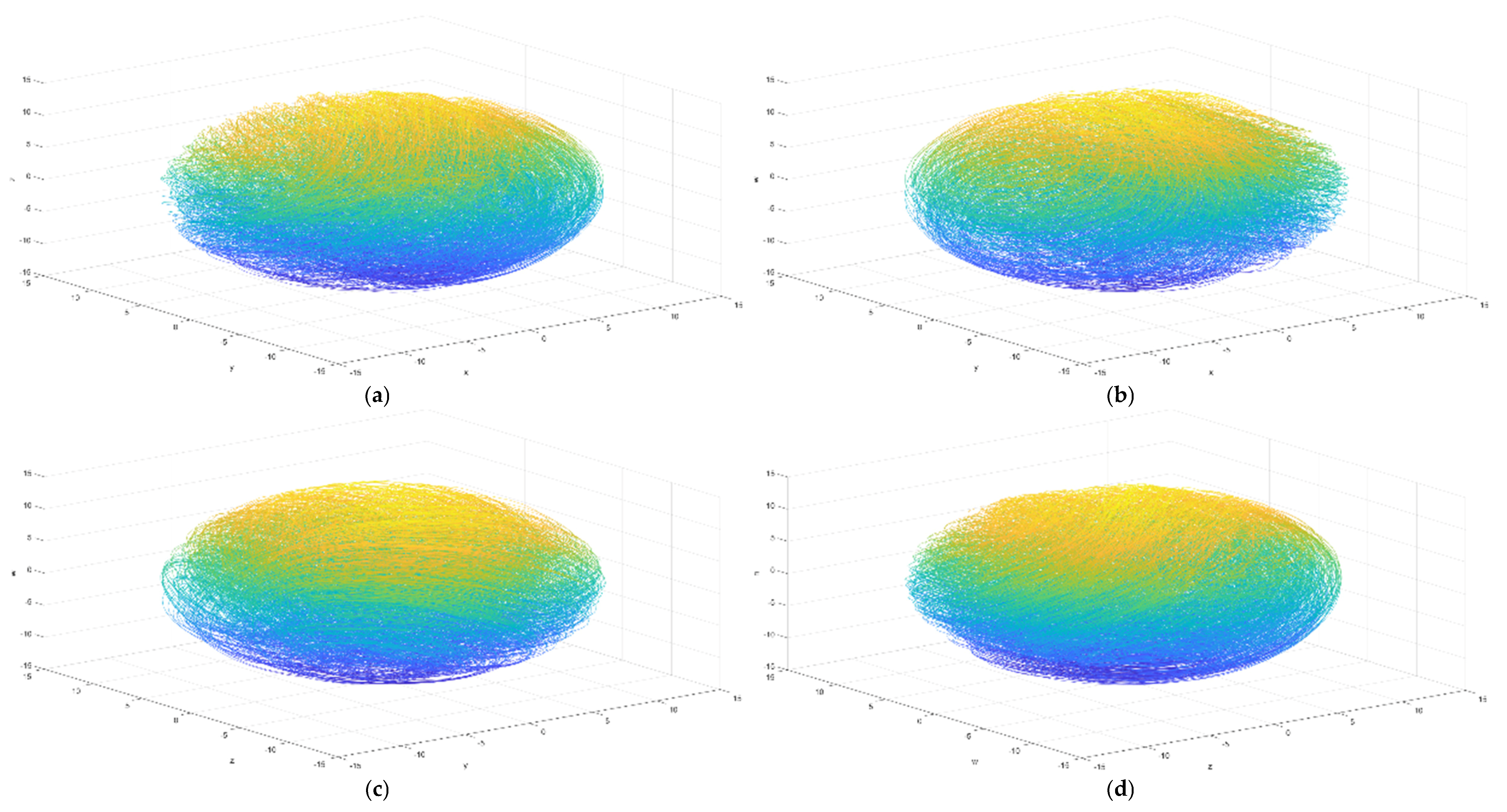
Figure 1.
The chaotic attractor of 5D Harmiltonian conservative hyper-chaotic system: (a) X-Y phase space; (b) Y-Z phase space; (c) Z-W phase space; (d) W-N phase space; (e) X-Y-Z phase space; (f) X-Y-W phase space; (g) Y-Z-W phase space; (h) Z-W-N phase space.
Figure 1.
The chaotic attractor of 5D Harmiltonian conservative hyper-chaotic system: (a) X-Y phase space; (b) Y-Z phase space; (c) Z-W phase space; (d) W-N phase space; (e) X-Y-Z phase space; (f) X-Y-W phase space; (g) Y-Z-W phase space; (h) Z-W-N phase space.
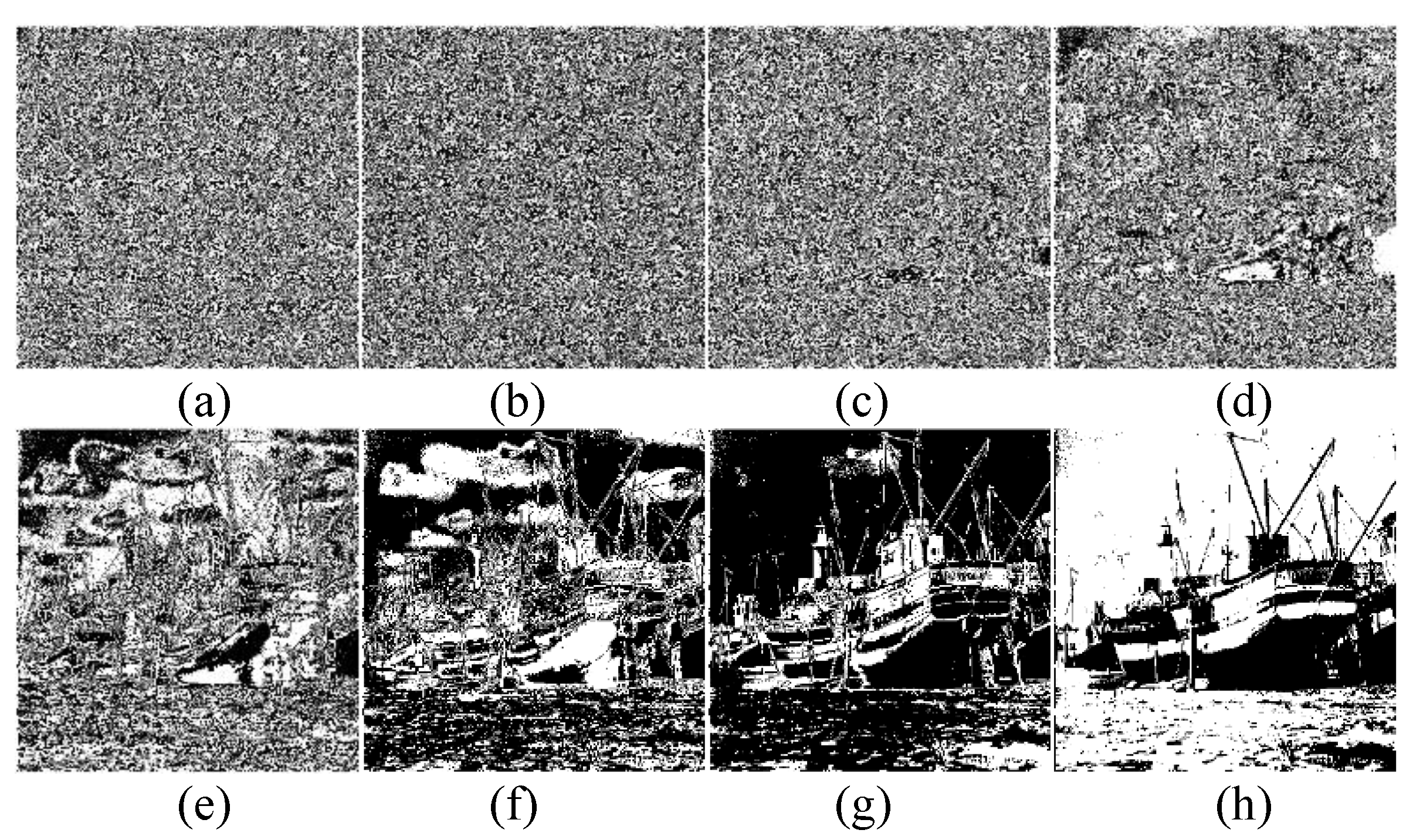
Figure 2.
Bit-plane decomposition result of Image Boat. (a–d): low-bit-planes; (e–h): high-bit-planes.
Figure 2.
Bit-plane decomposition result of Image Boat. (a–d): low-bit-planes; (e–h): high-bit-planes.
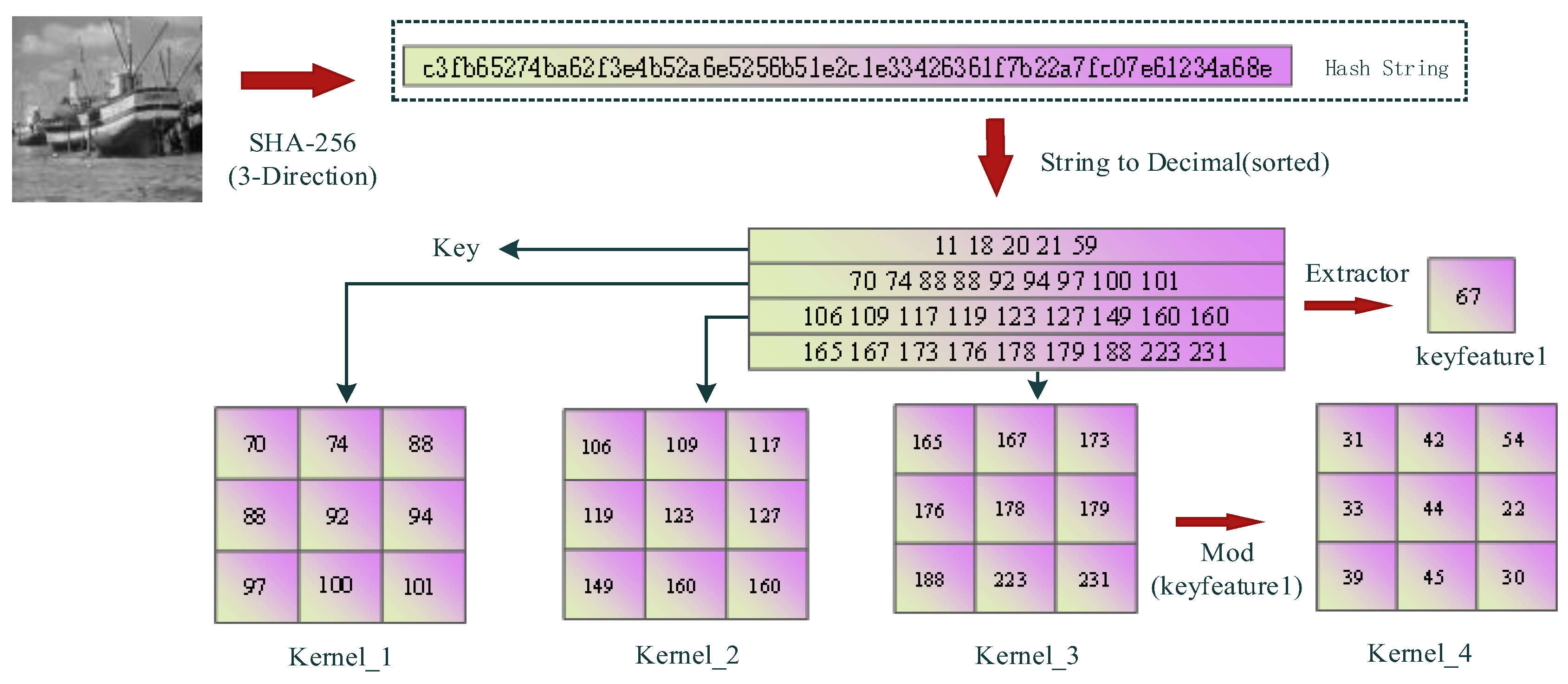
Figure 3.
Plaintext-related sequence generator.
Figure 3.
Plaintext-related sequence generator.
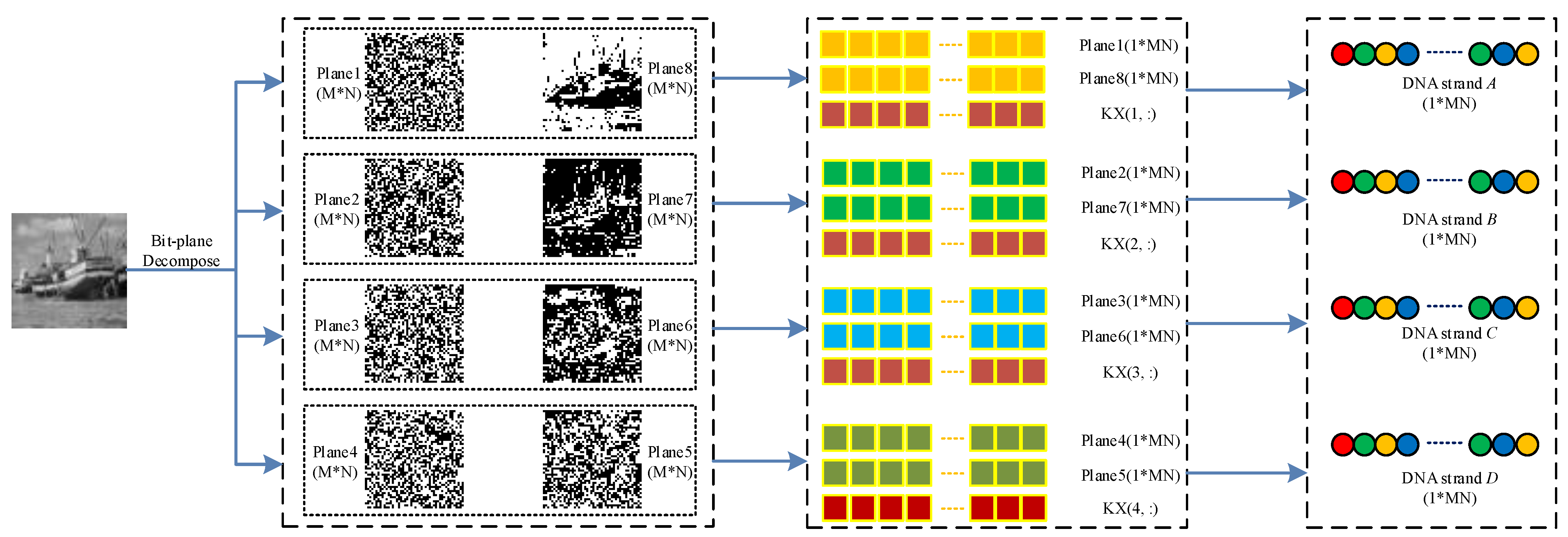
Figure 4.
The flowchart of DNA strand generation.
Figure 4.
The flowchart of DNA strand generation.
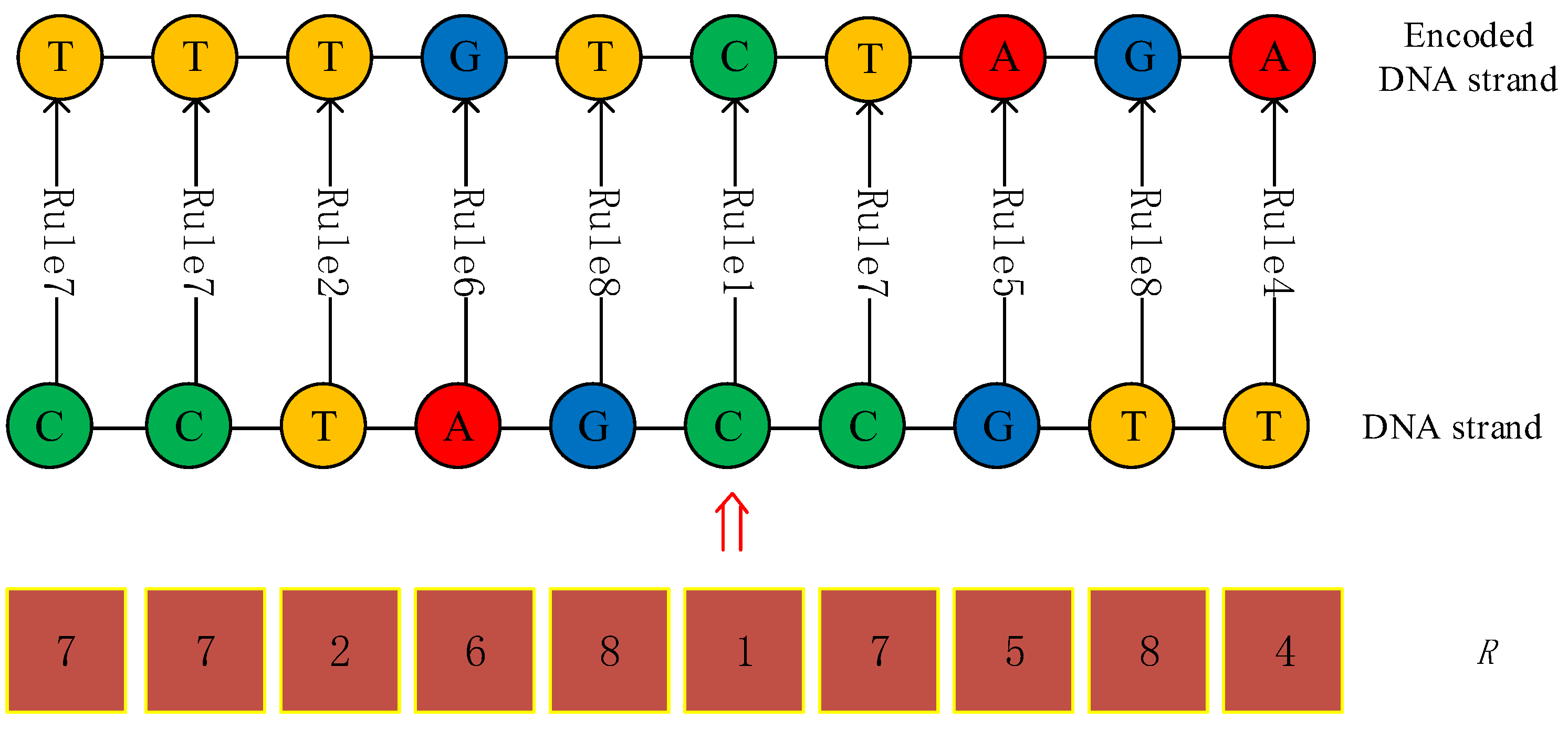
Figure 5.
An example of DNA strand generation process.
Figure 5.
An example of DNA strand generation process.
Figure 6.
An example of DNA strand permutation process.
Figure 6.
An example of DNA strand permutation process.
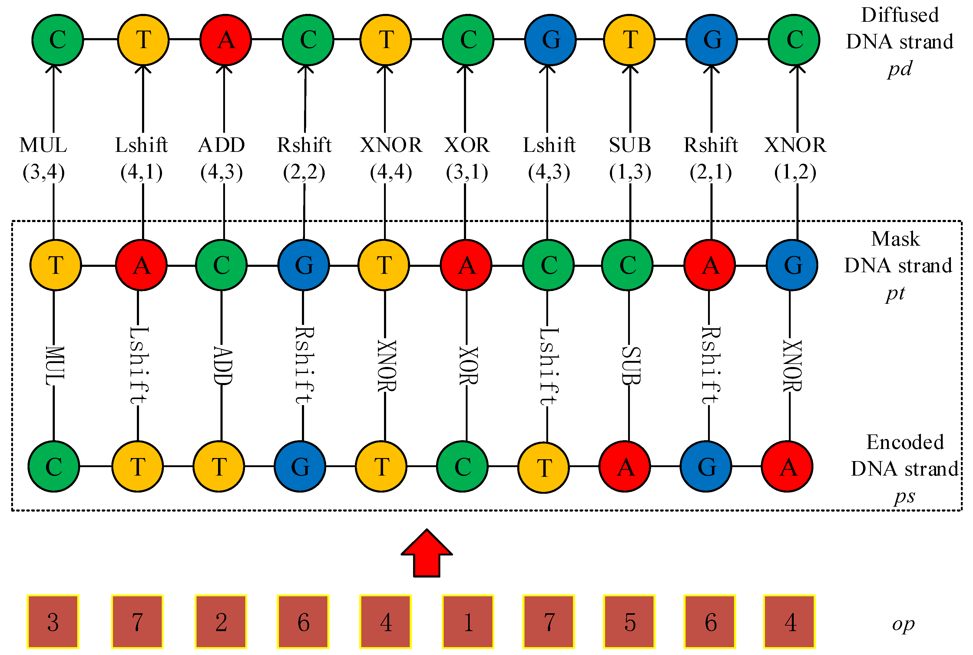
Figure 7.
An example of DNA strand diffusion process.
Figure 7.
An example of DNA strand diffusion process.
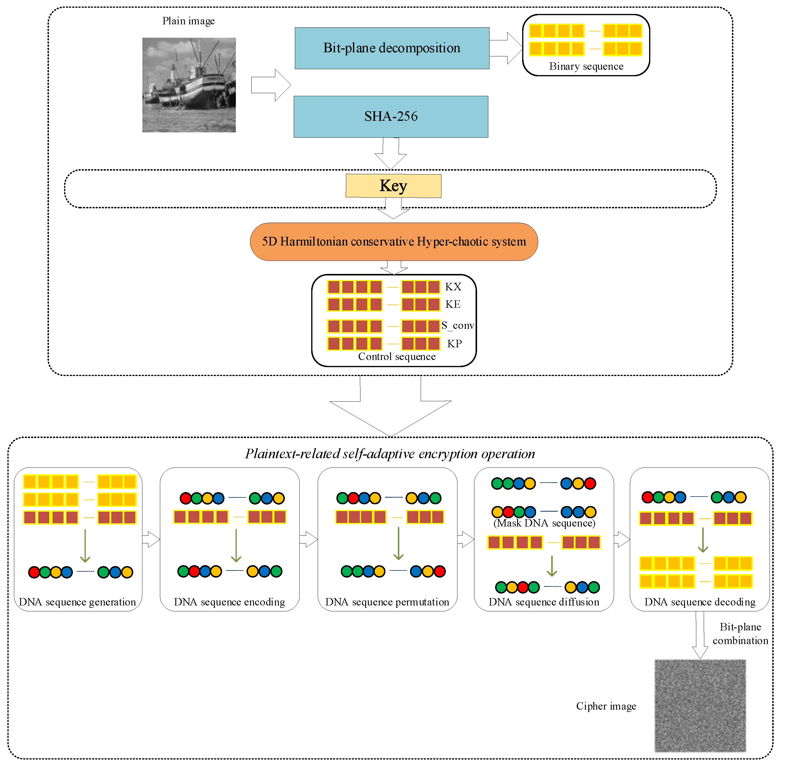
Figure 8.
Image encryption process.
Figure 8.
Image encryption process.
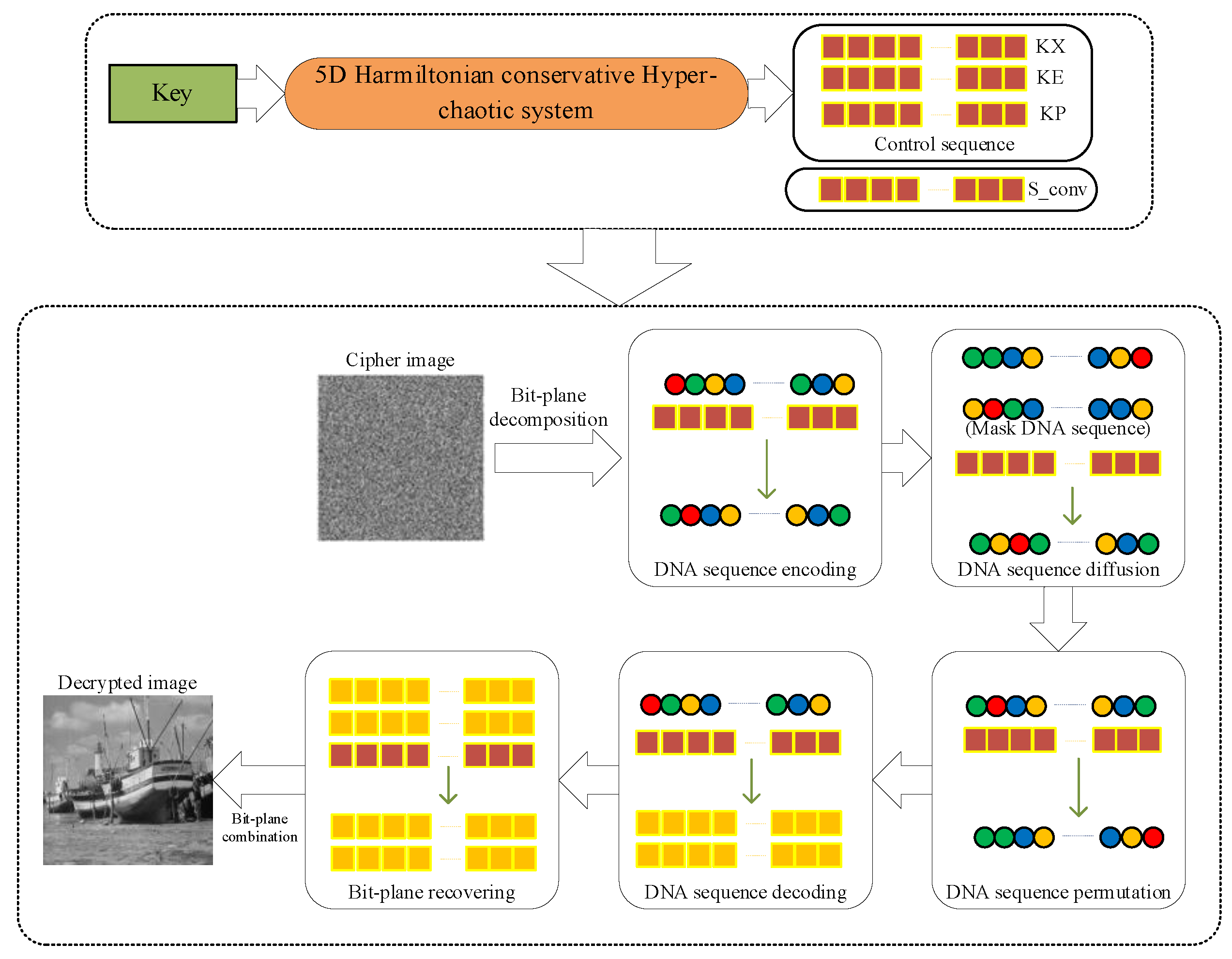
Figure 9.
Image decryption process.
Figure 9.
Image decryption process.
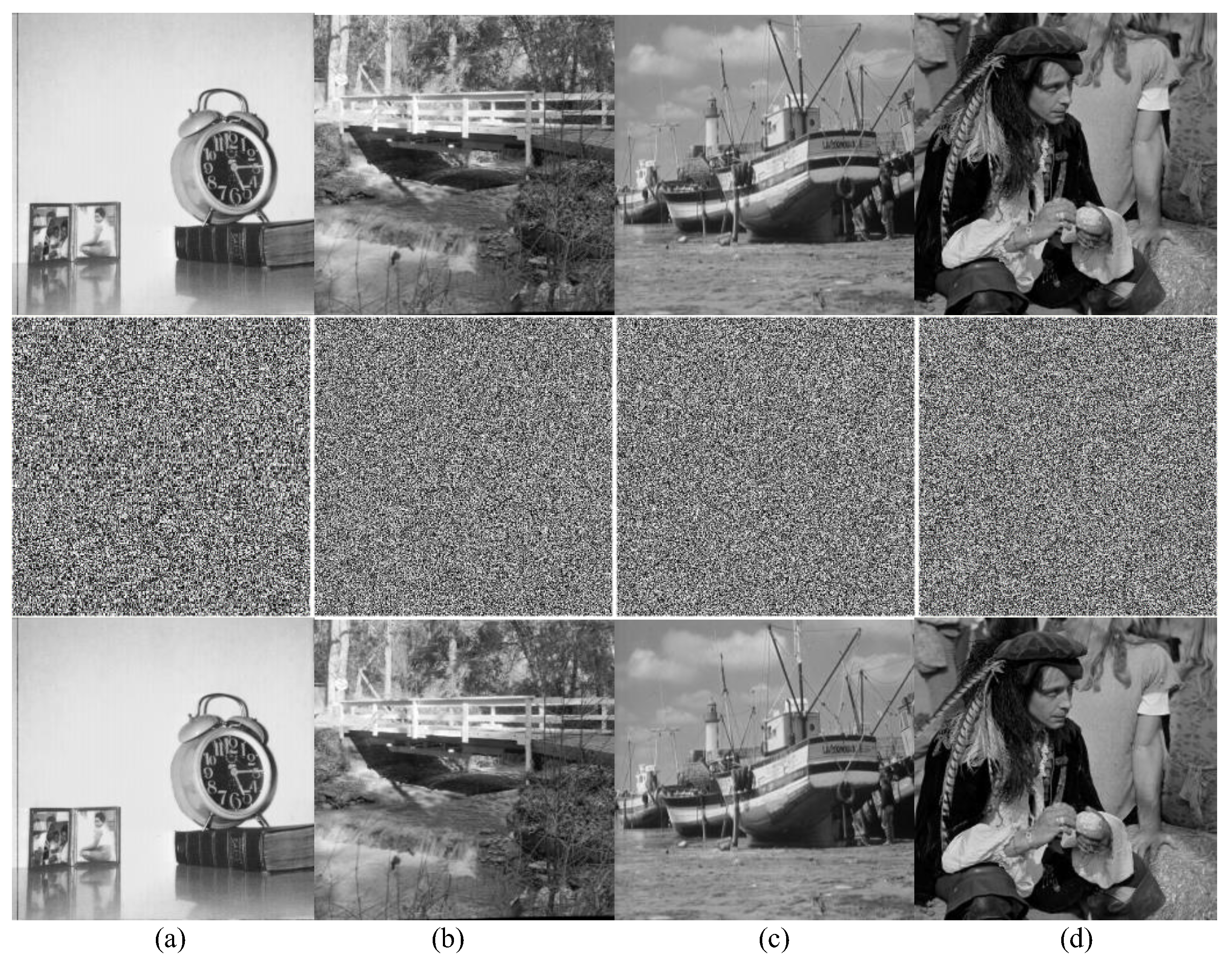
Figure 10.
Encryption results of Group 1: (a) clock (256 × 256); (b) bridge (512 × 512); (c) boat (512 × 512); (d) male (1024 × 1024). First line: plain images; second line: encrypted images; third line: decrypted images.
Figure 10.
Encryption results of Group 1: (a) clock (256 × 256); (b) bridge (512 × 512); (c) boat (512 × 512); (d) male (1024 × 1024). First line: plain images; second line: encrypted images; third line: decrypted images.
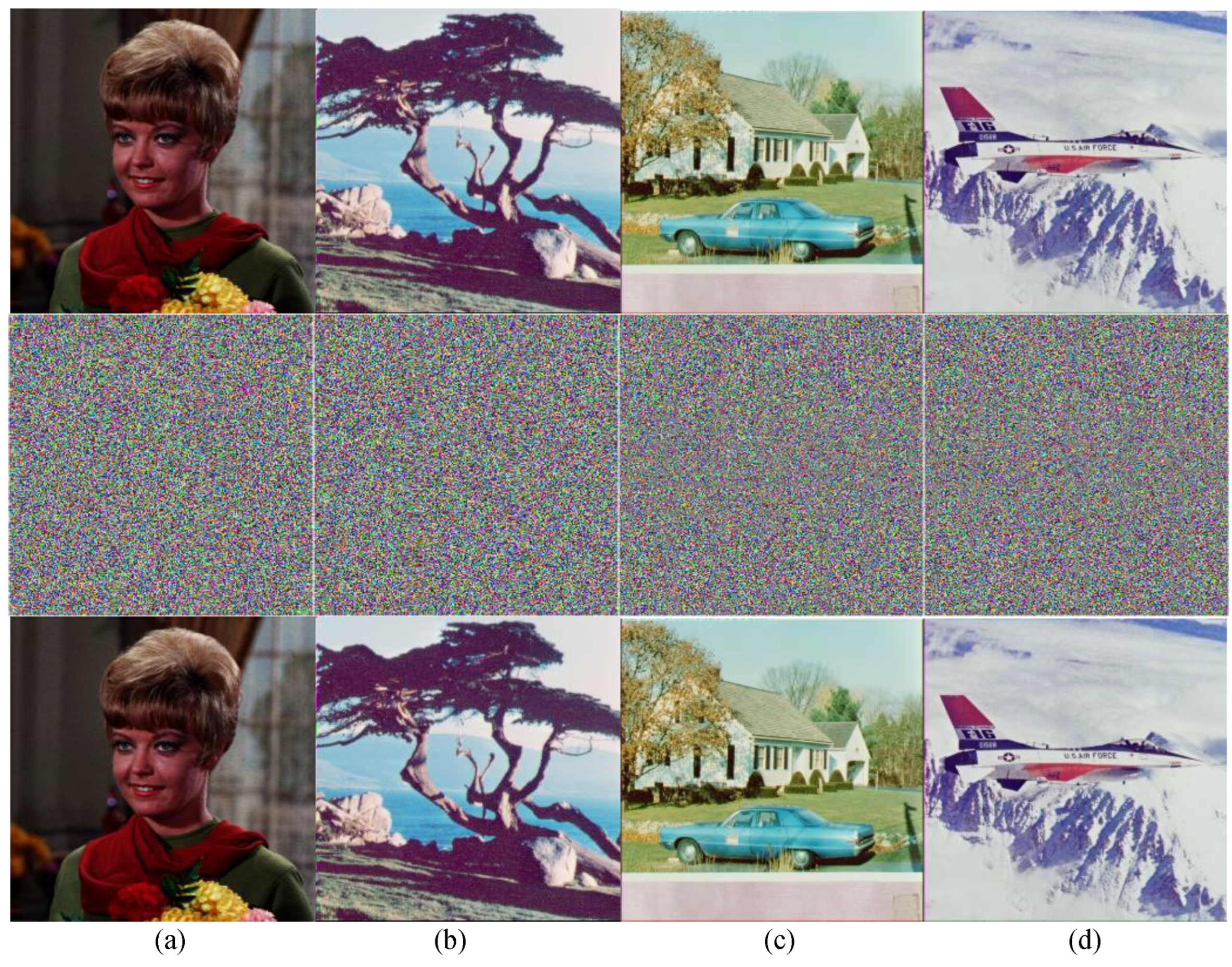
Figure 11.
Encryption results of Group 2: (a) female (256 × 256 × 3); (b) pine (256 × 256 × 3); (c) house (512 × 512 × 3); (d) fighter (512 × 512 × 3). First line: plain images; second line: encrypted images; third line: decrypted images.
Figure 11.
Encryption results of Group 2: (a) female (256 × 256 × 3); (b) pine (256 × 256 × 3); (c) house (512 × 512 × 3); (d) fighter (512 × 512 × 3). First line: plain images; second line: encrypted images; third line: decrypted images.
Figure 12.
Key sensitivity experiment: (a) cipher image “Boat”; (b–f) use incorrect key to decrypt: , , , , ; (g) use correct key to decrypt.
Figure 12.
Key sensitivity experiment: (a) cipher image “Boat”; (b–f) use incorrect key to decrypt: , , , , ; (g) use correct key to decrypt.
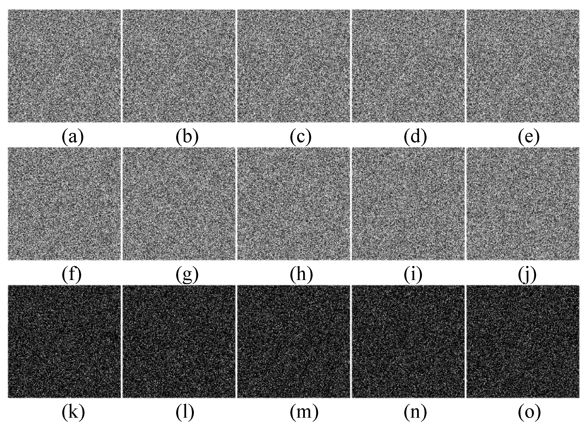
Figure 13.
Cipher image difference (“Boat”). (a–e): cipher image using , , , , ; (f–j): cipher image using , , , , ; (k–o): difference between cipher images (a–e) and cipher images (f–j).
Figure 13.
Cipher image difference (“Boat”). (a–e): cipher image using , , , , ; (f–j): cipher image using , , , , ; (k–o): difference between cipher images (a–e) and cipher images (f–j).
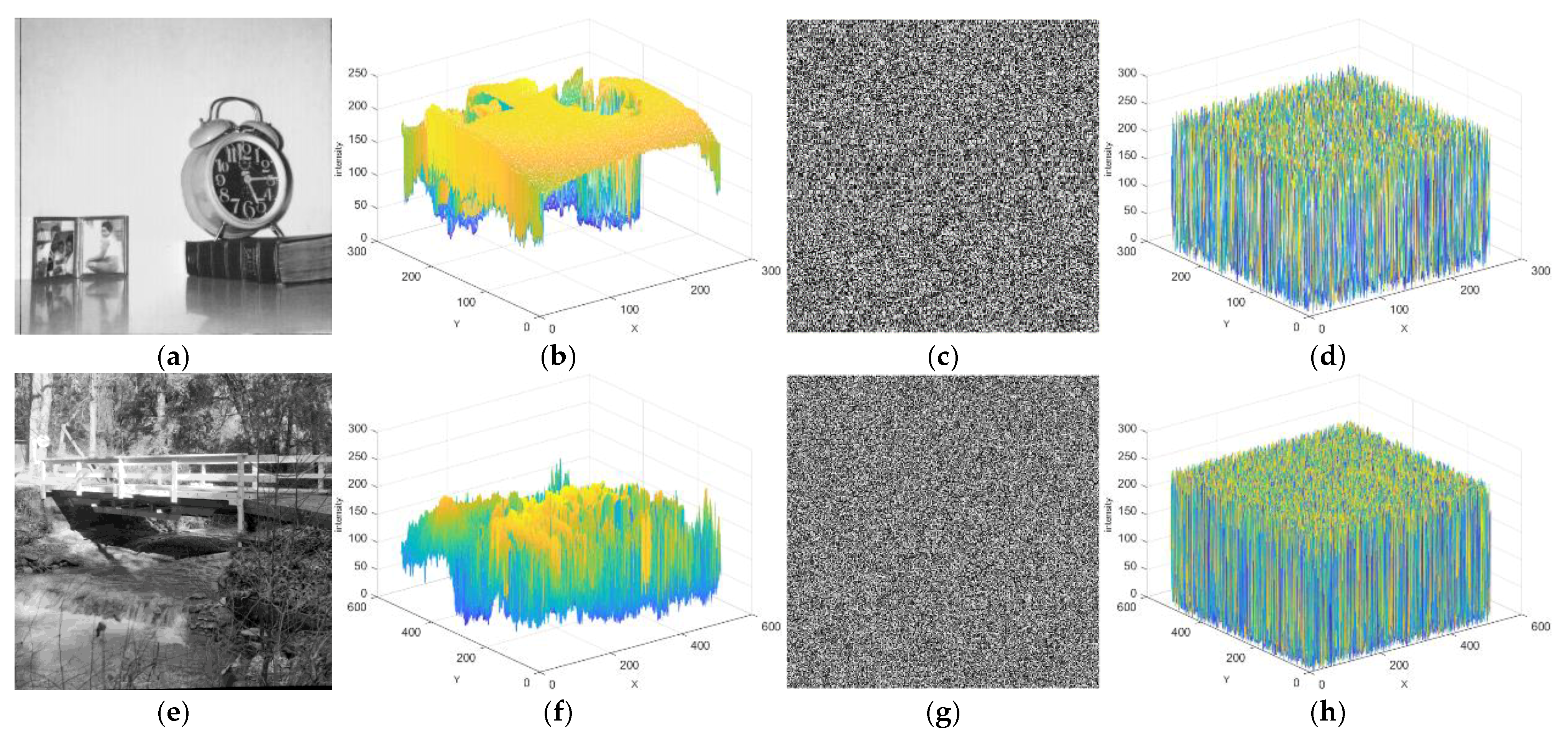
Figure 14.
Image 3D histogram. (a,e,i,m,q,u): plain images; (b,f,j,n,r,v): 3D histograms of plain images; (c,g,k,o,s,w): cipher images; (d,h,l,p,t,x): 3D histograms of cipher images.
Figure 14.
Image 3D histogram. (a,e,i,m,q,u): plain images; (b,f,j,n,r,v): 3D histograms of plain images; (c,g,k,o,s,w): cipher images; (d,h,l,p,t,x): 3D histograms of cipher images.
Figure 15.
Adjacent pixel correlation distribution. (a): plain images; (b): correlation distribution of plain images; (c): corresponding cipher images; (d): correlation distribution of cipher images.
Figure 15.
Adjacent pixel correlation distribution. (a): plain images; (b): correlation distribution of plain images; (c): corresponding cipher images; (d): correlation distribution of cipher images.
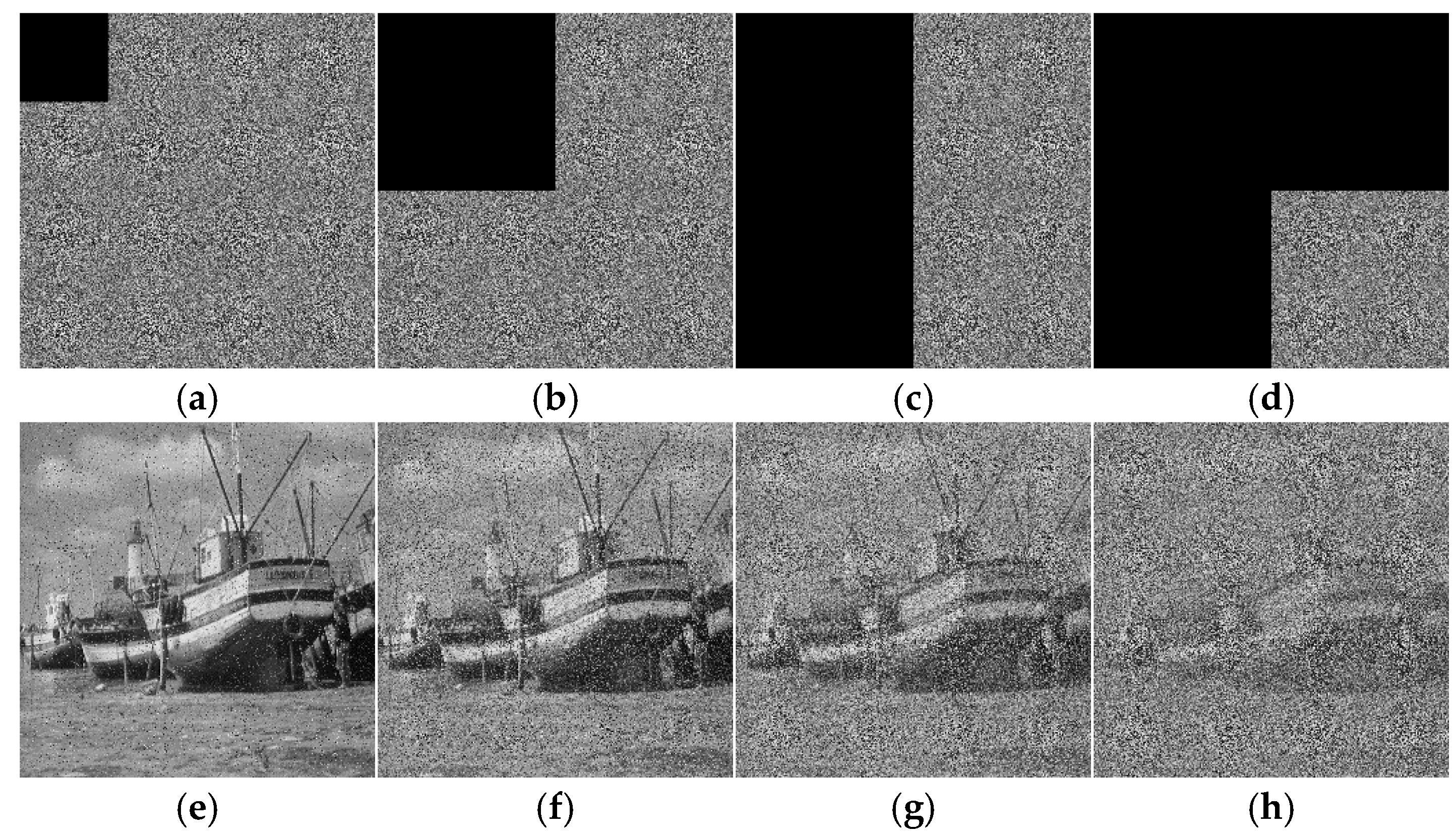
Figure 16.
The results of the cropping attacks: (a–d) cipher image of 1/16, 1/4, 1/2, 3/4 cropping attacks; (e–h) corresponding decrypted image of different cropping attacks.
Figure 16.
The results of the cropping attacks: (a–d) cipher image of 1/16, 1/4, 1/2, 3/4 cropping attacks; (e–h) corresponding decrypted image of different cropping attacks.
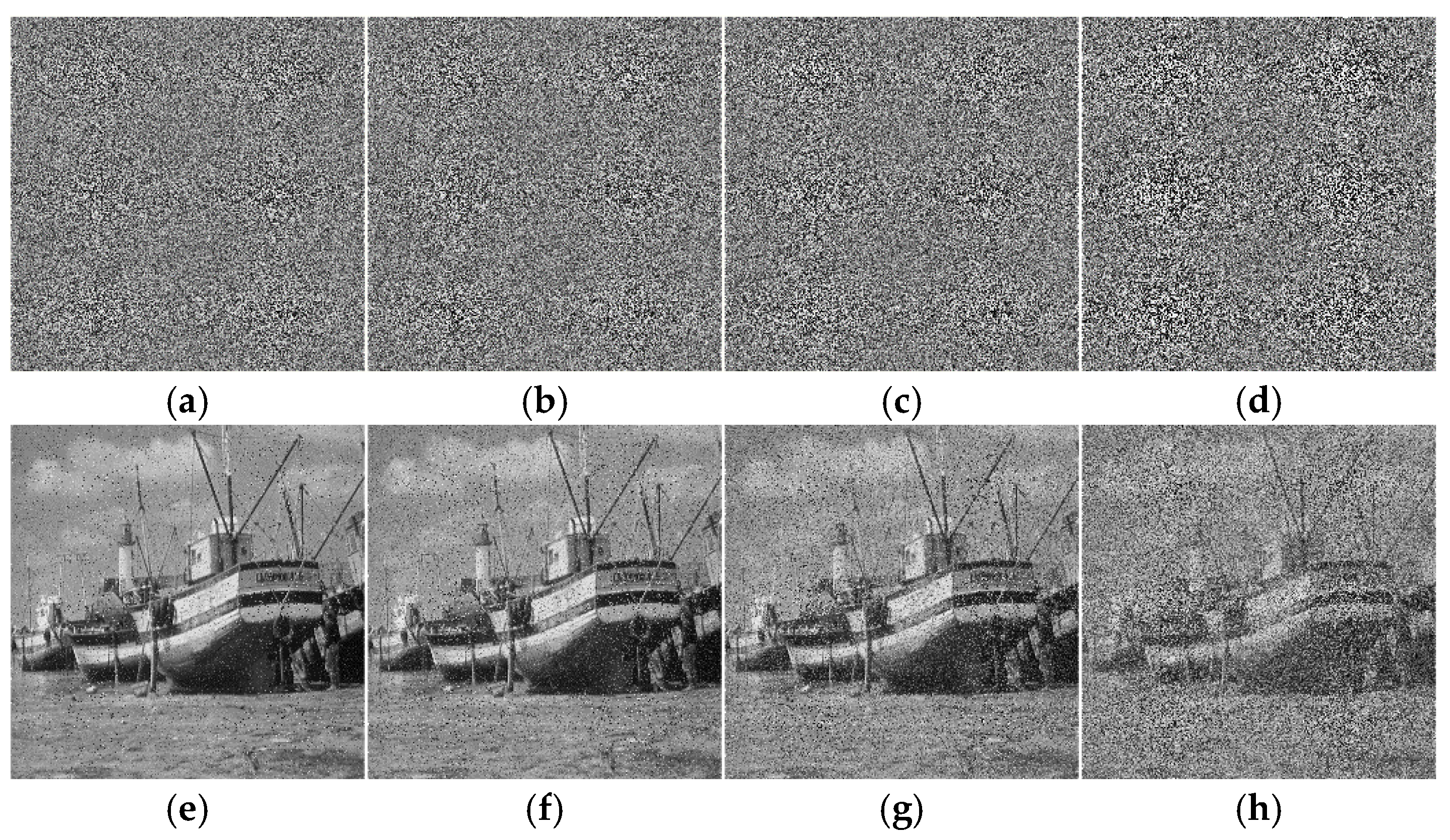
Figure 17.
The results of the noise attacks: (a–d) cipher image of 0.05, 0.1, 0.2, 0.5 noise attacks; (e–h) corresponding decrypted image of different noise attacks.
Figure 17.
The results of the noise attacks: (a–d) cipher image of 0.05, 0.1, 0.2, 0.5 noise attacks; (e–h) corresponding decrypted image of different noise attacks.
Table 1.
The calculation result of proportion of information carried.
Table 1.
The calculation result of proportion of information carried.
| Bit-Planes | 1th | 2th | 3th | 4th | 5th | 6th | 7th | 8th |
|---|
| Proportion (%) | 0.39 | 0.78 | 1.57 | 3.14 | 6.27 | 12.55 | 25.10 | 50.20 |
| 5.88 | 94.12 |
Table 2.
DNA encoding and decoding rules.
Table 2.
DNA encoding and decoding rules.
| Rule | 1 | 2 | 3 | 4 | 5 | 6 | 7 | 8 |
|---|
| 00 | A | A | T | T | G | G | C | C |
| 01 | G | C | G | C | A | T | A | T |
| 10 | C | G | C | G | T | A | T | A |
| 11 | T | T | A | A | C | C | G | G |
Table 3.
DNA arithmetic operations.
Table 3.
DNA arithmetic operations.
| ⊕/⊗/+/− | A | G | C | T |
|---|
| A | A/T/A/A | G/C/G/T | C/G/C/C | T/A/T/G |
| G | G/C/G/G | A/T/C/A | T/A/T/T | C/G/A/C |
| C | C/G/C/C | T/A/T/G | A/T/A/A | G/C/G/T |
| T | T/A/T/T | C/G/A/C | G/C/G/G | A/T/C/A |
Table 4.
Key space comparison.
Table 4.
Key space comparison.
| | Proposed | [24] | [23] | [25] | [26] | [19] | [27] |
|---|
| Key space | | | | | | | |
Table 5.
Difference between two cipher images.
Table 5.
Difference between two cipher images.
| Cipher Images | Key | Difference (%) |
|---|
| Figure 13a | Figure 13f | | | 99.46 |
| Figure 13b | Figure 13g | | | 99.60 |
| Figure 13c | Figure 13h | | | 99.62 |
| Figure 13d | Figure 13i | | | 99.50 |
| Figure 13e | Figure 13j | | | 99.67 |
Table 6.
Variances of histograms.
Table 6.
Variances of histograms.
| Image | Clock | Bridge | Boat | Male |
|---|
| Plain | 283,167.686 | 4,761,071.325 | 1,541,901.804 | 11,393,958.533 |
| Cipher | 332.463 | 902.086 | 953.765 | 3818.102 |
Table 7.
Variances of histograms with different keys.
Table 7.
Variances of histograms with different keys.
| Cipher Image | Key | | | | | | | | | | |
|---|
| Bridge | 902.086 | 885.467 | 974.031 | 986.126 | 887.224 | 850.361 | 965.992 | 928.494 | 869.106 | 940.251 | 961.851 |
| Boat | 953.765 | 1026.784 | 874.314 | 968.047 | 975.937 | 1022.620 | 982.737 | 973.702 | 1024.275 | 908.267 | 1027.388 |
| Couple | 1036.478 | 1004.761 | 945.247 | 1001.655 | 1088.980 | 1031.922 | 994.800 | 1078.549 | 1136.659 | 1055.271 | 1008.400 |
| Tank | 1003.639 | 1043.333 | 1083.906 | 1110.706 | 1044.965 | 988.329 | 1053.325 | 1009.741 | 1034.439 | 928.816 | 1035.663 |
| Average | 973.992 | 990.086 | 969.375 | 1016.634 | 999.276 | 973.308 | 999.214 | 997.622 | 1016.120 | 958.151 | 1008.325 |
Table 8.
Variance change rate of different keys.
Table 8.
Variance change rate of different keys.
| Cipher Image | | | | | | | | | | |
|---|
| Bridge | 1.84% | 7.98% | 9.32% | 1.65% | 5.73% | 7.08% | 2.93% | 3.66% | 4.23% | 6.63% |
| Boat | 7.66% | 8.33% | 1.50% | 2.32% | 7.22% | 3.04% | 2.09% | 7.39% | 4.77% | 7.72% |
| Couple | 3.06% | 8.80% | 3.36% | 5.07% | 0.44% | 4.02% | 4.06% | 9.67% | 1.81% | 2.71% |
| Tank | 3.96% | 8.00% | 10.67% | 4.12% | 1.53% | 4.95% | 0.61% | 3.07% | 7.46% | 3.19% |
| Average | 1.65% | 0.47% | 4.38% | 2.60% | 0.07% | 2.59% | 2.43% | 4.33% | 1.63% | 3.53% |
Table 9.
Comparison of histogram variances.
Table 9.
Comparison of histogram variances.
| Methods | Lena | Barbara | Peppers | Male |
|---|
| Proposed | 982.808 | 986.345 | 959.671 | 3818.102 |
| [24] | 993.570 | 1042.672 | 967.367 | 4020.578 |
| [28] | 1047.655 | 941.168 | - | - |
| [29] | 5335.83 | 5013.88 | - | - |
Table 10.
Correlation coefficients of different images.
Table 10.
Correlation coefficients of different images.
| Images | Plain Image | Cipher Image |
|---|
| H | V | D | H | V | D |
|---|
| Clock | 0.95632 | 0.97219 | 0.93790 | 0.00383 | −0.00007 | 0.00606 |
| Bridge | 0.94046 | 0.91962 | 0.89272 | −0.00496 | −0.00299 | 0.00538 |
| Boat | 0.93446 | 0.97153 | 0.92095 | 0.00660 | −0.00848 | −0.00036 |
| Male | 0.97944 | 0.97910 | 0.96400 | 0.00154 | −0.00418 | 0.00716 |
| Couple | 0.93419 | 0.88103 | 0.84819 | 0.00762 | −0.00273 | 0.00162 |
| Tank | 0.94344 | 0.93047 | 0.89739 | 0.00304 | −0.00660 | 0.00528 |
| Lena | 0.96774 | 0.98533 | 0.95554 | −0.00109 | −0.00039 | 0.00007 |
| Peppers | 0.97200 | 0.97781 | 0.95525 | 0.00027 | −0.00042 | −0.00076 |
Table 11.
Correlation coefficients comparison of Peppers image.
Table 11.
Correlation coefficients comparison of Peppers image.
| Algorithms | Cipher Image |
|---|
| H | V | D |
|---|
| Proposed | 0.00027 | −0.00042 | −0.00076 |
| [24] | −0.0002 | −0.0029 | −0.0061 |
| [21] | 0.0089 | −0.0037 | −0.0042 |
| [30] | 0.0139 | 0.0054 | 0.0153 |
| [31] | −0.0013 | 0.0019 | 0.0009 |
Table 12.
Correlation coefficients comparison of Lena image.
Table 12.
Correlation coefficients comparison of Lena image.
| Algorithms | Cipher Image |
|---|
| H | V | D |
|---|
| Proposed | −0.00109 | −0.00039 | 0.00007 |
| [32] | −0.0020 | −0.0065 | 0.0087 |
| [33] | −0.0017 | −0.0009 | −0.0019 |
| [34] | −0.0239 | −0.0033 | 0.0046 |
| [35] | 0.0115 | 0.0193 | 0.0234 |
| [36] | 0.0085 | 0.0054 | 0.0049 |
| [15] | 0.0004 | −0.0033 | −0.0070 |
Table 13.
Comparison results of test.
Table 13.
Comparison results of test.
| Algorithms | Images | Test |
|---|
| Plain Image | Cipher Image |
|---|
| Proposed | Clock | 282,062 | 244.914 |
| Couple | 298,865 | 247.254 |
| Peppers | 120,166 | 243.246 |
| Male | 709,341 | 194.333 |
| Lena | 158,349 | 185.645 |
| Boat | 383,970 | 255.762 |
| Bridge | 1,185,618 | 210.523 |
| Tank | 2,025,900 | 249.018 |
| Baboon | 187,357 | 254.293 |
| [21] | Peppers | - | 264.77 |
| [30] | Peppers | - | 287.22 |
| [31] | Peppers | - | 271.90 |
| [24] | Peppers | - | 253.08 |
| [28] | Peppers | - | 247.56 |
| [15] | Lena | - | 218 |
| [32] | Lena | - | 229 |
| [37] | Lena | - | 230 |
| [38] | Lena | - | 230 |
| [39] | Lena | - | 285 |
Table 14.
Comparison results of information entropy.
Table 14.
Comparison results of information entropy.
| Algorithms | Images | Information Entropy |
|---|
| Plain Image | Cipher Image |
|---|
| Proposed | Clock | 6.7057 | 7.9973 |
| Couple | 7.2010 | 7.9993 |
| Peppers | 7.5937 | 7.9994 |
| Male | 7.5237 | 7.9999 |
| Lena | 7.4451 | 7.9995 |
| Boat | 7.1914 | 7.9993 |
| Bridge | 5.7056 | 7.9994 |
| Tank | 5.4957 | 7.9993 |
| Baboon | 7.3583 | 7.9993 |
| [15] | Lena | - | 7.9971 |
| [25] | Lena | - | 7.9971 |
| [40] | Lena | - | 7.9994 |
| [41] | Lena | - | 7.9993 |
| [28] | Lena | - | 7.9993 |
| [24] | Peppers | - | 7.9993 |
| [28] | Peppers | - | 7.9993 |
| [15] | Peppers | - | 7.9993 |
| [19] | Peppers | - | 7.9981 |
| [25] | Peppers | - | 7.9971 |
Table 15.
MSE and PSNR result.
Table 15.
MSE and PSNR result.
| Algorithms | Image | MSE | PSNR |
|---|
| Cipher | Decrypted |
|---|
| proposed | Clock | 12,133.9 | 7.2791 | ∞ |
| Couple | 7090.1 | 9.6085 | ∞ |
| Peppers | 9428.4 | 8.3794 | ∞ |
| Male | 10,288.3 | 7.9977 | ∞ |
| Lena | 7754.2 | 9.2296 | ∞ |
| Boat | 7628.4 | 9.3065 | ∞ |
| Bridge | 8648.3 | 8.7615 | ∞ |
| Tank | 6213.1 | 10.1977 | ∞ |
| Baboon | 7285.1 | 9.5065 | ∞ |
| [24] | Peppers | 9267.0 | 8.4614 | - |
| [24] | Male | 10,294.6 | 8.0047 | - |
| [24] | Couple | 7089.2 | 9.6248 | |
| [22] | Peppers | 9311.7 | 8.4405 | - |
| [22] | Lena | 7752.6 | 9.2363 | - |
Table 16.
NIST test.
| Test Items | Key: KM | Key: KE | Key: KP | Key: KX |
|---|
| Frequency test | 0.991468 | 0.922325 | 0.863341 | 0.913568 |
| Frequency test within a block | 0.350485 | 0.350485 | 0.426843 | 0.269864 |
| Cumulative sums test | 0.739918 | 0.534146 | 0.634896 | 0.648576 |
| Discrete fourier transform test | 0.834308 | 0.622325 | 0.725563 | 0.268573 |
| Test for the longest run of ones in a block | 0.911413 | 0.805189 | 0.415371 | 0.897631 |
| Random excursions variant test (x = 1) | 0.184287 | 0.911413 | 0.185632 | 0.213547 |
| Runs test | 0.637119 | 0.017912 | 0.223575 | 0.168573 |
| Non-overlapping template matching test (m = 9) | 0.995253 | 0.739918 | 0.279563 | 0.245982 |
| Overlapping template matching test (m = 9) | 0.929703 | 0.916905 | 0.958254 | 0.987024 |
| Maurer’s “Universal statistical” test | 0.637683 | 0.720774 | 0.547635 | 0.635794 |
| Approximate entropy test | 0.231344 | 0.658603 | 0.446578 | 0.324359 |
| Random excursions test (x = 1) | 0.919708 | 0.773446 | 0.354783 | 0.738972 |
| Serial test | 0.833230 | 0.630451 | 0.885763 | 0.824629 |
| Linear complexity test | 0.888998 | 0.213309 | 0.514790 | 0.883671 |
| Binary matrix rank test | 0.350485 | 0.956353 | 0.965873 | 0.896542 |
Table 17.
NPCR and UACI.
| Algorithms | Image | NPCR (%) | UACI (%) |
|---|
| proposed | Clock | 99.6124 | 33.4044 |
| Couple | 99.6326 | 33.4924 |
| Peppers | 99.6101 | 33.4626 |
| Male | 99.6132 | 33.4302 |
| Lena | 99.6216 | 33.4556 |
| Boat | 99.6159 | 33.4404 |
| Bridge | 99.6197 | 33.4570 |
| Tank | 99.5804 | 33.4169 |
| Baboon | 99.6143 | 33.4834 |
| [15] | Lena | 99.6246 | 33.4115 |
| [32] | Lena | 99.6063 | 33.4477 |
| [36] | Lena | 99.636 | 33.465 |
| [42] | Lena | 99.6096 | 33.4645 |
| [41] | Lena | 99.65 | 33.61 |
| [24] | Peppers | 99.6101 | 33.4689 |
| [30] | Peppers | 99.6086 | 33.4398 |
| [43] | Peppers | 99.6068 | 33.4332 |
| [44] | Peppers | 99.6083 | 29.6188 |
| [15] | Peppers | 99.5922 | 33.3953 |
Table 18.
EQ value of different images.
Table 18.
EQ value of different images.
| Image | Clock | Couple | Peppers | Male | Lena | Boat | Bridge | Tank | Baboon | Airplane |
|---|
| EQ value | 243.180 | 868.469 | 666.336 | 2325.789 | 664.695 | 866.664 | 1560.523 | 1483.602 | 775.031 | 1083.617 |
Table 19.
The comparison of EQ value.
Table 19.
The comparison of EQ value.
| Algorithms | Clock | Peppers | Airplane |
|---|
| Proposed | 243.180 | 666.336 | 1083 |
| [24] | 242 | 608 | 1083 |
| [45] | 244 | 156 | 303 |
| [46] | 243 | 156 | 302 |
| [47] | 243 | 158 | 300 |
Table 20.
MD values of different images.
Table 20.
MD values of different images.
| Image | Clock | Couple | Peppers | Male | Lena | Boat | Bridge | Tank | Baboon | Girl | Cameraman |
|---|
| MD value | 62,006.5 | 221,745.5 | 144,003.5 | 580,419 | 169,140.5 | 220,897.5 | 398,970.5 | 378,793.5 | 197,379 | 59,322.5 | 64,374 |
Table 21.
Comparison results of MD values.
Table 21.
Comparison results of MD values.
| Algorithms | Cameraman | Baboon | Girl |
|---|
| Proposed | 64,374 | 207,379 | 59,322.5 |
| [24] | 255,613 | 201,300 | 58,741 |
| [46] | 63,920 | 46,540 | 49,588 |
| [48] | 49,129 | 17,652 | 48,639 |
| [49] | 38,912 | 55,129 | 39,187 |
Table 22.
Comparison results of execution time analysis.
Table 22.
Comparison results of execution time analysis.
| Algorithm | Image Size | Encryption Time | Decryption Time | Platform & Hardware |
|---|
| Proposed | 256 × 256 | 0.3280 | 0.3944 | MATLAB R2022a, CPU i7&2.80GHz, 8G RAM |
| 512 × 512 | 1.3650 | 1.5832 |
| 1024 × 1024 | 5.3446 | 6.6094 |
| [22] | 256 × 256 | 0.380 | 0.463 | MATLAB R2020a, CPU i5&2.80GHz, 8G RAM |
| 512 × 512 | 1.431 | 1.633 |
| 1024 × 1024 | 5.719 | 6.759 |
| [50] | 512 × 512 | 1.6455 | - | MATLAB R2013a, CPU i3&2.4 GHz, 4G RAM |
| [51] | 23.142 | - | MATLAB R2018b, CPU i7&3.4 GHz, 8G RAM |
| [52] | 6.8816 | - | MATLAB R2017a, CPU i5&2.3 GHz, 8G RAM |
| [53] | 6.0752 | - | MATLAB R2017a, CPU i5&2.8 GHz, 8G RAM |
Table 23.
Execution time of every encryption step.
Table 23.
Execution time of every encryption step.
| Steps | Time (/s) | Percentage |
|---|
| Hyper-chaotic sequence generation | 0.8012 | 59% |
| Convolution sequence generation | 0.0178 | 1% |
| Bit-plane decomposition | 0.0332 | 2% |
| DNA strand generation | 0.0677 | 5% |
| DNA strand encoding | 0.0518 | 4% |
| DNA strand permutation | 0.0603 | 4% |
| DNA strand diffusion | 0.0314 | 2% |
| DNA strand decoding | 0.2841 | 21% |
| Bit-plane combination |
| Other | 0.0175 | 1% |
| Total | 1.3650 | 100% |


