Nonequilibrium Molecular Velocity Distribution Functions Predicted by Macroscopic Gas Dynamic Models ^†

Abstract

In the present study, abilities of various macroscopic models (Navier–Stokes–Fourier, Burnett, original and regularized Grad’s 13-moment equations) in predicting the nonequilibrium molecular velocity distribution are examined. The results of the local distribution function reconstruction from flow macroparameters for the models considered are compared with each other and with the reference solution. Two different flows are considered: normal shock wave and stationary regular reflection of oblique shock waves. The Direct Simulation Monte Carlo method is used to obtain the reference solution and the flow macroparameters required for the distribution function reconstruction. All models under consideration predict the distribution function in the upstream low-density region rather poorly, with strong oscillations and unphysical negative values (especially regularized Grad’s 13-moment equations). In the high-density downstream region, the shape of the reference distribution is close to equilibrium, and all macroscopic models predict it rather accurately.

1. Introduction

The kinetic Boltzmann equation is the central mathematical model of rarefied gas dynamics and kinetic theory of gases [1]. Rarefied flows of an ideal gas can be accurately simulated by solving the Boltzmann equation directly [2,3] or by the Direct Simulation Monte Carlo (DSMC) method [4,5]. Usually, such an approach to numerical modeling of gas flows is called `kinetic’. The sought solution of the equation is the molecular velocity distribution function (phase density). All local gas flow macroparameters at a point can be obtained as moments of the distribution function by averaging the molecular properties (functions of velocity) over the velocity space.

When the local mean free path of molecules is small in comparison with the length scale of interest, the kinetic approach is computationally expensive [6]. On the other hand, the deviation from the equilibrium for such flows can be considered as small. The `continuum’ approach based on various macroscopic gas dynamics models can be applied for such near-continuum flows with much lower computational requirements than the kinetic approach [7,8]. These models describe the flow with a finite number of macroparameters and are constructed in order to approximate the Boltzmann equation solution in near-equilibrium conditions [7,9].

Several methods are employed to derive macroscopic models. The Chapman–Enskog method allows for obtaining the Euler, Navier–Stokes–Fourier (NSF), Burnett, super-Burnett equations directly from the Boltzmann kinetic equation [1,7,9,10,11]. Various systems of moment equations can be obtained with Grad’s method [12]. Systems of regularized moment equations can be obtained using the order of magnitude method [7]. These macroscopic models provide satisfactory agreement to the Boltzmann equation solutions in various problems of rarefied gas dynamics, especially for near-continuum flows, in terms of spatial distributions of macroparameters (see, e.g., Refs. [8,13,14,15,16]).

It is important to note that the above-mentioned models are based on particular assumptions about how the local nonequilibrium velocity distribution function depends on the local gas dynamic macroparameters (such as temperature and pressure) [11,17,18,19] and, in some cases, their gradients. This means that one can reconstruct the velocity distribution function for each model using the flow fields of macroparameters. It might be of substantial interest to compare these approximations of the nonequilibrium velocity distribution function provided by the macroscopic models to the distribution function obtained by accurately solving the Boltzmann equation.

The goal of the present study is to perform such a comparison for a hierarchy of the macroscopic models under conditions of significant thermal nonequilibrium. Reconstructions of the velocity distribution functions are performed with the macroparameter flow fields obtained by the DSMC method, and the DSMC velocity distribution function is considered as a benchmark Boltzmann equation solution. Two problems are chosen for comparisons: the one-dimensional classical problem of the normal shock wave structure and the two-dimensional problem of stationary regular reflection of an oblique shock wave. Both problems share the following important features: first, at high flow Mach numbers, the degree of flow nonequilibrium is substantial; second, the only length scale of the flow is the molecular mean free path, so the analysis is applicable for any degree of rarefaction, even for the continuum flow regime [20]. The Euler, NSF, Burnett, original Grad’s 13-moment (G13), and regularized 13-moment (R13) approximations of the velocity distribution function are examined in this paper. The velocity distribution functions for the macroscopic models considered are presented in Section 2.

2. Molecular Velocity Distribution Function Approximations

The Chapman–Enskog method allows the Euler, NSF, and Burnett equations to be derived directly from the Boltzmann kinetic equation [7,9]. The Knudsen number $Kn$ is treated as a small parameter [21] in the method. The Maxwell equilibrium molecular velocity distribution $f_M$ is considered as a zero-order approximation; therefore, the Euler equations obtained with the Maxwell phase density are of the zeroth order ($K{n}^0$). The next step ($K{n}^1$) is the first-order NSF equations with the phase density

$$f_{\mathrm{NSF}}=f_M\left[1+{\displaystyle \frac{{\sigma }_{ij}^{\mathrm{NSF}}}{2p\theta }}{C}_{<i}{C}_{j>}+{\displaystyle \frac{2}{5}}{\displaystyle \frac{q_k^{\mathrm{NSF}}}{p\theta }}{C}_k({\displaystyle \frac{C^2}{2\theta }}-{\displaystyle \frac{5}{2}})\right],$$

(1)

where $\mathbf{C}=\mathbf{c}-\mathbf{v}$ is the peculiar molecular velocity, p is pressure, $\theta ={\displaystyle \frac{k}{m}}T$ is the temperature in energy units, k is the Boltzmann constant, m is the molecular mass, and T is the gas temperature in Kelvins. The angular brackets in the subscripts indicate the trace-free and symmetric part of a tensor. The components of the stress tensor ${\sigma }_{ij}^{\mathrm{NSF}}$ and heat flux $q_i^{\mathrm{NSF}}$ are calculated in the NSF model via the velocity and temperature gradients, respectively:

$${\sigma }_{ij}^{\mathrm{NSF}}=-2\mu {\displaystyle \frac{\mathsf{\partial }{v}_{〈i}}{\mathsf{\partial }{x}_{j〉}}},q_i^{\mathrm{NSF}}=-{\displaystyle \frac{15}{4}}\mu {\displaystyle \frac{\mathsf{\partial }\theta }{\mathsf{\partial }{x}_i}}$$

(2)

$\mu$ is the local viscosity.

The Burnett approximation is of the second order ($K{n}^2$). Here, the restricted Burnett molecular distribution function $f_{\mathrm{Burnett}}$ [10,22] is considered, with the Burnett contributions only to the heat flux and stress tensor components. So, $f_{\mathrm{Burnett}}$ in this study is equal to $f_{\mathrm{NSF}}$ given by Equation (1) with ${\sigma }_{ij}^{\mathrm{NSF}}$ replaced by ${\sigma }_{ij}^{\mathrm{Burnett}}$, and $q_i^{\mathrm{NSF}}$ replaced by $q_i^{\mathrm{Burnett}}$. The Burnett stress tensor and heat flux components can be presented as follows (e.g., Refs. [7,9]):

$$\begin{array}{cc}\hfill {\sigma }_{ij}^{\mathrm{Burnett}}={\sigma }_{ij}^{\mathrm{NSF}}+{\displaystyle \frac{{\mu }^2}{p}}[& K_1{\displaystyle \frac{\mathsf{\partial }{v}_k}{\mathsf{\partial }{x}_k}}{A}_{ij}+K_2\left({\displaystyle \frac{\mathsf{\partial }}{\mathsf{\partial }{x}_{\langle i}}}\left({\displaystyle \frac{F_{j\rangle }}{m}}-{\displaystyle \frac{1}{\rho }}{\displaystyle \frac{\mathsf{\partial }p}{\mathsf{\partial }{x}_{j\rangle }}}\right)-{\displaystyle \frac{\mathsf{\partial }{v}_k}{\mathsf{\partial }{x}_{\langle i}}}{\displaystyle \frac{\mathsf{\partial }{v}_{j\rangle }}{\mathsf{\partial }{x}_k}}-2{\displaystyle \frac{\mathsf{\partial }{v}_k}{\mathsf{\partial }{x}_{\langle i}}}{A}_{j\rangle k}\right)\hfill \\ \hfill & +K_3{\displaystyle \frac{{\mathsf{\partial }}^2\theta }{\mathsf{\partial }{x}_{\langle i}\mathsf{\partial }{x}_{j\rangle }}}+K_4{\displaystyle \frac{1}{p}}{\displaystyle \frac{\mathsf{\partial }\theta }{\mathsf{\partial }{x}_{\langle i}}}{\displaystyle \frac{\mathsf{\partial }p}{\mathsf{\partial }{x}_{j\rangle }}}+K_5{\displaystyle \frac{1}{\theta }}{\displaystyle \frac{\mathsf{\partial }\theta }{\mathsf{\partial }{x}_{\langle i}}}{\displaystyle \frac{\mathsf{\partial }\theta }{\mathsf{\partial }{x}_{j\rangle }}}+K_6{A}_{k\langle i}{A}_{j\rangle k}],\hfill \end{array}$$

(3)

$$\begin{array}{cc}\hfill q_i^{\mathrm{Burnett}}=q_i^{\mathrm{NSF}}+{\displaystyle \frac{{\mu }^2}{\rho }}[& B_1{\displaystyle \frac{1}{\theta }}{\displaystyle \frac{\mathsf{\partial }{v}_k}{\mathsf{\partial }{x}_k}}{\displaystyle \frac{\mathsf{\partial }\theta }{\mathsf{\partial }{x}_i}}+B_2\left({\displaystyle \frac{2}{3}}{\displaystyle \frac{{\mathsf{\partial }}^2{v}_k}{\mathsf{\partial }{x}_k\mathsf{\partial }{x}_i}}+{\displaystyle \frac{2}{3\theta }}{\displaystyle \frac{\mathsf{\partial }{v}_k}{\mathsf{\partial }{x}_k}}{\displaystyle \frac{\mathsf{\partial }\theta }{\mathsf{\partial }{x}_i}}+{\displaystyle \frac{2}{\theta }}{\displaystyle \frac{\mathsf{\partial }{v}_k}{\mathsf{\partial }{x}_i}}{\displaystyle \frac{\mathsf{\partial }\theta }{\mathsf{\partial }{x}_k}}\right)\hfill \\ \hfill & +B_3{\displaystyle \frac{A_{ik}}{p}}{\displaystyle \frac{\mathsf{\partial }p}{\mathsf{\partial }{x}_k}}+B_4{\displaystyle \frac{\mathsf{\partial }{A}_{ik}}{\mathsf{\partial }{x}_k}}{\displaystyle \frac{\mathsf{\partial }p}{\mathsf{\partial }{x}_j}}+B_5{A}_{ik}{\displaystyle \frac{1}{\theta }}{\displaystyle \frac{\mathsf{\partial }\theta }{\mathsf{\partial }{x}_k}}],\hfill \end{array}$$

(4)

where $F_i$ are the components of the external force vector. The values of the coefficients $K_i$ and $B_i$ depend on the law of molecular interaction. Here, their values were taken for the Maxwell molecules (see Ref. [9]).

Grad’s method can be employed to obtain 13 and 26 moment systems of equations with the Hermite polynomial expansion [7,9]. The 13-moment Grad distribution function (G13), similar to the Burnett distribution function, yields equations of the second order ($K{n}^2$). The G13 distribution function $f_{\mathrm{G}13}$ is similar to $f_{\mathrm{NSF}}$ given by Equation (1) with ${\sigma }_{ij}^{\mathrm{NSF}}$ and $q_i^{\mathrm{NSF}}$ being replaced by the values of the stress tensor and heat flux obtained from the exact solution of the Boltzmann equation presented by the phase density f:

$${\sigma }_{ij}=m\int \left(C_i{C}_j-{\displaystyle \frac{1}{3}}{C}^2{\delta }_{ij}\right)fd\mathbf{c},q_i={\displaystyle \frac{m}{2}}\int C^2{c}_{i}fd\mathbf{c}.$$

(5)

Regularized systems of moment equations can be obtained with the order of magnitude method [7]. The regularized R13 system with its distribution function is an example of the third-order approximation. The R13 phase density can be written as follows [7]:

$$\begin{array}{cc}\hfill f_{\mathrm{R}13}=f_M[& 1+{\displaystyle \frac{{\sigma }_{ij}}{2p\theta }}{C}_{<i}{C}_{j>}+{\displaystyle \frac{2}{5}}{\displaystyle \frac{q_k}{p\theta }}{C}_k\left({\displaystyle \frac{C^2}{2\theta }}-{\displaystyle \frac{5}{2}}\right)\hfill \\ \hfill \phantom{f_{\mathrm{R}13}=f_M[}& -{\displaystyle \frac{R_{ij}}{4p{\theta }^2}}{C}_{<i}{C}_{j>}\left(1-{\displaystyle \frac{1}{7}}{\displaystyle \frac{C^2}{\theta }}\right)+{\displaystyle \frac{m_{ijk}}{6\rho {\theta }^3}}{C}_{<i}{C}_j{C}_{k>}+{\displaystyle \frac{\Delta }{8p\theta }}\left(1-{\displaystyle \frac{2}{3}}{\displaystyle \frac{C^2}{\theta }}+{\displaystyle \frac{1}{15}}{\displaystyle \frac{C^4}{{\theta }^2}}\right)].\hfill \end{array}$$

(6)

Higher-order moments $m_{ijk}$, $R_{ij}$, and $\Delta$ can be calculated via the first 13 moments (density, temperature, stress tensor, and heat flux). There are several nonlinear variants of the R13 equations, which differ in higher-order moment relations [7,21]. For the linear variant of the R13 equations (gradient transport mechanism [23]), the higher-order moments have the form

$$\begin{array}{c}\hfill m_{ijk}=-2\tau \theta {\displaystyle \frac{\mathsf{\partial }{\sigma }_{\langle ij\rangle }}{\mathsf{\partial }{x}_k}},R_{ij}=-{\displaystyle \frac{24}{5}}\tau \theta {\displaystyle \frac{\mathsf{\partial }{q}_{\langle i}}{\mathsf{\partial }{x}_{j\rangle }}},\Delta =-12\tau \theta {\displaystyle \frac{\mathsf{\partial }{q}_l}{\mathsf{\partial }{x}_l}},\end{array}$$

(7)

where $\tau =\mu /p$ is the relaxation time. The power-law temperature dependence for the viscosity coefficient in the case of the Maxwell intermolecular interaction law:

$$\mu ={\mu }_1{\displaystyle \frac{\theta }{{\theta }_1}},$$

(8)

where ${\theta }_1$ and ${\mu }_1$ are the reference values of temperature and viscosity coefficient, respectively. Taking into account the equation of state $p=\rho \theta$, $\tau$ can be rewritten as follows:

$$\tau ={\displaystyle \frac{{\mu }_1}{\rho {\theta }_1}}.$$

(9)

3. Results

As mentioned above, the DSMC method is used here for obtaining the Boltzmann equation solution (the reference molecular velocity distribution function and various macroparameters). The DSMC method is a numerical technique which simulates the gas flow with an ensemble of model particles. Each particle represents a huge number (normally more than 10¹²) of gas molecules. The simulation process is split into two stages at each time step: transfer of molecules and collisions. At the first stage, each particle is moved within distances proportional to its velocity. At the second stage, binary molecular collisions are stochastically modeled according to the law of their interaction in each cell of the computational domain. The spatial distributions of gas dynamic macroparameters, such as density, temperature, and heat flux are calculated by averaging molecular properties sampled in each cell over a time interval after reaching a steady flow.

Molecular interaction is modeled in the present work with the Variable Hard Sphere (VHS) model [4] with a viscosity–temperature index $\omega =1.0$ (so-called pseudo-Maxwell molecules). The computation time step was chosen small enough (smaller than mean collision time) to ensure high accuracy of the results. All numerical data presented below can be considered grid- and time step-independent. The number of simulated particles exceeded, by orders of magnitude, all accuracy requirements (see, e.g., Ref. [24]), and the sample size was large enough to make the statistical error negligible. A detailed analysis of the grid convergence is presented in Ref. [20]. The present computations were performed by two different DSMC codes: SMILE [25] and SMILE++ [26]. No noticeable differences between the results were observed.

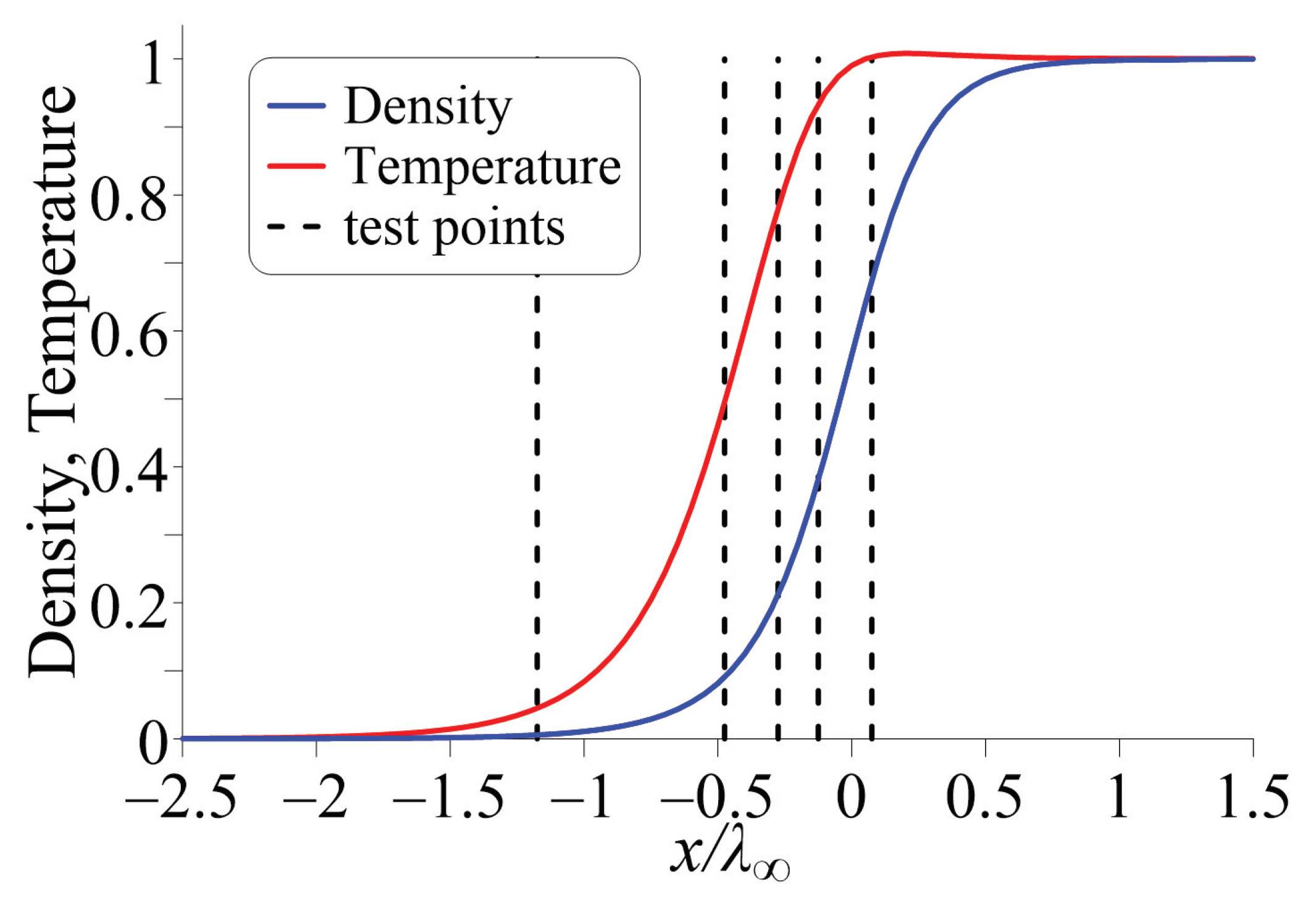
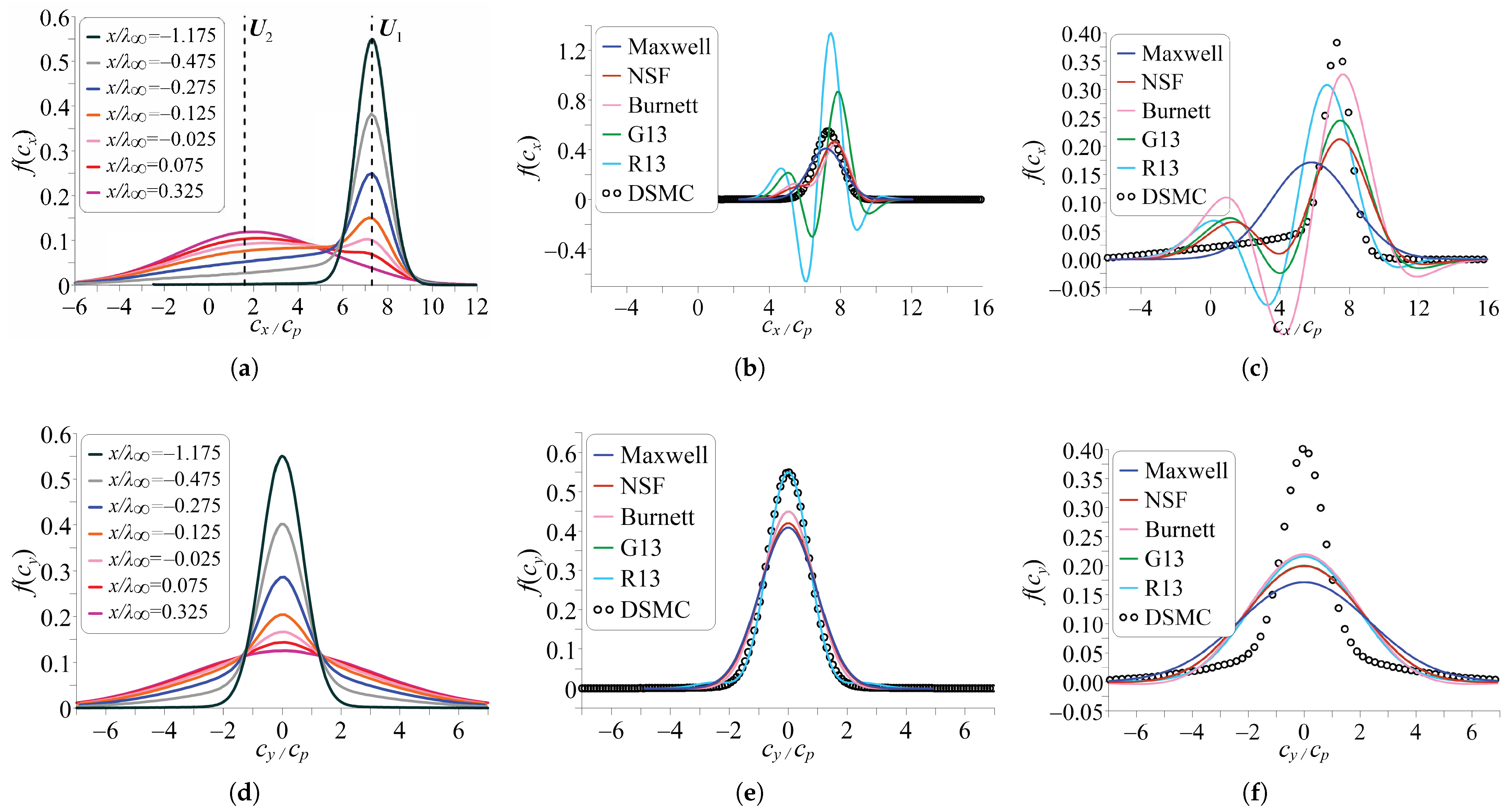
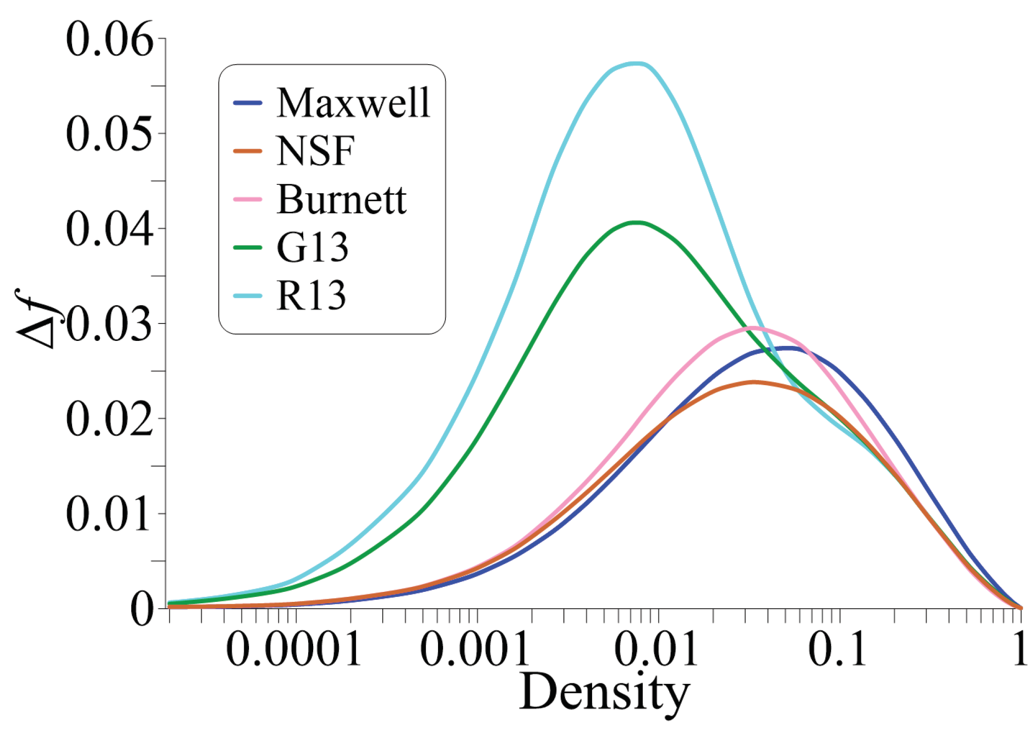
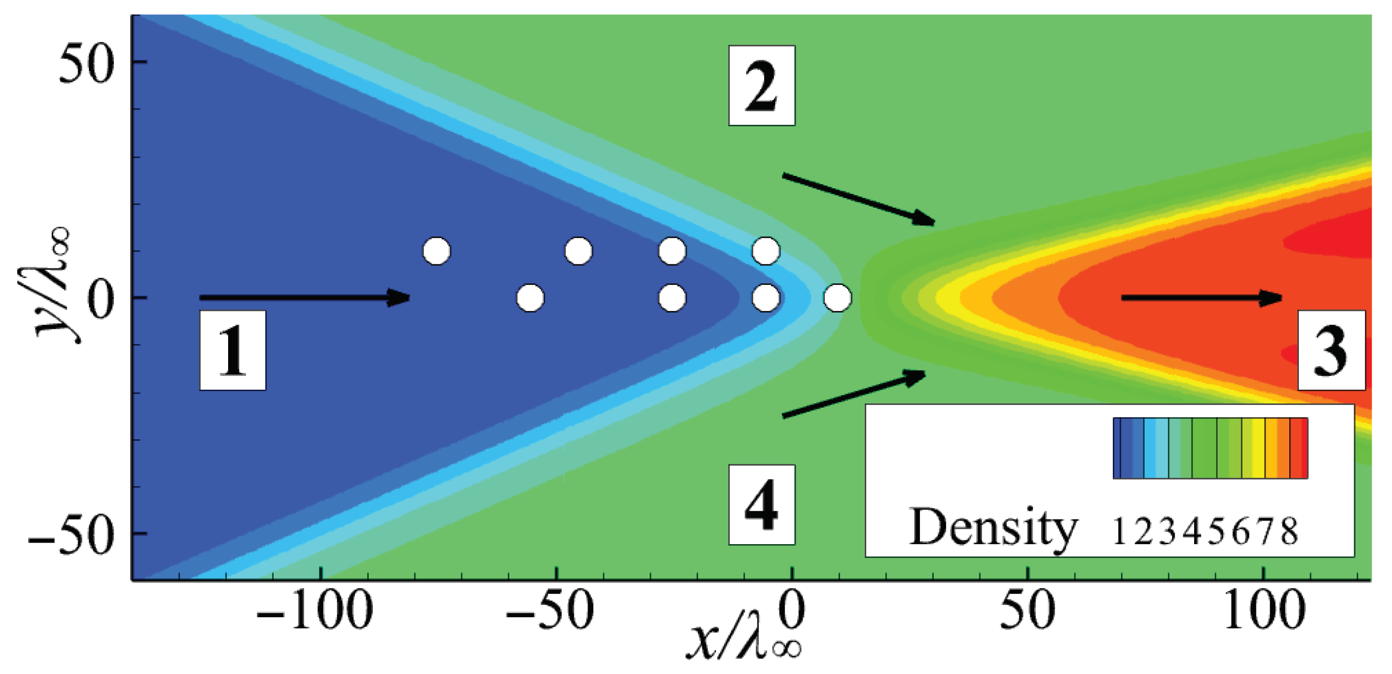
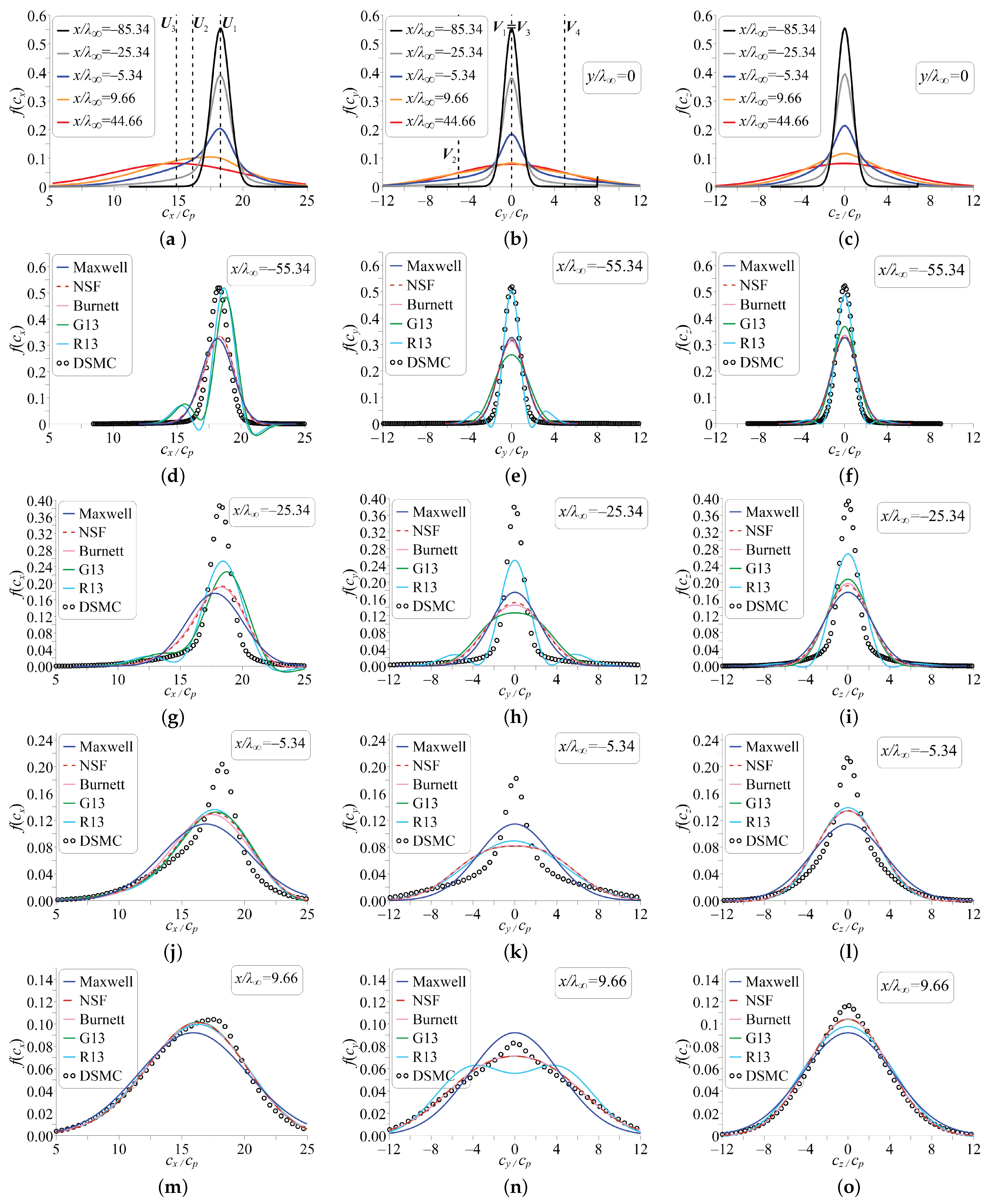
3.1. Shock Wave Structure

The one-dimensional planar shock wave structure in a monatomic gas is a classical problem of rarefied gas dynamics. Many publications have been devoted to analytical (see, e.g., Refs. [27,28,29]), numerical (see, e.g., Refs. [7,21,30,31,32,33]), and experimental (see, e.g., Refs. [34,35,36]) studies of this problem. The reference frame of the shock front is normally considered. Then, the boundary conditions are as follows: ${\rho }_1$, $u_1$, and ${\theta }_1$ are the values of density, velocity, and temperature at the upstream inflow boundary, while ${\rho }_2$, $u_2$, and ${\theta }_2$, which can be determined by the Rankine–Hugoniot relations [37], are the values at the downstream outflow boundary.

Figure 1 demonstrates the DSMC density and temperature profiles for the Mach number $Ma=8.0$. The spatial coordinate is normalized by the free-stream mean free path, which, for the Maxwell molecules, is given by [4]

$${\lambda }_{\infty }=\sqrt{{\displaystyle \frac{2}{\pi }}}{\displaystyle \frac{{\mu }_1}{{\rho }_1\sqrt{{\theta }_1}}}.$$

(10)

The density and temperature are normalized here as follows:

$$\widehat{\rho }={\displaystyle \frac{\rho -{\rho }_1}{{\rho }_2-{\rho }_1}},\widehat{\theta }={\displaystyle \frac{\theta -{\theta }_1}{{\theta }_2-{\theta }_1}}.$$

(11)

The origin is placed to the point with a normalized density value of 0.5. The Knudsen number cannot be uniquely determined for this problem due to the lack of an explicit characteristic length scale. It is possible to determine the local Knudsen number through the gradients of macroparameters or from the deviation of nonequilibrium macroparameters from the NSF approximation [21,38]. The shock wave structure at $Ma=8.0$ is quite an extreme case for macroscopic flow models due to a significant degree of flow nonequilibrium [39,40]. In this case, the local Knudsen number varies in a wide range from 0 to 0.5 in various parts of the flow [21].

The local molecular distribution function was obtained via the DSMC computations at various locations inside the shock wave front. The distribution functions for the macroscopic models under consideration were reconstructed at the same locations using the DSMC macroparameter data. The velocity distribution functions obtained via the DSMC computations are shown in Figure 2. The distribution function of molecular velocity $c_x$ in the x direction and the dimensionless molecular velocity ${\widehat{c}}_x$ are defined as follows (the definitions for the y and z directions are similar):

$$f\left(c_i\right)=\underset{-\infty }{\overset{+\infty }{\int }}\underset{-\infty }{\overset{+\infty }{\int }}f(c_i,c_j,c_k)d{c}_{j}d{c}_k,{\widehat{c}}_i={\displaystyle \frac{c_i}{\sqrt{2{\theta }_1}}}.$$

(12)

The DSMC distribution functions inside the shock front have a typical bimodal shape based on the upstream and downstream Maxwellians centered in the upstream $U_1$ and downstream $U_2$ flow velocities, respectively.

The distribution functions for various macroscopic models were compared with each other and with the DSMC results in Figure 2 and Figure 3. The most difficult region of the shock wave structure to describe by macroscopic methods is the supersonic part (leading front) [14,39]. As can be seen from Figure 2, at the first point considered on the shock wave ($x/{\lambda }_{\infty }=-1.175$, $\widehat{\rho }=0.006$), the local function already begins to differ noticeably from the Maxwell distribution. There arises a distribution tail, which is formed by slow molecules. In other words, the mode of the distribution, which is responsible for the equilibrium values to the right of the shock wave, begins to grow. The distribution function of the x-velocity for the G13 and R13 models demonstrates extreme oscillations for the longitudinal (parallel to the flow) component of the molecular velocity and turns out to be strongly negative for some velocities. It is well known that even common macroscopic models, such as the NSF equations, can yield unphysical negative values of the phase density [1,7,12,41]. Here, one faces the restriction on the distribution of high-velocity molecules discussed in Ref. [42]. There is no convergence in the hierarchy considered in this case. For the case of the shock wave structure with the free-stream Mach number $Ma=8.0$ under consideration, the convergence of the continuum approximations will be observed at the local Mach number $Ma<1.4$. The results for all other models for the longitudinal molecular velocity are much closer to the DSMC predictions.

Moving farther downstream (with a decrease in the local Mach number) leads to a more pronounced low-velocity tail of the DSMC distribution at high speeds. For the second point ($x/{\lambda }_{\infty }=-0.475$, $\widehat{\rho }=0.091$), the G13 and R13 models predict parallel velocity distributions, which are much closer to the DSMC results than those at the first point, the former does not even exhibit any negative values. On the other hand, the NSF and Burnett approximations demonstrate much stronger oscillations than those at the first point; in the latter case, the distribution even reaches the highest negative values among all the models. In general, all the macroscopic models in the study have qualitatively similar distributions with two local maxima and two local minima. The distributions of the perpendicular velocity for all the models look much more typical for both points and resemble a Gaussian bell curve.

The distributions at the third point ($x/{\lambda }_{\infty }=-0.275$, $\widehat{\rho }=0.214$) look qualitatively similar, but less extreme; it is only the Burnett model that has some negative-value intervals in the distribution of parallel molecular velocity. At the fourth point ($x/{\lambda }_{\infty }=-0.125$, $\widehat{\rho }=0.384$), the low-velocity tail starts forming into the downstream Maxwellian, and the DSMC distribution has a clear bimodal shape. All macroscopic-model distributions become much less oscillating and have only one maximum and no negative parts. At the last point considered ($x/{\lambda }_{\infty }=0.075$, $\widehat{\rho }=0.676$), which lies downstream of the shock center, the DSMC distributions are near-equilibrium with only a small “bump” on both parallel and perpendicular velocity distributions, indicative of the high-velocity Maxwellian. All macroscopic-model distributions are really close to each other at this point.

One can conclude that all macroscopic models considered predict the velocity distribution function in the low-density upper-front part of the shock rather poorly. To evaluate this discrepancy, the integral error of all approximations of the distribution function was calculated using a typical $L_2$ metrics expression:

$$\Delta f={\left[\sum _{i=1}^3{\int }_{-\infty }^{+\infty }{\left(f\left(c_i\right)-f_{\mathrm{DSMC}}\left(c_i\right)\right)}^{2}d{c}_i\right]}^{{\displaystyle \frac{1}{2}}}.$$

(13)

Note that various classical distribution-based measures (e.g., Kullback–Leibler divergence, entropy-based measures, or the Wasserstein distance) are used for positive functions and not directly applicable here, as all approximations considered except for the Maxwell distribution have negative value regions [43,44]. In contrast, the $L_2$ norm is suitable for the present task, because it can be used for functions having negative values and strongly penalizes significant local departures from the benchmark DSMC distribution observed in Equation (12).

The integral error is presented as a function of the local normalized density in Figure 4. Note that this definition of the error is not invariant with respect to rotations because the compared phase densities f and $f_{\mathrm{DSMC}}$ are integrals given by Equation (12), which depend on the frame of reference. Moreover, the Burnett equations are not invariant to rotations themselves [1,7]. That is why the presented error data should be considered only for the qualitative analysis of the macroscopic models. The integral error for some particular density values is presented in numerical form in

Table 1. Errors of the phase density approximations by various macroscopic models for the structure of a planar shock wave.

$\widehat{\mathit{\rho }}$	Maxwell	NSF	Burnett	G13	R13
0.0001	0.00043	0.00051	0.00051	0.00239	0.00302
0.001	0.00370	0.00429	0.00440	0.01803	0.02419
0.01	0.01898	0.01919	0.02252	0.03986	0.05394
0.1	0.02488	0.02018	0.02303	0.01999	0.01911
1	0.00000	0.00000	0.00000	0.00000	0.00000

.

The results confirm that the highest error at lower density is observed for models based on Grad’s method: G13 and R13. The error for these models grows until reaching the maximum at normalized density value of about 0.01. The errors for the other models while being several times lower than for the former two grows until the normalized density values of about 0.03–0.06. For intermediate densities close to 0.1, the error of models based on Grad’s method becomes smaller than that of the other models. It is interesting to note that the equilibrium Maxwell distribution clearly has a higher error than all other considered nonequilibrium models only for densities higher than 0.1.

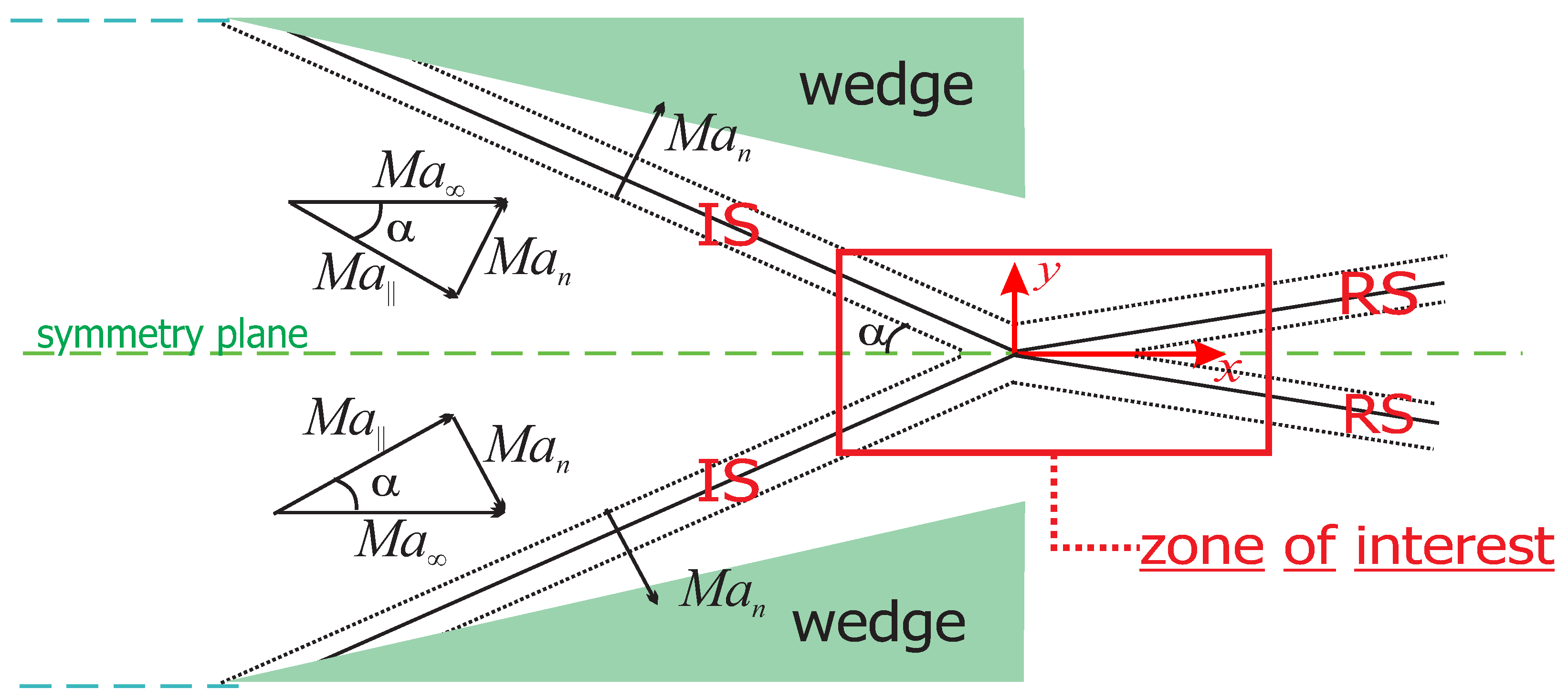
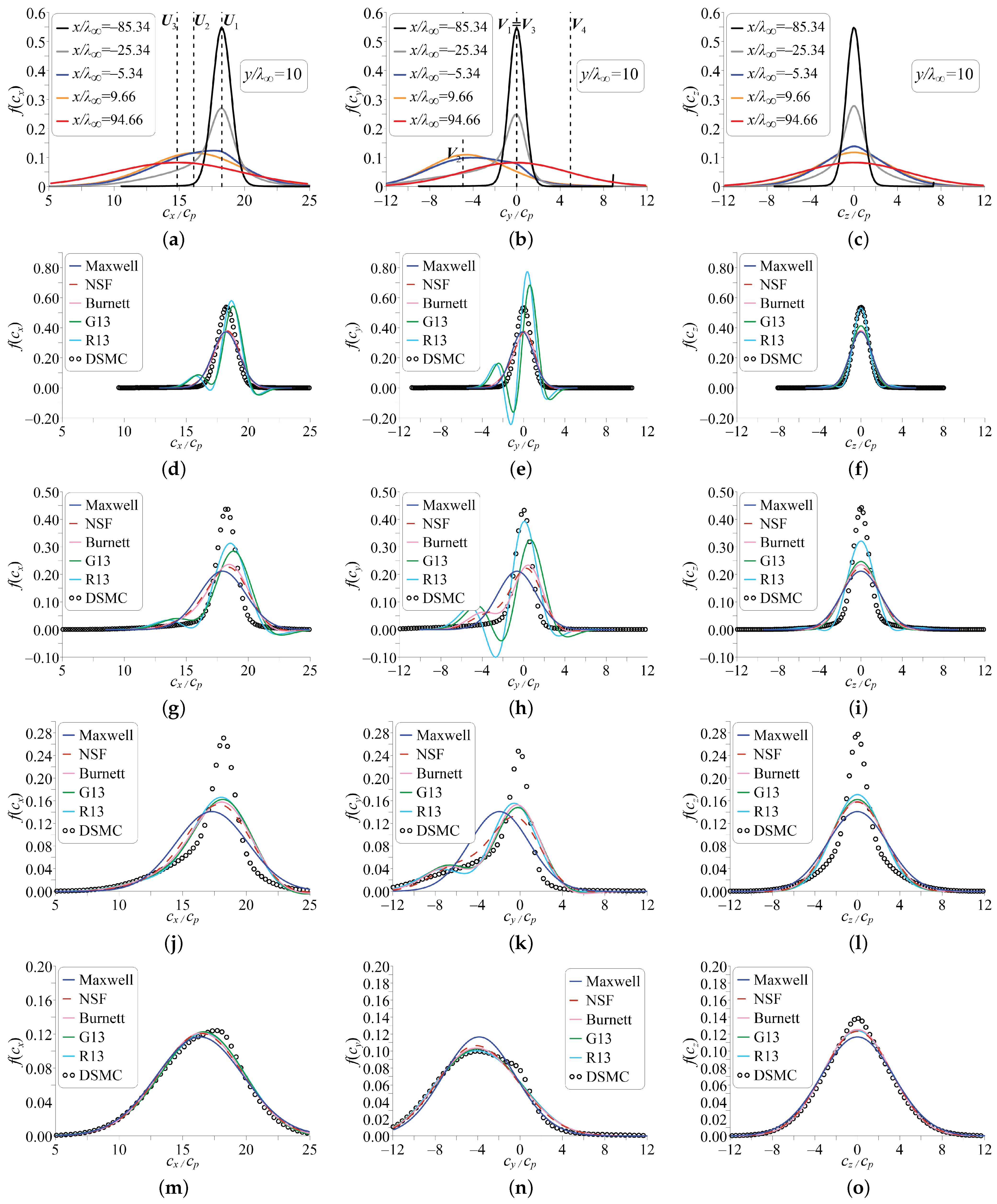
3.2. Regular Reflection of Shock Waves

If a pair of wedges is placed symmetrically in a uniform two-dimensional supersonic flow with a Mach number $Ma$, two oblique shock waves generated by the wedges interact on the symmetry plane. The simplest possible pattern of interaction is called the regular reflection. A schematic of such flow for a case when viscosity is taken into account and shock waves have finite thickness is presented in Figure 5. Interacting incident shock waves are denoted as IS here, while reflected shock waves are labeled RS. In the present study, a test case of the regular reflection flow from Ref. [20] is considered with only one difference: the viscosity–temperature index $\omega$ is assumed to be equal to unity. While the free-stream Mach number is equal to $Ma=20.0$, the Mach number along the normal to the oblique incident shock wave, as in the one-dimensional shock wave structure, is chosen to be equal to $M{a}_n=8.0$.

Only the flow in the vicinity of the reflection point is examined in the present study (see “zone of interest” in Figure 5). This flow region is illustrated with the DSMC flow field of density normalized with its free-stream value, which is presented in Figure 6. Such a flow structure, similarly to the structure of the planar shock, depends only on one length scale—the mean free path. Another similarity to the planar shock is the presence of a trivial analytical solution in the inviscid case (four uniform flow regions divided by discontinuities). When viscous and nonequilibrium effects are introduced, the flow becomes much more complicated and exhibits nontrivial features, such as a wake behind the reflection point (see Refs. [20,45,46] for more details). The velocity distribution function for this problem, on one hand, exhibits the modal nature inside the nonequilibrium regions as for the planar shock; on the other hand, however, it lacks symmetry inherent to the latter and, hence, has a more complicated shape (see Refs. [47,48]). The procedure for obtaining macroscopic approximations of the molecular distribution function using the DSMC results for the regular reflection problem is similar to that in the one-dimensional planar shock case.

The distribution functions along the symmetry plane ($y=0$) obtained in the DSMC computations are presented in the upper row of Figure 7. The distributions look qualitatively similar to that for the normal shock. The x-components $U_i$ and y-components $V_i$ of the gas flow velocities in the four flow zones presented in Figure 6 are shown by the vertical dashed lines on the plots. The slow-velocity tail of the distribution function of the x-velocity is centered about the gas velocity in the downstream region 4, which lies behind two oblique shocks (see Figure 6). The distributions of the y- and z-components of the molecular velocity look similar, though do not exactly coincide (see, e.g., the orange curves for $x/{\lambda }_{\infty }=39.66$, which demonstrate a wider distribution for the x-velocity). In general, the phase density exhibits a bimodal shape defined by the Maxwell distributions of zones 1 and 4.

The distribution functions predicted by various models were compared along the symmetry plane at points shown by white circles in Figure 6 (the lower row of circles). The comparison is illustrated in Figure 7. The first point ($x/{\lambda }_{\infty }=-75.34$) demonstrates high fluctuations of the G13 and R13 distributions with clear negative values for the x- and y-velocities, while the NSF and Burnett distributions are much closer to the equilibrium curve. An almost similar behavior of the distributions is observed at the second point ($x/{\lambda }_{\infty }=-45.34$). With a further increase in density, the distribution functions start to “normalize” and look much more like Gaussian bell curves at the third point ($x/{\lambda }_{\infty }=-25.34$). At the last point under consideration ($x/{\lambda }_{\infty }=-5.34$) with the DSMC distribution approaching the equilibrium shape, all the macroscopic models predict the phase density rather well, except for the R13 equations, which predict the y-velocity distribution with a minimum in the center. Farther downstream, all macroscopic models provide the phase density quite close to the DSMC results.

As it was demonstrated in Ref. [20], the gradients in the y direction in this particular test case are much greater than those in the x direction. That is why it is expected that the distribution functions are changed significantly with a variation in the y coordinate. In the upper row of Figure 8, the DSMC distribution functions along the line $y/{\lambda }_{\infty }=10$ are shown. The distributions of the x and z velocities are not affected significantly in comparison with the situation at the symmetry plane. It is interesting to note that the y-velocity distribution is changed drastically: the distributions in locations between zones 1 and 3 become clearly asymmetrical and centered around the gas velocity in zone 2 ($V_2$). It is possible to conclude that the phase density even only slightly above the symmetry plane is clearly three-modal with the modes defined by the flow parameters in zones 1, 3, and 2 (1, 3, and 4 for locations below the symmetry plane).

The phase densities for the macroscopic models are compared along the line $y/{\lambda }_{\infty }=10$ at the points denoted by the white circles (upper row) in Figure 6. The results are presented in Figure 8. The main difference from the similar results for the symmetry plane is much higher oscillations of the distribution functions of the y-velocity (central column). In particular, the G13 and R13 distributions reach significant negative values (less than −0.1). These oscillations escape when moving downstream, and all the macroscopic models are increasingly better at predicting data that are consistent with the DSMC results with an increase in density, as was observed for the symmetry plane plots and the planar shock results.

4. Conclusions

The molecular velocity distribution functions predicted by various macroscopic models of the monatomic gas flow were compared to the benchmark DSMC solution for the planar shock wave and the stationary regular shock wave reflection problem. Strong shock waves with the Mach number of 8 were considered for both problems, which provided a significant degree of flow nonequilibrium, and a non-Maxwellian, multimodal shape of the DSMC velocity distribution function. It can be concluded that all the macroscopic models predict the velocity distribution function rather poorly in the upstream low-density region, where the flow is essentially nonequilibrium. Not only is the error of approximation high, but unphysical oscillations of the phase density with highly negative values are also observed. Surprisingly, it is the most sophisticated and accurate model (in terms of predicting macroparameter distributions) as the R13 system of equations is the poorest in predicting nonequilibrium distributions. All the oscillations and discrepancies between the models gradually vanish when moving downstream, towards higher-density and more-equilibrium local conditions. All the macroscopic models predict the downstream part of the flow in both problems rather well.

While the possibility of negative values in velocity distribution functions predicted by various macroscopic gas dynamic models is well documented (see, e.g., Refs. [1,7,49,50]), the accuracy of the phase density representation by these models in strongly nonequilibrium conditions is widely ignored in the literature. The model testing is mostly focused on the comparison of macroparameter flow fields which are much closer to practice [51]. Possible remedies to the problem of inaccurate and even nonphysical forms of the distribution functions have not been suggested yet to the best of the authors’ knowledge. One may argue that these macroscopic models were not constructed to be used in conditions far from equilibrium in the first place. Nonetheless, the results of the present study support the notion that even most accurate and well-validated macroscopic models should be applied to flows with strong shock waves with great caution.

References

1. Cercignani, C. The Boltzmann Equation and Its Applications; Springer: Berlin/Heidelberg, Germany, 1988. [Google Scholar]
2. Sitnikov, S.; Tcheremissine, F. A method for numerical simulation of shock waves in rarefied gas mixtures based on direct solution of the Boltzmann kinetic equation. J. Comput. Phys. 2025, 520, 113463. [Google Scholar] [CrossRef]
3. Wu, L.; Zhang, J.; Reese, J.M.; Zhang, Y. A fast spectral method for the Boltzmann equation for monatomic gas mixtures. J. Comput. Phys. 2015, 298, 602–621. [Google Scholar] [CrossRef]
4. Bird, G.A. Molecular Gas Dynamics and the Direct Simulation of Gas Flows; Clarendon Press: Oxford, UK, 1994. [Google Scholar]
5. Boyd, I.D.; Schwartzentruber, T.E. Nonequilibrium Gas Dynamics and Molecular Simulation; Cambridge University Press: Cambridge, UK, 2017. [Google Scholar]
6. Ivanov, M.S.; Gimelshein, S.F. Computational Hypersonic Raredied Flows. Annu. Rev. Fluid Mech. 1998, 30, 469–505. [Google Scholar] [CrossRef]
7. Struchtrup, H. Macroscopic Transport Equations for Rarefied Gas Flows; Springer: Berlin/Heidelberg, Germany, 2005. [Google Scholar]
8. Torrilhon, M. Modeling Nonequilibrium Gas Flow Based on Moment Equations. Annu. Rev. Fluid Mech. 2016, 48, 429–458. [Google Scholar] [CrossRef]
9. Kogan, M.N. Rarefied Gas Dynamics; Plenum: New York, NY, USA, 1969. [Google Scholar]
10. Chapman, S.; Cowling, T.G. The Mathematical Theory of Non-Uniform Gases: An Account of the Kinetic Theory of Viscosity, Thermal Conduction and Diffusion in Gases; Cambridge Mathematical Library: Cambridge, UK, 1991. [Google Scholar]
11. Li, Q.; Zeng, J.; Wu, L. Kinetic modelling of rarefied gas mixtures with disparate mass in strong non-equilibrium flows. J. Fluid Mech. 2024, 1001, A5. [Google Scholar] [CrossRef]
12. Grad, H. On the kinetic theory of rarefied gases. Commun. Pure Appl. Math. 1949, 2, 331–407. [Google Scholar] [CrossRef]
13. Pham-Van-Diep, G.C.; Erwin, D.A.; Muntz, E.P. Testing continuum descriptions of low-Mach-number shock structures. J. Fluid Mech. 1991, 232, 403–413. [Google Scholar] [CrossRef]
14. Erofeev, A.I.; Friedlander, O.G. Macroscopic Models for Nonequilibrium Flows of Monatomic Gas and Normal Solutions. In Proceedings of the 25th International Symposium on Rarefied Gas Dynamics, Saint-Petersburg, Russia, 18–21 July 2007; pp. 117–124. [Google Scholar]
15. Ivanov, I.E.; Timokhin, M.Y.; Kryukov, I.A.; Bondar, Y.A.; Kokhanchik, A.A.; Ivanov, M.S. Study of the Shock Wave Structure by Regularized Grad’s Set of Equations. AIP Conf. Proc. 2012, 1501, 215–222. [Google Scholar] [CrossRef]
16. Westerkamp, A.; Torrilhon, M. Finite element methods for the linear regularized 13-moment equations describing slow rarefied gas flows. J. Comput. Phys. 2019, 389, 1–21. [Google Scholar] [CrossRef]
17. Matsubara, H.; Kikugawa, G.; Ohara, T. All- and one-particle distribution functions at nonequilibrium steady state under thermal gradient. Phys. Rev. E 2019, 99, 052110. [Google Scholar] [CrossRef]
18. Han, Q.; Xia, H.; Chen, W.; Wu, G.; Li, J.; Wei, Z.; Zheng, F.; Ma, C. Non-equilibrium molecular motion and interface heat transfer in supersonic rarefied flows. Phys. Fluids 2025, 37, 037132. [Google Scholar] [CrossRef]
19. Zarei, A.; Karimipour, A.; Meghdadi Isfahani, A.H.; Tian, Z. Improve the performance of lattice Boltzmann method for a porous nanoscale transient flow by provide a new modified relaxation time equation. Phys. A Stat. Mech. Its Appl. 2019, 535, 122453. [Google Scholar] [CrossRef]
20. Bondar, Y.A.; Shoev, G.V.; Timokhin, M.Y. Regular reflection of shock waves in steady flows: Viscous and non-equilibrium effects. J. Fluid Mech. 2024, 984, A10. [Google Scholar] [CrossRef]
21. Timokhin, M.Y.; Struchtrup, H.; Kokhanchik, A.A.; Bondar, Y.A. The analysis of different variants of R13 equations applied to the shock-wave structure. AIP Conf. Proc. 2016, 1786, 140006. [Google Scholar] [CrossRef]
22. Zheng, Y.; Struchtrup, H. Burnett equations for the ellipsoidal statistical BGK model. Contin. Mech. Thermodyn. 2004, 16, 97–108. [Google Scholar] [CrossRef]
23. Gu, X.J.; Emerson, D.R. A high-order moment approach for capturing non-equilibrium phenomena in the transition regime. J. Fluid Mech. 2009, 636, 177–216. [Google Scholar] [CrossRef]
24. Shevyrin, A.; Bondar, Y.; Ivanov, M. Analysis of Repeated Collisions in the DSMC Method. AIP Conf. Proc. 2005, 762, 565–570. [Google Scholar] [CrossRef]
25. Ivanov, M.; Markelov, G.; Gimelshein, S. Statistical simulation of reactive rarefied flows—Numerical approach and applications. In Proceedings of the 7th AIAA/ASME Joint Thermophysics and Heat Transfer Conference (AIAA 1998–2669), Albuquerque, NM, USA, 15–18 June 1998; p. 2669. [Google Scholar] [CrossRef]
26. Ivanov, M.S.; Kashkovsky, A.V.; Vashchenkov, P.V.; Bondar, Y.A. Parallel Object-Oriented Software System for DSMC Modeling of High-Altitude Aerothermodynamic Problems. AIP Conf. Proc. 2011, 1333, 211–218. [Google Scholar] [CrossRef]
27. Becker, R. Stoßwelle und Detonation. Z. Physik. 1922, 8, 321–362. [Google Scholar] [CrossRef]
28. Mott-Smith, H.M. The Solution of the Boltzmann Equation for a Shock Wave. Phys. Rev. 1951, 82, 885–892. [Google Scholar] [CrossRef]
29. Yen, S.M. Temperature Overshoot in Shock Waves. Phys. Fluids 1966, 9, 1417–1418. [Google Scholar] [CrossRef]
30. Xu, K.; Huang, J.C. A unified gas-kinetic scheme for continuum and rarefied flows. J. Comput. Phys. 2010, 229, 7747–7764. [Google Scholar] [CrossRef]
31. Ohwada, T. Structure of normal shock waves: Direct numerical analysis of the Boltzmann equation for hard-sphere molecules. Phys. Fluids A 1993, 5, 217–234. [Google Scholar] [CrossRef]
32. Zhang, Y.D.; Xu, A.G.; Zhang, G.C.; Chen, Z.H.; Wang, P. Discrete ellipsoidal statistical BGK model and Burnett equations. Front. Phys. 2018, 13, 135101. [Google Scholar] [CrossRef]
33. Zhu, Q.; Wu, Y.; Zhou, W.; Yang, Q.; Xu, X. A comprehensive study on the roles of viscosity and heat conduction in shock waves. J. Fluid Mech. 2024, 984, A74. [Google Scholar] [CrossRef]
34. Hansen, K.; Hornig, D.F. Thickness of Shock Fronts in Argon. J. Chem. Phys. 1960, 33, 913–916. [Google Scholar] [CrossRef]
35. Alsmeyer, H. Density Profiles in Argon and Nitrogen Shock Waves Measured by the Absorption of an Electron Beam. J. Fluid Mech. 1976, 74, 497–513. [Google Scholar] [CrossRef]
36. Pham-Van-Diep, G.; Erwin, D.; Muntz, E.P. Nonequilibrium Molecular Motion in a Hypersonic Shock Wave. Science 1989, 245, 624–626. [Google Scholar] [CrossRef]
37. Rankine, W.J.M. On the thermodynamic theory of waves of finite longitudinal disturbance. Philos. Trans. R. Soc. Lond. 1870, 160, 277–288. [Google Scholar] [CrossRef]
38. Lockerby, D.A.; Reese, J.M.; Struchtrup, H. Switching criteria for hybrid rarefied gas flow solvers. Proc. R. Soc. Math. Phys. Eng. Sci. 2009, 465, 1581–1598. [Google Scholar] [CrossRef]
39. Su, X.; Lin, C. Nonequilibrium effects of reactive flow based on gas kinetic theory. Commun. Theor. Phys. 2022, 74, 035604. [Google Scholar] [CrossRef]
40. Lin, C.; Su, X.; Zhang, Y. Hydrodynamic and Thermodynamic Nonequilibrium Effects around Shock Waves: Based on a Discrete Boltzmann Method. Entropy 2020, 22, 1397. [Google Scholar] [CrossRef] [PubMed]
41. Timokhin, M.; Rukhmakov, D. Local non-equilibrium phase density reconstruction with Grad and Chapman-Enskog methods. J. Phys. Conf. Ser. 2021, 1959, 012049. [Google Scholar] [CrossRef]
42. Cai, Z.; Torrilhon, M. On the Holway-Weiss debate: Convergence of the Grad-moment-expansion in kinetic gas theory. Phys. Fluids 2019, 31, 126105. [Google Scholar] [CrossRef]
43. Cover, T.M.; Thomas, J.A. Elements of Information Theory, 2nd ed.; Wiley-Interscience: Hoboken, NJ, USA, 2006. [Google Scholar]
44. Villani, C. Optimal Transport: Old and New; Grundlehren der mathematischen Wissenschaften; Springer: Berlin/Heidelberg, Germany, 2008; Volume 338. [Google Scholar]
45. Khotyanovsky, D.; Bondar, Y.; Kudryavtsev, A.; Shoev, G.; Ivanov, M. Viscous effects in steady reflection of strong shock waves. AIAA J. 2009, 47, 1263–1269. [Google Scholar] [CrossRef]
46. Gan, Y.; Zhuang, Z.; Yang, B.; Xu, A.; Zhang, D.; Chen, F.; Song, J.; Wu, Y. Supersonic flow kinetics: Mesoscale structures, thermodynamic nonequilibrium effects and entropy production mechanisms. arXiv 2025, arXiv:2502.10832. [Google Scholar]
47. Bondar, Y.; Shoev, G.; Kokhanchik, A.; Timokhin, M. Nonequilibrium velocity distribution in steady regular shock-wave reflection. AIP Conf. Proc. 2019, 2132, 120005. [Google Scholar] [CrossRef]
48. Timokhin, M.Y.; Kudryavtsev, A.N.; Bondar, Y.A. The Mott-Smith solution to the regular shock reflection problem. J. Fluid Mech. 2022, 950, A14. [Google Scholar] [CrossRef]
49. Müller, I.; Ruggeri, T. Rational Extended Thermodynamics; Springer: New York, NY, USA, 1998. [Google Scholar] [CrossRef]
50. Bobylev, A.V. Instabilities in the Chapman-Enskog Expansion and Hyperbolic Burnett Equations. J. Stat. Phys. 2006, 124, 371. [Google Scholar] [CrossRef]
51. Shakhov, E. The Method of Investigation of Motion of a Rarefied Gas; Nauka: Moscow, Russia, 1974. (In Russian) [Google Scholar]
Figure 1. Density and temperature profiles for the structure of a planar shock wave, M a = 8.0 .
Mathematics 13 01328 g001
Figure 2. Distribution functions of molecular velocity in directions parallel (upper row) and perpendicular (lower row) to the flow for the planar shock wave problem. DSMC results for various locations (lefta,d). Comparison of various models for x / λ = 1.175 , ρ ^ = 0.006 (centerb,e) and x / λ = 0.475 , ρ ^ = 0.091 (rightc,f).
Mathematics 13 01328 g002
Figure 3. Distribution functions of molecular velocity in directions parallel (upper row) and perpendicular (lower row) to the flow for the planar shock wave problem. Comparisons of various models for x / λ = 0.275 , ρ ^ = 0.214 (lefta,d); x / λ = 0.125 , ρ ^ = 0.384 (centerb,e) and x / λ = 0.075 , ρ ^ = 0.676 (rightc,f).
Mathematics 13 01328 g003
Figure 4. Errors of the phase density approximations by various macroscopic models for the structure of a planar shock wave.
Mathematics 13 01328 g004
Figure 5. Schematic of a steady viscous flow with regular reflection of shock waves.
Mathematics 13 01328 g005
Figure 6. DSMC density flow field in the vicinity of the regular reflection point.
Mathematics 13 01328 g006
Figure 7. Distribution functions of various components of molecular velocity along the symmetry plane ( y / λ = 0.0 ) in the regular reflection problem. DSMC (ac), x / λ = 55.34 (df), x / λ = 25.34 (gi), x / λ = 5.34 (jl), and x / λ = 9.66 (mo).
Mathematics 13 01328 g007
Figure 8. Distribution functions of various components of molecular velocity along the y / λ = 10.0 line in the regular reflection problem. DSMC (ac), x / λ = 75.34 (df), x / λ = 45.34 (gi), x / λ = 25.34 (jl), and x / λ = 5.34 (mo).
Mathematics 13 01328 g008