ParDP: A Parallel Density Peaks-Based Clustering Algorithm

Abstract

This paper proposes ParDP, an algorithm and concrete tool for unsupervised clustering, which belongs to the class of density peaks-based clustering methods. Such methods rely on the observation that cluster representative points (centroids) are points of higher local density surrounded by points of lesser density. Candidate centroids, though, are to be far from each other. A key factor of ParDP is adopting a k-Nearest Neighbors (kNN) technique for estimating the density of points. Complete clustering depends on densities and distances among points. ParDP uses principal component analysis to cope with high-dimensional data points. The current implementation relies on Java parallel streams and the built-in lock-free fork/join mechanism, enabling the exploitation of the computing power of commodity multi/many-core machines. This paper demonstrates ParDP’s clustering capabilities by applying it to several benchmark and real-world datasets. ParDP’s operation can either be directed to observe the number of clusters in a dataset or to finalize clustering with an assigned number of clusters. Different internal and external measures can be used to assess the accuracy of a resultant clustering solution.

1. Introduction

Unsupervised clustering [1] is a common technique for mining information from the sample data points of a dataset. Application domains include image segmentation, machine learning, artificial intelligence, medicine, biology, etc. The goal is to partition the points of a dataset, $X={\left\{x_i\right\}}_{i=1}^N$, into groups (said clusters) in such a way that the points of the same cluster are similar, but dissimilar to the points assigned to other clusters. Each cluster is characterized by a representative point called its centroid ${\mu }_j$. The similarity function often coincides with the Euclidean function when the dataset points are vectors with $D$ numerical coordinates (dimensions): $x_i\in R^D$.

An often-used centroids-based clustering algorithm is K-Means [2,3], where the number $K$ of clusters/centroids is an input parameter. K-Means’s recurrent use owes to its simplicity and efficiency [4]. K-Means, though, is more suited to datasets with spherical clusters. In addition, it strongly depends on the initialization of centroids (seeding) [5,6]. A bad initialization quickly causes K-Means to become stuck in a local sub-optimal solution. K-Means acts as a local refiner of centroids and cannot search for centroids globally in the dataset. To control these limitations, careful seeding methods can be used [7,8,9] together with the concept of repeating it many times (Repeated K-Means), each time with a different initialization, toward the obtainment of an acceptable solution, as mirrored by some clustering accuracy measures. Random Swap [10,11] integrates K-Means in its behavior and bases its operation on a global search for centroids. At each iteration, a swap is accomplished, which replaces a randomly chosen centroid with a randomly selected dataset point. Provided a suited number of swap iterations are executed, Random Swap has been proven to be able, in many cases, to find a solution close to the optimal one.

A different yet popular clustering algorithm, designed for non-spherical clusters, is based on the concept of density peaks (DP) [12]. DP relies on the fact that, naturally, centroids are points of higher local density, whose neighborhood is made up of points with lesser density. In addition, a candidate centroid is a point of higher density relatively far from points with a higher density. Two data point quantities regulate the application of DP: density (rho) and minimal distance to the nearest point with a higher density (delta). A fundamental problem is the estimation of the point density. In the original proposal [12], the concept of a cutoff distance $d_c$ (distance threshold) is introduced. Such distance is the radius of a hyperball in the D-dimensional space. The density is established by (logically) counting points that fall in the ball. The authors in [12] adopted the “thumb rule” of choosing a value for $d_c$, which can ensure that from 1% to 2% of the dataset, the number of points falls in the hyperball. DP clustering is finalized by considering both the rho and delta values of points. Centroids are chosen as points with high values of both rho and delta. The remaining points are assigned to clusters/centroids according to the delta attribute. However, it has been pointed out that the DP basic approach cannot recognize clusters with an arbitrary geometry.

In the last few years, several proposals appeared in the literature to improve specifically the estimation of density and thus handling clusters of an arbitrary shape. A notable class of works is based on the k-Nearest Neighbors (kNN) technique, with $k$ as an input parameter. In [13], from the $k$-th Nearest Neighbor distance of a data point, p, indicated as ${NN}_k\left(p\right)$, the kNN neighborhood of a data point, p (${kNN}_k\left(p\right)$), is first defined: ${kNN}_k\left(p\right)=\left\{q\in X|d\left(p,q\right)\le {NN}_k\left(p\right)\right\}$, where $d(p,q)$ is the distance between p and q. Then, the local density of p is inferred through a Gaussian exponential kernel. The proposal in [13] adds to the clustering method the principal component analysis (PCA) to deal with the “curse of dimensionality”, that is, the problem of a high number of point coordinates (dimensions) that can cause the Euclidean distance to lose its meaning. A (hopefully) reduced number of coordinates is preliminarily detected to guarantee data variations and the consistency of the Euclidean distance.

The kNN approach was further specialized with the concepts of reverse and natural Nearest Neighbors [14,15]. From the k-th nearest point of a point, p, ${NN}_k\left(p\right)$, the Reverse Nearest Neighbors (RNN) of p, $RNN\left(p\right)$, is defined as the set of points, q, which have p within the distance ${NN}_k\left(q\right)$, that is: $RNN\left(p\right)=\left\{q\in X\right| d(p,q)\le {NN}_k\left(q\right)\}$. Two nearest neighbor points, p and q, are said natural neighbors when, as in the friendship relationship of human societies, each one belongs to the RNN of the partner: $p\in RNN\left(q\right)\wedge q\in RNN\left(p\right)$. A further concept concerns the definition of the Mutual Nearest Neighbors (NMM) set of a point, p, defined as: $MNN\left(p\right)={kNN}_k\left(p\right)\cup RNN\left(p\right)$. A benefit of the RNN-based approaches in [14,15] is the possibility of inferring a suitable value of $k$ in the algorithm, by automatically checking different radius values, starting from 2, until a stable search state is reached, where the friendship relation among points stabilizes.

A common problem of density estimation by kNN-based approaches is the high computational cost, $O\left(N^2\right)$, due to the need to compute all the pairwise distances of points. Such a cost can limit the applicability of kNN to large datasets. Fränti et al. [16,17] developed a fast-density peak algorithm (FastDP) based on the approximate construction of the $kNN$ graph through an efficient divisive technique. The divisive technique randomly selects two points, $a$ and $b$, in the dataset, and then the points of the dataset are partitioned into two groups according to the nearer distance from $a$ or $b$. The two sub-sets are recursively split until their size appears under a given threshold, in which case a corresponding kNN subgraph is directly built (brute force). The divisive technique is repeated many times in the algorithm’s first part until the edge changes in the last iteration becomes smaller than a given tolerance. In the second part, the divisive technique is continued by combining sub-graphs by neighborhood propagation (NN-Descent method [16,18]), that is by evaluating neighbors of neighbors. Instead of creating the graph from scratch, the previous graph is updated by reviewing the k-Nearest Neighbors of each point by considering the information that emerged in the latest solution. The approximate kNN graph is finally used to estimate each point’s density and delta values. Density is evaluated as the inverse of the mean distance to the k-Nearest Neighbors. As demonstrated in [16], FastDP can handle different data types, provided a distance function is available.

This paper proposes ParDP, a density peaks-based algorithm and tool that depends on kNN to estimate density. ParDP does not build an approximate KNN graph as in [16]. Anyway, the $O\left(N^2\right)$ cost is smoothed by exploiting Java parallelism [4,9,11,19].

A preliminary version of ParDP, where a suitable global value, $d_c$, was initially tentatively tuned, was presented as a conference paper [20]. Concerning the conference paper, the following new contributions are added.

• Using the kNN approach for inferring points’ density and delta values. In particular, ParDP can exploit kNN for inferring a global value of $d_c$ from which a Gaussian kernel evaluates densities. Alternatively, densities can directly be estimated from the kNN distances.
• Supporting the principal component analysis (PCA) for (hopefully) reducing the high number of dimensions of some datasets while preserving the meaning of the Euclidean distance.
• Optimizing the use of Java parallel streams [19] in all the basic steps of ParDP, ranging from evaluating the density and delta values to final clustering to implementing various clustering measures.
• Applying ParDP to several benchmark and real-world datasets.
• Adapting the Java implementation of ParDP for an achievement, PCA included, of the Du et al. [13] density peaks algorithm (here referred to as ParDPC-KNN) as well as a density peaks algorithm based on the Mutual Nearest Neighbors (MNN) approach [19] (here referred to as ParDPC-MNN).
• Verifying ParDP correctness and performance by comparing it to ParDPC-KNN and ParDPC-MNN.

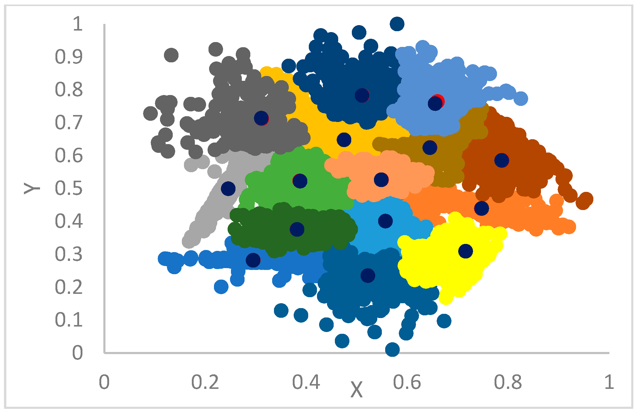
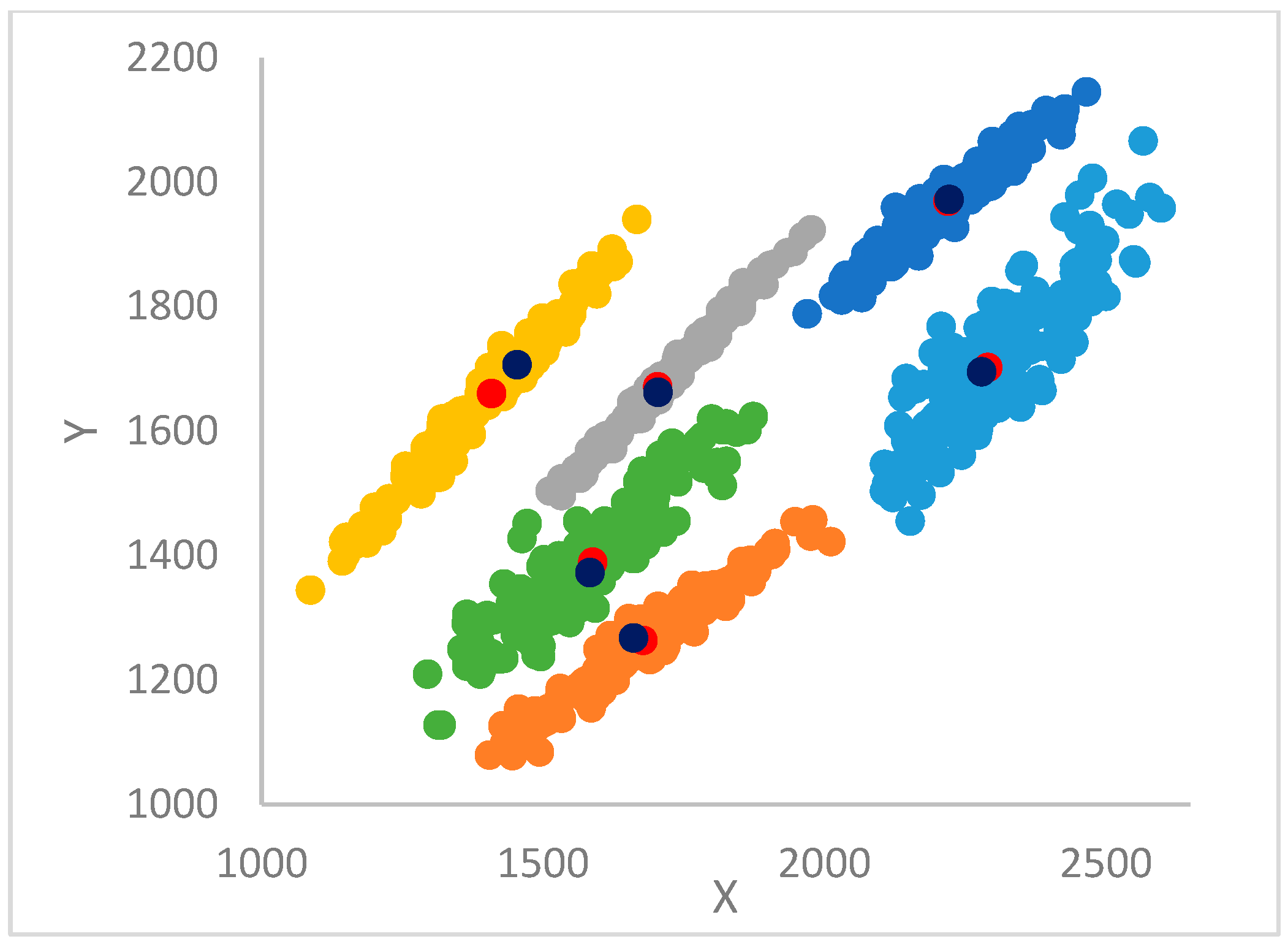
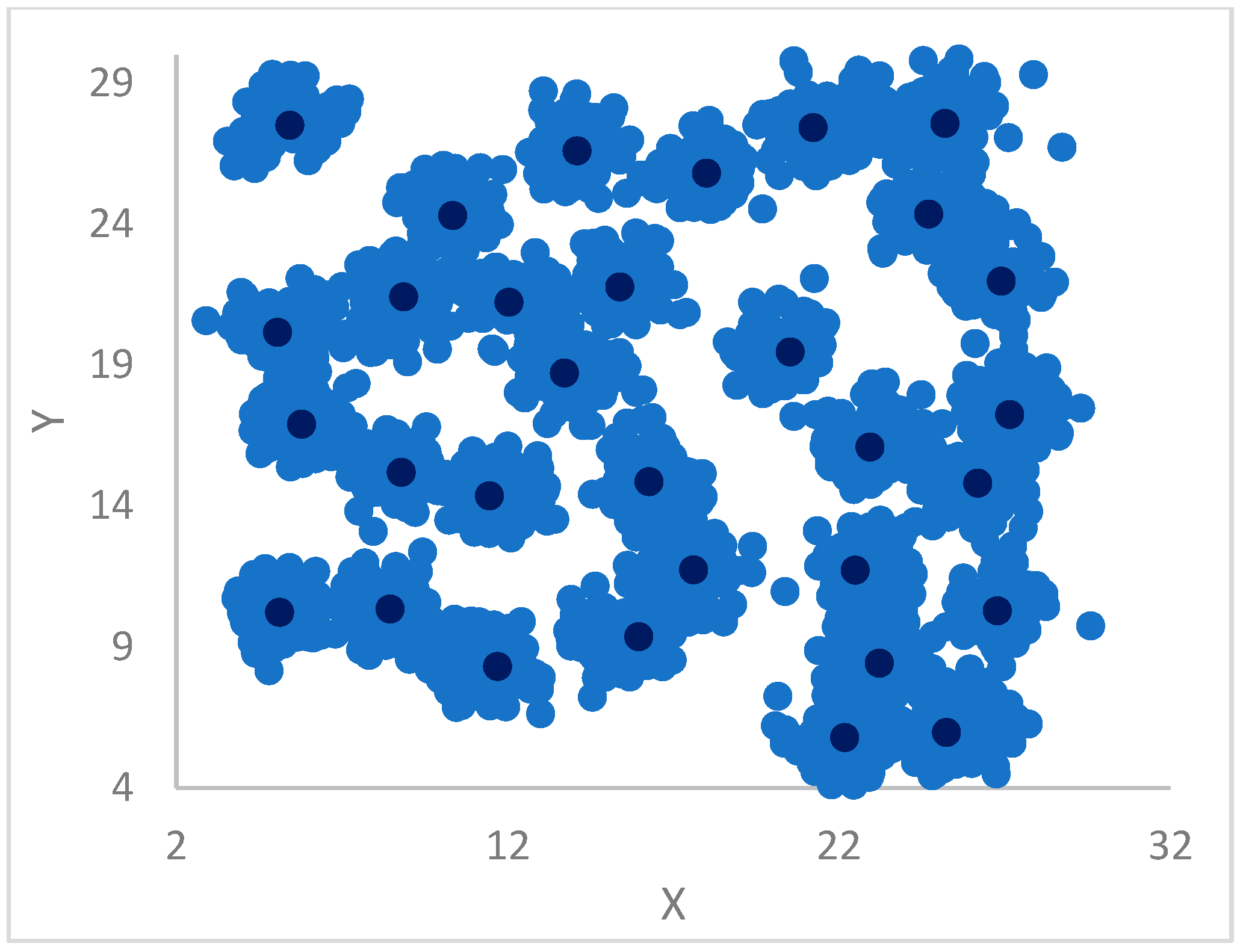
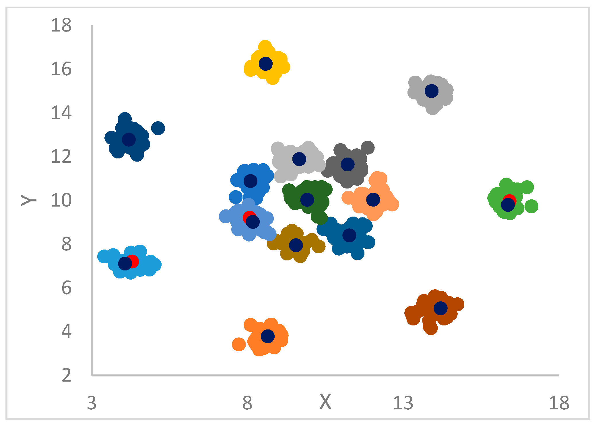
This paper is structured as follows. Section 2 reviews the fundamental concepts of the basic density peaks clustering algorithm (DP). Section 3 discusses the design and implementation aspects of the proposed ParDP algorithm. Section 4 provides a summary of the clustering accuracy indexes used in the practical experiments. Section 5 is devoted to the experimental work. ParDP is applied to 23 challenging synthetic and real-world datasets, split into three groups. The clustering results are compared with those achieved by competing tools. Finally, Section 6 draws some conclusions about the developed work and indicates directions for future work.

2. Density Peaks-Basic Algorithm

The density peaks basic algorithm (DP) [12] rests on the intuition that centroids are points of higher local density, surrounded by points of lesser density. As a consequence, a centroid is relatively distant from other points of a higher density. To formalize this intuition, two quantities are introduced for each point, $x_i$: its density ($\rho$) and its nearest distance ($\delta$) to a point with a higher density. Such a nearest point is called, in [16,17], the big brother of $x_i$. It is evident that for a point to be a candidate centroid, it should have a high value of both $\rho$ and $\delta$. 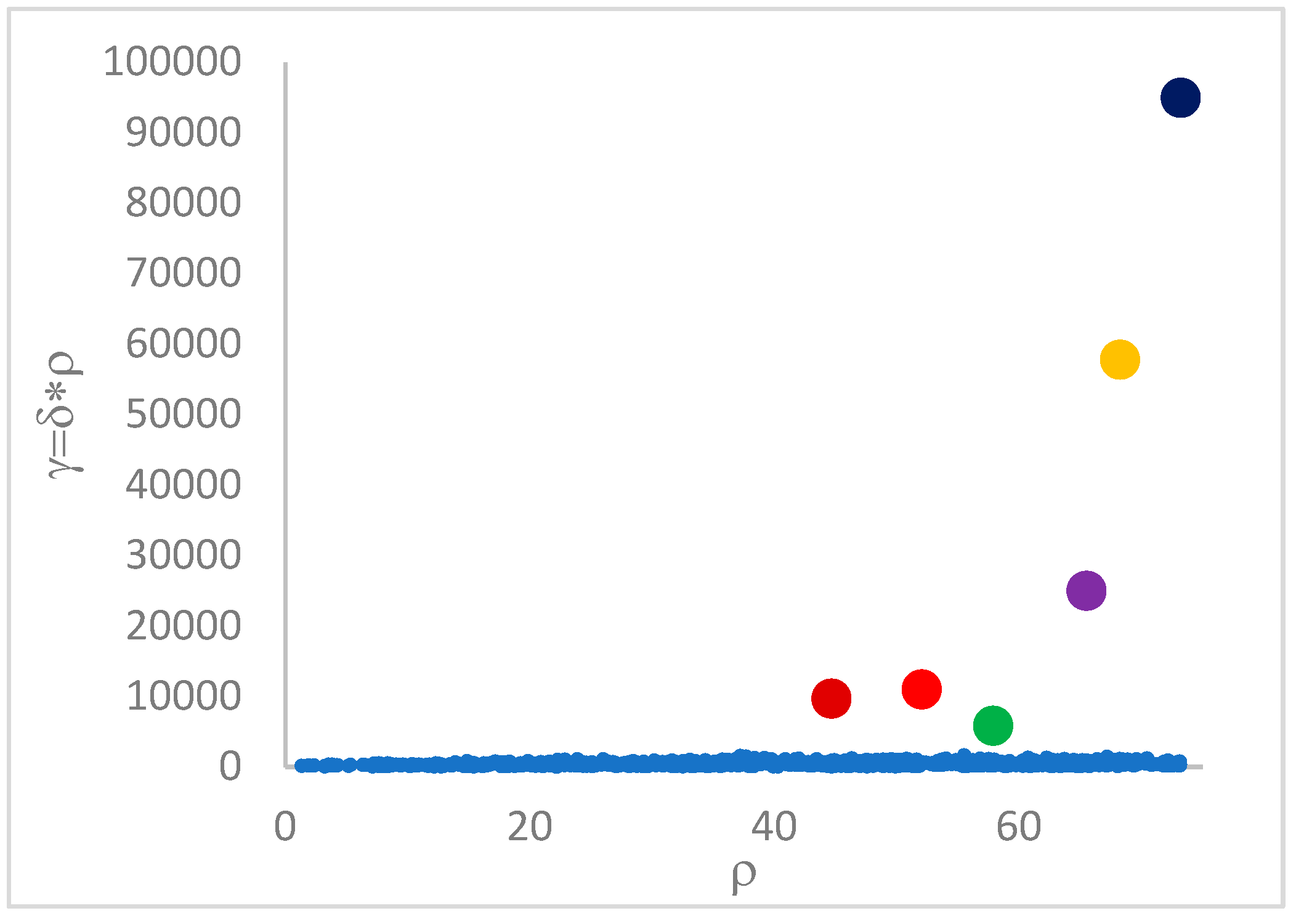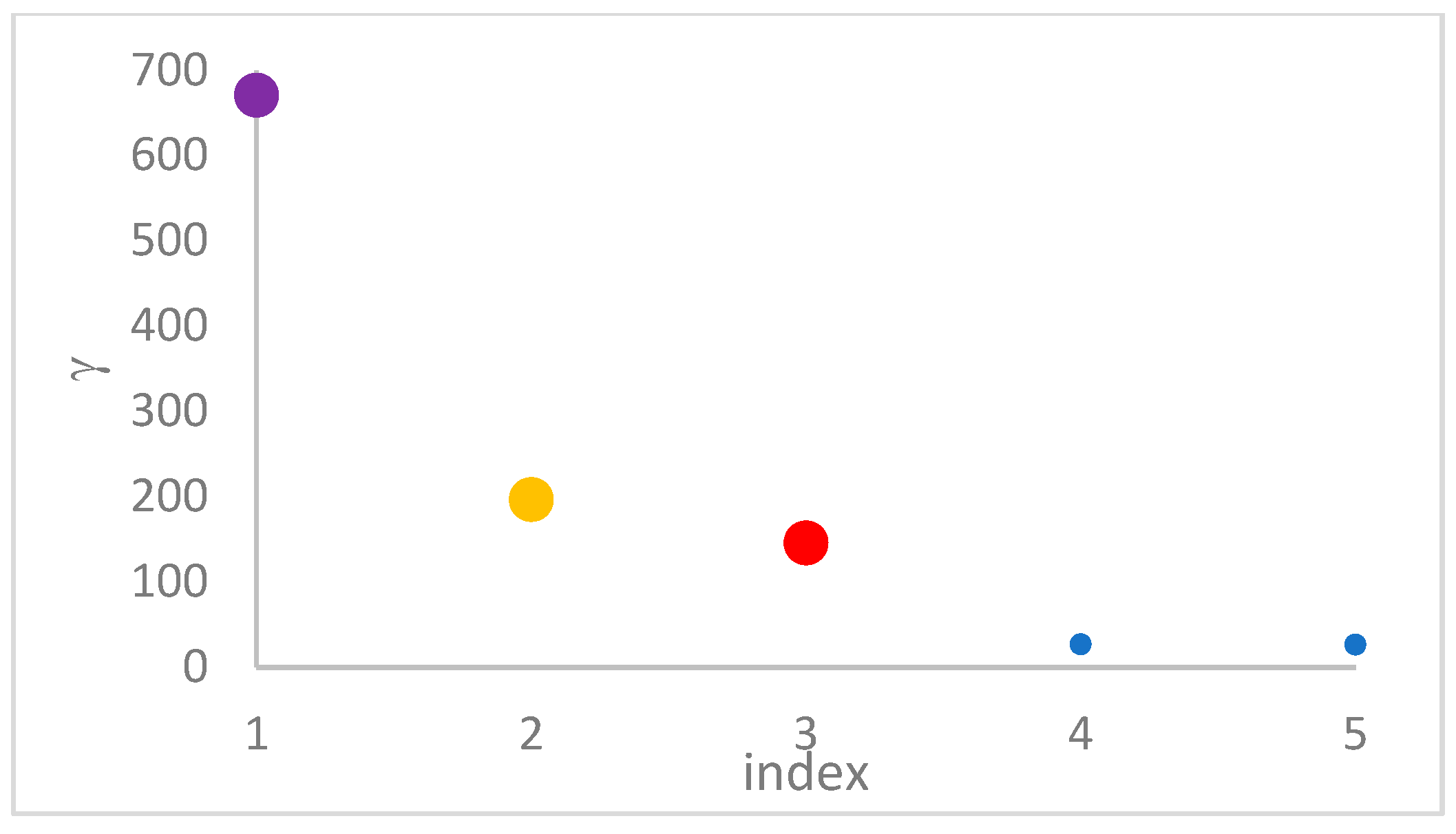Equivalently, a candidate centroid should have a high value of a third quantity, (gamma) $\gamma =\rho \ast \delta$. In this paper, as in [16], the gamma strategy is adopted for choosing the centroids.

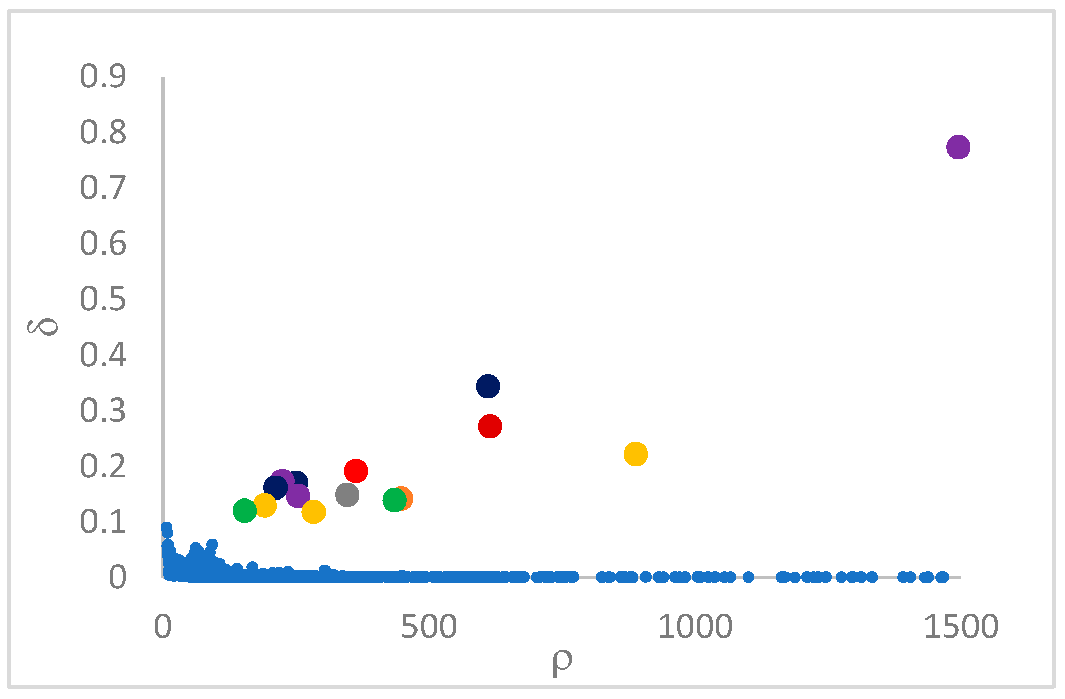
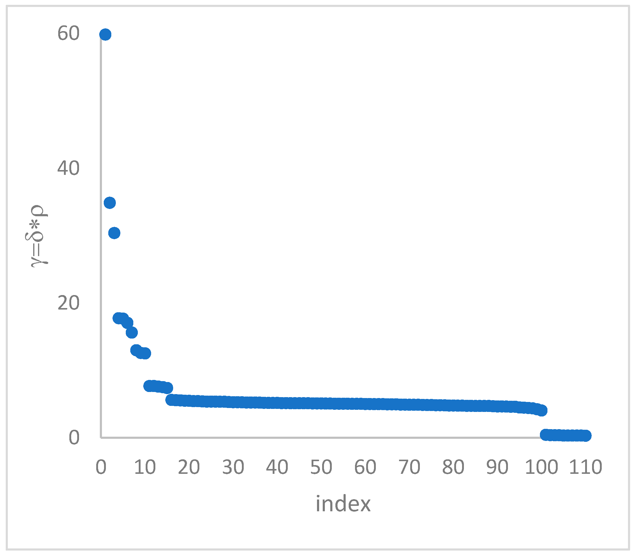
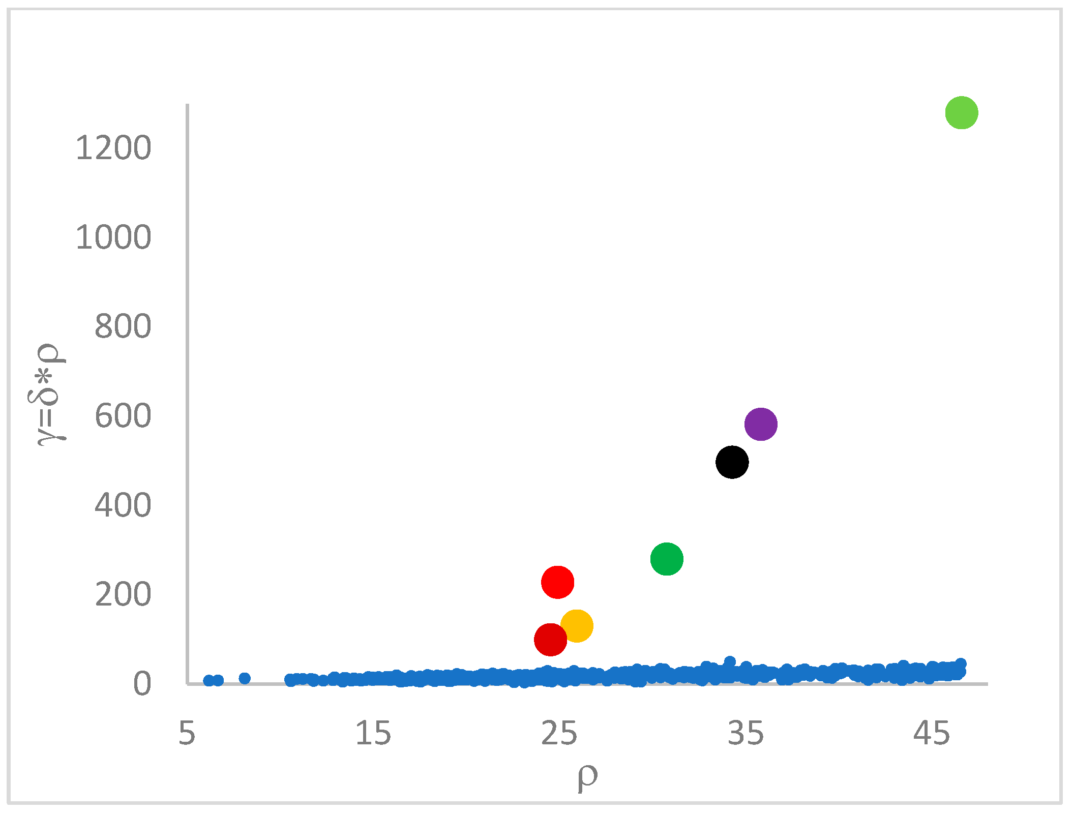
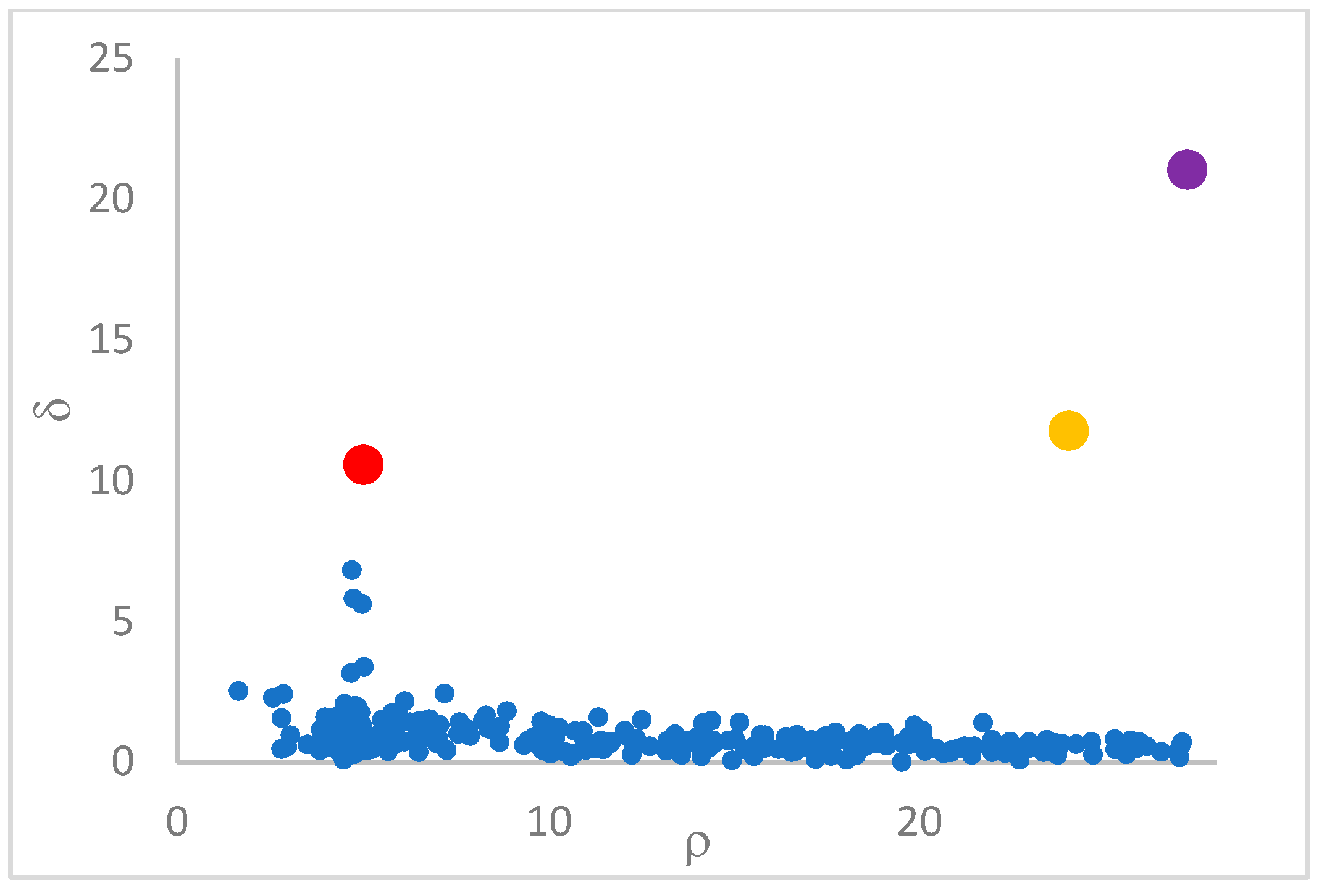
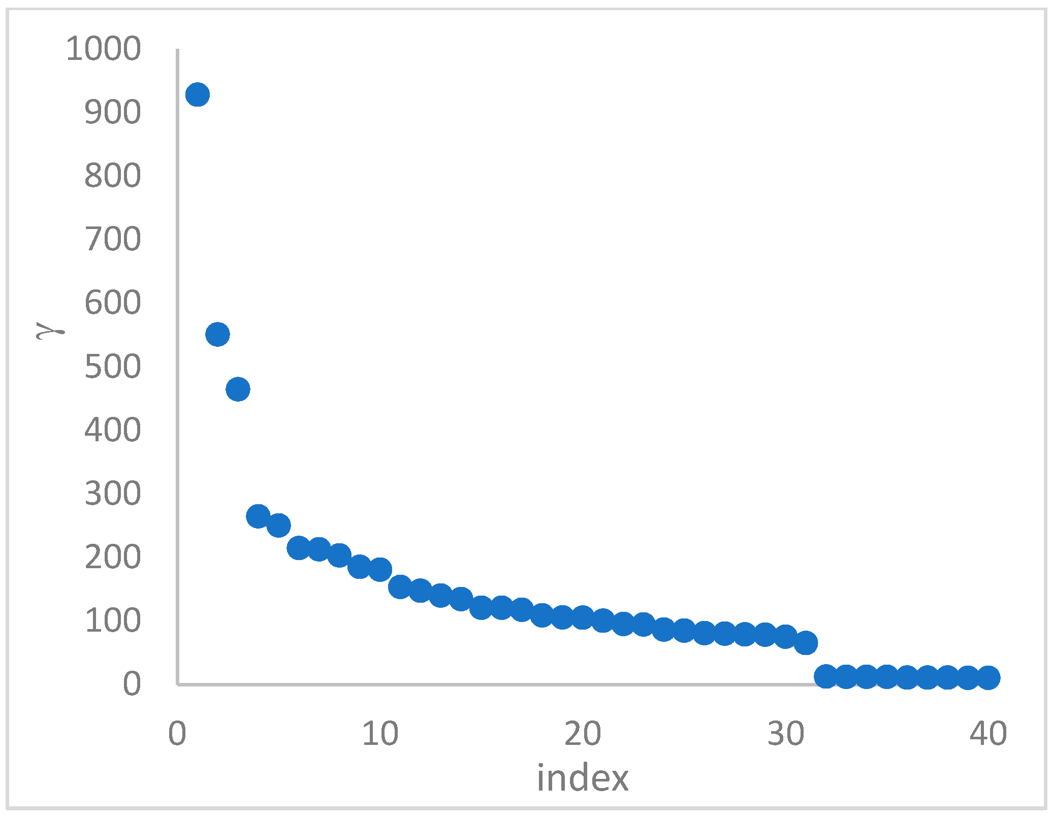
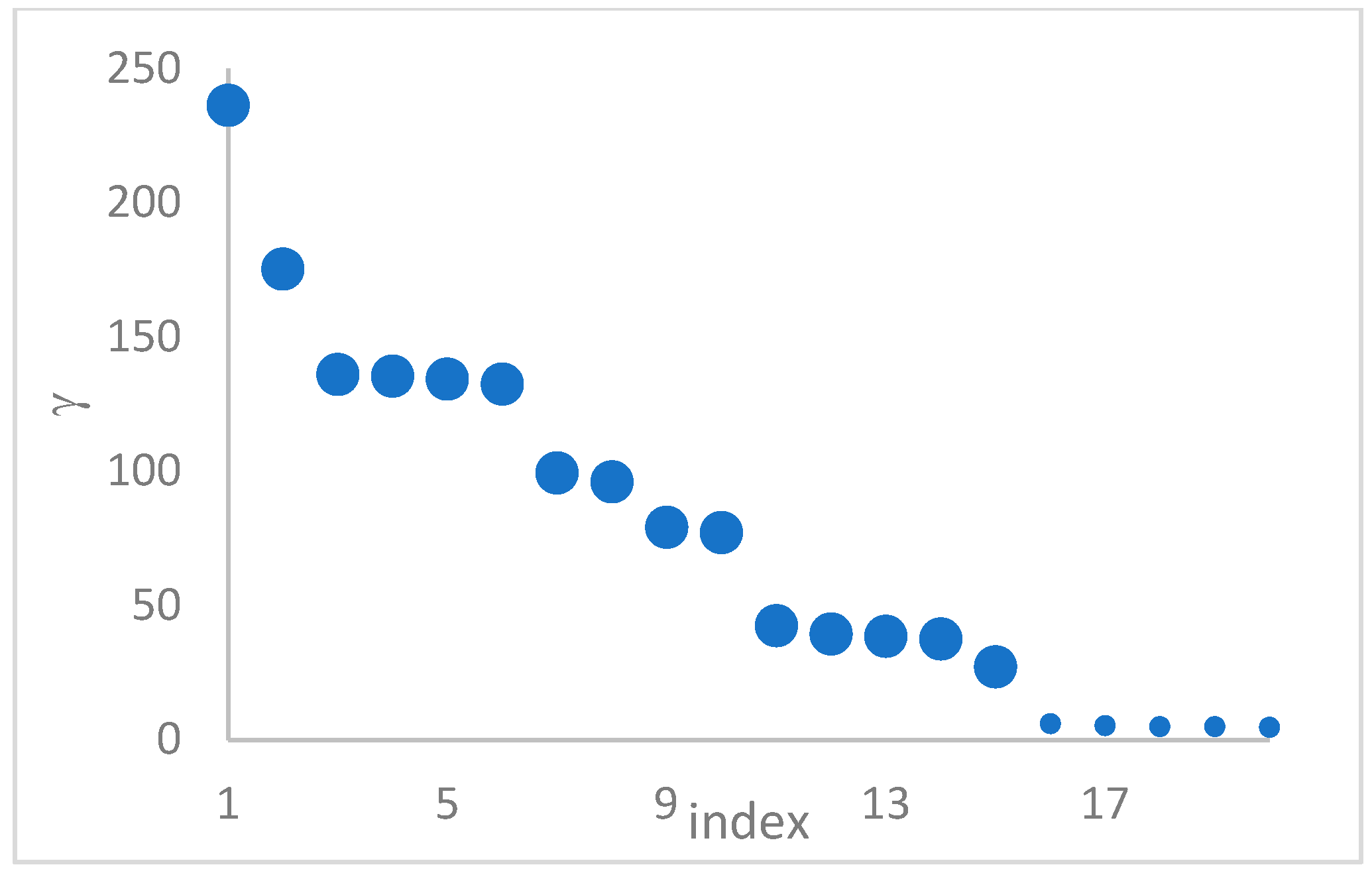
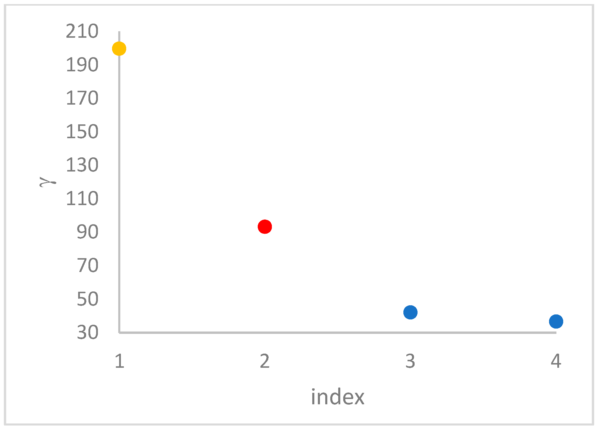
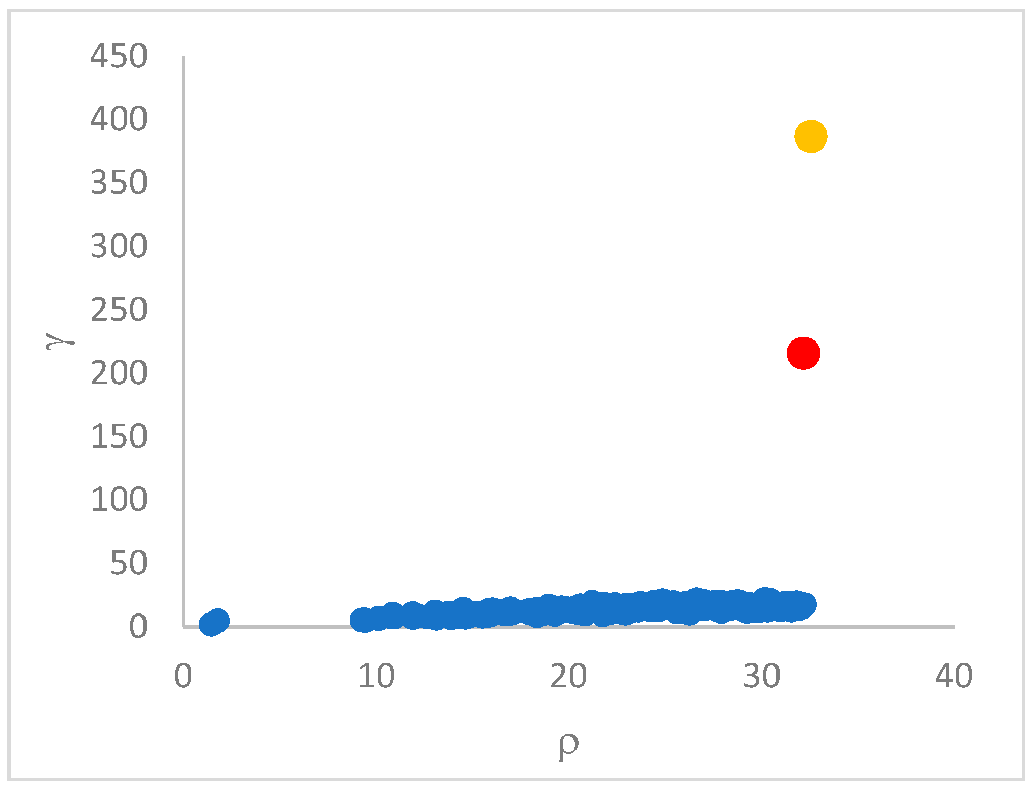
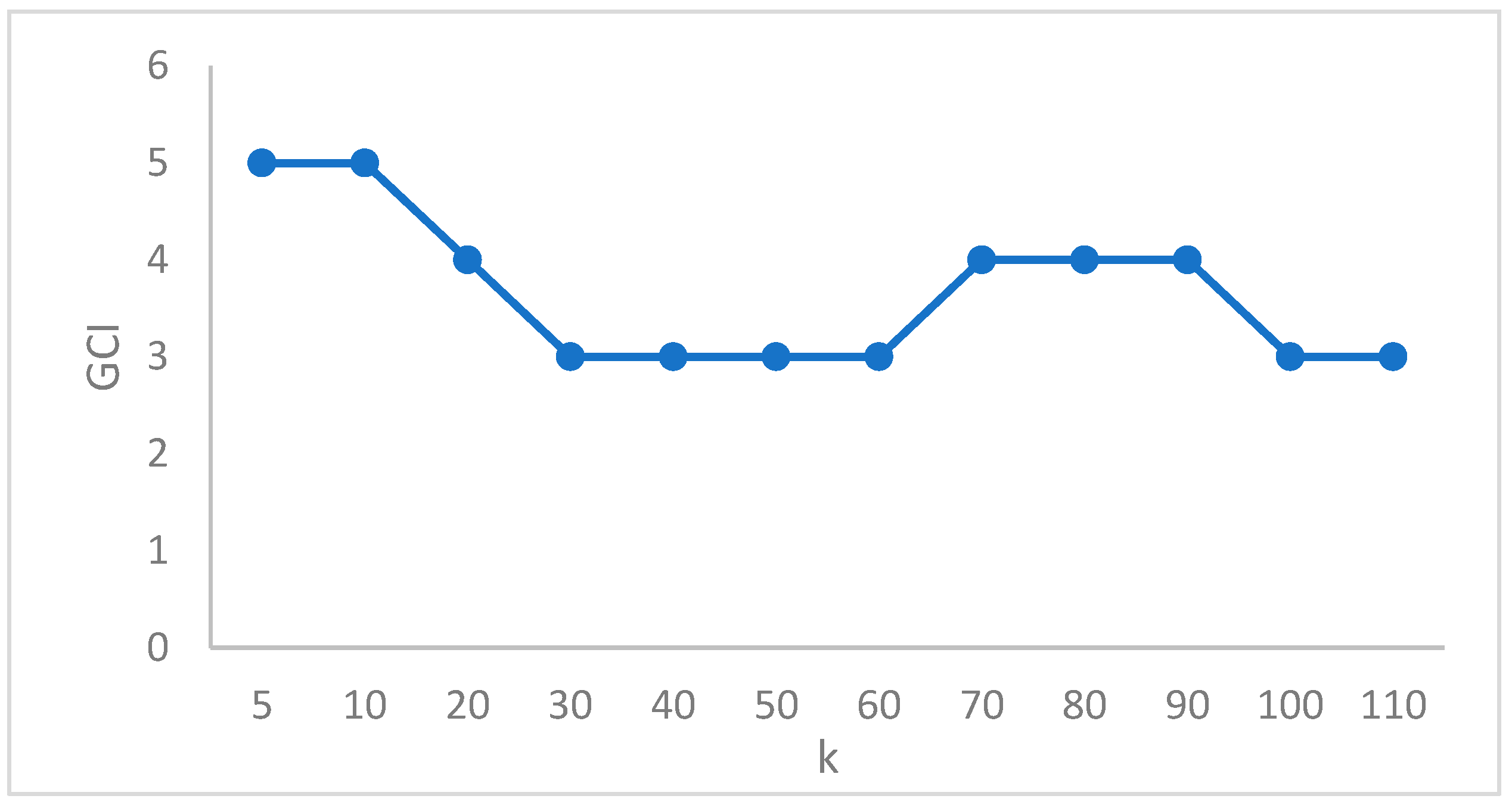
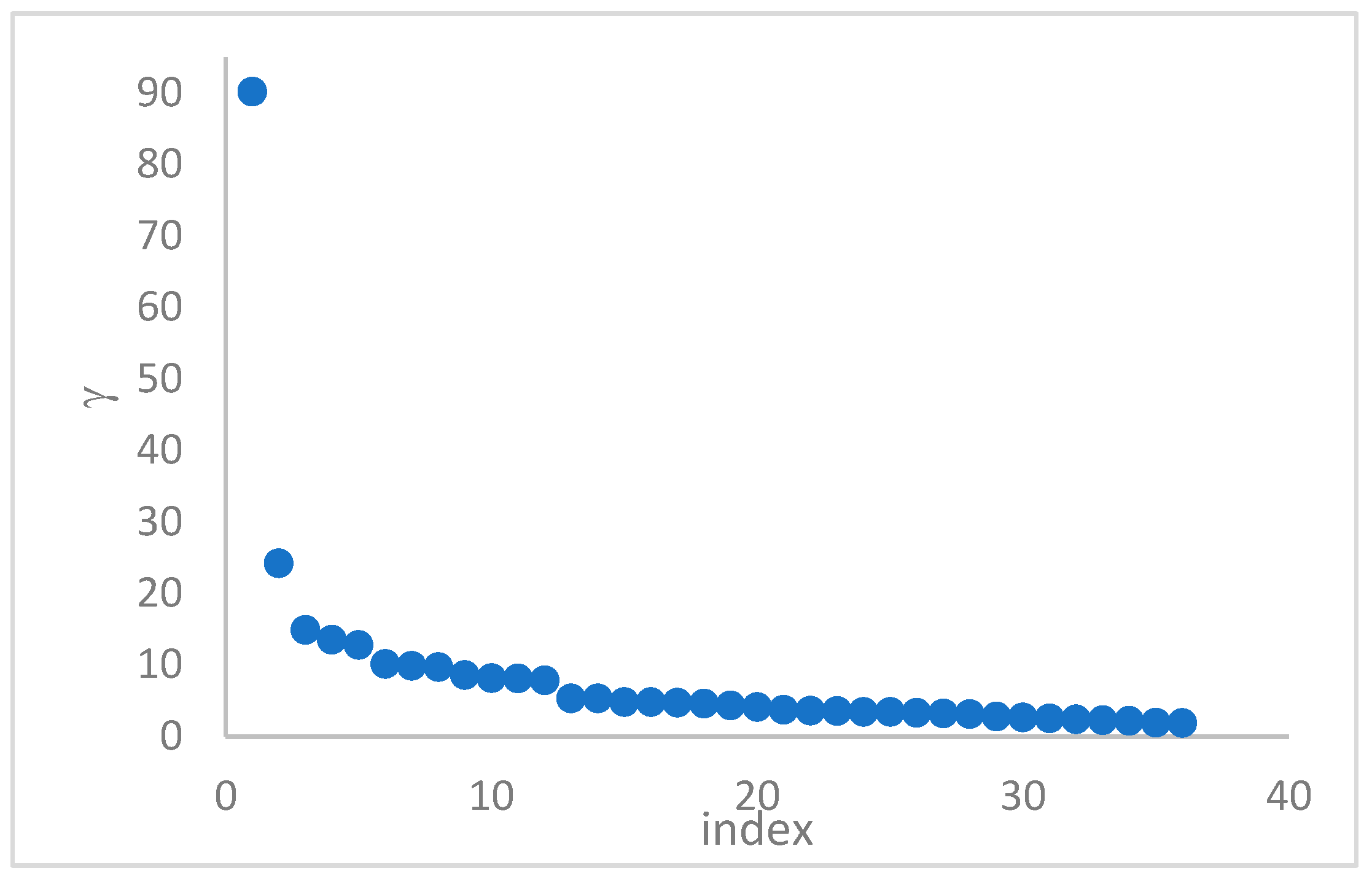
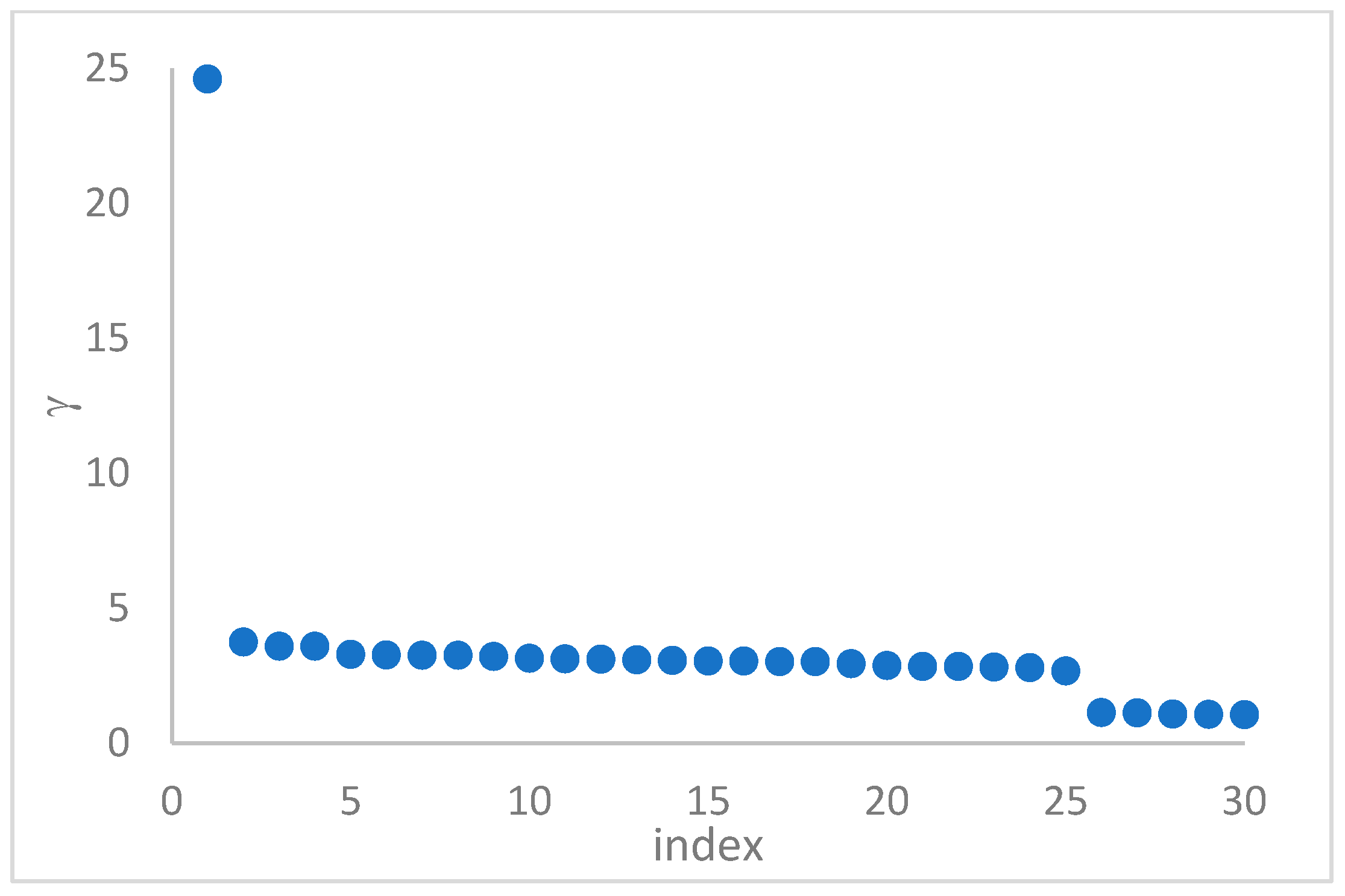
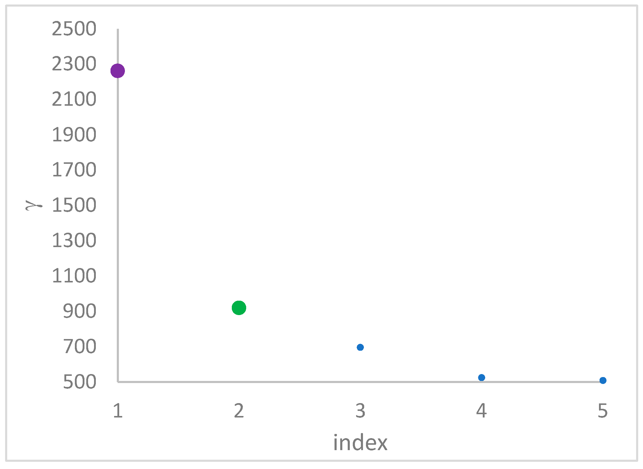
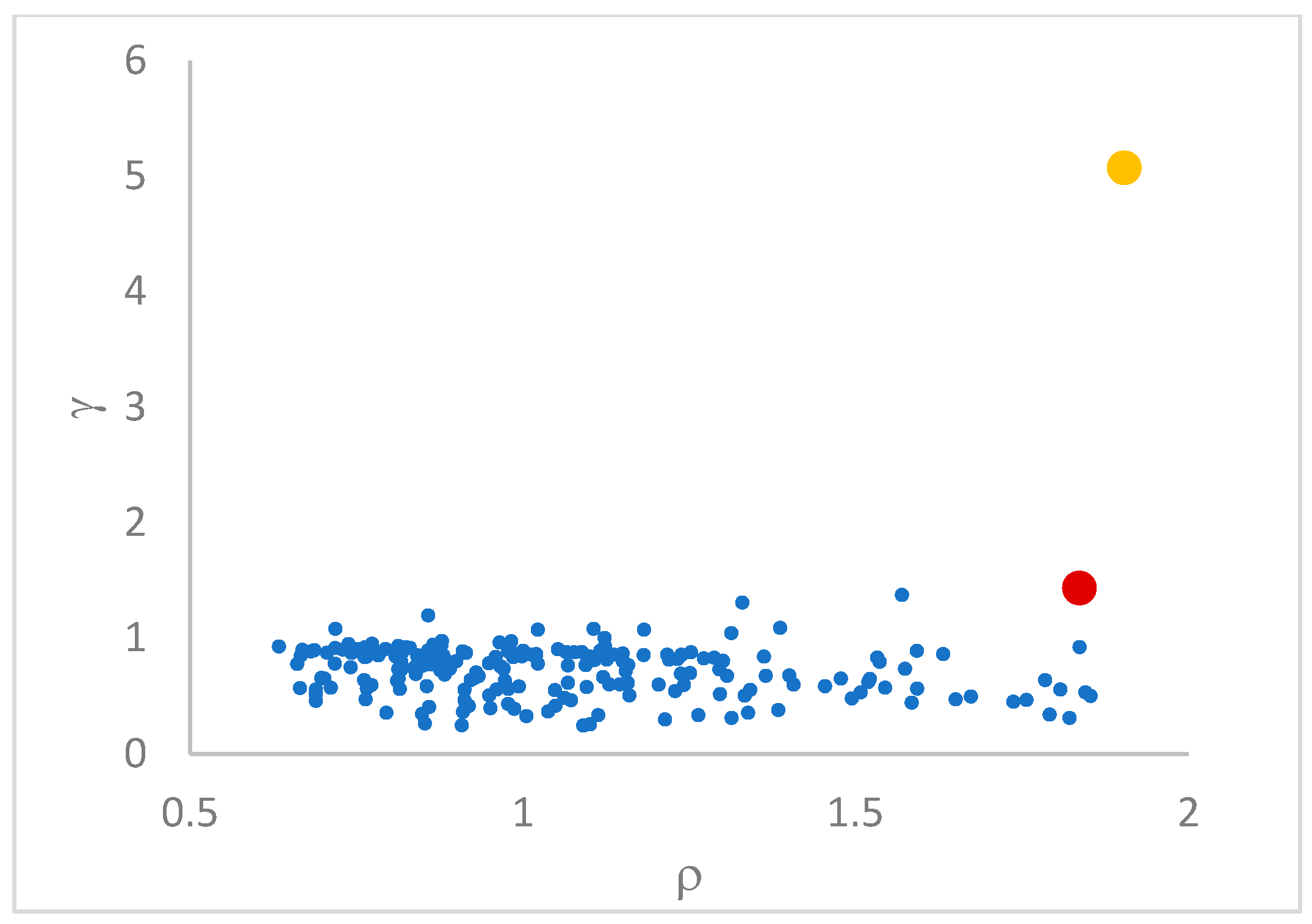
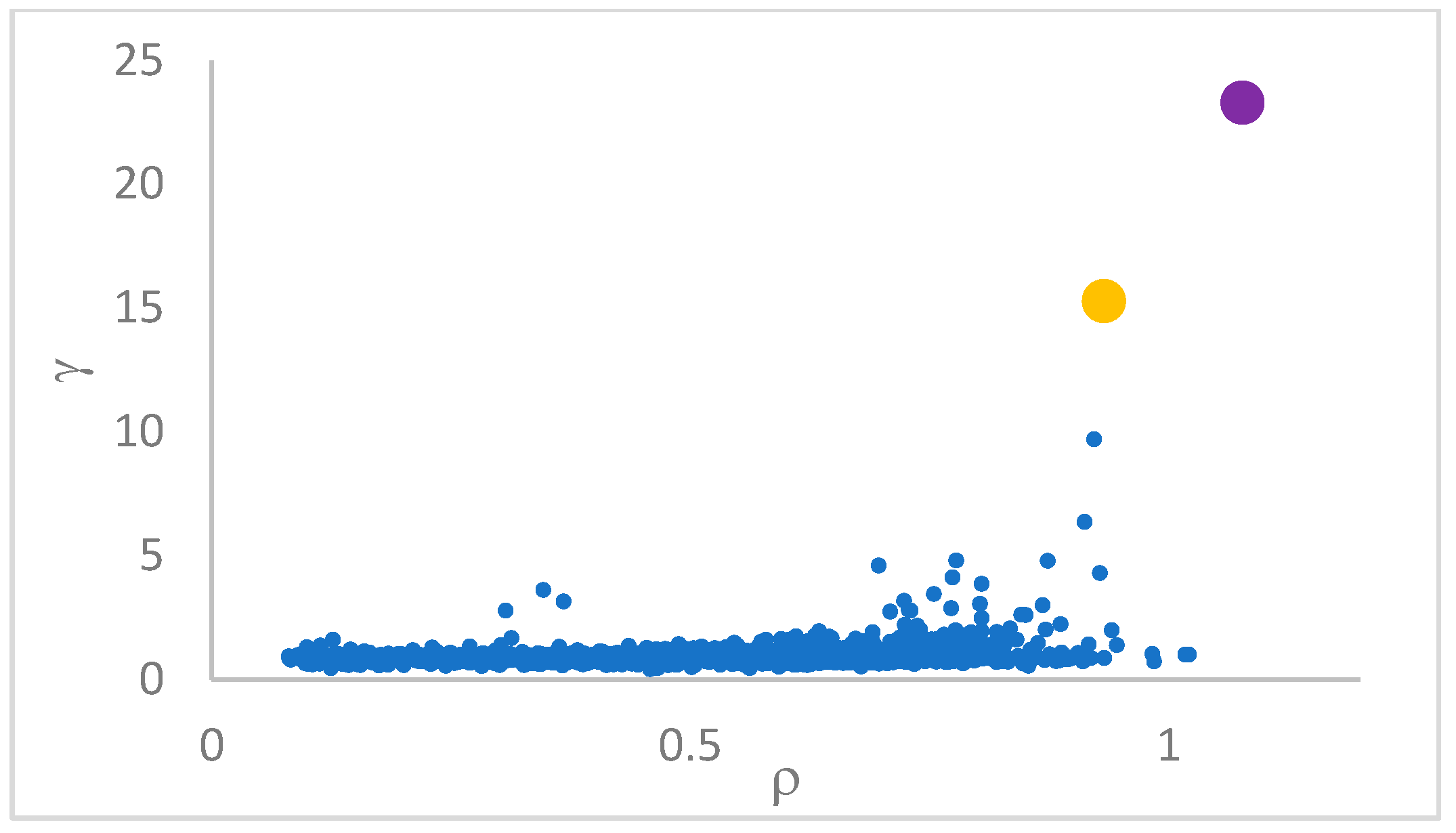
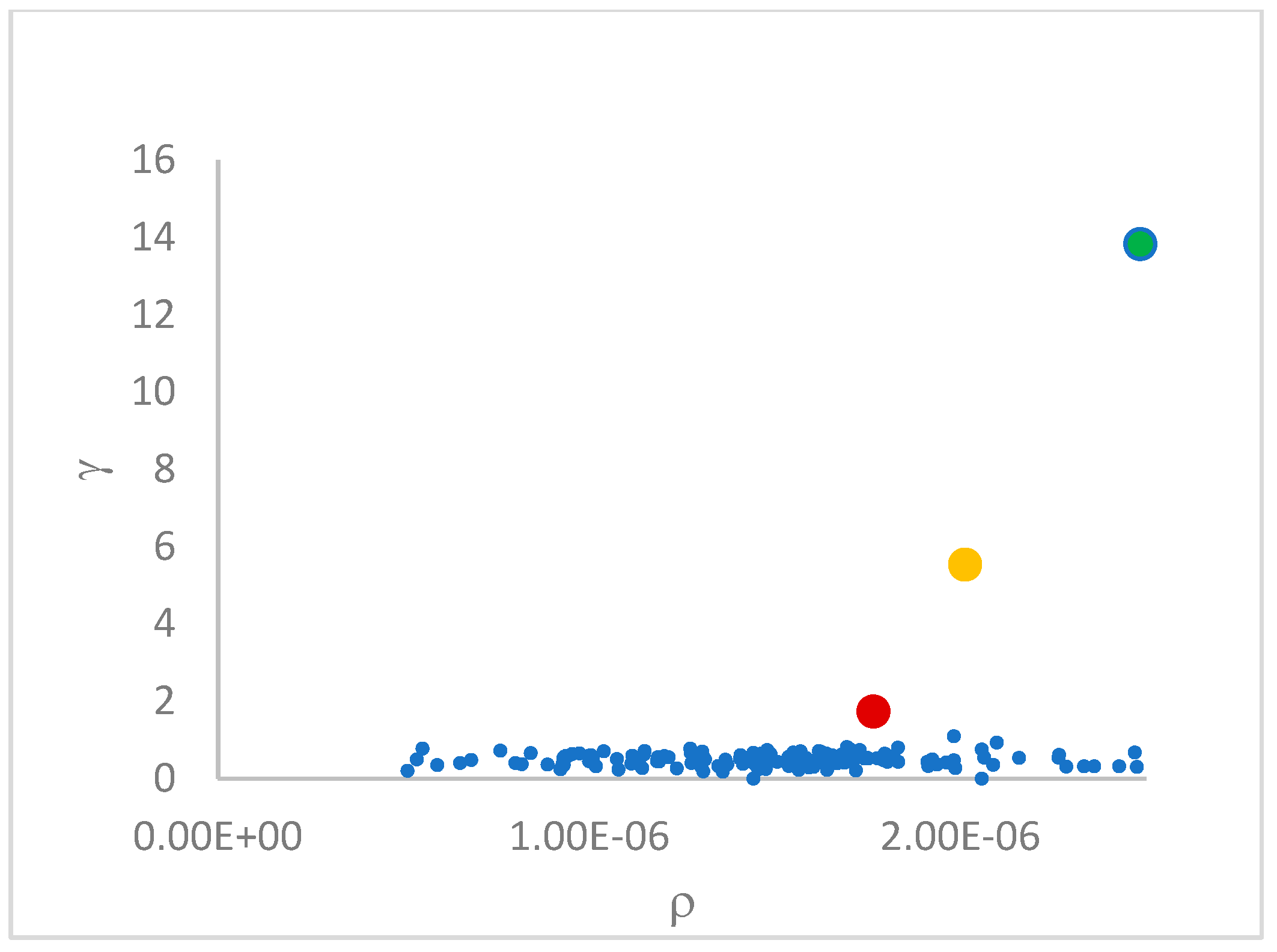
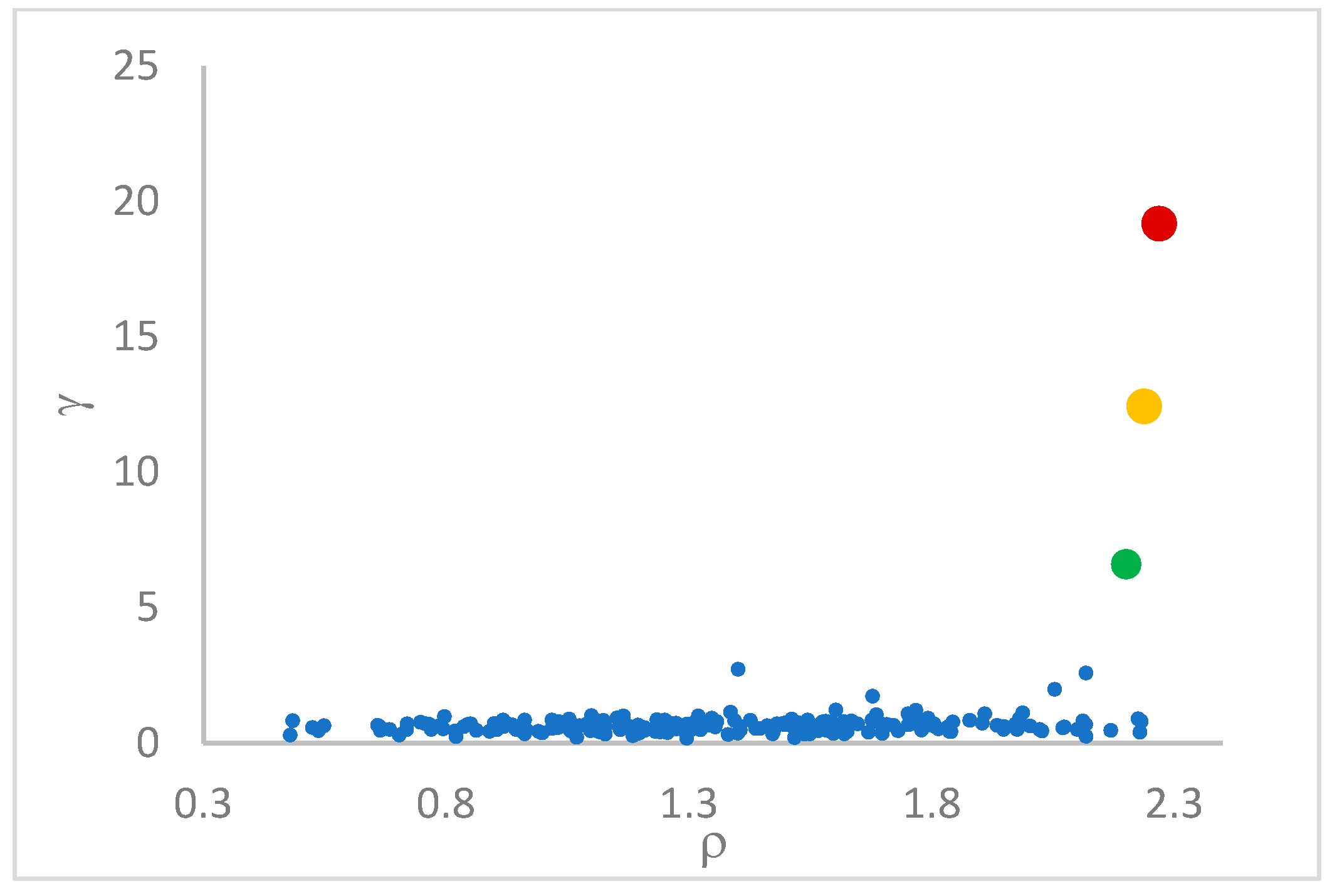
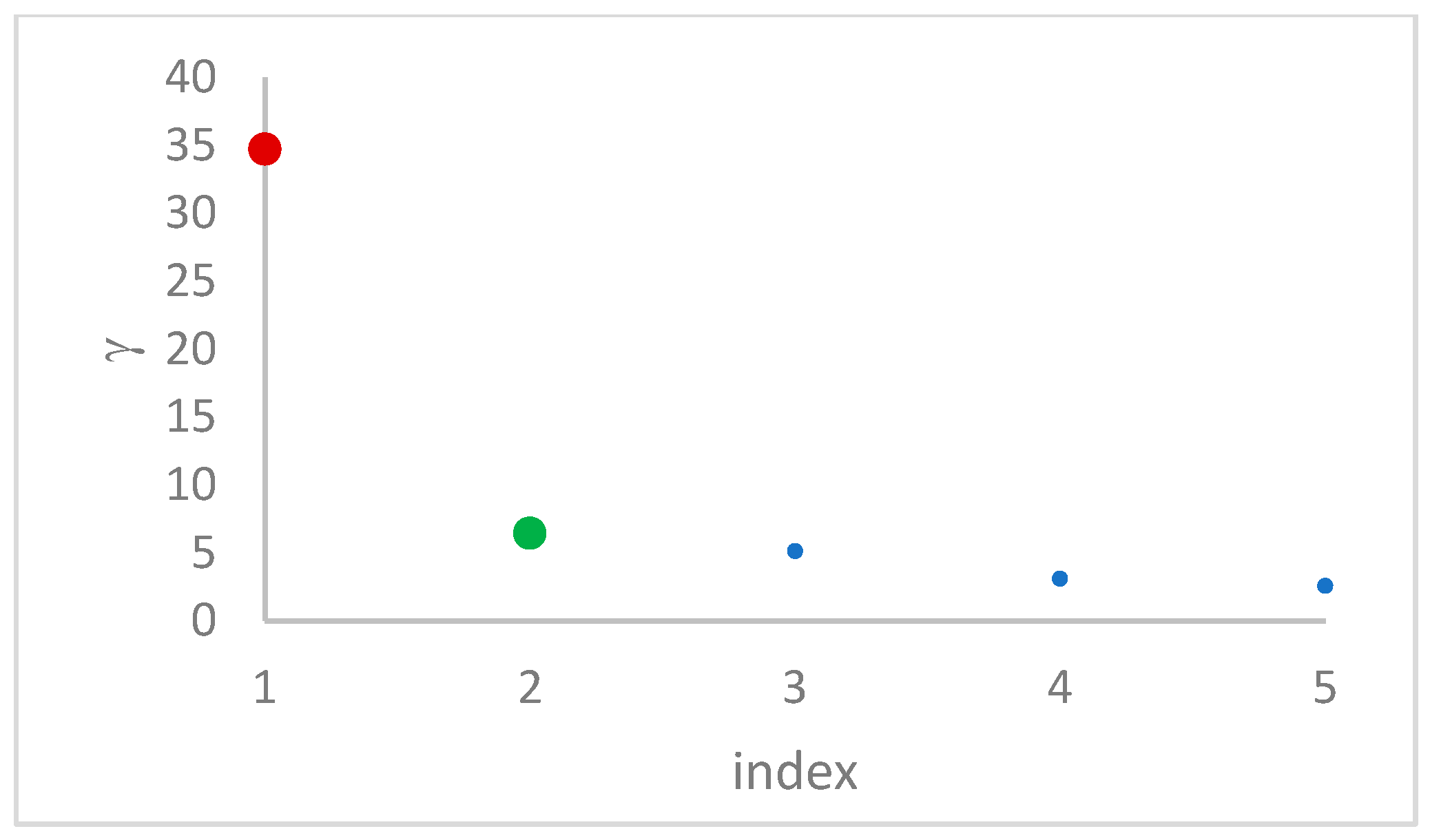
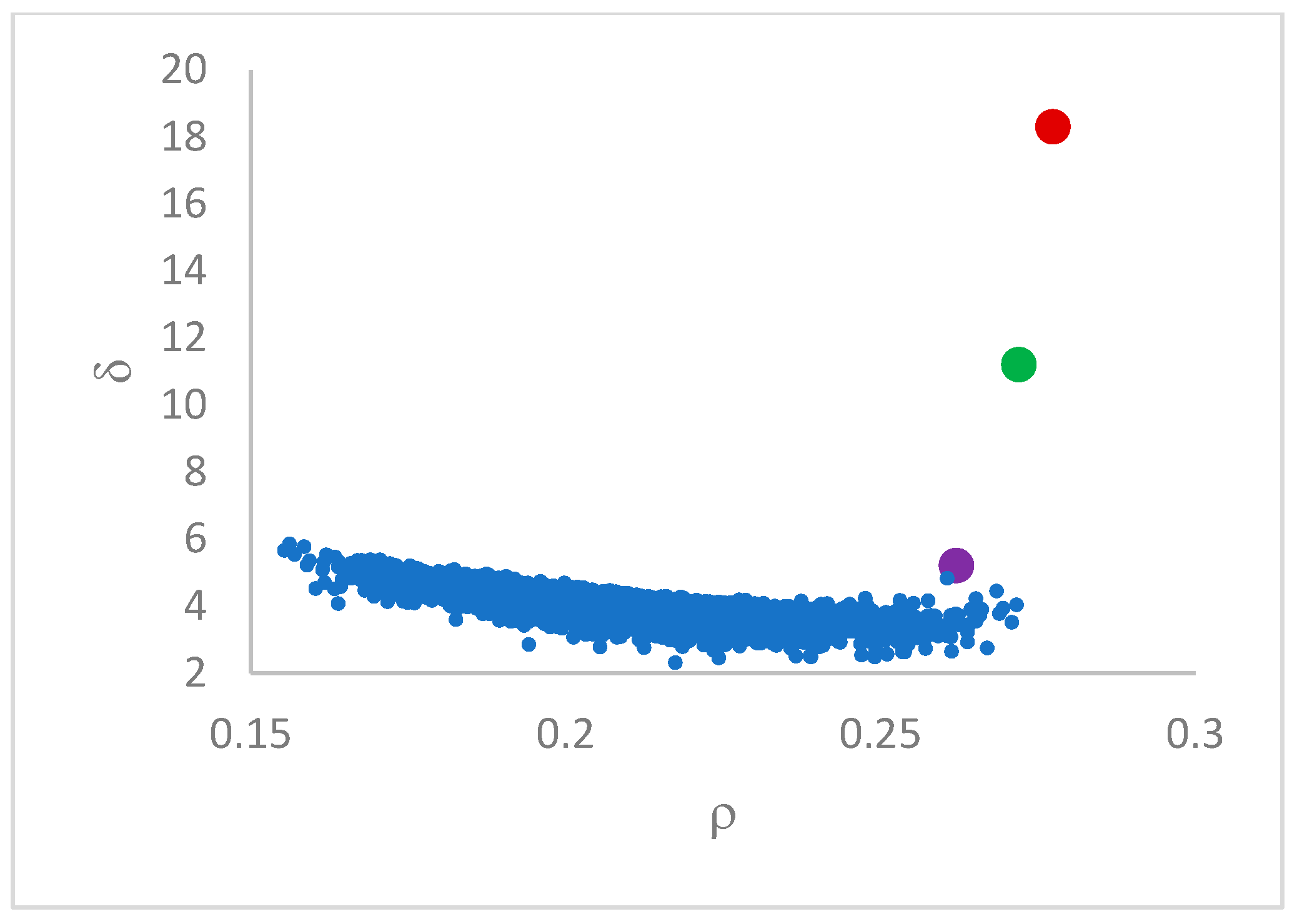
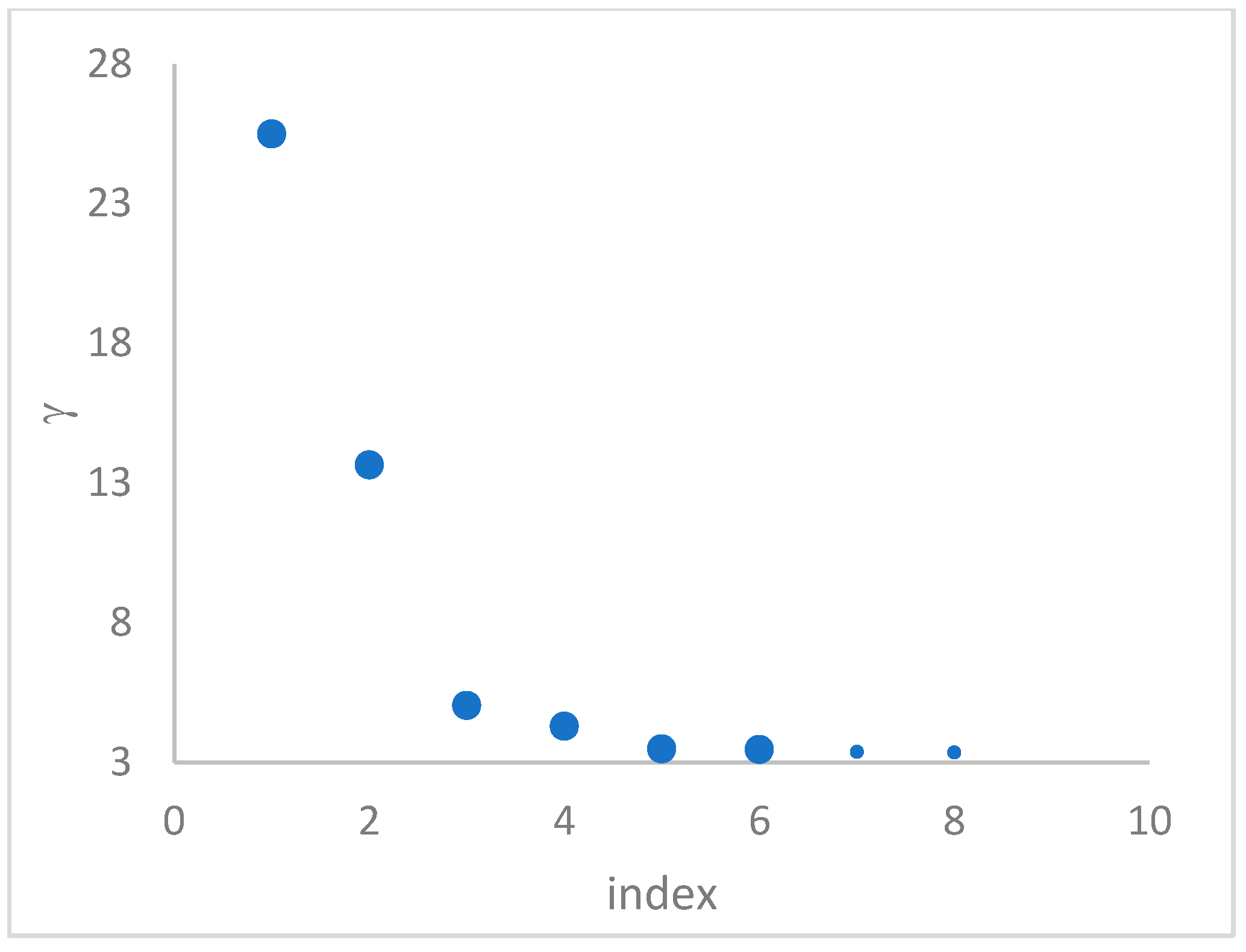
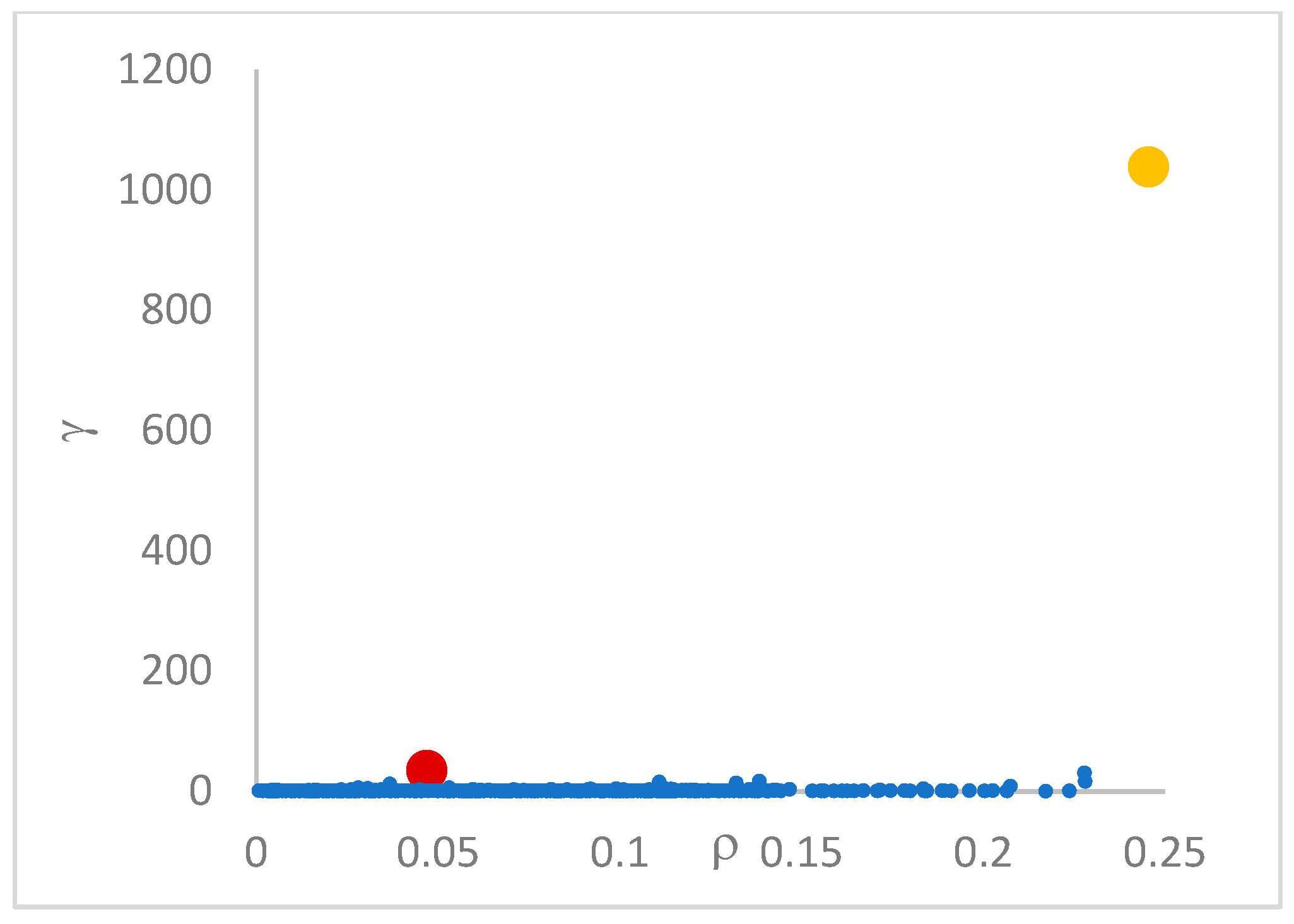
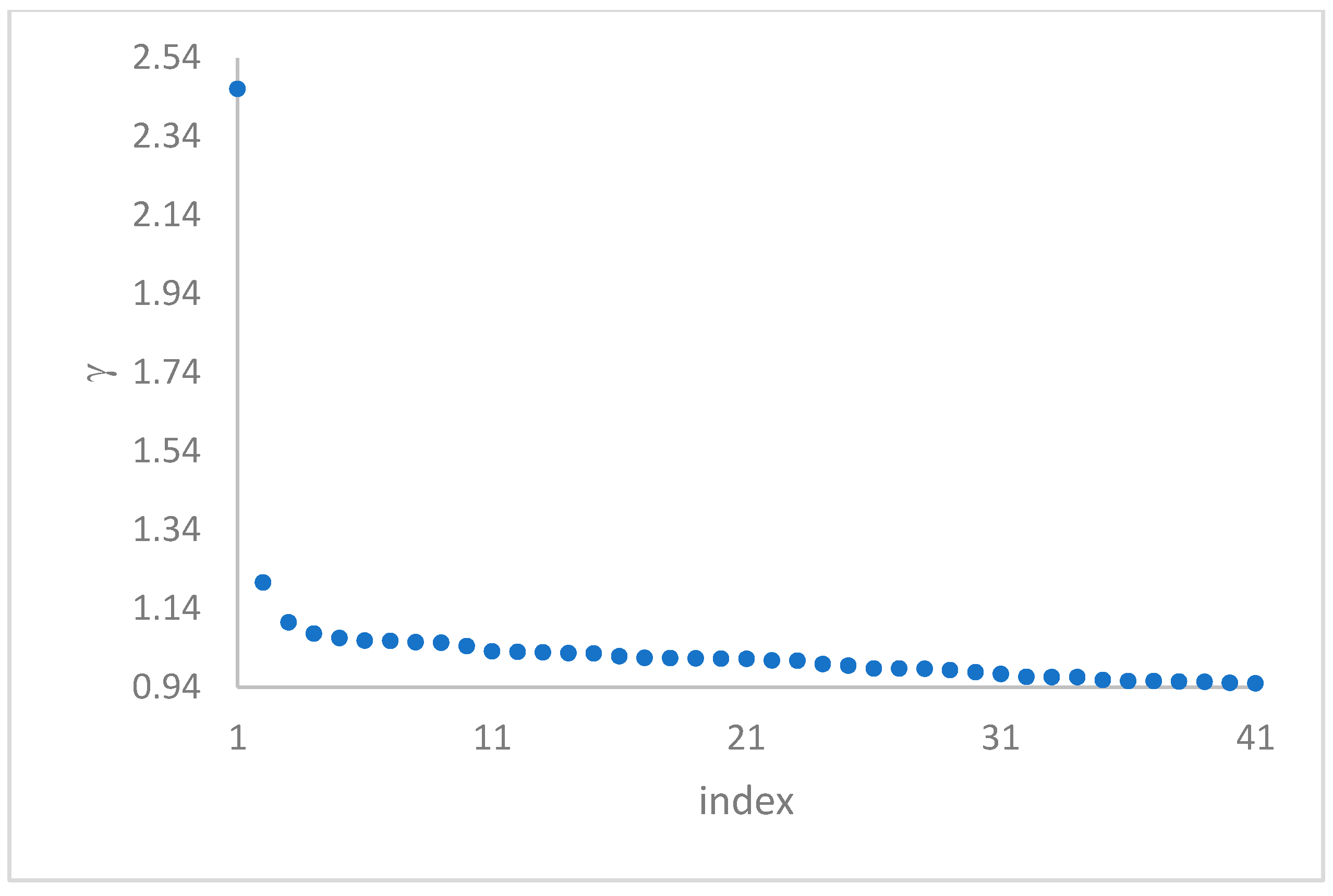
Unlike, e.g., K-Means [2,3], the number $K$ of centroids is not necessarily an input parameter for DP. The value of $K$ can, in many cases, be deducted by using the so-called decision graph, which depicts $\delta$ vs. $\rho$ or, better, $\gamma$ vs. $\rho$. Candidate centroids are expected to naturally emerge as points with the highest values of $\gamma$ in the decision graph. In the case the dataset is (logically) sorted by decreasing $\gamma$ values, as it is presented in this work, candidate centroids are the “first” points after which a sudden decrease (knee point) occurs for the $\gamma$ vs. dataset point indexes. However, the reading of centroids from the decision graph shows it is not always clear. In addition, some datasets come with a desired value of $K$, which suggests picking up the first $K$ points in the sorted dataset by decreasing $\gamma$.

A fundamental problem in DP is the definition of points’ density. In [12], the cutoff distance, $d_c$, is assumed, that is the common radius of a hyperball in the D-dimensional space, centered on any point, $x_i$. All the points that fall within $d_c$ establish the density $\rho \left(x_i\right)$:

$$\rho (x_i)=\sum _{j=1, j!=i}^N\chi \left(d\right(x_i,x_j)-d_c)$$

(1)

where $d(x_i,x_j)$ is the distance between $x_i$ and $x_j$, and $\chi \left(x\right)=1$ if $x<0$; otherwise, $\chi \left(x\right)=0$. In reality, in the implementation of DP, the authors of [12] used a Gaussian kernel instead for estimating the density:

$$\rho (x_i)=\sum _{j=1,j!=i}^N{e}^{-({\displaystyle \frac{{d(x_i,x_j)}^2}{{d_c}^2}})}$$

(2)

Such a choice [21] can be preferable because it avoids points having the same density as it may occur by counting with the cutoff distance. The following defines the delta feature of a point, $x_i$:

$$\delta (x_i)=\left\{\begin{array}{c}\max \left\{d\left(x_i,x_j\right), 1\le j\le N,j\ne i\right\}\mathit{if}\left(\rho \left(x_i\right)\ge \rho \left(x_j\right)\right)\forall j \\ \hfill \min \left\{d\left(x_i,x_j\right),1\le j\le N,j\ne i\right\} \forall j: \rho \left(x_i\right)<\rho \left(x_j\right) \hfill \end{array}\right.$$

(3)

This definition ensures that the point $x_i$ with the maximum density has its $\delta$ set to the maximum distance between $x_i$ and any other point in the dataset. Otherwise, $\delta \left(x_i\right)$ is set to the distance of the nearest point with a higher density.

Following the evaluation of $\rho \left(x_i\right)$, $\delta \left(x_i\right)$, and then of $\gamma \left(x_i\right)=\rho \left(x_i\right)\ast \delta \left(x_i\right)$, DP finalizes the clustering in a standard way. First, centroids are selected, according to the $\gamma$ values, and then they are assigned a label. After that, the labels of centroids are propagated to all the remaining points through the rule that a point acquires the label of its big brother.

DP can identify outliers by introducing a threshold, ${\rho }_b$, so that points that have a density less than ${\rho }_b$ are potential outliers or noise points. ${\rho }_b$ qualifies as the maximum density of points in the halo region of a cluster, which has points assigned to this cluster, but that are within the $d_c$ radius of points belonging to other clusters.

3. Development of the ParDP Algorithm

The design of ParDP was influenced by the basic DP work [12] and by work on kNN clustering [13,14,15,16,22]. The concepts of DP are inherited as ρ, δ, γ features of dataset points and the standard recursive clustering algorithm. Differences from DP are introduced in the way points’ density is evaluated.

Two kNN-based approaches are supported. As a preliminary task, the first $k$ distinct distances to the nearest neighbors are determined for each data point. Then the average of these $k$ distances is computed. In the first approach, similar to the work described in [16], the point density (mass divided by volume) is immediately estimated as the inverse of the average distance. In the second approach, the average distance is maintained in the data point as a local $d_c$. When all the dataset points have their local $d_c$ in place, a global $d_c$ is defined by sorting in ascending order all the local $d_c$ values and by extracting the median value as the common radius [12,22] for scanning the points’ density through a Gaussian kernel.

Both approaches naturally tend to limit the influence of outliers on the clustering process. For an outlier, the average of the first k nearest distances tends to be higher than the mean distance of non-outlier points. As a consequence, in the first approach, the density of the outlier is minimal, and the point has a lower probability of being chosen as a centroid. In the second approach, the choice of the median value of local $d_c$(s), paired with the use of a Gaussian kernel, again ensures that the density measure of the outlier point is very small.

The validity and efficacy of each supported kNN approach depend ultimately on the cluster shapes of the handled dataset, as confirmed experimentally (see later in this paper).

Algorithm 1 provides a pseudo-code of ParDP’s behavior. For some datasets, it can be helpful to preliminarily scale the dataset point coordinates, e.g., by a $min-max$ normalization, or dividing each coordinate by the maximum value of all features, and so forth. Steps such as pca(), kNN(), delta(), gamma, and clustering(), directly correspond to Java methods in the ParDP implementation.

Algorithm 1. Pseudo-code of basic ParDP operations.

Input: dataset X and (if there are any) ground truth centroids or partitions Scaling data if required pca() kNN() delta() gamma() if(decision graph is required)      Output: persist rho, delta and gamma values of the data points else      clustering()      Output: some accuracy measures of the achieved clustering solution

3.1. Step pca()

The following steps of principal component analysis [13,23] detect the most important coordinates of data points.

• Make each coordinate dimension (feature) have a 0 mean.
• Define the $D\times D$ covariance matrix $\mathsf{\Sigma }=X^t\ast X$ of the $N\times D$ matrix, $X$, associated with the dataset.
• Compute the eigenvalues ${\lambda }_j, 1\le j\le D,$ that is the diagonal elements, ${\mathsf{\Sigma }}_{j,j}$, of matrix $\mathsf{\Sigma }$ by the internal products:

  $${\lambda }_j={\sum }_{i=1}^N{X}_{j,i}^t\ast X_{i.j}$$

  (4)
• Extract the vector of $D$ eigenvalues $\left[{\lambda }_1,{\lambda }_2,\dots ,{\lambda }_D\right]$ from the matrix, $\mathsf{\Sigma }$.
• Sort by decreasing values the eigenvalues vector.
• Select the first $h, 1\le h\le D$ sorted eigenvalues that would ensure, e.g.,

  $${\displaystyle \frac{{\sum }_{j=1}^h{\lambda }_j}{{\sum }_{j=1}^D{\lambda }_j}}\ge 0.99$$

  (5)

Practically, only the indexes of the most important coordinates (those having higher eigenvalues) are retained during the sorting of the eigenvalues. Such indexes are then used when computing the Euclidean distance between two data points.

3.2. Step kNN()

This step realizes the two approaches to the density evaluation of ParDP. A global boolean $CUTOFF$ parameter permits kNN() to adapt its behavior to one of the two approaches. The value of the parameter $k$ is important. Algorithm 1 is supposed to be repeated for different values of $k$, whose “best” value must be tuned to the dataset. For example, several datasets used in the experiments reported in this paper were investigated by using the range [5…200] for $k$. The effects of a particular value of $k$ on the clustering can be checked on the decision graph or by observing some clustering measures (see later in this paper). The execution of the kNN() step (see also Section 2) assigns to each point $x_i$ its estimated density but also the maximal distance of $x_i$ from any other point in the dataset. Such information is used by the subsequent delta() step. For each value of $k$, the kNN() step costs $O\left(N^2\right)$ to compute all the pairwise distances of points. To this cost, the heap sorting cost, $O\left(NlogN\right)$, of the dataset by ascending local cutoff distances of data points is added if the cutoff approach of ParDP is chosen. The dominant $O\left(N^2\right)$ cost is smoothed by using Java parallel streams (see Section 3.6).

3.3. Step delta()

This step is responsible for assigning the information about big brother into each data point. Toward this goal, first, the dataset is sorted by decreasing values of the points’ density. Then, for each point, $x_i$, the points $x_j$ located at its left in the ordered sequence of data points are considered, and the distance, $d(x_i,x_j)$, is evaluated. Finally, the identity (index) and distance of point $x_j$ nearest to $x_i$ are stored in $x_i$ as its big brother. In the case of point $x_1$ that has the maximal density, its big brother is set, by convention, to the point that has the maximal distance from $x_1$, as determined in the kNN() step.

In this step, dataset points are sorted by descending values of the density feature. In the next gamma() step, the dataset has to be sorted by decreasing values of the gamma feature of the dataset points. To cope with these conflicting issues and also to maintain the integrity of some fundamental information, like the index of the big brother of a point, ParDP behaves as follows. In no case are points moved within the dataset during a sorting operation. Rather, an $index$ data structure is used that indirectly references the points of the dataset. Therefore, the effects of sorting are reflected by the references kept in the $index$. At the time of fixing the identity of the big brother of a point, $x_i$, the absolute, never-changing physical index (that each point stores in itself) of the big brother (iDelta) and its distance (delta) are stored in $x_i$. The technique makes it possible to sort, at different times and according to different ordering criteria, the dataset points.

The delta() step mainly costs $O\left(NlogN\right)$ for heap sorting the dataset by the descending density of the points, which includes the $O\left(N\right)$ cost for searching the big brother of each point.

3.4. Step gamma()

This step sorts the dataset by decreasing $gamma$ $\left(\mathsf{\gamma }\right)$ values, that is the product of ρ (density) per $\delta$(delta or distance to big brother) of data points. Such ordering is a key to inferring the number $K$ of clusters suited for a dataset or to assessing the validity of the a priori known value of $K$. All these activities can be carried out on the decision graph. Three equivalent types of decision graphs can be exploited: $\delta$ vs. ρ, $\mathsf{\gamma }$ vs. ρ, or $\gamma$ vs. (sorted dataset point) index.

The gamma() step has the $O\left(NlogN\right)$ cost for heap sorting the dataset by the descending gamma values of points.

3.5. Step clustering()

This step selects the first $K$ points in the dataset, sorted by decreasing gamma values, as centroids (see Section 3.4); assigns to each centroid a label identical to its index; and then proceeds with the final clustering as in the basic DP algorithm (see Section 2) [12]. In particular, each point is assigned the label (cluster) of its big brother. In the case the big brother is still unassigned, the procedure continues, recursively, by moving to its big brother and so forth until a centroid or an already assigned big brother is found from which its label is propagated back to all the points in the recursion return path.

The clustering step() costs about $O\left(N\right).$ Overall, the ParDP execution costs $O\left(N^2\right)$.

3.6. Java Implementation Issues

The power and flexibility of ParDP derive from its implementation, which is based on Java parallel streams and lambda expressions [19]. The same parallel and functional programming mechanisms were previously successfully applied, for example, to improve the execution of K-Means [4] and Random Swap [9,11]. A stream is a view of a data collection (e.g., an array like the dataset managed by ParDP) making it possible to express element operations functionally by lambda expressions. A parallel stream allows for the underlying fork/join mechanism to be exploited, which splits the data into multiple segments and processes segments by separate threads. Finally, it combines the partial results generated by the worker threads. A key benefit of the parallel stream concerns taking advantage of the high-performance computing environment provided by a multi/many-core machine, where lock-free parallelism is used, requiring lambda expressions of not modifying shared data.

The concise and elegant programming style ensured by parallel streams and lambda expressions is exemplified in Algorithm 2, where the non-cutoff-based approach of ParDP for predicting the points’ density is shown. First, a stream is opened on the dataset to process points in parallel. Computation is embedded in the map() operation, which works on a stream, transforms it, and returns a new stream. map() is an intermediate operation. The execution of the various map() operations is triggered by a terminal operation, like forEach(). Each map() receives a UnaryOperator<DataPoint> object whose apply() method is formulated by a lambda expression, which receives a point, p; transforms it (p is purposely mapped); and, finally, returns p. A key point of the realization in Algorithm 2 is that each point, p, only modifies itself (the rho and dMax fields of p are modified). Absolutely no other changes are made to the shared data. The overall programming style only specifies what to do. The parallel organization and execution of the code is delegated to the built-in fork/join control structure [19].

Algorithm 2. An excerpt of the kNN() method for the non-cutoff approach to density

… Stream<DataPoint> pStream = Stream.of(dataset); if(PARALLEL) pStream = pStream.parallel(); pStream     .map(p->{        //detect distances to the first distinct k nearest neighbors of p        double[] dkNN = new double[k];        for(int j = 0; j < k; ++j) dkNN[j] = Double.MAX_VALUE;        double dMax = Double.MIN_VALUE; //maximal distance of p to any other point        for(int i = 0; i < N; ++i) {                 if(i! = p.getID()) {                            double d = p.distance(dataset[i]);                            if(d > dMax) dMax = d;                            int j = 0;                            while(j < k) {                                  if(d < dkNN[j]) {                                             //right shift from j to k − 1                                             for(int h = k − 2; h >= j; --h) dkNN[h + 1] = dkNN[h];                                             dkNN[j] = d; break;                                  }                                  else if(d == dkNN[j]) break;                                 j++;                            }                 }       }       double ad = 0;       for(int j = 0; j < k; ++j) ad = ad + dkNN[j];       p.setRho(k/ad); //inverse of average kNN distances       p.setDMax(dMax);       return p;     })    .forEach(p->{}); //trigger of map computations

Parallel streams are systematically adopted in ParDP, anywhere parallelism can be exploited. For example, in the delta() step of Algorithm 1, first the dataset is sorted by decreasing density values, then a parallel stream is opened and used to determine the big brother of each point, p. Parallel streams are also used for computing internal or external clustering accuracy measures.

4. Clustering Accuracy Measures

The validity or quality of a clustering solution generated by a given algorithm can be measured by some internal or external indexes [9,24]. Internal indexes are related to the internal composition of points of clusters. Two well-known indexes in this class are the Sum-of-Squared Errors ($SSE$) and the Silhouette coefficient ($SI$) [11,25]. The $SSE$ reveals how close the points assigned to the various clusters $[C_1,C_2,\dots ,C_K]$ are to their relevant centroids $[{\mu }_1,{\mu }_2,\dots ,{\mu }_K]$:

$$SSE={\sum }_{j=1}^K{\sum }_{x_i\in C_j}{d(x_i,{\mu }_j)}^2$$

(6)

The Silhouette coefficient, $SI$, is a joint measure of the internal compactness (cohesion) of clusters and their separation, which, in turn, is related to the overlapping degree of the clusters. The $SI$ of a point, $x_i$, is computed as:

$${SI}_{x_i}={\displaystyle \frac{{b_{x_i}-a}_{x_i}}{\max (b_{x_i},a_{x_i})}}$$

(7)

where $a_{x_i}$ is the average distance of $x_i$ from the remaining points of the belonging cluster, and $b_{x_i}$ is the minimal average distance of $x_i$ to all the points of other clusters. The overall $SI$ is then defined as:

$$SI={\displaystyle \frac{1}{N}}{\sum }_{i=1}^N{SI}_{x_i}$$

(8)

$SI$ ranges in $[-1, 1]$. A value close to 1 mirrors the well-separation of clusters in the achieved solution. A value close to 0 expresses the high overlapping of the clusters. A value that tends to −1 indicates wrong clustering.

It is worth noting that $SSE$ or the $SI$ can directly be used as the optimization function in K-Means, Random Swap, and similar algorithms. DP, though, is not driven directly by the optimization of such internal indexes. DP, instead, is better evaluated by the use of external measures of the similarity (or dissimilarity) degree of two solutions: $S^1$ and $S^2$. Each solution is composed of a vector of $K$ centroids and a vector of $K$ partitions, which are sets of points (indexes) assigned to the same cluster. Labels are the integers in [1..$K$]. The number $K$ can be different in the two solutions, although it is usually the same value (assumed in the following). In some cases, one of the two solutions can be a ground truth ($GT$) correct (“optimal”) solution. $GT$ can be generated by the designer of a synthetic or benchmark dataset to allow the assessment of the accuracy of a particular solution ($C$) predicted by a clustering algorithm. In other cases, the ground truth can be a “golden solution” generated by an assumed correct algorithm. A correct solution can be available as a collection of ground truth centroids ($GTC$) or ground truth partition ($GTP$) labels assigned to all the points, e.g., of a real-world dataset. $GTP$ mirrors the best partition of the points into clusters.

External quality indexes include the Cluster Index ($CI$) [26], the Generalized Cluster Index ($GCI$) [27], the Adjusted Rand Index ($ARI$) [24], the accuracy index ($ACC$) [28], and the Normalized Mutual Information (NMI) index [24]. External indexes can be pair-matching or set-matching measures. In pair-matching measures, the centroids of the two solutions can be mapped onto each other and, possibly, in the two directions: $S^1\to S^2$ and $S^2\to S^1$. Alternatively, pairs of points can be matched among the clusters (partitions) of the two solutions. In set-matching measures, partitions are mapped onto each other between the two solutions.

The Cluster Index ($CI$) maps each centroid of $S^1$ to the nearest one in $S^2$, according to the Euclidean distance. The number of orphans in $S^2$, that is the number of centroids upon which no centroid of $S^1$ is mapped, is then counted. $CI$ continues by also mapping centroids of $S^2$ onto $S^1$ and by counting the resultant orphans in $S^1$. The maximal number of orphans in the two directions of mapping defines the value of the $CI$. $CI$ ranges from 0 to $K$. The case where $CI=0$ indicates $S^1$ is structurally correct to $S^2$. A $CI>0$ mirrors the number of wrongly detected clusters/centroids. $CI$ can be practically applied to measure the similarity between the centroids of a predicted clustering solution and the ground truth centroids ($GTC$) available for the dataset. The set-matching-based Generalized Cluster Index ($GCI$) extends $CI$ to the cases where the partitions of a particular solution are mapped to the ground truth partitions ($GTP$) available for a dataset. In this case, the Jaccard distance [11,27] between two partitions (sets of points) can be exploited for establishing the nearness:

$$Jd=1-{\displaystyle \frac{\left|P_1\cap P_2\right|}{\left|P_1\cup P_2\right|}}$$

(9)

The pair-matching-based $ARI$ index [24,29] maps pairs of points from $S^1\to S^2$, practically, from detected to ground truth clusters. It is defined as:

$$ARI={\displaystyle \frac{2(ad-bc)}{\left(a+b\right)\left(b+d\right)+(a+c)(c+d)}}$$

(10)

where $a$ counts the number of pairs of points that belong to the same cluster in $S^1$ and the same cluster in $S^2$; $b$ counts the number of pairs that are in the same cluster in $S^1$ but in different clusters in $S^2$; $c$ counts the number of pairs that are in distinct clusters in $S^1$ but in the same cluster in $S^2$; finally, $d$ counts the number of pairs that belong to different clusters in $S^1$ and different clusters in $S^2$. The four quantities can be computed from the contingency matrix $S^1\times S^2$ [24]. The $ARI$ index ranges in [0..1]. Good clustering is mirrored by an $ARI$ value close to 1.

The accuracy index is defined as:

$$ACC={\displaystyle \frac{1}{N}}{\sum }_{i=1}^N\delta (S_{x_i}^2,map(S_{x_i}^1\left)\right)$$

(11)

where $\delta$ is the Kronechker operator which returns 1 if the two arguments are equals, 0 otherwise. The notation $S_{x_i}^j$ indicates the cluster (partition) of the solution $S^j$ to which the data point $x_i$ is assigned. The function $map\left(S_{x_i}^1\right)$ maps the partition in $S^1$ containing $x_i$ to a partition of $S^2$. In this work, the set-matching-based bi-directional definition of the $ACC$ proposed in [28] is adopted. The measure exploits the contingency matrix separately built in the two directions of mapping. $ACC$ ranges in [0..1], where values close to 1 mirror good clustering.

The NMI index is an information theoretic measure that can be computed using the contingency matrix [24] again. It is defined in terms of the Mutual Information (MI) and the Entropy (H) measures of the partitions of the two solutions, $S^1$ and $S^2$, to be compared.

$$MI={\sum }_{i=1}^K{\sum }_{j=1}^K{\displaystyle \frac{\left|S_i^1\cap S_j^2\right|}{N}}log{\displaystyle \frac{N\ast \left|S_i^1\cap S_j^2\right|}{\left|S_i^1\right|\ast \left|S_j^2\right|}}$$

(12)

where 0*log0 is assumed to be 0. The quantity $\left|S_i^1\cap S_j^2\right|$ is the element <i,j> of the contingency matrix. The cardinality of a partition like $\left|S_i^1\right|$ ($\left|S_j^2\right|$) is also the sum of the elements of the row $i$ (column $j$) of the contingency matrix. The entropy of a solution, $S$, is defined as:

$$H\left(S\right)=-{\sum }_{i=1}^K{\displaystyle \frac{\left|S_i\right|}{N}}log{\displaystyle \frac{\left|S_i\right|}{N}}$$

(13)

where the ratio between the cardinality of the partition, $S_i$, and the dataset size, $N$, expresses the probability of the cluster $S_i$. Finally, the NMI can be defined, in a case (see [24]), as:

$$NMI={\displaystyle \frac{MI(S^1,S^2)}{(H\left(S^1\right)+H(S^2\left)\right)/2}}.$$

(14)

Also, the NMI ranges in [0..1] with values near to 1 denoting good clustering. As noted in [28], although it is not normalized, the ACC measure is very similar to the NMI measure.

All the above accuracy indexes are implemented in Java and can be used to assess the quality of the clustering solutions computed by ParDP and similar tools. For simplicity, though, the ACC measure is preferred to the NMI index in the experiments reported in this paper.

5. Experimental Work

The following reports the application of ParDP to 23 benchmark and real-world datasets. The goal was to document and compare the ParDP clustering capabilities to similar tools using challenging datasets. In particular, the two tools ParDPC-KNN and ParDPC-MNN were considered, which were built by adapting the density evaluation code block of ParDP. ParDPC-KNN rests on the density estimation technique proposed in [13], whereas ParDPC-MNN depends on the concept of Mutual Nearest Neighbors for the density evaluation advocated in [14,15]. From ParDP, the two tools inherit the exploitation of parallelism, the use of principal component analysis for dealing with multi-dimensional data points, and the final clustering strategy. The experiments were organized into groups to address specific clustering issues separately. All the reported experimental work was performed using Java 23 on a Win11 Pro desktop platform, Dell XPS 8940, Intel i7-10700 (8 physical + 8 virtual cores), CPU@2.90 GHz, 32 GB RAM.

5.1. First Group of Datasets

Three benchmark datasets, namely S4, Skewed, and Birch1, downloaded from [30], were used to demonstrate how ParDP clustering can be practically applied and checked. The selected datasets were 2-$D$imensional and have Gaussian clusters with variations in cluster unbalance, symmetry, and overlapping degree. Although the Birch1 dataset has spherical clusters in regular positions (they occupy the cells of a 10 × 10 grid), it has a high number, $N$, of data points and clusters, $K$ (see

Table 1. Parameters of the synthetic datasets of the first group [30].

Name	N	D	K
S4	5000	2	15
Skewed	1000	2	6
Birch1	100,000	2	100

). For these reasons, Birch1 is suited for checking the time execution performance of ParDP.

All three synthetic datasets of in Table 1 are provided of ground truth centroids. The Centroid Index ($CI$) can then measure the clustering accuracy. The datasets were correctly solved (CI = 0) by ParDP with any of the two supported approaches to density estimation. What differs from the use of one approach or the other is the particular range of values of the $k$ parameter that regulates the KNN strategy, and can ensure high-quality clustering. The S4 dataset, preliminarily scaled by dividing each coordinate by the maximal value of the features, was checked by varying $k$ in the range [5..100] using the non-cutoff approach. It emerged that each checked $k$ value guaranteed CI = 0. Figure 1 portrays the decision graph δ vs. ρ for $k$ = 20, which confirms the expected number of clusters, $K$ = 15. Figure 2 shows the partitions detected by ParDP, together with the ground truth centroids (in red) and the predicted centroids (in black). As one can see, the predicted centroids agree very well with the ground truth ones.

The Skewed dataset was studied using the cutoff approach of ParDP and no scaling, with the range [5..100] for the parameter $k$. All these possible values of $k$ ensured CI = 0. Figure 3 depicts the decision graph γ vs. ρ when $k$ = 100. The expected number of clusters/centroids was $K$ = 6. Figure 4 shows the achieved partitions, the ground truth centroids (in red), and the predicted centroids (in black).

The Birch1 dataset, preliminarily scaled by the maximum value of the coordinates, was investigated by varying $k$ in [5..500] and the non-cutoff approach. Also, in this case, each value of $k$ ensured correct clustering (CI = 0). For demonstration purposes, Figure 5 illustrates the decision graph drawn by γ vs. the sorted dataset point’s index. Sorting is by decreasing γ = δ ∗ ρ values. The last abrupt decrease in γ at index 100 confirms that the expected number of clusters is 100. Figure 6 shows the ground truth (in red) and the predicted centroids (in back) on the overall dataset.

To figure out the benefit of the parallel organization of ParDP, Birch1 was executed separately under the parallel and the sequential modes (for the latter, the PARALLEL global attribute was set to false) with the scenario $k$ = 500. Of course, the clustering results of ParDP in the sequential mode are identical to those achieved in the parallel (default) mode. This is because ParDP is inherently deterministic. In the parallel mode, a Parallel Elapsed Time (PET) of about 447 sec was measured. The sequential execution terminated after a Sequential Elapsed Time (SET) of 3669 sec. Therefore, the following execution speedup emerged:

$$speedup={\displaystyle \frac{SET}{PET}}={\displaystyle \frac{3669}{447}}=8.2 (8 \mathrm{physical}+8 \mathrm{virtual}\mathrm{cores}).$$

5.2. Second Group of Datasets

This group (see

Table 2. Parameters of the synthetic datasets of the second group [29].

Name	N	D	K
Aggregation	788	2	7
PathBased	300	2	3
Spiral	312	2	3
D31	3100	2	31
R15	600	2	15
Jain	373	2	2
Flame	240	2	2
Worms_2d	105,600	2	35
Worms_64d	105,000	64	25

) of synthetic datasets includes the SHAPES and WORMS datasets available from [30], which come with ground truth partitions. In other terms, the designer of the datasets anticipates the label (cluster) assigned to each point. These datasets are challenging both because of the irregular point distribution and shapes of the clusters and because of the high number of handled data points, particularly for the WORMS datasets. The clustering quality can be assessed using the GCI, ARI, ACC, and NMI indexes (see Section 4). Moreover, starting from this group, the performance of ParDP was compared to those achievable using the ParDPC-KNN and ParDPC-MNN tools. Both these algorithms were achieved by adapting the code block of ParDP, which is responsible for the evaluation of the density, respectively to the algorithm proposed in [13] and to the concept of Mutual Nearest Neighbors (MNN) advocated in [14,15].

First, the clustering results for the datasets of Table 2 from the Aggregation to Flame, achieved by ParDP with no data scaling, are presented graphically. Then, some measured clustering indexes are documented and compared. A fundamental issue concerns the values of the parameter $k$ to use with the kNN technique. Since all the chosen datasets are provided with ground truth partitions, suitable values for $k$ can be used for the optimization of such clustering indexes as GCI, ARI, ACC or NMI. In the more general case of real-world datasets that are without ground truth information, “good” values for $k$ can be suggested by the decision graph through the clear identification of centroids. In the following, the maximization of the ACC (or, equivalently, of the NMI or the ARI) measure is used as the criterion for detecting suitable $k$ values. The maximization of ACC is expected to be accompanied by the minimization (hopefully 0) of the GCI index.

For simplicity, besides the emerged “best” value for $k$, the use of the most effective ParDP-supported approach (cutoff or non-cutoff) was assumed.

Figure 7, Figure 8, Figure 9, Figure 10, Figure 11, Figure 12, Figure 13, Figure 14, Figure 15, Figure 16, Figure 17, Figure 18, Figure 19 and Figure 20 document the clustering activities carried out on the first seven datasets in Table 2. It is worth noting that, in all cases, the predicted partitions agree with the ground truth partitions, which are not reported for brevity. Moreover, in some cases (e.g., the Aggregation dataset) the predicted partitions coincided exactly with the ground truth. These aspects are better documented in the results reported in

Table 3. Clustering results for the first seven datasets in Table 2.

	ParDP		ParDPC-KNN		ParDPC-MNN
Dataset	GCI	ACC	GCI	ACC	GCI	ACC
Aggregation	0	1.0	1	0.90	1	0.83
PathBased	0	0.77	0	0.73	1	0.69
Spiral	0	1.0	0	1.0	0	0.50
D31	0	0.97	0	0.97	0	0.96
R15	0	1.0	0	1.0	0	0.99
Jain	0	0.93	0	0.90	0	0.93
Flame	0	1.0	0	1.0	0	0.95

.

For brevity, Table 3 collects the observed clustering indexes GCI and ACC for the first seven datasets in Table 2, and the three algorithms ParDP, ParDPC-KNN, and ParDPC-MNN. The results implicitly refer to the optimal (maximal) value of the accuracy index ACC, separately registered by each tool on every dataset. It emerges from Table 3 that only ParDP ensures that GCI = 0 in all the cases studied. In addition, the ACC measures furnished by ParDP are never less than those achieved by the other two tools. The cases where the ACC was 1.0 correspond to the datasets where the predicted partitions are identical to the ground truth partitions.

The Worms_2d and Worms_64d synthetic datasets in Table 2 are very challenging, and they are equipped with ground truth partitions [30]. Clustering difficulties arise not only from the high number of data points or the high number of clusters ($K$ = 64 for Worms_64d), but also for the point distributions in the data space. As an example, the design of Worms_2d (see Figure 21) starts from a random position and moves, in subsequent steps, along a random direction. Data points obey a Gaussian distribution with variance that changes at each step.

Despite the high number of features, Worms_64d is more amenable to clustering, as witnessed, e.g., in [9,11]. Instead, to the best of our knowledge, the Worms_2d dataset does not have a documented correct (e.g., $GCI=0$) solution in the literature. Rather, different algorithms were tested to minimize the $GCI$. In [16], an average value of $GCI=7.5$ was reported by using the fast density peaks algorithm based on the approximate construction of the kNN graph. The same average value was achieved in [9] by using an evolutionary Random Swap algorithm. This paper studied the two worm datasets after a preliminary scaling of the data points by the overall maximum feature.

Table 4. Clustering results of Worms_2d and Worms_64d [30] using density peaks algorithms.

	ParDP		ParDPC-KNN		ParDPC-MNN
Dataset	GCI	ACC	GCI	ACC	GCI	ACC
Worms_2d	3	0.65	16	0.49	10	0.53
Worms_64d	0	0.84	24	0.04	0	0.84

reports the experimental results when the $k$ parameter maximizes the ACC clustering measure. For ParDP (operated with the cutoff approach), $k$ was varied in [5..110] (see also Figure 22), whereas for ParDP-kNN and ParDP-MNN, $k$ ranged in [5..300]. The average value of the observed GCI was 3.77 in the experiments with ParDP, 16.87 with ParDP-kNN, and 14.71 with ParDPC-MNN. The GCI = 3 emerged with ParDP, and this value significantly improves known results reported in the literature. Anyway, the still imperfect clustering even with ParDP is mirrored by the decision graph in Figure 23, where some uncertainty exists in picking up the effective number of centroids. The $\gamma$ value at index 35 is 1.92 and that at index 36 is only 1.88.

For Worms_64d, ParDP (executed without the cutoff approach), ParDPC-KNN, and ParDPC-MNN were applied using the [5..50] range for $k$. The principal component analysis (PCA) confirmed that all the 64 coordinates must be used for the distance calculations. The results collected in Table 4 are the best and the average values of the various experiments. As one can see, ParDP behaved similarly to ParDPC-MNN, whereas ParDPC-KNN was confused by the dataset. The correct clustering of ParDP is proven by the decision graph in Figure 24, where the expected number of 25 centroids is predicted.

5.3. Third Group of Real-World Datasets

The real-world datasets listed in

Table 5. Selected group of real-world datasets [31].

Dataset	N	D	K
Musk	6598	166	2
Sonar	208	60	2
ECG	4998	140	2
Iris	150	4	3
Seeds	210	7	3
Heart	303	13	2
Ionosphere	351	34	2
Waveform	5000	21	3
Landsat	2000	36	6
WDBC	569	30	2
Olivetti	400	4096	40

are often used for checking the clustering capabilities of a new algorithm. The datasets are mainly available from the UCI repository [31] and are provided with ground truth partitions (golden labels) useful to assess the quality of a clustering.

The reader is referred to [31] for the meaning and purpose of the datasets in Table 5. Notably, the Olivetti case study (also used in [12]) from AT&T Laboratories, Cambridge, is a known facial recognition dataset, where 40 subjects are portrayed in 10 different poses. Each of the 400 photos is represented by 64 × 64 = 4096 pixels.

Since the datasets are multi-dimensional, the principal component analysis is exploited for possibly reducing the number of the coordinates required by the Euclidean distance. All the datasets were processed without data scaling.

Figure 25, Figure 26, Figure 27, Figure 28, Figure 29, Figure 30, Figure 31, Figure 32, Figure 33, Figure 34 and Figure 35 depict the decision graph generated by ParDP for the datasets in Table 5. Each figure specifies the particular $k$ value used for the clustering.

Table 6. Clustering results for the datasets in Table 5.

	ParDP		ParDPC-KNN		ParDPC-MNN
Dataset	GCI	ACC	GCI	ACC	GCI	ACC
Musk	0	0.81	1	0.64	1	0.65
Sonar	0	0.61	1	0.53	0	0.57
ECG	0	0.98	0	0.96	0	0.96
Iris	0	0.87	1	0.73	0	0.85
Seeds	0	0.90	0	0.89	0	0.90
Heart	0	0.62	0	0.60	1	0.54
Ionosphere	0	0.74	0	0.74	0	0.75
Waveform	0	0.68	0	0.66	0	0.67
Landsat	0	0.74	3	0.39	1	0.75
WDBC	0	0.87	0	0.72	0	0.87
Olivetti	7	0.69	16	0.45	12	0.49

collects the gathered experimental results.

The results in Table 6 confirm the effectiveness of ParDP, which was capable of reproducing correct clustering (GCI = 0) in almost all the studied datasets. The ACC measures testify the achieved partitions are close, although they do not coincide with the ground truth partitions. In addition, the ParDP observed ACC values are almost better than similar measures achieved by the other tools, except for the more challenging Ionosphere and the Landsat datasets. In these two cases, ParDPC-MNN generated a slightly improved ACC (0.75 vs. 0.74), although the GCI of Landsat was wrongly predicted to be 1 instead of 0.

In the Olivetti dataset, the minimal value GCI = 7, that is 7 subjects over 40 that were incorrectly recognized, was coherent with the same result documented, e.g., in [9]. However, it is worth noting that the other two tools both suggest greater values for the incorrect GCI.

6. Conclusions

Density peaks-based clustering (DP) [12] proves effective in the handling of datasets with arbitrary cluster shapes. This paper proposes a new algorithm named ParDP, based on the k-Nearest Neighbors (kNN) technique [13,16], which can flexibly host different strategies for evaluating density, which is the core issue in DP operations. ParDP is currently implemented in Java using parallel streams and lambda expressions. The use of parallelism is a key to smoothing out the kNN computational cost of $O\left(N^2\right)$ required to compute all pairwise distances among points. This paper describes the design of ParDP, which includes the principal component analysis (PCA) for possibly reducing the number of point dimensions (coordinates) strictly needed for calculating the Euclidean distance. ParDP modularity is exploited, in a significant case, for building two alternative tools: ParDPC-kNN based on the proposal in [13], and ParDPC-MNN, which rests on the concept of Mutual Nearest Neighbors (MNN) advocated in [14,15] for defining the point densities. These two tools, also provided by PCA, are used for comparison purposes with ParDP, in the clustering of several challenging synthetic and real-world datasets. ParDP appears capable of outperforming the competing tools in many practical datasets.

The work will continue according to the following points. First, to continue experimenting with ParDP to cluster irregular and complex datasets. Second, to develop additional strategies for density estimation, tailored to the needs of particular datasets. Third, to extend the application of ParDP to non-numerical datasets [16], where the Euclidean distance has to be replaced by a different metric. Fourth, to compare the clustering capabilities of ParDP with those of powerful tools based on Fuzzy C-Means with Particle Swam Optimization [32]. Fifth, to port ParDP to the Theatre actor system [33] executing on top of the Spark distributed architecture to deal with larger datasets.