Abstract
This paper presents a new matrix representation of ant colony optimization (ACO) for solving parametric problems. This representation allows us to perform calculations using matrix processors and single-instruction multiple-data (SIMD) calculators. To solve the problem of stagnation of the method without a priori information about the system, a new probabilistic formula for choosing the parameter value is proposed, based on the additive convolution of the number of pheromone weights and the number of visits to the vertex. The method can be performed as parallel calculations, which accelerates the process of determining the solution. However, the high speed of determining the solution should be correlated with the high speed of calculating the objective function, which can be difficult when using complex analytical and simulation models. Software has been developed in Python 3.12 and C/C++ 20 to study the proposed changes to the method. With parallel calculations, it is possible to separate the matrix modification of the method into SIMD and multiple-instruction multiple-data (MIMD) components and perform calculations on the appropriate equipment. According to the results of this research, when solving the problem of optimizing benchmark functions of various dimensions, it was possible to accelerate the method by more than 12 times on matrix SIMD central processing unit (CPU) accelerators. When calculating on the graphics processing unit (GPU), the acceleration was about six times due to the difficulties of implementing a pseudo-random number stream. The developed modifications were used to determine the optimal values of the SARIMA parameters when forecasting the volume of transportation by airlines of the Russian Federation. Mathematical dependencies of the acceleration factors on the algorithm parameters and the number of components were also determined, which allows us to estimate the possibilities of accelerating the algorithm by using a reconfigurable heterogeneous computer.
Keywords:
ant colony optimization; parallel computing; parametric problem; SIMD; MIMD; reconfigurable heterogeneous computer; optimal structure; hash table MSC:
65K10
1. Introduction
The problems of analysis and synthesis of complex systems are based on the issues of optimization of their parameters according to certain criteria. For single-criterion optimization, gradient methods are most often used, providing the fastest search for optimal parameter values. But the gradient method works well only on simple single-extreme functions, preferably of simple form. For multi-extreme functions of complex form, the algorithms determine the local extremum. To search for a global extremum, metaheuristic algorithms are considered, which allow a stochastic parallel consideration of many different solutions [1]. Due to the evolutionary development of these heuristics in nature, their improved convergence is assumed. Among the metaheuristic algorithms, the most widespread are the genetic algorithm, the particle swarm method, simulated annealing, and others. The heuristic nature of these algorithms allows for easy modification of the algorithm and its extension to other optimization problems; adding information to the algorithm allows us to take into account the features of the problem being solved, which generates many modifications and practices of its application [2]. The basis of the original algorithm remains the same. For example, the genetic algorithm is based on the principles of natural selection and evolution: it constantly changes the population of solutions through the processes of crossing and mutation of individuals. This ensures a variety of possible solutions and allows the algorithm to find more optimal options. The particle swarm method, in turn, models the behavior of a group of particles that simultaneously move in the search space. Each particle strives to achieve a common global minimum, while taking into account both its own experience and information about the best solutions found by other particles. This collective behavior contributes to the efficient exploration of the solution space. Simulated annealing is another interesting approach that borrows the concept of a thermodynamic process. This method gradually reduces the area of random oscillations of the agent’s position, allowing it to focus on finding the optimal solution. At first, the algorithm explores the solution space more freely, and it then narrows its search steps as the system “cools”, which helps to find a more accurate solution.
The development and gradual distribution of supercomputers both in government structures and in private firms allows the application of optimization algorithms not only to especially important problems, but also to private optimization problems. An optimization problem involves determining (using a computer) the values of parameters in order to optimize the value of criteria in the absence of information on the nature of the dependencies between the parameters and criteria. For parametric optimization problems, a modification of ACO is necessary, in which heuristic information may be absent. When solving the TSP, the heuristic information is the arc length; in the QAP, it is the assignment cost. The heuristic parameter is significant when searching for a solution and directly affects the efficiency of the method. In this paper, modifications of the method with and without a heuristic parameter are investigated, and the problem of algorithm stagnation with this approach, described in [1], is solved. The widespread use of individual components of processors and accelerators, allowing efficient execution of SIMD algorithms on modern personal computers, provides a sharp increase in efficiency. In this case, parametric problems can be described by discrete and continuous parameters simultaneously, which requires studying the data structure for representing information on the system parameters. For efficient execution of ACO on SIMD accelerators, it is necessary to ensure parallel execution of all operations. For this, it is necessary to develop a matrix formalization of ACO, which was omitted in previous works due to the symmetry of the implementation of algorithm modifications. Each agent, at each step, performed operations of the same dimension, for example, determining the next vertex in an array of possible paths of the same dimension. The introduction of a unique behavior of an ant agent required the synchronization of algorithms or adding a modification to all ant agents simultaneously. The formal matrix representation of ACO allows for modifications of ACO in the matrix representation, immediately taking into account the possibilities of parallel execution of the algorithm. If, in the matrix representation, it is possible to separate the agent’s behavior depending on its behavior, then such behavior can be implemented using MIMD components for heterogeneous computers, which in general are both modern GPUs and CPUs, and in the future, easier access to supercomputer architectures is expected. For such systems, it is necessary to evaluate the efficiency of individual components in order to modernize the hardware. The use of reconfigurable heterogeneous systems allows us to increase the efficiency of the algorithm not only by applying effective modifications but also an effective computer structure and an effective policy for modernizing the hardware complex. It is worth noting separately that the TSP and QAP imply a fast, possibly parallel, determination of the criterion value for the parameters selected by the ant agents. In parametric optimization, the determination of criteria values for given parameters can be carried out on the basis of complex analytical and simulation models, which can significantly increase the search time for the objective function values. If parallel operation of the model is impossible, the use of parallel modifications of ACO is ineffective. This paper studies a mechanism with intermediate storage of the results of ACO in hash tables in order to speed up the search for paths already considered and speed up the operation of ACO.
2. Literature Review
2.1. Effective Modifications of Ant Colony Optimization
This paper considers various modifications of the metaheuristic bionic method of ant colonies [3]. The ant colony optimization (ACO) method proposed by M. Dorigo solved the traveling salesman problem and was later extended to a large class of optimization problems [3,4]. In addition to the classic traveling salesman problem, the multiple traveling salesman problem (mTSP) [5] and the quality object location problem (QAP) [6,7] are solved. Although the original ACO algorithm showed encouraging results in solving the traveling salesman problem, unbalanced exploration and exploitation mechanisms lead to stagnation problems when all ant agents follow the same trajectory. When the algorithm operates, either the exploration of unoccupied areas of the search space or the exploitation of neighboring high-quality solutions occurs [8]. If exploration predominates, the algorithm may explore useless areas, and if exploitation is too strong, it may converge prematurely and give a poor result. The differences between ACO algorithms lie in the way they manage the balance between exploration and exploitation. Modifications of ACO to balance exploration and exploitation processes are usually divided into pheromone management, parameterization, and hybridization [9]. The first group includes various mechanisms used in ACO algorithms, such as elitism in elite ant systems (EASs), trail learning in ant colony systems (ACSs), ant-based Q-learning (AntQ), rank-based ant systems (RASs), trail limiting in Max–Min Ant System (MMAS), and pheromone subtraction in best–worst ant systems (BWASs), among others [9]. The second group includes methods where exploration and exploitation are supported by parameterization, in which the values of ACO algorithm parameters are changed online or offline. Offline methods are either a trial-and-error scheme or a machine learning scheme [10]. Both schemes are applied before the algorithm is run and are close to the multi-start methodology. Online methods are suggestions for changing the parameter values during the run. This may increase the complexity and workload of the algorithm development. The third group includes successful combinations of basic pheromone management techniques with local search algorithms, which significantly improve the quality of ACO solutions. The use of local search, such as 2-Opt, in combination with ACO has shown its effectiveness, and various hybrid approaches using other optimization methods have been proposed. The most widespread are combinations of the genetic method and ACO, as well as ACO and the particle swarm method [11,12].
This study considers the application of ACO to solve parametric optimization. In this problem, it is necessary to determine the parameter values that provide the optimal value of the objective function. If the parameters are set for an external model, then such a problem is called hyperparameter optimization; it is often not necessary to search for the exact optimal value, but it is still necessary to quickly find rational parameter values that provide close-to-optimal values of the objective function.
2.2. Parallel Modifications of ACO, Running on Central Processing Unit (CPU) and Graphics Processing Unit (GPU), and Using Open Multi-Processing (OpenMP)
In ACO, ant agents move in groups of ant agents. During this movement, the graph does not change, which allows for parallel movement. Parallel algorithms imply division into fine-grained parallelism when each agent ant is executed in its own flow and coarse-grained parallelism when separate ant colonies work in one flow, interacting with each other through various mechanisms. Most often, fine-grained algorithms are inferior to coarse-grained ones due to the simplicity of the algorithm in terms of the movement of a single ant agent and the overhead associated with starting parallel processes. In order to reduce communications between processors, a partially asynchronous parallel implementation (PAPI) method was developed, in which information is exchanged between colonies after a fixed number of iterations [13]. The master/slave approach to the parallel ACO for solving the QAP and travelling salesman problem (TSP) uses the concept of a master thread. The master thread collects solutions from parallel ant colonies and broadcasts information about updating each colony for their pheromone matrices. This requires that each thread, a separate ant colony, has its own data and its own algorithms [14]. Coarse-grained parallel modifications of ACO have been successfully implemented using OpenMP technology [15]. Modern research allows the use of multicriteria modifications of ACO (MOACO) in combination with local search algorithms when solving the knapsack problem [16]. But due to the complexity of simultaneous access to memory in different threads, the OpenMP model is effective only for complex modifications of algorithms in which the parallel execution of identical commands is difficult. In a comparative analysis of the implementations of ACO—an implementation based on OpenMP and an implementation based on the parallel message passing interface (MPI)—the OpenMP-based implementation showed an acceleration of 24 times for the TSP, while the one based on message passing showed an acceleration of only 16 times [17].
Further research into ACO was aided by the development of computing technology and the emergence of compute unified device architecture (CUDA) parallel computing cores on NVIDIA GPUs. Since GPUs can provide higher peak computing performance than multi-core CPUs and are inexpensive, researchers are more interested in parallelizing the ACO algorithm on GPUs than on multi-core CPUs [18]. This type of parallel ACO is based on the deep parallel attention model (DPAM). The basic concept of DPAM is to associate each ant with a group of threads with a shared memory, such as a CUDA thread block. In addition, by assigning each thread to one or more cities, the threads in the block can compute the state transition rule jointly, thereby improving data-level parallelism. In addition, since the shared memory on the chip is capable of storing ant data structures, the latency of the uncoalesced memory access method in tour construction is reduced [19]. In this formulation, researchers consider the GPU computer as an SIMD (single-instruction multiple-data) accelerator, assuming that each action of the algorithm is performed on different data. The results obtained from the modification of ACO for solving the TSP on CUDA for modern computing power were excellent; for example, for min–max modification [20,21], which is usually used together with a taboo search [22], the acceleration can be more than 20 times. Close to the parametric problem is the QAP, in which the transport graph is represented by the assignment graph. With parallel implementation on the GPU, the following stages are sequentially performed: pheromone updates, solution construction, and calculation of the solution cost [23]. Separately, it is worth noting the study of automatic optimization of code implemented on SIMD GPUs using additional libraries. These studies show that automatic optimization methods are close in efficiency to manual optimization methods [24].
The possibility of parallelization on GPUs for solving the TSP and QAP usually depends on the need to interact with common data, which has been the subject of many works [23,25,26]. Another important problem in implementing modifications on GPUs is the difficulty of implementing SIMD logic on GPUs due to the possibility of executing MIMD (multiple-instruction multiple-data) calculations on GPUs with a delay in the warp of individual threads [23]. At the same time, various modifications of ACO were considered to solve problems in the parallel execution of instructions [27]. Separately, it is worth noting the study of ACOs for solving the TSP on Xeon Phi [28,29].
2.3. Modifications of the Ant Colony for Parametric Optimization
The efficiency of ACO in solving the QAP allowed us to expand the application of ACO to optimization problems, where the most widespread problem is the optimization of hyperparameters, for example, the optimization of the parameters of Long Short-Term Memory (LSTM) recurrent neural networks [30]. ACO determines the optimal number of neurons in one layer of the network or the values of discrete parameters of the system. It is worth noting the small number of iterations of ACO and the small number of ant agents. This is due to the fact that the task of training an LSTM network is a long operation and it is desirable to spend the resources of parallel computers on accelerating the training of the network and not on a parallel search for parameters using ACO [31]. In this case, the model uses heuristic information on the efficiency of choosing a value [32]. For LSTM models, such information can be obtained as a result of statistical research methods [33]. For example, in the parametric optimization of LSTM models, correlograms are used to forecast time series.
2.4. Review of Metaheuristic Algorithms Applied to Optimization Problems
Among the metaheuristic algorithms, the genetic algorithm has gained the greatest popularity. The genetic algorithm was considered in detail and modified for solving optimization problems [34,35]. The particle swarm method was also studied and showed high efficiency in searching for the optimum of benchmark functions [36,37]. The ant colony method was also considered in the context of application to the problems of searching for the optimum of a function. In [38], continuous-domain-based ACO (ACOR) was studied for solving various optimization parametric problems, and results for the Rosenbrock function were included. The proposed algorithm is based on continuous optimization based on Gaussian distributions. In this algorithm, an ant agent selects a distribution, and then, a point is generated. By gradually reducing the variance in Gaussian distributions, it is possible to reduce the search area for one ant agent. The improved method using the ant agent pre-selection strategy was also investigated on the Rastrigin and Ackley functions [39], as well as with adaptive domain tuning [40]. Good results were demonstrated by the modification of ACOR with separation of the search and exploitation strategy [41]. The method of placing distributed generation (DG) for minimizing losses and improving the voltage profile in the distribution system was investigated, and a metaheuristic approach based on ACOR was used to determine the DG capacity [42]. However, the proposed methods cannot be easily adapted to mixed problems of high dimension, having both discrete and continuous parameter values. Discrete approaches for continuous benchmark functions, allowing the determination of parameter values with a certain accuracy, have not been studied in detail.
2.5. Features of the Current State of ACO
Based on the results of the conducted research review, two directions of ACO development can be distinguished. The original, discrete ACO demonstrates high efficiency in solving a wide class of optimization problems, including the traveling salesman problem and the object location problem. The main directions of the method’s improvement are pheromone control, parameterization, and hybridization with other optimization methods. Combinations of ACO with a genetic algorithm and a particle swarm method turned out to be especially promising. In the field of parallel computing, coarse-grained modifications using OpenMP technology turned out to be the most effective, providing a significant acceleration of computations compared to traditional approaches. The conducted literature analysis shows that the ant colony method demonstrates high efficiency when implemented on CUDA graphics processors. Also promising is the use of ACO for optimizing hyperparameters in LSTM neural networks, where the method successfully determines the optimal number of neurons and discrete parameters. The continuous version of ACOR based on Gaussian distributions has demonstrated good results in solving continuous function optimization problems.
However, the availability of heuristic information is essential for discrete ACO, without which the algorithm stagnates. This requirement does not allow us to propose universal modifications. ACOR does not use heuristic information but is often limited to the class of continuous optimization problems and is not suitable for discrete or mixed problems. It should also be noted that parallel modifications of ACO on CUDA and OpenMP investigate only discrete ACO on the TSP, QAP, and ACO-LSTM problem. In the proposed problems, the search time for the function value is commensurate (small) with the time it takes for the ant agent to find the path. No studies have been conducted on modifications of the method with intermediate storage of information to speed up computations and the use of hybrid SIMD/MIMD computers. To use strict SIMD calculators, a matrix formalization of the ACO method with the allocation of individual MIMD stages is necessary. It should also be noted that most works on parallel ACO are based on parallel multithreaded and distributed computations and computations on GPU CUDA cores and do not take into account the widespread development of SIMD cores of CPUs.
3. Materials and Methods
3.1. Statement of Parametric Problem in Matrix Form
Let there be a discrete set of parameters . Each -th parameter has a set of admissible values . The number of admissible values is determined by the value , which depends on the parameter number. Thus, different numbers of possible values can be defined for different parameters. As a result of the optimization algorithm, a vector of parameter values is determined, hereinafter called solution , where . Here, is the number of the ant agent, which obtains the solution independently of other ant agents. In total, at the iteration of ACO, the solution is set simultaneously by agents. Thus, it is possible to obtain each solution in parallel. The found vector of parameter values is sent to the computer, which returns the value of the criterion, the objective function . The solutions are considered in the discrete space of parameter values, and the continuity and differentiability requirements are not imposed on . In further development of the method, it is assumed that restrictions on the discreteness of the parameters will be removed by applying continuous modifications of ACO [43].
It is required to find the optimal solution ; if there is more than one such solution, then it is necessary to determine the set , such that . When searching for rational solutions, the set of solutions is determined, such that , where is the region of satisfactory values of the objective function. The number of solutions is not specified by the decision maker. For the minimization problem, it is sufficient to specify only the right boundary for the acceptable region , and . This determines the region of criteria values acceptable for the decision maker. This problem formally belongs to the class of constraint satisfaction problems (CSPs) [44].
3.2. Ant Colony Optimization
In ACO, each parameter value is defined by the sets and , where is the set of parameters; is the set of admissible values; is the amount of pheromone weight for the parameter value; and is information about the arc length. This paper proposes to represent the information required by ACO as a set of layers (Figure 1). The layers are divided into static, which do not change between iterations of ACO, and dynamic. For discrete problems, the values of each layer can be represented as matrices. Information about the arc length forms a static layer of values . does not depend on the iteration number . Based on the static layer, the problem can be solved using various algorithms for the traveling salesman problem; Dijktra’s methods, branch-and-bound methods, or dynamic programming can be used. Unique to ACO is the dynamic layer , in which the assignment of pheromone weights to each graph arc is determined. At the initial stage of the algorithm, the values of the dynamic layer are the same, and therefore, this layer does not affect the probability of the agent choosing an arc. Gradually, the value of the dynamic layer changes, and it is the dynamic layer that plays a significant role in the agent’s choice of an arc.
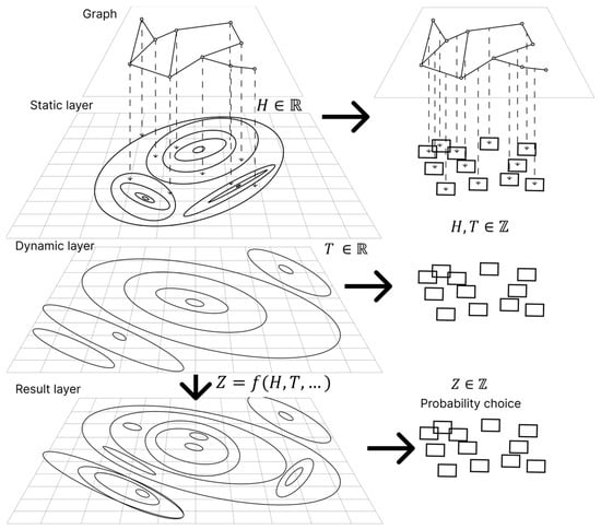
Figure 1.
Dividing information into layers in ACO.
The original ACO used the formula for the probability transition (1) from vertex i to vertex j, which used information about the arc length and pheromone [3,4].
where is the probability of transition along arc for ant agent k at iteration (the ant agent is at a certain vertex, i are arcs along which the agent can move, and is set); is the value of arc i from at iteration t. is the value of arc i from (the value inverse to the arc length is taken), is the value of the criterion for ant agent k at iteration t, and are the parameters of multiplicative convolution, is the parameter of “weight evaporation”, allowing a reduction in the influence of previously found solutions, and is the parameter of added weights (due to normalization in the probability formula, it has no effect on the operation of the algorithm, and it is recommended to set ). The probability of an arc being selected by an agent ant (1) is determined by the multiplicative combination of the arc length and the amount of pheromone, taken with weighting coefficients . The multiplicative convolution can be expressed as the resulting arc weight, . To calculate the probability taking into account the resulting weight , it is necessary to normalize to satisfy the condition for .
3.3. Modification of ACO in Matrix Formulation
For a parametric problem, the graph vertex is the admissible value of the parameter , and the arcs connect all the parameter values with neighboring numbers and for . Since arcs in such graphs do not carry information about the movement capabilities of the agent ant (the agent ant can move to any vertex of the next parameter) and the weight pheromone is left on the vertices, the arcs are fictitious and the data structure for the problem under consideration can be represented as a list of parameters, each parameter having a list of values [45]. Since the number of admissible values for each parameter is different, then to bring all parameters to matrix form, it is necessary to supplement the values of vectors to , obtaining a matrix . Setting the initial value of the layer or for the added parameter values equal to zero will ensure a zero probability of selecting these parameters, and the following conditions will be met for the added values: .
3.3.1. New Probability Formula Without Taking into Account the Heuristic Parameter
In this case, in parametric problems or other problems in which there is no a priori information about the efficiency of the agent’s movement (layer ), Formula (1) changes and only one normalized factor remains in it:
As a result, ACO stagnates at the early stages to the first rational solution found [1,45]. To solve the problem of stagnation at the early stages and improve the exploitation strategy, it is proposed to add information to the probabilistic formula related to the number of visits of agents to the graph vertices (layer ):
where is the parameter number; ; is the parameter value number ; t is the iteration number; are the coefficients of the additive convolution are the degrees of the terms of the additive convolution, which are not considered in this paper and are present in the formula due to their presence in (1). ; is the normalized weight for the value with number of the parameter with number for iteration ; is the number of ant agents that visited the vertex for the value with number of the parameter with number for iteration ; is the maximum possible number of ant agents that visited the vertices for the parameter with number .
The disadvantages of linear convolution and the mutual compensation of terms are an advantage for a probabilistic formula [45]. According to the results of mutual compensation at different iterations of the algorithm, different terms have a greater effect on the probability of choosing a parameter value, which allows the algorithm to maintain efficiency during operation. The first term depends only on the normalized number of weights for the parameter with number and its value with number . The second term depends on the number of visits of the parameter value by the agent, i.e., how many times the parameter value was considered in decisions. This term allows us to increase the probability of choosing the parameter values with the least number of visits. Adding this parameter makes it possible to avoid stagnation of the algorithm at the initial stage of operation. After several iterations of the algorithm, the influence of this parameter decreases due to the increased value of . The third term, on the contrary, increases when the number of solutions with a certain value of the parameter approaches the maximum number . The value of for a discrete problem can be calculated exactly by the formula The value of is static and does not change between iterations of the algorithm and can be calculated before starting work. This term helps to find the last solutions and has virtually no effect on the operation of the algorithm at early iterations.
3.3.2. Matrix Formalization of the Method
Due to the representation of all values for Formula (3) in the form of matrices, it is possible to calculate the probability matrix :
The presented matrix transformations consist of multiplying the matrix by a number, adding the matrix elements, and calculating the matrix–vector ratios, which can be easily performed on matrix calculators. It is worth noting separately the need to normalize the values of the matrix for using them in the following additive convolution: . The selection of the values of the parameters that form the solution, vector , is carried out on the basis of the probability distribution of the selection of vertices for each column of matrix using the inverse function method. For the inverse function method to work, it is necessary to calculate the matrix of distribution functions and .
At each iteration of ACO, the generation of ant agents of dimension finds solutions and calculates vector . After all ant agents from one generation have received decisions, a new state of all matrices is determined. During the movement of individual ants from one generation, matrices and do not change, which allows us to consider the movement of all ant agents as matrix transformations. To calculate the path of each ant agent, which determines the selected vertex values for each parameter, a matrix of the implementation of random variables uniformly distributed in the interval (0; 1) is generated, where is the parameter of ACO, which determines the number of ant agents (generation) at the iteration. Next, the index of the inverse function is determined for the corresponding generated number so that the following inequality is satisfied: . In this way, the index of the selected value is determined. The matrix of solutions, the paths of ant agents in the parametric graph , is determined from matrix V: . For each solution found, the value of the objective function is calculated, forming vector .
The values of matrix are updated according to Formula (1), defined in matrix form: . The discrepancy between the dimensions of and is resolved by adding the value of the element of vector only for the vertices, the values of the parameters that the ant agent selected, defined by matrix . The algorithmic record of this procedure can be represented as , with cycles over the variables and .
3.3.3. Modifications of the Method for the Parametric Optimization of a System with Negative Values of the Objective Function
In the probability Formulas (2)–(4), as in the original Formula (1), the negative value of the pheromone weights leads to errors in the probability formula and failures in the operation of ACO, i.e., Provided that ( determines the set of parameter values for which a negative value of the objective function is obtained), it is necessary to ensure the transformation .
The simplest transformation will be a shift in the value of the objective function by the largest value in absolute value. . The difficulty of the transformation in Formula (5) lies in the need to calculate the shift before the method can work.
Another option for the transformation is to use the absolute value of the objective function. . The transformation requires changing the direction of optimization and using it only for positive or negative objective functions.
In this case, Formulas (3) and (4) use the normalized value , which can be calculated as , which does not impose restrictions on the values of and can be used when .
3.4. Modification of the Ant Method Using a Hash Table
The use of modifications of ACO for parametric problems of optimizing model hyperparameters assumes high time costs for calculating the values of the objective function in an analytical or simulation model compared to the running time of the modified ACO. In the case of executing ACO on an SIMD computer, the acceleration of the algorithm obtained as a result of matrix formalization will be offset by the long time required to calculate the objective function in the model.
In the case when performing calculations on the model is possible only in sequential mode, parallel operation of ACO is not required. The proposed modifications are capable of working with a model in which asynchronous access to a model operating in parallel mode is possible. In such a case, it is usually assumed that the model is launched on a cluster or supercomputer. Another method that can be used together with parallelization of model calculations is intermediate storage of the results of calculating the objective function. This paper proposes to use a hash table as temporary storage, implementing matrix transformations of the ant agent path matrix into a vector of hash functions , with subsequent checking of the path in the hash table. If , then or else . The presented actions change the behavior of the algorithm as a result of checking the condition, which makes it impossible to perform these actions on an SIMD accelerator, but parallel execution on an MIMD computer is possible, parallelizing into threads.
With this approach, it is possible to consider various modifications of ACO that perform different actions when finding a value in a hash table. The point is that if the value is found, then there is an ant agent that has passed along this path in previous iterations, and a change in the behavior of the new agent will lead to the possibility of all agents not converging on one solution at the iteration but continuing to search for new, not yet considered solutions. As a result, ACO will feed new, not yet considered solutions to the computing cluster, ensuring a uniform load on the cluster. With such a formulation of the problem, the proposed modifications of ACO allow solving problems of reordering parameter sets, when sets of parameter values are sequentially sent to the computing cluster, and ACO determines the order of sending.
The following modifications of ACO are proposed in this paper [45]:
- ACOCN (ACO Cluster New): This is classic ACO that uses a hash table and obtains the values of the objective function without accessing the computing cluster. If , then .
- ACOCNI (ACO Cluster New Ignor): If the ant agent has found the already-considered solution, then this ant agent does not change the state of the dynamic layers described by matrices and , i.e., it is ignored. If , then .
- ACOCCyN (ACO Cluster Cycle N): If the ant agent has found the already-considered solution, then it performs a further cyclic search for a new solution. The cycle is limited to iterations; if a new solution is not found, then the solution is ignored.
- ACOCCyI (ACO Cluster Cycle Infinity): If the agent ant has found a solution that has already been considered, then it performs a further cyclic search until a new solution is found.
The ACOCCyI modification differs from ACOCNI in that the ACOCCyI modification guarantees that agent ant paths are found in one iteration, while in the ACOCNI and ACOCCyN modifications, .
3.5. Matrix Modification of the Ant Colony Method for Running on SIMD
The algorithm for the matrix modification of ACO using hash tables when running on SIMD computers, using computers on the CUDA platform as an example, consists of three stages (Figure 2):
- Calculation of matrix : The following are performed sequentially: the calculation of or , to obtain the values of the normalized matrix or , respectively; calculation of matrix and then vector ; and calculation of the transition probability matrix and the distribution function matrix . Since at the first stage all matrices have the dimension and vectors have the dimension , then all actions of the algorithm are performed in parallel on threads, where each thread performs operations for one parameter. When optimizing the algorithm, one can refuse to calculate matrix and calculate vector simultaneously with matrix .
- Calculation of the ant agent decisions and : The following are performed sequentially: the generation of matrix and calculation of position ; and the determination of and the calculation of vectors and , necessary for working with the hash table. One of the modifications of ACOCN, ACOCNI, ACOCCyN, and ACOCCyI is performed, based on the results on which vector is determined. This stage can be performed in threads on SIMD and MIMD computers. In this case, the operations necessary for calculating matrix , within each thread can be performed on additional threads for each thread of the ant agent.
- Calculation of the new values of matrices and : First, all values of matrix are reduced—evaporation ,—and then, the values from ant agents are added: . The values of matrix are changed in a similar way: . This algorithm can be executed on parallel threads, each of which calculates the values of a separate parameter.
The algorithm repeats a specified number of iterations, which determine the criterion for stopping the algorithm.
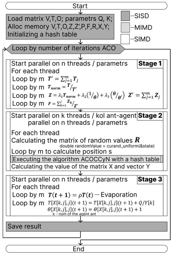
Figure 2.
Algorithm for matrix implementation of ACO on SISD, SIMD, and MIMD components.
Figure 2.
Algorithm for matrix implementation of ACO on SISD, SIMD, and MIMD components.

In some cases, it may be appropriate to combine stages to reduce the number of transitions from the GPU to the CPU when using CUDA technology. It is possible to combine the third and first stages in order to perform a sequential change in the states of matrices and and calculate matrix on threads. This algorithm requires the creation of an initial matrix and vector .
It is also worth highlighting the implementation using CUDA technology, in which the number of threads and the number of blocks can be specified. In such an algorithm, all three stages are performed in parallel on blocks, where each block defines a separate behavior of the ant agent, and the update of matrices and and the calculation of matrix are performed in parallel on n threads. With this formulation, only one call to the method implemented on a GPU with CUDA technology is required.
3.6. Graph Structure for Parametric Optimization
Separately, it is worth noting the acceleration of the algorithm due to division into threads, where determines the number of parameters in the problem. At the same time, many benchmarks and parametric problems have a small number of parameters, , usually equal to two, for which parallel calculations are ineffective. For numerical parameter values obtained by discretizing continuous parameters with a certain accuracy, the number of such values for one parameter m can be very large. This paper considers an algorithm that allows the division of a set of parameter values into separate sets, forming related successive layers of values related to one parameter. The ant agent selects not one vertex of the parameter value but several values from the vertices of the set, calculating the final value of the parameter by linear convolution of the obtained values in all layers.
For example, when considering a two-criterion benchmark with with an accuracy of , the following layer configurations can be considered:
- Standard: The standard configuration for and uses 201 vertices. See Graph A in Figure 3.
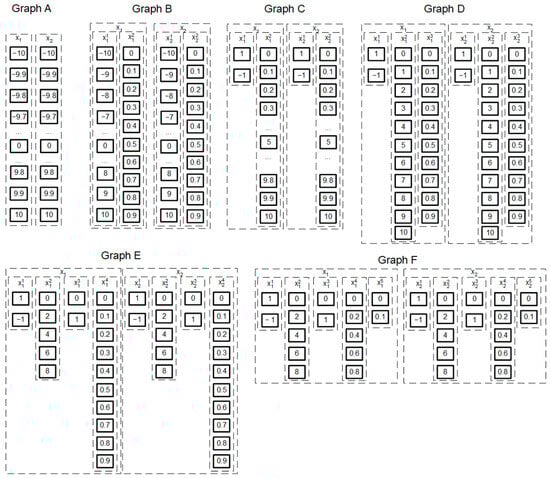 Figure 3. Decomposition of parameter values into layers.
 - Separation of the real part: Each layer is divided into the integer part in the interval [–10, 10] with a step of 1 (21 vertices) and the fractional part in the interval [0, 0.9] with a step of 0.1 (10 vertices). . In total, there will be 2 layers for each parameter in the parametric graph. The total number of solutions will increase to 44,100 due to the appearance of several zeros. See Graph B in Figure 3.
- Selection of the negative part: Each layer is divided into the sign (2 vertices) and the positive part in the interval [–10…10] with a step of 0.1 (101 vertices). . In total, the parametric graph has 2 layers for each parameter and 40,804 vertices. See Graph C in Figure 3.
- Separation of integer, real, and signed parts: Each layer is divided into the sign (2 vertices), the integer part in the interval [0, 10] with a step of 1 (11 vertices), and the fractional in the interval [0, 0.9] with a step of 0.1 (10 vertices). . In total, the parametric graph will have 3 layers for each parameter and 48,400 solutions. There are 7999 more solutions here than in the standard graph, since there are “extra” solutions, for example, . See Graph D in Figure 3. This graph is intuitive. When increasing the precision of parameter discretization, for example, to 0.01, it is necessary to simply add the corresponding layers for each parameter in the interval [0…0.09] with a step of 0.01 (10 vertices).
- In addition to selecting the integer, real, and sign parts, it is possible to decompose layers in the intervals [0, 10]. As a result, the parametric graph will have 4 layers for each parameter. ; is a sign layer (2 vertices), and corresponds to one vertex, , from Graph D: comprise even numbers from the interval [0, 8], and takes 2 values, 0 or 1. This graph is designated in Figure 3 as Graph E.
- Further decomposition of not only the integer but also up to 5 layers for each parameter of the real part. . See Graph F in Figure 3.
To decompose numerical values of parameters into separate layers, an automatic decomposition system is proposed, based on decomposing the range of values into simple factors to determine the minimum number of values for each layer . The number 10 is decomposed into two simple factors, 2 and 5, that is, into 2 layers with 2 and 5 vertices, respectively (Graph E, Figure 3). If the values change in the interval [0, 10] (11 vertices), then it will not be possible to divide this layer. But for values in the interval [0, 11] (12 vertices), it is possible to distinguish 3 layers with 2, 2, and 3 vertices. To determine the values at the vertices, one can use the formula , where is the parameter number; is the layer number for this parameter; and is the vertex number in the layer. Since the most appropriate and logical division is into integers, tenths, and hundredths, each such layer consists of 10 vertices, which can be decomposed into 2 more layers. As a result, with such a decomposition, many layers are obtained for each parameter with a maximum number of values in one layer, , which significantly reduces the number of calculations and makes the operation of the multithreaded system efficient.
4. Results
4.1. Analysis of the Efficiency of Application of the Proposed Modifications of ACO
Analyses of a new probabilistic formula, the interaction of ACO with a hash table, and the modifications of ACOCN, ACOCNI, ACOCCyN, and ACOCCyI were carried out on software developed in Python 3.12 (https://github.com/kalengul/ACO_Cluster (accessed on 9 April 2025); the entry point is the main.py file, and the task and parameters of the ant colony method are specified through the setting.ini files). This software explores a single-threaded version of ACO for the convenience of testing and research of the proposed modifications. In addition, the software has the ability to run in multi-process mode (taking into account the presence of Global Interpreter Lock—GIL) and interact with the model through a socket connection to calculate the values of the objective functions. The absence of multithreading allows us to consider the effectiveness of the method modifications in the worst case.
During this study, estimates of the mathematical expectation of the algorithm’s running time, estimates of the probability of finding an optimal solution (if the value of the objective function is known), and estimates of the mathematical expectation of the iteration number at which the optimal solution was found were calculated. Testing was carried out on various benchmarks and large-scale test graphs [46,47].
Figure 4 shows the graphs of the “multi-function” function (a) and the “Schwefel” function (c), and Graphs (b) and (d) show the estimate (based on the results of 3000 runs in the direction of minimizing the values of the objective function) of the mathematical expectation of the ordinal number of the solution, in which the given values of the parameters and were considered. The estimate of the mathematical expectation of the iteration number resembles the outlines of the function graph. As a result, statistically optimal sets of parameter values were determined at early iterations. After finding the first optimal solution in early iterations, the ACOCCyI algorithm did not stop working despite the convergence of the algorithm and still allowed the determination of all optimal solutions.
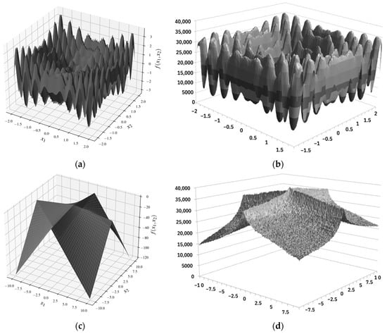
Figure 4.
Graphs of the “multi-function” function (a) and the “Scheffel” function (c). Graphs (b) and (d) show an estimate of the mathematical expectation of the ordinal number of the solution on which these values of the parameters were considered.
4.1.1. Investigation of a New Probability Formula and the Influence of Additional Terms
Figure 5 presents an analysis of the efficiency of applying the new probability formula, Formula (3). The influence of using different terms of the additive convolution on the estimate of the probability of finding the optimal solution for a given number of iterations (Figure 5a) and the estimate of the mathematical expectation of the iteration number at which the first optimal solution was found (Figure 5b) are studied. Testing was carried out on the benchmark “Carrom table function”:
with discretization up to (201 values of each of the parameters and ) with 25 agents per iteration (). Since ant agents perform probabilistic, stochastic route selection, estimates of the mathematical expectation were calculated as a result of 200 launches of ACO with a limited number of iterations. The dashed lines indicate confidence intervals of estimates at a significance level of 0.95. The original ant colony method has no additional terms: , , and (shown in the figures by the red lines). The results of the research revealed that the presence of the second term allows for the determination of the optimal solution at the earliest iterations, and its absence leads to stagnation of the algorithm. At the same time, the third term does not have a special effect on the efficiency of ACO in the process of searching for the optimal solution and works only when solving the problem of rearranging parameter values for sending to the computing cluster.
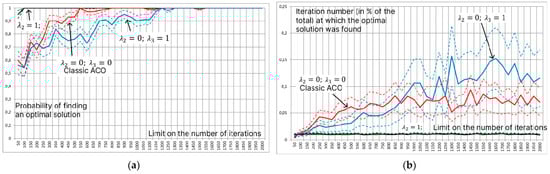
Figure 5.
Estimation of the probability of finding an optimal solution for a given number of iterations (a) and estimation of the mathematical expectation of the iteration number at which the first optimal solution was found (b) under various restrictions on the number of iterations. The dotted lines indicate confidence intervals of estimates at a significance level of 0.95; the color of the dotted line corresponds to the color of the estimate.
4.1.2. Analysis of Parametric Graph Decomposition
When studying the possibility of decomposing all parameter values into separate layers with subsequent linear convolution, it was found that ACO works well with low-dimensional graphs. Figure 6 shows graphs of the estimated probability of finding an optimal solution for a given number of iterations (Figure 6a) and the estimated mathematical expectation of the iteration number at which the first optimal solution was found (Figure 6b) for the structures shown in Figure 3 (). The red graph represents a graph similar to the graphs applicable in ACO-LSTM, in which each parameter forms a layer. The graphs show that the maximum decomposition to Graphs E and F not only allows us to find the optimal solution earlier but also determines it with a higher probability even at a small number of iterations. Graphs B and D also demonstrated high efficiency, in which the decomposition of a real value is carried out into tens, integers, tenths, hundredths, etc. The automatic creation of such graphs is significantly simpler than the creation of Graphs E and F.
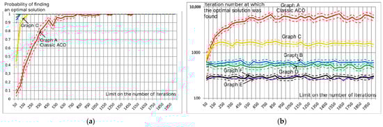
Figure 6.
Estimation of the probability of finding the optimal solution for a given number of iterations (a) and estimation of the mathematical expectation of the iteration number at which the first optimal solution was found (b) for the structures shown in Figure 3.
4.1.3. Analysis of Modifications of the Ant Colony Method Using a Hash Table
An analysis of the efficiency of modifications of the ant colony method associated with working with a hash table was carried out for problems of small and large dimensions [45]. The problem of small dimension is represented by the benchmark “Carrom table function” with discretization up to 10−2; for large dimension, a practical problem consisting of 13 parameters was considered, totaling more than 109 solutions. The proposed modifications ACOCN, ACOCNI, ACOCCyN, and ACOCCyI were compared with classic discrete parametric optimization close to solving the QAP, and they were used without using a hash table, i.e., if the ant agent goes along an already-explored path, the pheromone will be added. The objective of this analysis is to determine the optimal modifications of ACO for the purpose of further comparison of the best modification with other metaheuristic algorithms.
In the problem of small dimensions, the optimal values of the system parameters are already determined at early iterations, and the use of the modifications ACOCN, ACOCNI, ACOCCyN, and ACOCCyI is distinguishable only when continuing the search in order to ensure the enumeration of all parameter values or the search for all optimal solutions. In the case of the problem of large (more than solutions in total) dimensions, the ACOCN and ACOCNI algorithms are close to stagnation and begin to converge to good, rational solutions. The ACOCCyN and ACOCCyI algorithms allow one to completely avoid stagnation processes due to a repeated cyclic search for solutions and demonstrate high efficiency (Figure 7). . The dotted lines in the figure indicate confidence intervals for a significance level of 0.95. Already with 50 ant agents per iteration, the ACOCCyN and ACOCCyI algorithms, with a probability of more than 90%, determine the optimal solution in iterations. A further increase in the number of ant agents per iteration leads to an increase in the iteration number at which the optimal solution will be found.

Figure 7.
Estimate of the probability of finding the optimal solution for 105 iterations (a) and estimate of the mathematical expectation of the iteration number at which the first optimal solution was found (b) depending on the number of ant agents at the iteration. Estimates for modifications are ACOCN, ACOCCyN, and ACOCCyI.
The main disadvantage of the ACOCCyN and ACOCCyI modifications is the need to perform additional iterations. This procedure requires additional time, which increases the average time of the path search by one agent ant (Table 1). However, additional iterations do not have a significant effect, increasing the path search time by no more than 20% (the ACOCCyN modifications find the optimal solution on average two times faster).

Table 1.
Estimation of expected value of time of solution search by one agent (in seconds).
4.1.4. Comparison of Proposed Modifications of ACO with Genetic Algorithm (GA), Particle Swarm Optimization (PSO), and Simulated Annealing (SA)
To evaluate the efficiency of the proposed modifications of the ant colony method, we compare them with the genetic algorithm, particle swarm method, and simulated annealing. This analysis was conducted on five two-criterion benchmarks , with a limit of of the considered solutions. The estimate of the mathematical expectation and confidence intervals of the found optimal values of the function was determined based on the results of 500 runs.
Since the ACO, GA, and PSO algorithms specify the population size as , the number of algorithm iterations is determined as . For the SA algorithm, a multi-start approach was used, where the number of starts was set to be equal to the population size, K. The parameters of the studied algorithms (implementation of GA, PSO, and SA—https://github.com/kalengul/ACO_Cluster/tree/master/GA%2C%20PSO%2CSA, accessed on 9 April 2025) are as follows:
- ACOCCyI—. With the use of elitism, the number of elite ant agents is two times greater than the number of agents per iteration. Since the modifications under consideration require the discretization of parameters, the values of and were determined with an accuracy of , presented as Graph F with a total number of possible solutions of 1.96 × ;
- GA—An algorithm with Linear Crossover is used, in which Random Alpha is additionally determined; Rank Selection is carried out for a group of individuals, and Random Selection is carried out for each individual from the selected group, mutation with adaptive change, and the use of elitism. .
- PSO—.
- SA—.
For this analysis, the number of individuals per iteration varied from 50 to 500. Figure 8 shows the results for the benchmarks: the root function (a) and the “Bird” function (b). Table A2 in Appendix A describes all the values of the estimates of the mathematical expectation of the deviation of the found value from the optimal one, indicating the confidence intervals for a significance level of 0.95.
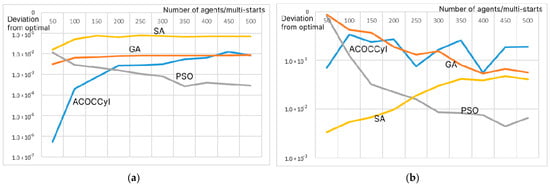
Figure 8.
Estimation of the mathematical expectation of the deviation of the optimal value found by the algorithm from the optimal value of the root function (a) and the “Bird” function (b) depending on the number of agents/multi-start for 105 iterations.
When analyzing the results in Figure 8 and Table A2 in Appendix A, we can conclude that the proposed ACO modifications work well for a small number of agents per iteration. For 50 agents per iteration, ACO did not show the best results only on the complex “Bird” benchmark , for which the SA and PSO algorithms turned out to be the best. At the same time, the ACO modifications did not use additional heuristic information. Moreover, among all the algorithms and all the values of the number of agents at the iteration, ACO determined the best value of the root function . For the remaining functions, the PSO method showed the best values. The results obtained both for the GA, PSO, and SA algorithms, and for the proposed modification of ACO with additive convolution and the use of a hash table, correspond to the results demonstrated in the following works: [34,36,39,40,41].
4.2. Analysis of the Parallel Method of Ant Colonies
Based on the research results, the probabilistic Formula (3) is implemented for the efficient operation of the parallel ACO without taking into account the third term for large-scale problems while taking into account the third term for small-scale problems. The absence of the third term will reduce the number of operations for calculating the formula and will eliminate the need to calculate and store matrix . Algorithms using a hash table are studied: ACOCNI and ACOCCyN with a limit of 100 additional iterations. The parametric problem is necessarily decomposed into layers up to Graph F, with a maximum number of vertices in one layer equal to five. This decomposition is required to increase the number of layers, each of which can be processed in a separate thread on an SIMD computer and to reduce the number of additional vertices required to represent Graph F as a matrix .
To study the efficiency of the parallel ACO, software was developed in C/C++ for operation on CUDA graphics cores for GPUs manufactured by NVIDIA https://github.com/kalengul/ACO_SIMD, accessed on 9 April 2025 (the entry point is the kernel.cu file, the parameters of the algorithm and the research procedure are specified in the parametrs.h file, and the result is output to the log file). Also, a matrix formalization of the ACO modification was implemented to perform calculations on the CPU. Modern processors have sets of extensions for executing matrix instructions for parallel data processing, for example, SSE (Streaming SIMD Extensions), AVX (Advanced Vector Extensions), and others. The comparison was carried out with the classic implementation of ACO (implemented as separate functions in the same software), built in C++20 using objects and optimized for efficient solutions of the same problems as matrix modifications.
It is worth noting the features of the random number generator assignment when performing calculations on CUDA. CUDA technology involves the use of independent blocks and threads with minimization of communication over shared memory. Unlike matrix processors’ CPU, for which one random number generator with a random seed value at each iteration or run is sufficient, CUDA requires setting a unique initial seed value for each thread. In the case of a match in the sequence of pseudo-random numbers, the ant agents will make the same probabilistic choice and receive the same paths. As a result, the number of solution matches in the hash table increases sharply and the operating time of the ACOCCyN modification increases sharply. To solve this problem, information about the block number (blockIdx.x), thread number (threadIdx.x), and time (clock64()) was used when calculating the seed.
The studies of acceleration of the running time of matrix modifications of ACO were carried out on the benchmark “Schaffer function”:
with an accuracy of for different numbers of parameters and solving the minimization problem. . When decomposing one parameter, 21 layers are implemented. In this case, problems with 2 (classic benchmark), 4, 8, 16, 32, and 64 parameters were considered. In practice, two-criterion problems of small dimensions are rare, and simpler algorithms are used to solve them. As a result of the development of computing systems, matrix computers, and parallel instruction processing technologies, large-scale problems are of increasing interest; for example, for a problem with 64 parameters, the number of layers reaches 1344. The optimization of ultra-large-scale problems is relevant and feasible but requires further research [48]. The proposed matrix modification depends on the computing power: the number of cores, the maximum possible number of SIMD threads, or the number of blocks and threads in one block when calculating using CUDA technology.
Time interval measurements were performed on an NVIDIA GeForce GTX 3060 Ti Notebook video card and an Intel Core i5-12450H processor which has 16 Gb of Random Access Memory. The mathematical expectation of the execution time of the algorithm and its individual stages was estimated when comparing the classic ACO, the matrix implementation on the CPU, and the implementation on the GPU with CUDA technology in three variants: stages 1 (obtaining matrix ), 2 (searching for solutions of ant agents using a hash table), and 3 (changing the states of matrices and ) separately; stages 1 and 3 combined; and all stages executed in one algorithm. The results of calculating the time for the ACOCCyN algorithm and confidence intervals for a confidence probability of 0.95 obtained for 100 runs are presented in Table 2. Table A1 in Appendix A contains detailed measurements of various modifications of the algorithms on different problem dimensions, broken down into individual stages. According to the research results, the matrix representation of ACO provides an acceleration of 5–6 times when using CUDA technology and 12 times when executing the algorithm on the CPU. It is worth noting separately that doubling the dimension doubles the execution time of the matrix implementation on the CPU and the classic algorithm.
Table 2.
Estimation of the mathematical expectation of the execution time (in ms) of 500 iterations by 500 agents when searching for the optimum of the Schaffer function on graphs of different dimensions using different algorithms.
The standard, classic ACO method does not interact with the hash table in any way, stagnating at good solutions but not violating the sequence of SIMD calculations. The analysis of the running times of ACO modifications using a hash table and without it showed that for classic ACO and matrix ACO, the hash table does not cause significant delays since the ant agents in these algorithms determine a unique set of values at each iteration and since interaction with the hash table is reduced to checking the existence of a solution and adding a new value (Table 3). The implementation of matrix ACO based on CUDA requires the synchronization of threads when interacting with the hash table, which increases the time for this modification by more than four times.
Table 3.
Speeding up the algorithm without using a hash table of 500 iterations by 500 agents when searching for the optimum of the Schaffer function on graphs of different dimensions using different algorithms.
Figure 9 shows the ratio of the second stage (calculation of matrices and ; calculation of vectors , and ; and operation of modifications ACOCN, ACOCNI, ACOCCyN, and ACOCCyI) of the algorithm operation to the total operating time of the algorithms with (a) and without (b) a hash table. For algorithms without a hash table, the second stage only determines the path of the ant agent and calculates the objective function, the parallel calculation of which is performed quite quickly. As the problem dimension increases, the share of time in calculating the agent paths also increases. The presence of a hash table, even taking into account only the check for the absence of a record and the addition of a new one, significantly increases the operating time of the second stage. As a result of the conducted research, it can be concluded that for algorithms operating without a data warehouse, it is necessary to optimize the work with the T and layers, and when using a hash table, it is necessary to optimize the stage of interaction with the hash table.
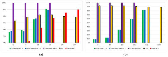
Figure 9.
Histograms of the ratio of the execution time of the second stage of the matrix algorithm to the total execution time of the algorithm for modifications with the use of a hash table (a) and without it (b).
The analysis of the effect of the matrix modification of ACO on the efficiency of the method with varying numbers of ant agents per iteration showed the relative stability of the efficiency of the methods (Figure 10). Each ant agent finds a path only at the second stage and is not involved at stages 1 and 3, and the second stage in the proposed algorithms involves searching for a path by each agent in a separate SIMD/MIMD thread. Up to 512 agents, the division into threads occurs effectively, and it is possible to increase the efficiency of the modification (in terms of execution time).
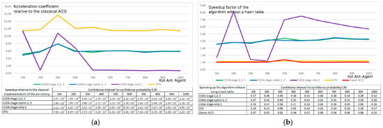
Figure 10.
Speed-up factor of matrix modifications of ACO when changing the number of ant agents per iteration for a problem with 84 layers for the ACOCCyI modification (a) and without a hash table (b).
Additionally, studies were conducted on the Intel Core i5-8300H CPU, which has 8 Gb of Random Access Memory, and NVIDIA GeForce GTX 1050 Ti GPU for a 336-layer structure. . Based on the results of 100 iterations, the greatest acceleration of 12.12 times (±0.76 confidence interval for a confidence probability of 0.95) was achieved by the “CUDA stage optim 1, 2” algorithm. The CPU provided an acceleration of 10.01 times (±0.51).
4.3. Analysis of the Optimal Structure of a Heterogeneous Computer Based on SIMD and MIMD Components
Based on the calculated estimates of the duration of the individual stages of work, it is possible to estimate the acceleration coefficient of the matrix modification for individual stages. As a result of such an assessment, it is possible to calculate the time of the following stages:
- Start of the algorithm and creation of the necessary data structures (Stage Start): Since this stage is performed in a single copy, its execution is possible only on SISD systems, and the acceleration of this stage is carried out using FPGA. When analyzing the efficiency of the system, the execution time of this stage is constant and mandatory; it can be neglected when constructing a heterogeneous computer.
- Iteration overhead (Stage Delt): This overhead is associated with counter incrementing, context switching, calculating the timing of nested stages, etc.
- The first stage (stage 1), associated with matrix transformations to obtain matrix , can be performed on SIMD computers.
- The second stage (stage 2), associated with the search for paths by ant agents, can be performed on SIMD computers in the absence of interaction with the hash table. When interacting with the hash table, the result of operations, the duration of individual transformations, and the subsequent behavior of the algorithm are undefined and depend on the results of the system’s operation. As a result, this stage is best implemented using an MIMD component or an SIMD accelerator and an MIMD component together.
- The third stage (stage 3), associated with updating matrices and , consists only of matrix transformations and can be performed on an SIMD accelerator.
The design example of the optimal structure of the heterogeneous calculator will be based on the time characteristics and acceleration factors of matrix implementation on the CPU in comparison with the classic implementation for 500 iterations and 500 ant agents when solving the problem of calculating the optimum of the Schaffer function with 336 layers in the data structure using the ACOCCyN algorithm. The estimated mathematical expectation of the execution time of the classic modification is s, the time without taking into account the SISD component is , and the proportion of the parallelized fragment is , which indicates the inefficiency of deep optimization of the SISD component. High delay is associated with the need to initialize the hash table, which can be accelerated by a multithreaded computer, so for the classic algorithm without using a hash table, . Using a hybrid computer consisting of SIMD and MIMD components allows us to reduce the time of matrix algorithm , which is divided into stages as follows: , where and are the operating time of the SIMD component for stages 1 and 3, respectively, and is the operating time of the SIMD and MIMD components at the second stage. To further divide the operating time of the SIMD and MIMD components in the second stage, the operating time of the method modification that does not use the hash table is used, since this modification can be entirely performed only on an SIMD accelerator. The times for individual stages for different modifications are given in Table A1 of Appendix A. As a result, the total execution time of the SIMD block is , and the time of the MIMD block is , without taking into account the SISD component .
To evaluate the efficiency and determine the acceleration factor, it is necessary to calculate the acceleration obtained by using the SIMD calculator. Since the Intel Core i5-12450H central processor connects the matrix accelerator for all matrix-related calculations, it is difficult to accurately estimate the acceleration factor associated with the intentional use of the SIMD accelerator on the CPU. The estimate is used. By measuring the time taken by the classic algorithm, it is possible to determine the ratio of the execution time of the MIMD fragment to the total execution time of the parallelized block . The share of the SIMD fragment will be .
If there are processors (cores) in the computer, it is possible to run several matrix modifications of ACO in parallel with different initial data as well as run them sequentially with the possibility of parallel work with the hash table in the MIMD fragment. In the first case, the total execution time of or less tasks simultaneously will be equal to . In the second case, , where is the execution time of the matrix modification taking into account the acceleration of the MIMD fragment on threads. where is the acceleration coefficient on cores. . Therefore, , and the acceleration factor on q processors associated with the use of the matrix parallel algorithm relative to the classic parallel algorithm is . In the ideal case, when we obtain (Figure 9). When , the acceleration of the MIMD fragment remains effective.
It is also possible to speed up the matrix method by increasing the number of SIMD accelerators and dividing the layers for parameters/ threads into different accelerators. With accelerators, the speed-up factor can be calculated as the ratio of the running time of the matrix modification of the algorithm to the running time of the matrix modification under the condition of acceleration of the execution process on SIMD accelerators. . In Figure 11, the additional right axis shows the change in the speed-up factor depending on the number of SIMD accelerators in the optimal case, in which . for and ; the difference from the obtained value of 12.72 (Table 2) is due to the acceleration of the SISD component, which performs the initialization of the hash table and data loading. The maximum value of the coefficient can be calculated under the condition . We obtain .
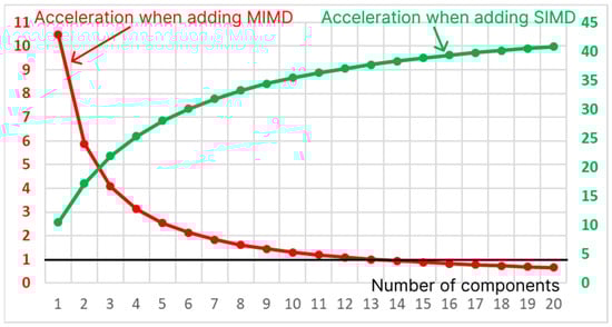
Figure 11.
Acceleration due to the increase in the number of SIMD accelerators and MIMD cores.
In general, the acceleration factor for computing using MIMD processors and SIMD accelerators can be calculated using the formula , using optimal MIMD and SIMD components, i.e., where .
4.4. Analysis of the Optimal Structure of a Heterogeneous Computer Taking into Account the Reconfiguration Mechanism
To achieve maximum acceleration, various computing structures containing different numbers of cores and accelerators are required. In practice, the number of cores and accelerators in a hybrid computing device is fixed. As a rule, due to design features, is satisfied. Starting from a certain value, , the increase in the acceleration coefficient for a given becomes insignificant. Therefore, it is advisable to form two structures in the computing device:
- A homogeneous MIMD structure of general-purpose cores without SIMD accelerators;
- A hybrid structure containing MIMD cores and SIMD accelerators, in which cores interact with one accelerator.
In this formulation, the overall acceleration coefficient is the sum of the acceleration coefficients of the homogeneous MIMD structure () and the hybrid structure . , where . To calculate the optimal number of cores in the hybrid structure, we calculate the derivative with respect to or the acceleration factor using the quotient differentiation rule for the hybrid acceleration factor.
Substituting the values for the problem studied in the previous subsection, we obtain , and . For example, in the case of one SIMD accelerator and 16 MIMD cores, it is recommended to assign 5 MIMD cores to a homogeneous MIMD structure and add 11 MIMD cores to the SIMD accelerator in a hybrid structure. In this case, If there are five SIMD accelerators in the system, then only one MIMD core can be freed from the hybrid structure .
The resulting final formulas depend on the ratios of the volumes of parallelized calculations, ; the ratio of the volumes of SIMD and MIMD components, ; the acceleration coefficient of the SIMD accelerator compared to the MIMD core, ; and the planned parallelization coefficients for MIMD and SIMD components, , respectively. Figure 12 shows the dependencies of the presented characteristics for the CPU matrix modification of ACO for different problem dimensions.

Figure 12.
Changing the coefficients (yellow line, left axis) and (red line, left axis) and (green line, right axis) depending on the problem dimension for the matrix modification of the ACO running on the CPU.
Figure 12 shows that the influence of the MIMD component decreases significantly with increasing problem dimension. The coefficients and tend to unity and, for a dimension of 336 layers, are greater than 0.9, i.e., 90% of all calculations are concentrated in the SIMD accelerator.
4.5. Analysis of the Efficiency of Matrix Modification of the Algorithm on a GPU Using CUDA Technology for the Case of Repeated Searches for Solutions by the ACOCCyN Algorithm
The above example of calculating the efficiency of the implementation of the matrix method of ant colonies on the CPU provides maximum acceleration of the algorithm due to the fact that all ant agents find unique paths and interaction with the hash table. It is limited only to determining the absence of a route and entering a new record. In this form, there will be no differences in the operation of the ACOCN, ACOCNI, ACOCCyN, and ACOCCyI algorithms.
At the same time, on the GPU, due to the difficulties with generating random numbers, the same paths are repeatedly found, which greatly reduces the efficiency of the algorithm due to the need to conduct a repeated search by the ACOCCyN algorithm. But the obtained time characteristics allow us to estimate the acceleration coefficients for the ACOCCyN algorithm, in which the influence of the MIMD component is more significant.
To perform the matrix implementation on the GPU using the ACOCCyN algorithm for a problem with a dimension of 336 layers, an average of 3220.7 additional iterations were required (estimated by 100 runs). The value of is 2.7 times longer than the CPU execution time. At the same time, and . The time of the MIMD component is significantly increased, since various options for searching for a value in the hash table are possible, either by adding a new value to it or re-searching for the path. As a result, the acceleration factor and the coefficients and remained unchanged, since they depend only on the classic implementation of ACO. As a result, the acceleration factor for 1 SIMD accelerator and 16 MIMD cores of the computer (11 cores for the hybrid structure) is , and that for 5 SIMD accelerators (15 cores of the hybrid structure) is . Such an increase in the efficiency of the algorithm compared to the algorithm on the CPU is due to a significant acceleration of the SIMD component of the GPU. For and , . Theoretically, the acceleration of the SIMD component allows for the acceleration of the classic ACO by 22 times.
4.6. Application of Modifications of ACO in Searching for Optimal Values of the SARIMA Model Parameters
The proposed and studied modifications of ACO were applied to solve the practical problem of calculating the values of the parameters of the SARIMA model for forecasting the volumes of passenger and cargo transportation by airlines of the Russian Federation. Before the 2020 restrictions associated with the COVID-19 pandemic, the volumes of passenger and cargo transportation by air had a clear oscillatory component with a fixed small trend (up to 5% per year) and a weak noise component (up to 10%). The stability of such a series made it possible to quite accurately predict the values of the indicators for the next year. In this case, the following indicators of the air transport industry were analyzed: passenger flow; completed passenger turnover; seat occupancy rate; average number of hours per flight; distance per flight; completed tonne-kilometers; and the amount of transported cargo and mail and others on both domestic and international flights, divided into regular and irregular. There were more than 30 indicators in total. After the 2020 lockdown, the volumes of indicators related to passenger transportation dropped to 0 and showed a rapid recovery for domestic flights, having an unstable nature with a difficult-to-predict structure. To make a forecast, LSTM neural networks and SARIMA class models were considered. Due to the small sample (54 values), the use of the LSTM model showed less efficiency than the use of the SARIMA model. At the same time, for the SARIMA model, the parameter values were determined by modifications of ACO when optimizing the MAE and RMSE criteria (both a single-criterion problem for each criterion separately and a multi-criteria problem were solved). ACO has proven its effectiveness in determining better values of indicators than classic methods, such as pmdarima.arima.auto_arima, and the matrix implementation allows us not to lose too much time in searching for optimal values.
For the LSTM model, a comparison of the proposed modifications of the ACO algorithm was carried out; the ACO modification in which the heuristic information about the effective parameters of the LSTM model set the initial values of the weights and the ACO-LSTM modification. The mathematical expectation of the found solution was studied for 100 runs of the model with the following parameters: , and 50 elite ant agents. The confidence interval is specified for a confidence probability of 0.95. As a result, the ACO modification proposed in this article loses to ACO-LSTM by 1.23 (±0.12) times, and ACO with the initial values of the weights loses to ACO-LSTM by 1.08 (±0.03) times. At the same time, the modification proposed in this work allows one to rebuild the optimization of the hyperparameters of the SARIMA model without adding new information; only the data structure changes. The loss of the proposed modification of ACO compared to ACO-LSTM, in which the heuristic value of choosing the parameters SARIMA is determined based on the results of the analysis of corellograms, is 1.18 (±0.04) times.
5. Discussion
This paper has proposed a matrix formalization of ACO aimed at solving parametric problems. Based on the results of matrix formalization, it was possible to perform calculations using matrix processors and SIMD calculators. The problem statement was defined, and the data structure created from a parametric graph was considered, a graph in which each node determines a specific parameter value. For the matrix formalization of the problem, this graph was presented as a matrix; for its creation, we proposed to add imaginary vertices, the selection of which is impossible for ant agents. To solve the problem of stagnation of ACO without a priori information about the system, a new probabilistic formula for selecting a parameter value was proposed, based on the additive convolution of the number of pheromone weights and the number of visits to the vertex. At the same time, the presentation of information in ACO in the form of separate layers allowed us to not only formalize the modification of the method for solving multi-criteria problems in which additional layers are added but also determine the matrices required for the operation of the method.
ACO can be implemented as parallel computations, since the interaction of ant agents is carried out only when the state of the matrix changes. Nevertheless, the high speed of determining the solution should be correlated with the high speed of calculating the objective function for this solution, which can be difficult for parametric problems due to the use of complex analytical and simulation models. If the time spent calculating the value of the objective function is greater than the time spent searching for a set of values, then the sequential ACO will be as effective as its parallel implementation. The efficiency of ACO can be increased by storing the obtained values of the objective function and, in the case of repeating the path of the ant agent, determining the result from the storage. With such storage, this paper has proposed to use a hash table with various modifications of the behavior of ant agents that have already found the solution considered. To study the proposed changes to ACO, software was developed in the Python programming language.
In parallel calculations, it is possible to separate the matrix modification of ACO into SIMD and MIMD components and perform calculations on the corresponding equipment. To study the matrix modification of ACO, software was developed in C/C++, which implements the matrix method both on SIMD CPU accelerators and uses CUDA technology on GPUs.
6. Conclusions
According to the results of the research, when solving the problem of optimizing benchmark functions of different dimensions, it is possible to ensure the acceleration of the method by more than 12 times. The obtained results correspond to the publications on the modification of the parallel ACO for solving the TSP and QAP, in which an acceleration of up to 24 times was obtained on some problems.
Nevertheless, a 12-fold acceleration was achieved on the matrix SIMD CPU accelerator without modifying the algorithm to the specific processor architecture. When performing calculations on the GPU, only a six-fold acceleration was achieved. This is due to the peculiarities of the implementation of the pseudo-random number stream, which, with identical sequences, leads to a situation where all ant agents select the same parameter values, which, when using the ACOCCyN algorithm, leads to a repeated cyclic search.
The results of this study revealed the ratio of the volumes of code executed on the SISD, SIMD, and MIMD components of a heterogeneous computer. The share of SIMD is less than 10% of the total volume of calculations. As a result, the efficiency of using FPGA technology is possible only for initializing the hash table, which, in the case of matrix formalization, can be performed on an SIMD accelerator. The share of the MIMD component in this case is about 2%, which is due to the lack of overlap of the routes of the ant agents. For complex problems with a pronounced extremum, this estimate can change due to the operation of the ACOCCyN algorithm, the use of which is possible only on an MIMD computer. To assess the possibilities of accelerating the algorithm by using a reconfigurable heterogeneous computer containing several SIMD accelerators and several MIMD accelerators, mathematical dependencies of the acceleration factors on the algorithm parameters and the number of components were determined. Based on the results of the research, a conclusion was made about the efficiency of increasing the number of SIMD accelerators, with the acceleration factor reaching the limit of 48.176 times. When using a reconfigurable calculator, which has several components of both SIMD and MIMD and which can work both together with the SIMD accelerator and separately, the optimal division of MIMD components was determined. Based on the results, when increasing the number of SIMD components from 1 to 5, we proposed to use 11 and 15 (out of 16) MIMD components in conjunction with SIMD components, respectively, which will provide accelerations of 39 and 110 times.
Further research involves the development of the SIMD concept of the ant colony method to increase the acceleration of iterations for solving the parametric optimization problem. The design and development of algorithmic support allows for the running of the proposed modifications on supercomputers and heterogeneous computers, together with a system of computational models. Separately, it is necessary to delve into the study of the use of matrix cores and accelerators on CPUs and division of the method into SIMD and MIMD stages to improve the efficiency of their operation. It is assumed that the method will be used to solve the problem of optimizing the hyperparameters of the CALS system in the field of civil aviation. Another important development is the transition from discrete to continuous optimization by the ACO method using Gaussian distribution.
Author Contributions
Conceptualization, V.S. and Y.T.; methodology, V.S.; software, Y.T.; validation, V.S. and Y.T.; formal analysis, V.S.; investigation, V.S.; resources, Y.T.; data curation, Y.T.; writing—original draft preparation, Y.T.; writing—review and editing, V.S.; visualization, Y.T.; supervision, Y.T.; project administration, V.S.; funding acquisition, V.S. All authors have read and agreed to the published version of the manuscript.
Funding
This research received no external funding.
Data Availability Statement
The data that support the findings of this study are openly available on GitHub at https://github.com/kalengul/ACO_SIMD (accessed on 9 April 2025).
Conflicts of Interest
The authors declare no conflicts of interest.
Appendix A
Table A1.
Estimates of the mathematical expectations obtained from 100 calculations of the Schaffer function at 500 iterations by 500 agents of the ACOCCyN matrix modification.
Table A1.
Estimates of the mathematical expectations obtained from 100 calculations of the Schaffer function at 500 iterations by 500 agents of the ACOCCyN matrix modification.
| Total Number of Layers/Threads n | |||||||
|---|---|---|---|---|---|---|---|
| 42.00 | 84.00 | 168.00 | 336.00 | 672.00 | 1344.00 | ||
| Time CUDA stage 1, 2, 3 | Stage 3 | 398.46 | 409.29 | 419.56 | 440.14 | ||
| Stage 2 | 1580.51 | 1801.93 | 3275.77 | 10,297.52 | |||
| Stage 1 | 24.22 | 26.52 | 25.28 | 30.20 | |||
| Loop While | 13.09 | 17.80 | 12.25 | 23.79 | |||
| Load Data | 7.63 | 8.09 | 8.35 | 10.13 | |||
| Total Time | 2023.91 | 2263.64 | 3741.21 | 10,801.78 | |||
| Min | 0.00123 | 0.001247 | 0.011536 | 0.054558 | |||
| Max | 0.99983 | 0.995116 | 0.983309 | 0.944857 | |||
| Hash Iter. | 14,009.00 | 12,243.70 | 4753.13 | 3220.73 | |||
| Time CUDA stage 1, 2, 3, non-hash | Stage 3 | 397.80 | 413.08 | 427.18 | 445.97 | 465.34 | |
| Stage 2 | 41.23 | 65.29 | 227.94 | 719.26 | 2458.40 | ||
| Stage 1 | 23.35 | 24.23 | 25.15 | 29.70 | 36.82 | ||
| Loop While | 10.83 | 11.07 | 12.08 | 15.12 | 32.03 | ||
| Load Data | 1.38 | 1.76 | 2.79 | 4.57 | 8.06 | ||
| Total Time | 474.59 | 515.43 | 695.14 | 1214.63 | 3000.64 | ||
| Min | 0.00123 | 0.001253 | 0.014033 | 0.055178 | 0.150092 | ||
| Max | 0.999776 | 0.995115 | 0.984992 | 0.940983 | 0.852482 | ||
| Hash Iter. | 0 | 0 | 0 | 0 | 0 | ||
| Time CUDA stage 1, 2, 3, ant | Stage 3 | 375.14 | 384.51 | 383.95 | 393.59 | 426.37 | 0.82 |
| Stage 2 | 1498.09 | 2329.93 | 3337.77 | 4705.20 | 11,795.84 | 334,390.93 | |
| Stage 1 | 22.10 | 23.48 | 23.76 | 26.33 | 37.24 | 6.36 | |
| Loop While | 9.52 | 11.20 | 10.71 | 11.85 | 31.71 | 43.96 | |
| Load Data | 7.56 | 7.21 | 8.21 | 10.15 | 13.69 | 21.61 | |
| Total Time | 1912.40 | 2756.34 | 3764.40 | 5147.12 | 12,304.85 | 334,463.68 | |
| Min | 0.00123 | 0.001247 | 0.014066 | 0.063027 | 0.169566 | 0.023369 | |
| Max | 0.999805 | 0.995115 | 0.981709 | 0.933226 | 0.838947 | 1 | |
| Hash Iter. | 270.10 | 100.90 | 29.87 | 9.50 | 7.17 | 0.00 | |
| Time CUDA stage optim 1, 2 | Stage 3 | 0 | 0 | 0 | 0 | ||
| Stage 2 | 1637.56 | 1666.17 | 3563.10 | 9312.10 | |||
| Stage 1 | 420.02 | 434.59 | 448.20 | 470.10 | |||
| Loop While | 11.46 | 12.03 | 18.84 | 26.33 | |||
| Load Data | 7.50 | 7.13 | 8.40 | 10.40 | |||
| Total Time | 2076.53 | 2119.92 | 4038.53 | 9818.92 | |||
| Min | 0.001858 | 0.010975 | 0.042044 | 0.105891 | |||
| Max | 0.995116 | 0.982994 | 0.959404 | 0.900824 | |||
| Hash Iter. | 13,792.53 | 10,252.70 | 5534.53 | 2430.67 | |||
| Time CUDA stage optim 1, 2 non-hash | Stage 3 | 0 | 0 | 0 | 0 | 0 | |
| Stage 2 | 41.57 | 65.52 | 228.89 | 719.10 | 2493.38 | ||
| Stage 1 | 422.79 | 439.42 | 452.04 | 471.56 | 506.04 | ||
| Loop While | 9.54 | 12.20 | 11.93 | 14.63 | 27.99 | ||
| Load Data | 1.42 | 1.87 | 3.04 | 4.92 | 8.63 | ||
| Total Time | 475.32 | 519.00 | 695.90 | 1210.21 | 3036.04 | ||
| Min | 0.001813 | 0.010972 | 0.049105 | 0.104103 | 0.206183 | ||
| Max | 0.995115 | 0.981823 | 0.958959 | 0.899234 | 0.795144 | ||
| Hash Iter. | 0 | 0 | 0 | 0 | 0 | ||
| Time CUDA stage optim 1, 2 ant | Stage 3 | 0 | 0 | 0 | 0 | 0 | 0 |
| Stage 2 | 1525.88 | 2377.59 | 3315.67 | 4916.60 | 11,105.51 | 351,091.54 | |
| Stage 1 | 399.78 | 411.47 | 407.96 | 416.96 | 458.57 | 7.14 | |
| Loop While | 12.82 | 16.22 | 11.16 | 12.94 | 25.36 | 47.00 | |
| Load Data | 7.69 | 7.48 | 8.45 | 10.39 | 14.00 | 22.29 | |
| Total Time | 1946.16 | 2812.76 | 3743.23 | 5356.89 | 11,603.44 | 351,167.96 | |
| Min | 0.001454 | 0.010891 | 0.041275 | 0.114905 | 0.221748 | 0.023205 | |
| Max | 0.995116 | 0.989848 | 0.958871 | 0.887639 | 0.777684 | 1 | |
| Hash Iter. | 277.40 | 100.57 | 30.90 | 12.23 | 6.03 | 0.00 | |
| Time CUDA stage only 1 | Stage 3 | 0 | 0 | 0 | 0 | ||
| Stage 2 | 0 | 0 | 0 | 0 | |||
| Stage 1 | 5282.42 | 14,352.86 | 72,867.41 | 209,736.00 | |||
| Load Data | 6.96 | 7.25 | 8.38 | 10.68 | |||
| Total Time | 5289.38 | 14,360.11 | 72,875.80 | 209,746.68 | |||
| Min | 0.00123 | 0.00123 | 0.001309 | 0.001244 | |||
| Max | 1 | 1 | 1 | 1 | |||
| Hash Iter. | 116,389.73 | 171,360.63 | 231,497.03 | 181,570.00 | |||
| Time CUDA stage only 1 non-hash | Stage 3 | 0 | 0 | 0 | 0 | ||
| Stage 2 | 0 | 0 | 0 | 0 | |||
| Stage 1 | 1171.90 | 2058.45 | 4302.78 | 8908.62 | |||
| Load Data | 1.51 | 1.94 | 2.97 | 4.94 | |||
| Total Time | 1173.41 | 2060.39 | 4305.75 | 8913.55 | |||
| Min | 0.00123 | 0.00123 | 0.00123 | 0.001243 | |||
| Max | 1 | 1 | 1 | 1 | |||
| Hash Iter. | 0 | 0 | 0 | 0 | |||
| Time CUDA stage only 1 ant | Stage 3 | 0 | 0 | 0 | 0 | 0 | 0 |
| Stage 2 | 0 | 0 | 0 | 0 | 0 | 0 | |
| Stage 1 | 17,589.19 | 35,339.20 | 70,837.76 | 141,883.18 | 259,748.36 | 588,855.30 | |
| Load Data | 7.03 | 7.31 | 8.41 | 10.39 | 13.46 | 23.44 | |
| Total Time | 17,596.22 | 35,346.51 | 70,846.18 | 141,893.57 | 259,761.82 | 588,878.74 | |
| Min | 0.00123 | 0.00123 | 0.011087 | 0.059468 | 0.162979 | 0.284906 | |
| Max | 0.999859 | 0.995116 | 0.990186 | 0.945066 | 0.835363 | 0.713577 | |
| Hash Iter. | 0 | 0 | 0 | 0 | 0 | 0 | |
| Time CPU | Stage 3 | 32.97 | 68.99 | 140.77 | 301.70 | 741.37 | 1563.50 |
| Stage 2 | 512.40 | 993.15 | 1907.94 | 3574.80 | 7126.65 | 13,870.08 | |
| Stage 1 | 0.78 | 1.62 | 2.92 | 5.59 | 11.22 | 22.85 | |
| Loop While | 0.08 | 0.14 | 0.18 | 0.28 | 0.49 | 0.86 | |
| Load Data | 46.67 | 47.57 | 46.81 | 46.63 | 51.41 | 58.94 | |
| Total Time | 592.90 | 1111.48 | 2098.61 | 3929.00 | 7931.13 | 15,516.24 | |
| Time Hash | 0.05 | 0.08 | 0.16 | 0.29 | 0.52 | 0.95 | |
| Min | 0.00123 | 0.001367 | 0.013709 | 0.065035 | 0.159804 | 0.280988 | |
| Max | 0.999653 | 0.995115 | 0.982099 | 0.935464 | 0.83754 | 0.722882 | |
| Hash Iter. | 0 | 0 | 0 | 0 | 0 | 0 | |
| Time CPU non-hash | Stage 3 | 33.10 | 68.53 | 138.66 | 314.52 | 736.33 | 1538.50 |
| Stage 2 | 424.82 | 868.04 | 1680.91 | 3288.69 | 6557.77 | 12,862.94 | |
| Stage 1 | 0.80 | 1.52 | 2.86 | 5.77 | 11.44 | 22.96 | |
| Loop While | 0.10 | 0.15 | 0.19 | 0.36 | 0.61 | 0.94 | |
| Load Data | 0.53 | 0.78 | 1.41 | 3.31 | 6.67 | 13.03 | |
| Total Time | 459.34 | 939.03 | 1824.02 | 3612.65 | 7312.82 | 14,438.38 | |
| Min | 0.00123 | 0.001293 | 0.013281 | 0.059288 | 0.165373 | 0.282038 | |
| Max | 0.999562 | 0.995116 | 0.982377 | 0.936127 | 0.838962 | 0.720628 | |
| Hash Iter. | 0 | 0 | 0 | 0 | 0 | 0 | |
| Time classic ACO | Stage 3 | 143.98 | 231.15 | 552.89 | 866.84 | 1936.69 | 3792.35 |
| Stage 2 | 6894.60 | 13,165.32 | 25,277.69 | 47,287.40 | 91,749.72 | 179,784.40 | |
| Stage 1 | 2.26 | 4.31 | 8.35 | 14.76 | 29.63 | 57.29 | |
| Loop While | 51.22 | 56.83 | 108.94 | 154.08 | 232.73 | 221.89 | |
| Load Data | 4961.68 | 5049.75 | 5138.72 | 5076.45 | 5086.60 | 5369.54 | |
| Total Time | 12,053.75 | 18,507.36 | 31,086.59 | 53,399.53 | 99,035.37 | 189,225.46 | |
| Time Hash | 249.82 | 393.10 | 652.63 | 994.56 | 1773.78 | 3589.73 | |
| Min | 0.00123 | 0.001282 | 0.013092 | 0.060569 | 0.161687 | 0.279406 | |
| Max | 0.99962 | 0.995115 | 0.983967 | 0.93474 | 0.837908 | 0.723496 | |
| Hash Iter. | 0 | 0 | 0 | 0 | 0 | 0 | |
| Time classic ACO non-hash | Stage 3 | 142.37 | 228.90 | 578.23 | 868.42 | 1998.53 | 3881.50 |
| Stage 2 | 6659.43 | 13,066.10 | 25,677.61 | 46,287.54 | 92,190.28 | 182,687.75 | |
| Stage 1 | 2.29 | 4.05 | 8.92 | 14.63 | 30.10 | 59.11 | |
| Loop While | 48.01 | 51.86 | 63.37 | 72.68 | 91.67 | 173.04 | |
| Load Data | 0.76 | 1.36 | 2.75 | 4.88 | 9.36 | 18.68 | |
| Total Time | 6852.85 | 13,352.27 | 26,330.88 | 47,248.15 | 94,319.93 | 186,820.07 | |
| Min | 0.00123 | 0.001394 | 0.013548 | 0.062985 | 0.159422 | 0.280427 | |
| Max | 0.999643 | 0.995115 | 0.982411 | 0.936318 | 0.837717 | 0.72298 | |
| Hash Iter. | 0 | 0 | 0 | 0 | 0 | 0 | |
Table A2.
Estimates of the mathematical expectations obtained from 500 calculations of the function by the GA, PSO, and SA algorithms and the proposed modifications of ACO. The minimum error in searching for the target function using different algorithms at times is shown in bold.
Table A2.
Estimates of the mathematical expectations obtained from 500 calculations of the function by the GA, PSO, and SA algorithms and the proposed modifications of ACO. The minimum error in searching for the target function using different algorithms at times is shown in bold.
| Function | Ant Agents | 50 | 100 | 150 | 200 | 250 | 300 | 350 | 400 | 450 | 500 | |
|---|---|---|---|---|---|---|---|---|---|---|---|---|
| Iterations | 2000 | 1000 | 666 | 500 | 400 | 333 | 285 | 250 | 222 | 200 | ||
| Rastrygin | ACO | 2.29 × 10⁻¹³ | 1.26 × 10⁻⁸ | 3.17 × 10⁻⁶ | 2.11 × 10⁻⁵ | 1.02 × 10⁻⁵ | 3.03 × 10⁻⁵ | 2.42 × 10⁻⁵ | 1.29 × 10⁻⁴ | 1.27 × 10⁻⁴ | 1.01 × 10⁻⁴ | |
| CI | 6.95 × 10⁻¹⁵ | 1.54 × 10⁻¹⁰ | 5.18 × 10⁻⁸ | 3.40 × 10⁻⁷ | 8.34 × 10⁻⁸ | 3.80 × 10⁻⁷ | 7.09 × 10⁻⁷ | 1.80 × 10⁻⁶ | 4.70 × 10⁻⁷ | 8.68 × 10⁻⁷ | ||
| GA | 3.03 × 10⁻¹ | 1.16 × 10⁻¹ | 5.20 × 10⁻² | 2.75 × 10⁻² | 1.77 × 10⁻² | 1.17 × 10⁻² | 7.89 × 10⁻³ | 6.49 × 10⁻³ | 5.79 × 10⁻³ | 4.27 × 10⁻³ | ||
| CI | 1.41 × 10⁻³ | 7.73 × 10⁻⁴ | 3.14 × 10⁻⁴ | 1.88 × 10⁻⁴ | 1.12 × 10⁻⁴ | 7.59 × 10⁻⁵ | 5.37 × 10⁻⁵ | 4.35 × 10⁻⁵ | 3.73 × 10⁻⁵ | 2.83 × 10⁻⁵ | ||
| PSO | 1.47 × 10⁻¹ | 1.83 × 10⁻² | 6.02 × 10⁻³ | 2.04 × 10⁻⁶ | 1.39 × 10⁻¹⁵ | 2.45 × 10⁻¹⁶ | 1.10 × 10⁻¹⁴ | 1.76 × 10⁻¹³ | 7.90 × 10⁻¹² | 1.17 × 10⁻¹⁰ | ||
| CI | 1.38 × 10⁻³ | 5.24 × 10⁻⁴ | 3.02 × 10⁻⁴ | 1.36 × 10⁻⁵ | 6.06 × 10⁻⁷ | 2.71 × 10⁻⁸ | 1.21 × 10⁻⁹ | 5.42 × 10⁻¹¹ | 2.43 × 10⁻¹² | 6.20 × 10⁻¹³ | ||
| SA | 4.51 × 10⁻³ | 1.02 × 10⁻² | 3.17 × 10⁻² | 8.90 × 10⁻² | 1.57 × 10⁻¹ | 2.02 × 10⁻¹ | 2.08 × 10⁻¹ | 2.20 × 10⁻¹ | 2.30 × 10⁻¹ | 2.35 × 10⁻¹ | ||
| CI | 1.74 × 10⁻⁵ | 4.04 × 10⁻⁵ | 1.31 × 10⁻⁴ | 3.53 × 10⁻⁴ | 6.05 × 10⁻⁴ | 7.58 × 10⁻⁴ | 7.97 × 10⁻⁴ | 8.61 × 10⁻⁴ | 9.10 × 10⁻⁴ | 8.68 × 10⁻⁴ | ||
| Rosenbrock | ACO | 2.54 × 10⁻¹⁰ | 7.61 × 10⁻¹⁰ | 2.60 × 10⁻⁴ | 7.40 × 10⁻³ | 1.36 × 10⁻² | 1.25 × 10⁻² | 4.54 × 10⁻⁴ | 1.44 × 10⁻² | 8.27 × 10⁻³ | 9.97 × 10⁻³ | |
| CI | 9.96 × 10⁻¹² | 2.67 × 10⁻¹² | 9.95 × 10⁻⁶ | 2.83 × 10⁻⁴ | 3.45 × 10⁻⁴ | 2.67 × 10⁻⁴ | 7.37 × 10⁻⁶ | 3.11 × 10⁻⁴ | 1.57 × 10⁻⁴ | 1.81 × 10⁻⁴ | ||
| GA | 4.96 × 10⁻² | 2.64 × 10⁻² | 1.83 × 10⁻² | 1.17 × 10⁻² | 1.05 × 10⁻² | 7.82 × 10⁻³ | 6.88 × 10⁻³ | 6.28 × 10⁻³ | 5.24 × 10⁻³ | 4.82 × 10⁻³ | ||
| CI | 2.22 × 10⁻⁴ | 1.18 × 10⁻⁴ | 8.98 × 10⁻⁵ | 5.20 × 10⁻⁵ | 4.98 × 10⁻⁵ | 3.16 × 10⁻⁵ | 2.93 × 10⁻⁵ | 2.74 × 10⁻⁵ | 2.18 × 10⁻⁵ | 2.18 × 10⁻⁵ | ||
| PSO | 3.95 × 10⁻² | 4.53 × 10⁻³ | 4.49 × 10⁻⁴ | 1.65 × 10⁻⁵ | 1.53 × 10⁻⁷ | 8.25 × 10⁻¹⁰ | 2.97 × 10⁻¹² | 1.88 × 10⁻¹⁰ | 5.03 × 10⁻¹⁴ | 2.14 × 10⁻¹² | ||
| CI | 5.92 × 10⁻⁴ | 1.29 × 10⁻⁴ | 1.96 × 10⁻⁵ | 1.56 × 10⁻⁶ | 7.08 × 10⁻⁸ | 3.17 × 10⁻⁹ | 1.42 × 10⁻¹⁰ | 1.76 × 10⁻¹¹ | 7.89 × 10⁻¹³ | 1.36 × 10⁻¹³ | ||
| SA | 2.11 × 10⁻⁴ | 4.31 × 10⁻⁴ | 6.26 × 10⁻⁴ | 6.82 × 10⁻⁴ | 8.50 × 10⁻⁴ | 8.57 × 10⁻⁴ | 9.97 × 10⁻⁴ | 1.24 × 10⁻³ | 9.38 × 10⁻⁴ | 1.08 × 10⁻³ | ||
| CI | 8.21 × 10⁻⁷ | 1.51 × 10⁻⁶ | 2.20 × 10⁻⁶ | 2.60 × 10⁻⁶ | 3.33 × 10⁻⁶ | 3.11 × 10⁻⁶ | 3.52 × 10⁻⁶ | 6.24 × 10⁻⁶ | 2.74 × 10⁻⁶ | 3.96 × 10⁻⁶ | ||
| Corn | ACO | 5.47 × 10⁻⁷ | 2.03 × 10⁻⁴ | 7.43 × 10⁻⁴ | 2.72 × 10⁻³ | 2.84 × 10⁻³ | 3.14 × 10⁻³ | 5.53 × 10⁻³ | 6.39 × 10⁻³ | 1.24 × 10⁻² | 8.62 × 10⁻³ | |
| CI | 7.43 × 10⁻⁹ | 2.33 × 10⁻⁶ | 2.21 × 10⁻⁶ | 1.41 × 10⁻⁵ | 6.90 × 10⁻⁶ | 9.06 × 10⁻⁶ | 2.25 × 10⁻⁵ | 1.95 × 10⁻⁵ | 4.67 × 10⁻⁵ | 3.74 × 10⁻⁵ | ||
| GA | 3.17 × 10⁻³ | 6.45 × 10⁻³ | 7.06 × 10⁻³ | 7.89 × 10⁻³ | 8.32 × 10⁻³ | 8.17 × 10⁻³ | 8.04 × 10⁻³ | 8.05 × 10⁻³ | 8.63 × 10⁻³ | 8.80 × 10⁻³ | ||
| CI | 1.37 × 10⁻⁵ | 1.77 × 10⁻⁴ | 1.77 × 10⁻⁴ | 1.77 × 10⁻⁴ | 1.77 × 10⁻⁴ | 1.76 × 10⁻⁴ | 1.76 × 10⁻⁴ | 1.76 × 10⁻⁴ | 1.76 × 10⁻⁴ | 1.76 × 10⁻⁴ | ||
| PSO | 1.18 × 10⁻² | 2.95 × 10⁻³ | 2.24 × 10⁻³ | 1.63 × 10⁻³ | 1.07 × 10⁻³ | 8.10 × 10⁻⁴ | 2.64 × 10⁻⁴ | 3.92 × 10⁻⁴ | 3.38 × 10⁻⁴ | 2.88 × 10⁻⁴ | ||
| CI | 1.21 × 10⁻⁴ | 1.81 × 10⁻⁴ | 1.79 × 10⁻⁴ | 1.78 × 10⁻⁴ | 1.77 × 10⁻⁴ | 1.77 × 10⁻⁴ | 1.75 × 10⁻⁴ | 1.76 × 10⁻⁴ | 1.76 × 10⁻⁴ | 1.76 × 10⁻⁴ | ||
| SA | 1.61 × 10⁻² | 5.02 × 10⁻² | 7.61 × 10⁻² | 6.56 × 10⁻² | 7.74 × 10⁻² | 7.35 × 10⁻² | 6.84 × 10⁻² | 6.91 × 10⁻² | 7.14 × 10⁻² | 6.87 × 10⁻² | ||
| CI | 3.37 × 10⁻⁵ | 1.01 × 10⁻⁴ | 1.36 × 10⁻⁴ | 1.23 × 10⁻⁴ | 1.39 × 10⁻⁴ | 1.47 × 10⁻⁴ | 1.23 × 10⁻⁴ | 1.36 × 10⁻⁴ | 1.39 × 10⁻⁴ | 1.25 × 10⁻⁴ | ||
| Bird | ACO | 7.14 × 10⁻² | 3.43 × 10⁻¹ | 2.37 × 10⁻¹ | 2.76 × 10⁻¹ | 7.56 × 10⁻² | 1.66 × 10⁻¹ | 2.62 × 10⁻¹ | 5.69 × 10⁻² | 1.87 × 10⁻¹ | 1.90 × 10⁻¹ | |
| CI | 2.22 × 10⁻⁴ | 1.00 × 10⁻² | 2.04 × 10⁻³ | 4.66 × 10⁻³ | 4.90 × 10⁻⁴ | 1.22 × 10⁻³ | 5.84 × 10⁻³ | 4.45 × 10⁻⁴ | 1.39 × 10⁻³ | 3.03 × 10⁻³ | ||
| GA | 8.76 × 10⁻¹ | 4.27 × 10⁻¹ | 3.73 × 10⁻¹ | 1.92 × 10⁻¹ | 1.31 × 10⁻¹ | 1.55 × 10⁻¹ | 8.14 × 10⁻² | 5.36 × 10⁻² | 6.76 × 10⁻² | 5.65 × 10⁻² | ||
| CI | 7.36 × 10⁻³ | 4.20 × 10⁻³ | 3.29 × 10⁻³ | 1.68 × 10⁻³ | 9.06 × 10⁻⁴ | 1.28 × 10⁻³ | 7.32 × 10⁻⁴ | 4.46 × 10⁻⁴ | 6.55 × 10⁻⁴ | 4.33 × 10⁻⁴ | ||
| PSO | 1.05 × 100 | 1.26 × 10⁻¹ | 3.24 × 10⁻² | 2.26 × 10⁻² | 1.62 × 10⁻² | 8.71 × 10⁻³ | 8.39 × 10⁻³ | 7.55 × 10⁻³ | 4.46 × 10⁻³ | 6.63 × 10⁻³ | ||
| CI | 1.58 × 10⁻² | 1.92 × 10⁻² | 1.87 × 10⁻² | 1.87 × 10⁻² | 1.87 × 10⁻² | 1.87 × 10⁻² | 1.87 × 10⁻² | 1.87 × 10⁻² | 1.87 × 10⁻² | 1.87 × 10⁻² | ||
| SA | 3.38 × 10⁻³ | 5.46 × 10⁻³ | 6.83 × 10⁻³ | 9.84 × 10⁻³ | 1.92 × 10⁻² | 3.01 × 10⁻² | 4.17 × 10⁻² | 3.87 × 10⁻² | 4.81 × 10⁻² | 4.10 × 10⁻² | ||
| CI | 1.30 × 10⁻⁵ | 2.04 × 10⁻⁵ | 3.18 × 10⁻⁵ | 3.09 × 10⁻⁵ | 7.85 × 10⁻⁵ | 1.07 × 10⁻⁴ | 1.78 × 10⁻⁴ | 1.50 × 10⁻⁴ | 1.86 × 10⁻⁴ | 1.44 × 10⁻⁴ | ||
| Ackley | ACO | 6.15 × 10⁻⁸ | 3.06 × 10⁻⁶ | 7.05 × 10⁻⁵ | 2.28 × 10⁻⁴ | 5.63 × 10⁻⁴ | 8.31 × 10⁻⁴ | 4.63 × 10⁻⁴ | 9.63 × 10⁻⁴ | 1.16 × 10⁻³ | 5.90 × 10⁻⁴ | |
| CI | 3.50 × 10⁻⁹ | 4.77 × 10⁻⁹ | 3.72 × 10⁻⁷ | 6.14 × 10⁻⁷ | 2.19 × 10⁻⁶ | 2.12 × 10⁻⁶ | 3.38 × 10⁻⁶ | 4.96 × 10⁻⁶ | 7.20 × 10⁻⁶ | 8.47 × 10⁻⁶ | ||
| GA | 8.59 × 10⁻⁵ | 9.85 × 10⁻⁵ | 3.35 × 10⁻⁵ | 3.17 × 10⁻⁵ | 2.29 × 10⁻⁵ | 2.19 × 10⁻⁵ | 1.69 × 10⁻⁵ | 1.26 × 10⁻⁵ | 1.47 × 10⁻⁵ | 1.42 × 10⁻⁵ | ||
| CI | 5.63 × 10⁻⁷ | 8.14 × 10⁻⁷ | 1.93 × 10⁻⁷ | 2.78 × 10⁻⁷ | 1.16 × 10⁻⁷ | 1.59 × 10⁻⁷ | 1.27 × 10⁻⁷ | 6.39 × 10⁻⁸ | 8.18 × 10⁻⁸ | 7.64 × 10⁻⁸ | ||
| PSO | 5.42 × 10⁻⁵ | 5.77 × 10⁻¹¹ | 0.00 × 100 | 0.00 × 100 | 3.59 × 10⁻¹³ | 4.80 × 10⁻¹¹ | 1.52 × 10⁻⁹ | 1.75 × 10⁻⁸ | 1.29 × 10⁻⁷ | 5.89 × 10⁻⁷ | ||
| CI | 3.61 × 10⁻⁶ | 3.51 × 10⁻³ | 3.51 × 10⁻³ | 3.51 × 10⁻³ | 3.51 × 10⁻³ | 3.51 × 10⁻³ | 3.51 × 10⁻³ | 3.51 × 10⁻³ | 3.51 × 10⁻³ | 3.51 × 10⁻³ | ||
| SA | 1.20 × 10⁻² | 1.62 × 10⁻² | 5.24 × 10⁻² | 1.03 × 10⁻¹ | 1.12 × 10⁻¹ | 1.20 × 10⁻¹ | 1.32 × 10⁻¹ | 1.17 × 10⁻¹ | 1.14 × 10⁻¹ | 1.48 × 10⁻¹ | ||
| CI | 2.85 × 10⁻⁵ | 3.82 × 10⁻⁵ | 1.12 × 10⁻⁴ | 2.97 × 10⁻⁴ | 2.71 × 10⁻⁴ | 3.19 × 10⁻⁴ | 3.41 × 10⁻⁴ | 3.38 × 10⁻⁴ | 2.73 × 10⁻⁴ | 3.74 × 10⁻⁴ | ||
References
- Maniezzo, V.; Boschetti, M.A.; Stützle, T. Matheuristics: Algorithms and Implementations; Springer: Cham, Switzerland, 2021; 214p. [Google Scholar] [CrossRef]
- Simon, D. Evolutionary Optimization Algorithms: Biologically Inspired and Population-Based Approaches to Computer Intelligence; John Wiley & Sons, Inc.: Hoboken, NJ, USA, 2013; p. 741. [Google Scholar]
- Colorni, A.; Dorigo, M.; Maniezzo, V. Distributed Optimization by Ant Colonies. In Proceedings of the First European Conference on Artificial Life, Paris, France, 11–13 December 1991; Varela, F., Bourgine, P., Eds.; Elsevier Publishing: Amsterdam, The Netherlands, 1992; pp. 134–142. [Google Scholar]
- Dorigo, M.; Stützle, T. Ant Colony Optimization; MIT Press: Cambridge, MA, USA, 2004; p. 321. [Google Scholar]
- Uslu, M.O.; Erdoğdu, K. Ant Colony Optimization and Beam-Ant Colony Optimization on Traveling Salesman Problem with Traffic Congestion. DEUFMD 2024, 26, 519–527. [Google Scholar] [CrossRef]
- Sagban, R.F.; Ku-Mahamud, K.R.; Abu Bakar, M.S. Reactive max-min ant system with recursive local search and its application to TSP and QAP. Intell. Autom. Soft Comput. 2017, 23, 127–134. [Google Scholar] [CrossRef]
- Ghimire, B.; Mahmood, A.; Elleithy, K. Hybrid Parallel Ant Colony Optimization for Application to Quantum Computing to Solve Large-Scale Combinatorial Optimization Problems. Appl. Sci. 2023, 13, 11817. [Google Scholar] [CrossRef]
- Črepinšek, M.; Liu, S.-H.; Mernik, M. Exploration and Exploitation in Evolutionary Algorithms: A Survey. ACM Comput. Surv. 2013, 45, 35. [Google Scholar] [CrossRef]
- Dorigo, M.; Birattari, M. Swarm intelligence. Scholarpedia 2007, 2, 1462. [Google Scholar] [CrossRef]
- Pellegrini, P.; Stützle, T.; Birattari, M. A critical analysis of parameter adaptation in ant colony optimization. Swarm Intell. 2012, 6, 23–48. [Google Scholar] [CrossRef]
- Danesh, M.; Danesh, S. Optimal design of adaptive neuro-fuzzy inference system using PSO and ant colony optimization for estimation of uncertain observed values. Soft Comput. 2024, 28, 135–152. [Google Scholar] [CrossRef]
- Yin, C.; Fang, Q.; Li, H.; Peng, Y.; Xu, X.; Tang, D. An optimized resource scheduling algorithm based on GA and ACO algorithm in fog computing. J. Supercomput. 2024, 80, 4248–4285. [Google Scholar] [CrossRef]
- Bullnheimer, B.; Kotsis, G.; Strauß, C. Parallelization strategies for the ant system. Appl. Optim. 1998, 24, 87–100. [Google Scholar] [CrossRef]
- Randall, M.; Lewis, A. A parallel implementation of ant colony optimization. J. Parallel Distrib. Comput. 2002, 62, 421–1432. [Google Scholar] [CrossRef]
- Abouelfarag, A.A.; Aly, W.M.; Elbialy, A.G. Performance Analysis and Tuning for Parallelization of Ant Colony Optimization by Using OpenMP. In Proceedings of the Computer Information Systems and Industrial Management CISIM 2015, Warsaw, Poland, 24–26 September 2015; Lecture Notes in Computer Science; Springer: Berlin/Heidelberg, Germany, 2015; Volume 9339. [Google Scholar] [CrossRef]
- Mansour, I.B.; Alaya, I.B.; Tagina, M. A New Parallel Hybrid MultiObjective Ant Colony Algorithm Based on OpenMP. In Proceedings of the 17th International Conference on Applied Computing (AC2020), Lisbon, Portugal, 18–20 November 2020; pp. 19–26. [Google Scholar] [CrossRef]
- Mehne, H. Evaluation of parallelism in ant colony optimization method for numerical solution of optimal control problems. J. Electr. Eng. Electron. Control. Comput. Sci. 2015, 1, 15–20. [Google Scholar]
- Cecilia, J.M.; Nisbet, A.; Amos, M.; García, J.M.; Ujaldón, M. Enhancing GPU parallelism in nature-inspired algorithms. J. Supercomput. 2013, 63, 773–789. [Google Scholar] [CrossRef]
- Bai, H.; OuYang, D.; Li, X.; He, L.; Yu, H. MAX-MIN ant system on GPU with CUDA. In Proceedings of the 2009 Fourth International Conference on Innovative Computing, Information and Control (ICICIC), Kaohsiung, Taiwan, 7–9 December 2009; IEEE: Piscataway, NJ, USA, 2009; pp. 801–804. [Google Scholar] [CrossRef]
- Zhou, Y.; He, F.; Hou, H.; Qiu, Y. Parallel ant colony optimization on multi-core SIMD CPUs. Future Gener. Comput. Syst. 2018, 79, 473–487. [Google Scholar] [CrossRef]
- Skinderowicz, R. Implementing a GPU-based parallel MAX–MIN ant system. Future Gener. Comput. Syst. 2020, 106, 277–295. [Google Scholar] [CrossRef]
- Zhi, Z.; Yuxing, C.; Kwok, C.L.; Hui, L.; Jinwei, W. A Fast Fully Parallel Ant Colony Optimization Algorithm Based on CUDA for Solving TSP. IET Comput. Digit. Tech. 2023, 9915769, 14. [Google Scholar] [CrossRef]
- Tsutsui, S. ACO on Multiple GPUs with CUDA for Faster Solution of QAPs. In Proceedings of the Parallel Problem Solving from Nature—PPSN XII. PPSN 2012, Taormina, Italy, 1–5 September 2012; Lecture Notes in Computer Science; Springer: Berlin/Heidelberg, Germany, 2012; Volume 7492. [Google Scholar] [CrossRef]
- De Melo Menezes, B.A.; Herrmann, N.; Kuchen, H.; de Lima Neto, F.B. High-Level Parallel Ant Colony Optimization with Algorithmic Skeletons. Int. J. Parallel. Prog. 2021, 49, 776–801. [Google Scholar] [CrossRef]
- Shan, H. A novel travel route planning method based on an ant colony optimization algorithm. Open Geosci. 2023, 15, 20220541. [Google Scholar] [CrossRef]
- Yang, L.; Jiang, T.; Cheng, R. Tensorized ant colony optimization for GPU acceleration. In Proceedings of the Genetic and Evolutionary Computation Conference Companion, Melbourne, Australia, 14–18 July 2024; pp. 755–758. [Google Scholar] [CrossRef]
- Cecilia, J.M.; Llanes, A.; Abellán, J.L.; Gómez-Luna, J.; Chang, L.W.; Hwu, W.M.W. High-throughput Ant Colony Optimization on graphics processing units. J. Parallel Distrib. Comput. 2018, 113, 261–274. [Google Scholar] [CrossRef]
- Felipe, T.; Ricardo, B.; Paulo, G.; Marco, M. Efficient exploitation of the Xeon Phi architecture for the Ant Colony Optimization (ACO) metaheuristic. J. Supercomput. 2017, 73, 5053–5070. [Google Scholar] [CrossRef]
- Ivars, D.; Tatiana, K. Accelerating supply chains with Ant Colony Optimization across range of hardware solutions. arXiv 2020, arXiv:2001.08102. [Google Scholar] [CrossRef]
- ElSaid, A.; Wild, B.; El Jamiy, F.; Higgins, J.; Desell, T. Using ant colony optimization to optimize long short-term memory recurrent neural networks. In Proceedings of the Genetic and Evolutionary Computation Conference (GECCO ’18), Kyoto, Japan, 15–19 July 2018; Association for Computing Machinery: New York, NY, USA, 2018; pp. 13–20. [Google Scholar] [CrossRef]
- Hwang, W.; Kang, D.; Kim, D. Brain lateralisation feature extraction and ant colony optimisation-bidirectional LSTM network model for emotion recognition. IET Signal Process 2022, 16, 45–61. [Google Scholar] [CrossRef]
- Youness, H.; Osama, M.; Hussein, A.; Moness, M.; Hassan, A.M. An Effective SAT Solver Utilizing ACO Based on Heterogenous Systems. IEEE Access 2020, 8, 102920–102934. [Google Scholar] [CrossRef]
- Jincheng, G.; Weimin, P. Traffic Flow Prediction Based on ACO-BI-LSTM. In Proceedings of the Artificial Intelligence in China. AIC 2022, Changbaishan, China, 23–24 July 2022; Lecture Notes in Electrical Engineering; Springer: Berlin/Heidelberg, Germany, 2023; Volume 871, pp. 1–10. [Google Scholar] [CrossRef]
- Adabor, E.; Ackora-Prah, J. A Genetic Algorithm on Optimization Test Functions. Int. J. Mod. Eng. Res. 2017, 7, 1–11. [Google Scholar]
- Margaritis, K.G. An Experimental Study of Benchmarking Functions for Genetic Algorithms. Int. J. Comput. Math. 2002, 79, 403–416. [Google Scholar] [CrossRef]
- Jain, N.K.; Nangia, U.; Jain, J. Impact of Particle Swarm Optimization Parameters on its Convergence. In Proceedings of the 2018 2nd IEEE International Conference on Power Electronics, Intelligent Control and Energy Systems (ICPEICES), Delhi, India, 22–24 October 2018; pp. 921–926. [Google Scholar] [CrossRef]
- Chou, P. High-Dimension Optimization Problems Using Specified Particle Swarm Optimization. In Proceedings of the Advances in Swarm Intelligence. ICSI 2012, Shenzhen, China, 17–20 June 2012; Lecture Notes in Computer Science; Springer: Berlin/Heidelberg, Germany, 2012; Volume 7331. [Google Scholar] [CrossRef]
- Liqiang, L.; Yuntao, D.; Jinyu, G. Ant Colony Optimization Algorithm for Continuous Domains Based on Position Distribution Model of Ant Colony Foraging. Sci. World J. 2014, 2014, 428539. [Google Scholar] [CrossRef]
- Abdelbar, A.M.; Salama, K.M. Parameter Self-Adaptation in an Ant Colony Algorithm for Continuous Optimization. IEEE Access 2019, 7, 18464–18479. [Google Scholar] [CrossRef]
- Jairo, F.; Keiji, Y. An accelerated and robust algorithm for ant colony optimization in continuous functions. J. Braz. Comput. Soc. 2021, 27, 16. [Google Scholar] [CrossRef]
- Xinsen, Z.; Wenyong, G.; Ali Asghar, H.; Zhen-Nao, C.; Guoxi, L.; Huiling, C. Random following ant colony optimization: Continuous and binary variants for global optimization and feature selection. Appl. Soft Comput. 2023, 144, 110513. [Google Scholar] [CrossRef]
- Zulkifley, H.; Musirin, I.; Azman, A.; Othman, M. Continuous domain ant colony optimization for distributed generation placement and losses minimization. IAES Int. J. Artif. Intell. (IJ-AI) 2020, 9, 261. [Google Scholar] [CrossRef]
- Mu, M.; Duan, W.; Wang, B. Conditional nonlinear optimal perturbation and its applications. Nonlinear Process. Geophys. 2003, 10, 493–501. [Google Scholar] [CrossRef]
- Russell, S.J.; Norvig, P. Artificial Intelligence: A Modern Approach: Pearson Series In Artificial Intelligence, 4th ed.; Pearson: Hoboken, NJ, USA, 2021; p. 1245. [Google Scholar]
- Sinitsyn, I.N.; Titov, Y.P. Control of Set of System Parameter Values by the Ant Colony Method. Autom. Remote Control 2023, 84, 893–903. [Google Scholar] [CrossRef]
- Sudhanshu, M.K. Some New Test Functions for Global Optimization and Performance of Repulsive Particle Swarm Method; MPRA Paper; University Library of Munich: Munich, Germany, 2006. [Google Scholar] [CrossRef]
- Abdesslem, L. New Hard Benchmark Functions for Global Optimization. arXiv 2022, arXiv:2202.04606. [Google Scholar] [CrossRef]
- Chetverushkin, B.N.; Sudakov, V.A.; Titov, Y.P. Graph Condensation for Large Factor Models. Dokl. Math. 2024, 109, 246–251. [Google Scholar] [CrossRef]
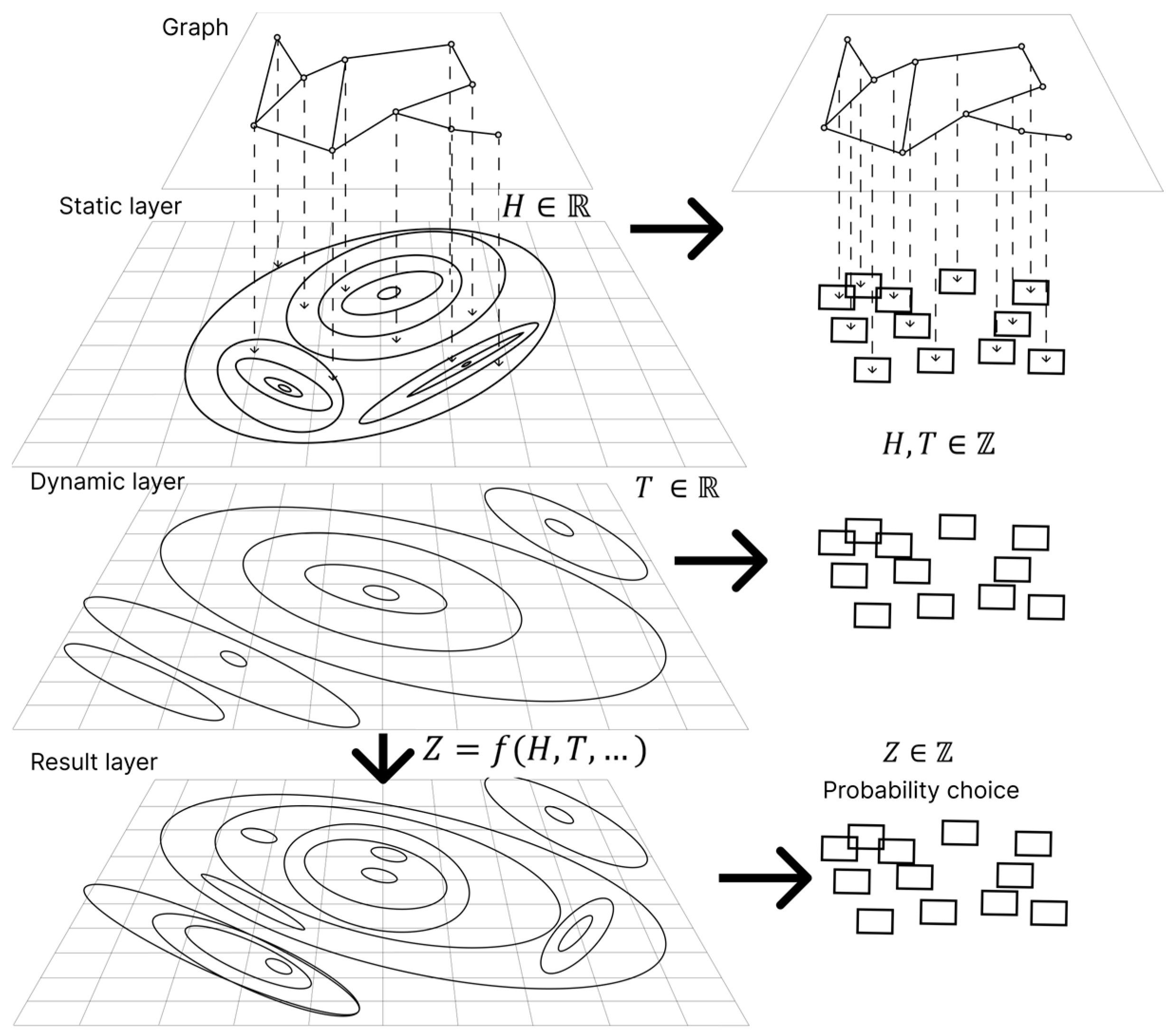
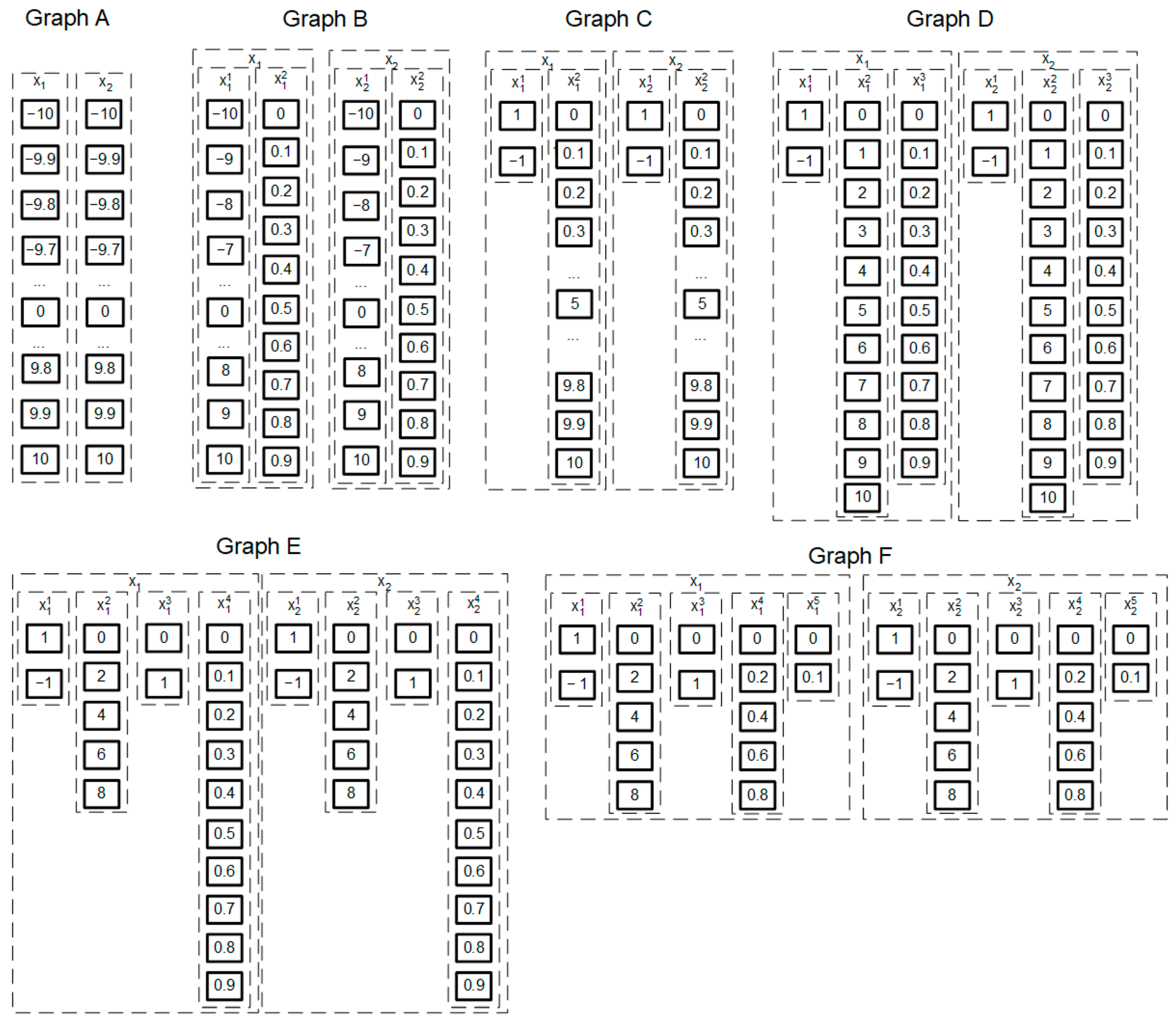

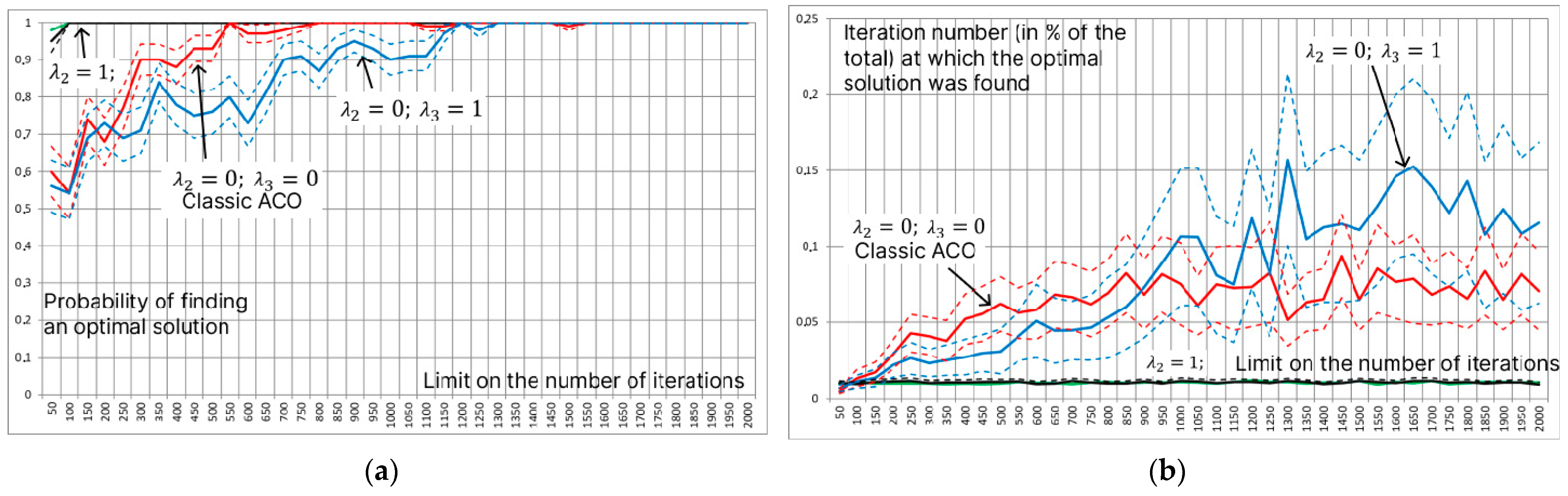
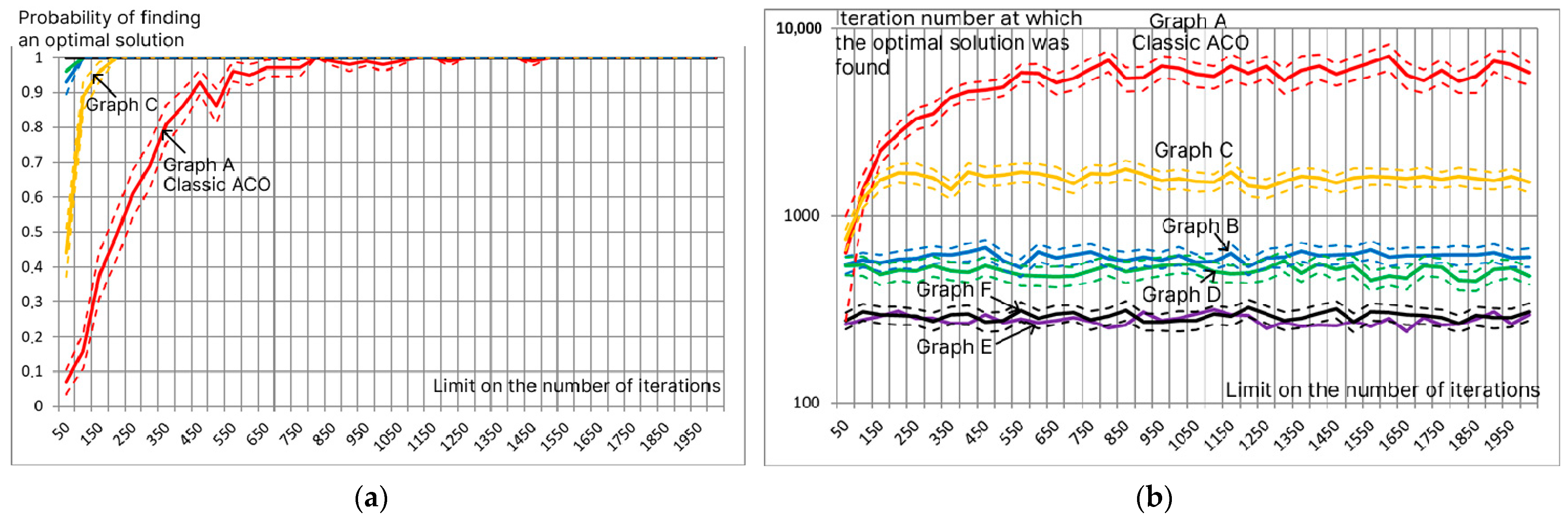
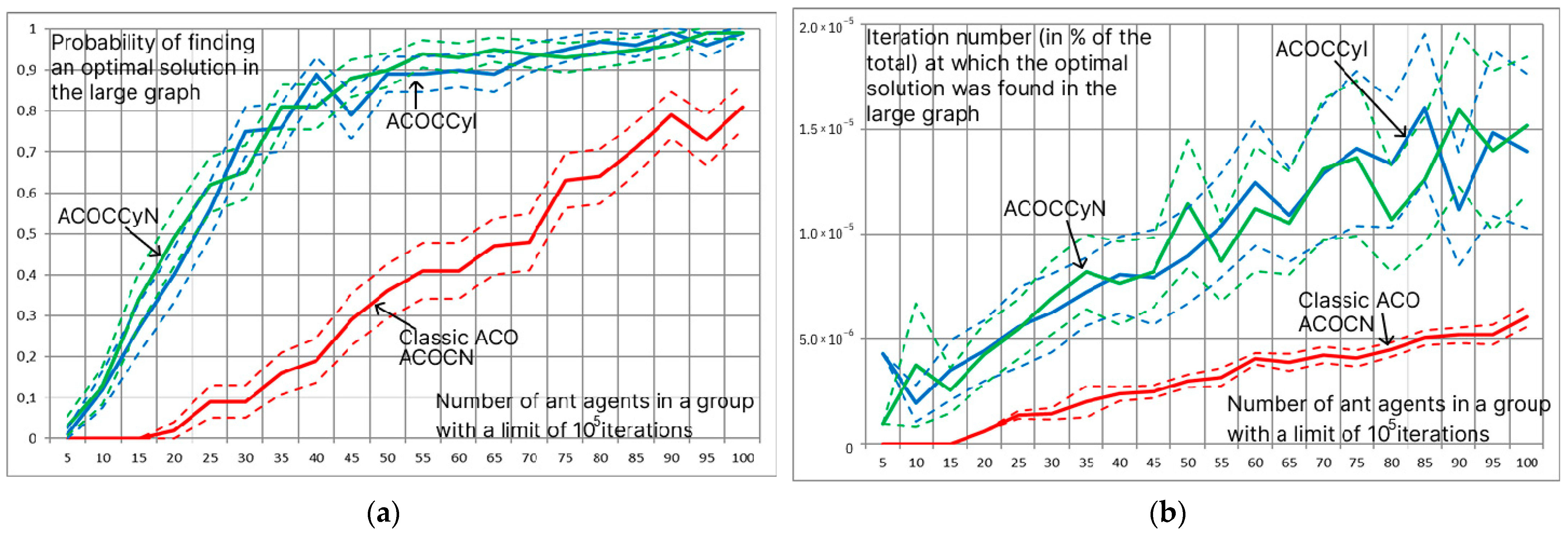
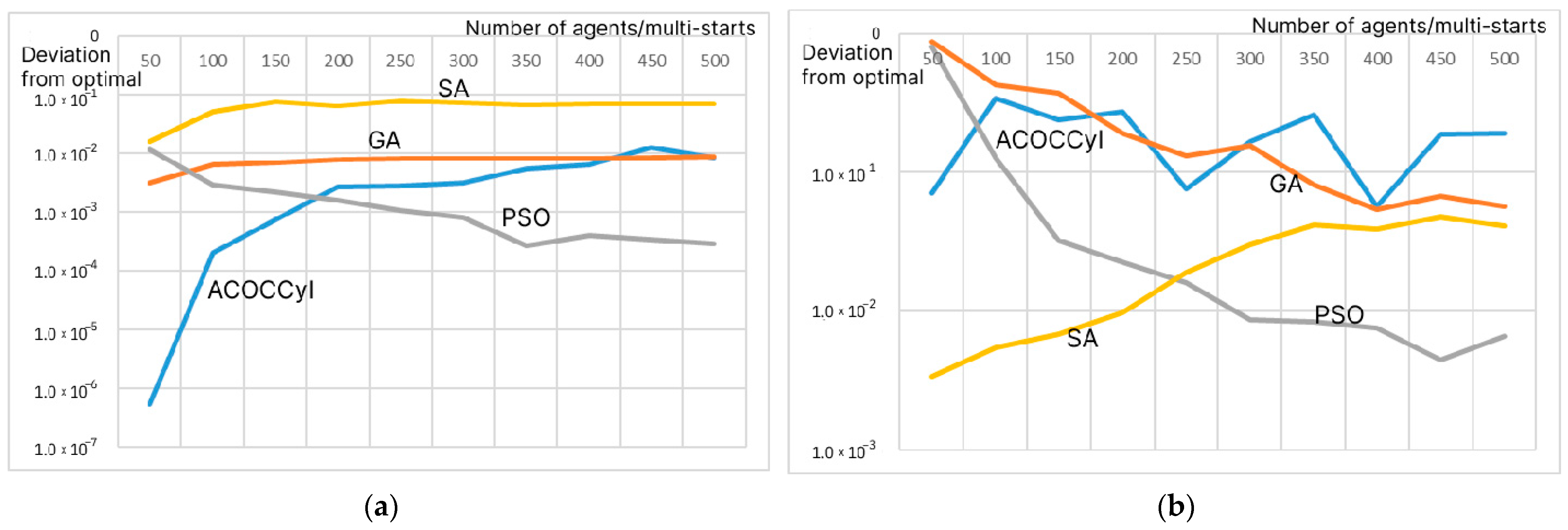

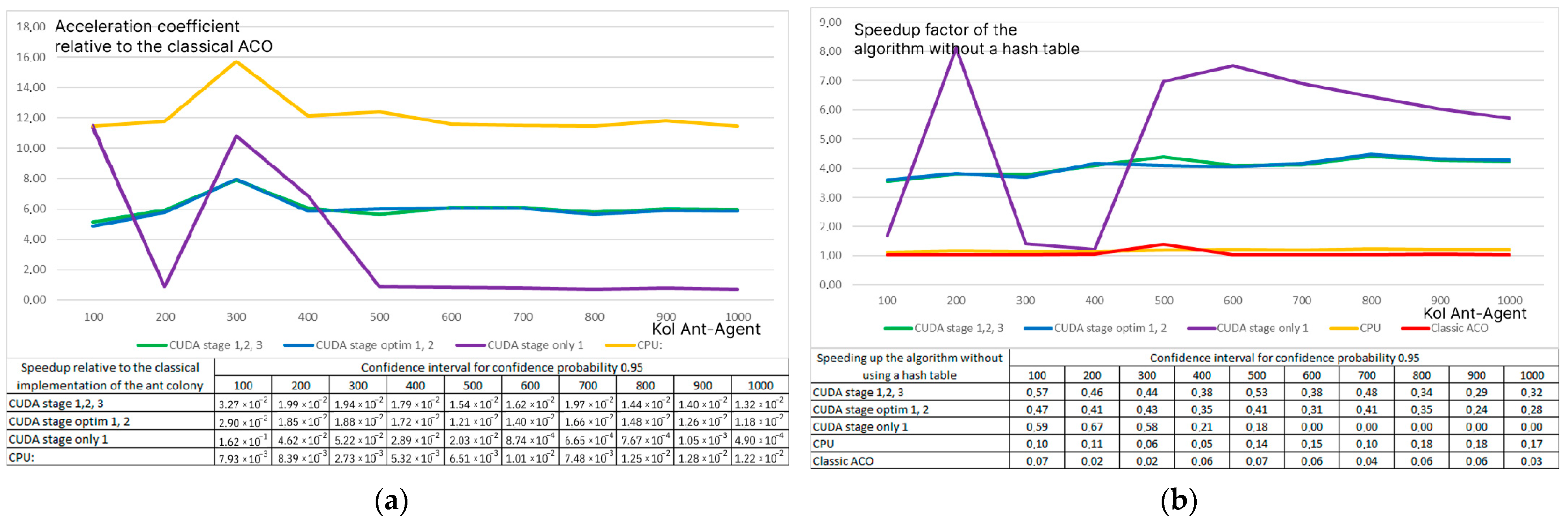
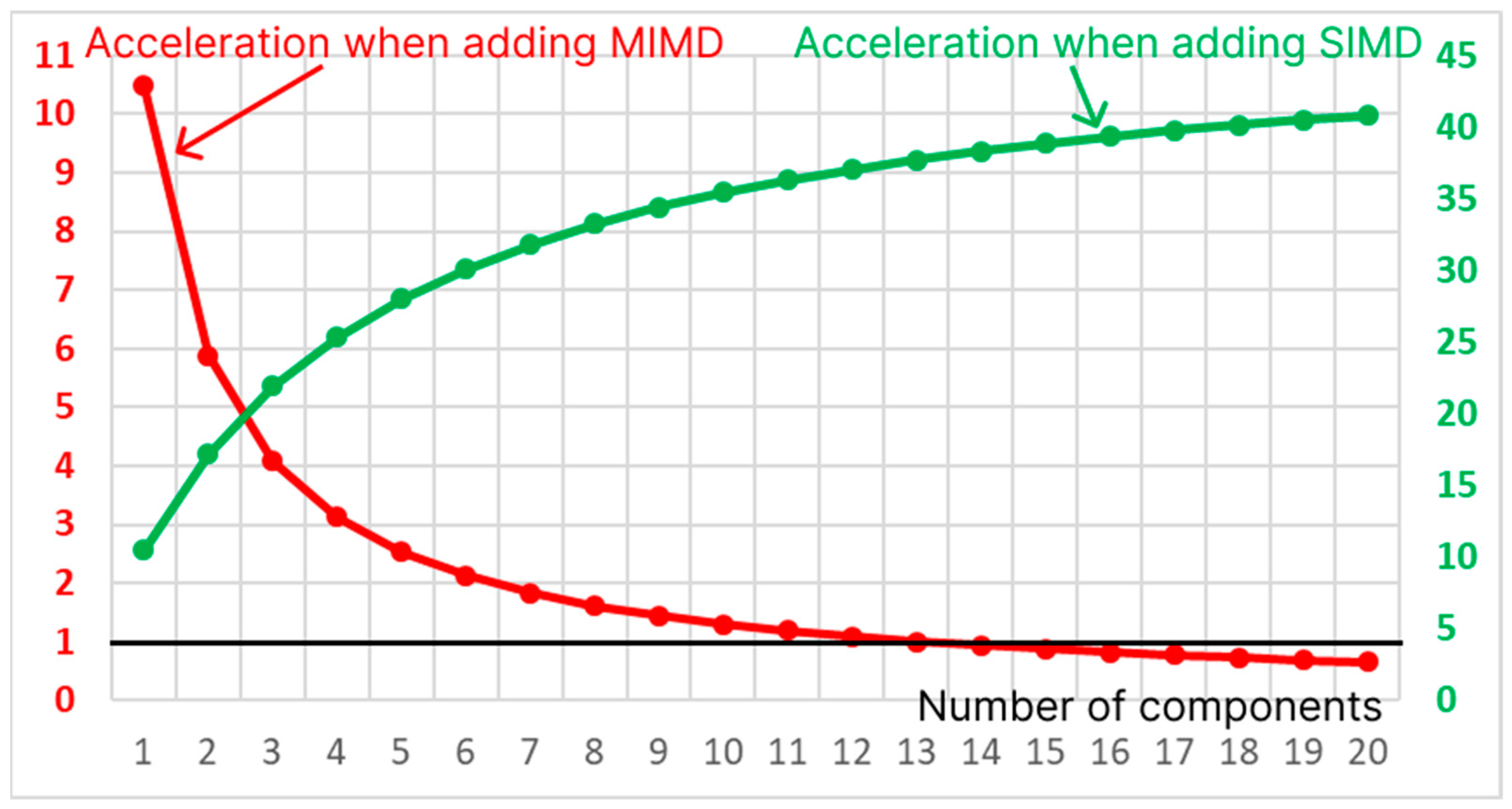
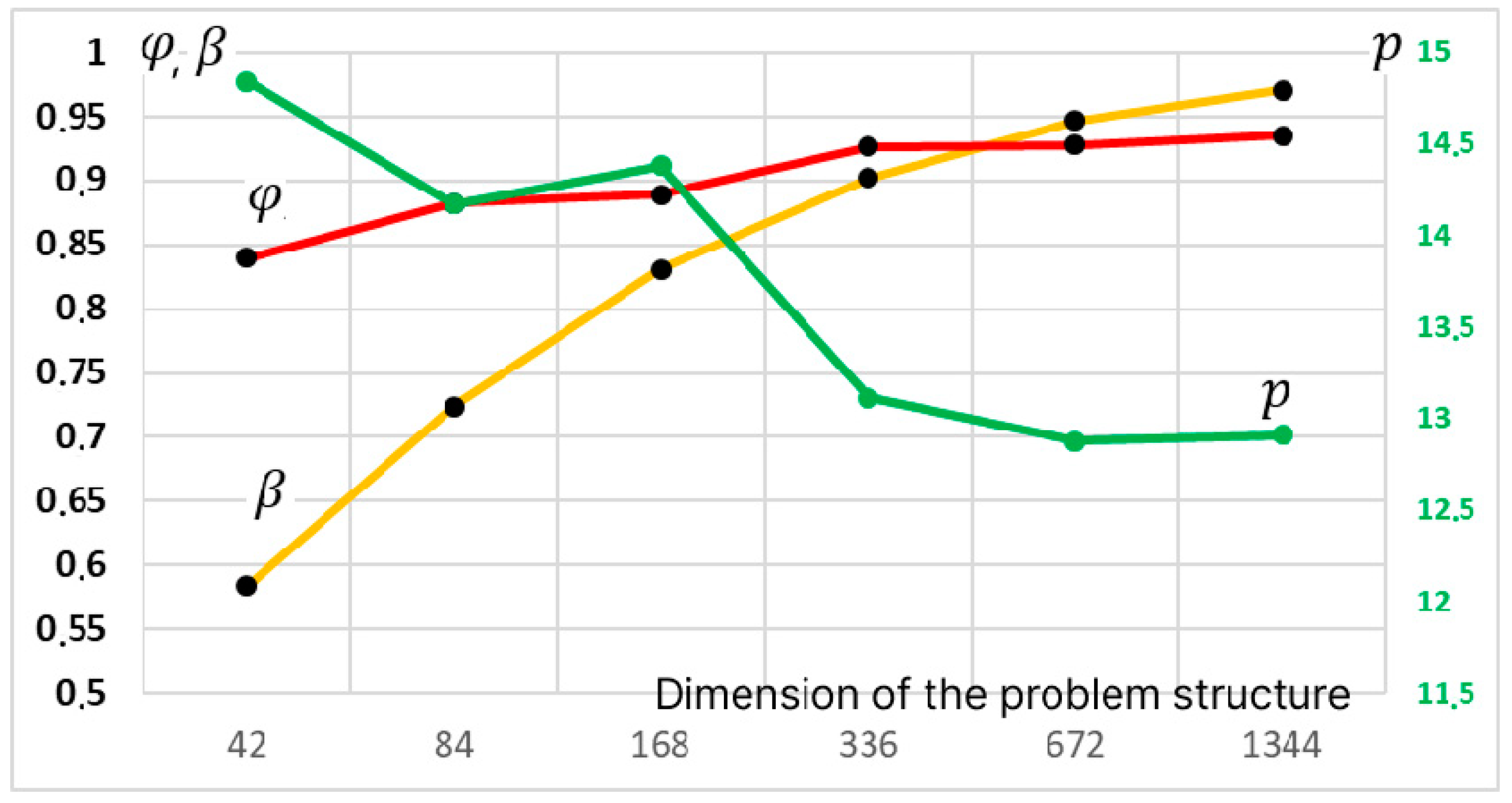
Disclaimer/Publisher’s Note: The statements, opinions and data contained in all publications are solely those of the individual author(s) and contributor(s) and not of MDPI and/or the editor(s). MDPI and/or the editor(s) disclaim responsibility for any injury to people or property resulting from any ideas, methods, instructions or products referred to in the content. |
© 2025 by the authors. Licensee MDPI, Basel, Switzerland. This article is an open access article distributed under the terms and conditions of the Creative Commons Attribution (CC BY) license (https://creativecommons.org/licenses/by/4.0/).