Article

Multi-Vehicle Collision Avoidance by Vehicle Longitudinal Control Based on Optimal Collision Distance Estimation

1
Department of Intelligent Robot Engineering, Pukyong National University, Busan 48513, Republic of Korea
2
Department of Mechatronics Engineering, Daelim University, Gyeonggi 13916, Republic of Korea
3
Graduate School of Data Science, Kyungpook National University, Daegu 41566, Republic of Korea
4
Department of Control and Instrumentation Engineering, Pukyong National University, Busan 48513, Republic of Korea
*
Authors to whom correspondence should be addressed.
These authors contributed equally to this work.
Mathematics 2025, 13(8), 1283; https://doi.org/10.3390/math13081283
Submission received: 5 March 2025 / Revised: 9 April 2025 / Accepted: 12 April 2025 / Published: 14 April 2025
(This article belongs to the Section E2: Control Theory and Mechanics)

Abstract

:
This paper proposes a collision avoidance method for vehicle longitudinal velocity control based on multi-vehicle collision distance estimation. The method begins by estimating the position and shape of object vehicles with collision risk using environmental sensors. The collision point is identified from the object vehicle’s surface, and a Kalman filter is applied for accurate estimation. The optimal collision distance is then determined by evaluating the collision risk at the identified point. A longitudinal control technique, incorporating the optimal collision distance and time gap, is employed to implement the collision avoidance system. The proposed method was validated through scenario-based simulations involving multi-vehicle collision avoidance, which were implemented in an environment combining ROS and the MORAI simulator, along with comparative experiments. Comparative studies with conventional vehicle center-based approaches demonstrated that the proposed surface-based collision point method significantly enhances collision avoidance performance. While the conventional method led to a collision between the ego and object vehicles, the proposed method successfully avoided the collision by maintaining a separation of about 3.6 m, demonstrating its feasibility and reliability.

1. Introduction

With recent advancements in autonomous driving systems, extensive research has focused on enhancing collision avoidance capabilities [1]. Accurate collision risk assessment and obstacle avoidance are critical for autonomous vehicle safety. This requires precisely estimating potential collision points using onboard sensors such as cameras, light detection and ranging (LiDAR), and radio detection and ranging (radar) [2,3,4]. Collision risk can be evaluated through the relative longitudinal acceleration between the target and ego vehicles during lane changes [5]. Moreover, by predicting surrounding vehicle movements based on lane information, lateral position, and velocity, autonomous systems can further mitigate collision risks [6]. Vehicle data such as position, velocity, and acceleration also enable trajectory prediction for collision avoidance [7,8]. Recently, deep learning techniques have been extensively studied to improve the prediction of potential collisions [9,10], while rapid evasive maneuvers can be achieved through direct actuator control [11].
Accurate object detection and localization are fundamental to effective collision avoidance. Advancements in computer vision, powered by deep learning, have significantly improved the detection of object type and shape [12]. Range sensors, such as LiDAR and radar, have been well developed for detecting the location and shape of object vehicles in two- and three-dimensional environments through point cloud clustering [13]. Additionally, research has focused on enhancing the accuracy of size and location detection within areas of interest by fusing vision sensor data—effective for object recognition—with range sensor data, which excels at capturing spatial and geometric information [14,15,16]. By leveraging the strengths of each sensor for multi-object tracking and integrating deep neural networks (DNNs), both accuracy and processing velocity have been improved [17,18]. Recently, studies have explored estimating vehicle locations using data received from communication systems, such as vehicle-to-vehicle (V2V) networks, to enhance object detection around the ego vehicle [19,20].
As stated above, collision avoidance technology should be implemented through autonomous vehicle control, relying on object estimation and risk assessment of potential collisions. To achieve this, a collision may be avoided through longitudinal and lateral control by utilizing vehicle information of the target vehicle as a basis for the autonomous vehicle [21,22]. Alternatively, by predicting the movement of the target vehicle, a potential risk area can be estimated and a path to avoid it in real time can be created to avoid collisions [23,24,25]. Recently, many studies have been conducted on collision avoidance control strategies using model predictive control (MPC). Since MPC has the advantage of being able to directly consider constraints, optimal control is possible according to the situation. Control for collision avoidance can be designed, such as MPC that predicts the dynamic movement of the target vehicle [26], MPC using the vehicle yaw rate to improve posture safety [27], and MPC for highway driving safety and rear collision avoidance [28]. Moreover, to solve the problem of MPC of a linear time-varying system modeled by a real vehicle system, MPC can be used to compensate for the uncertainty of the time-varying system by optimizing it like a linear time-invariant system and applying the compensation principle to avoid vehicle collisions between lane movements [29]. In addition, a winding road distance comparator (WRDC) has been proposed to improve lane tracking control performance through a compensator that ensures that lane tracking errors are reduced to zero for accurate lane tracking control for collision avoidance [30]. Also, safe driving can be achieved by applying backstepping sliding mode control to avoid collisions based on decision making and motion control [11].
Intersection environments, particularly unsignalized intersections, present a significant challenge for collision avoidance due to the difficulty in predicting vehicle trajectories and driver intentions. This complexity is further amplified when multiple vehicles approach the intersection simultaneously [31]. To address this issue, researchers have explored path prediction techniques that consider driver behavior and target vehicle operation [32]. Sensors attached to the target vehicle can estimate the dynamic movement of vehicles entering an intersection and avoid collisions based on their position relative to the ego vehicle [33,34]. By utilizing a dynamic Bayesian network (DBN) to predict vehicle states based on the position, velocity, and acceleration of vehicles entering an intersection, contextualized longitudinal controls such as deceleration and emergency braking can be applied to avoid collisions [35]. In addition, V2V and vehicle-to-infrastructure (V2I) communication technologies can be utilized to avoid collisions based on the relative positions of vehicles in an intersection environment [36]. The technologies mentioned above have been used to predict the state and position of a single vehicle entering an intersection and successfully avoid a collision [35,36]. For unsignalized intersections, multi-object estimation can be an effective method because multiple vehicles can enter at the same time [33]. These intersection collision risk determination and collision avoidance studies have solved the problem by calculating the distance between vehicles based on global positioning system (GPS) sensor points and vehicle center points [33,35,36]. Moreover, recent studies on learning-based approaches for collision avoidance at unsignalized intersections have demonstrated flexible decision making in complex and uncertain traffic environments [37,38]. However, while these studies have demonstrated meaningful results for collision avoidance at unsignalized intersections, further refinements in accurately estimating collision points in complex multi-vehicle environments and enhancing the robustness of collision risk assessment under unpredictable environments would be beneficial.
To address these refinements, this paper proposes a novel collision avoidance system that identifies and estimates optimal collision points for multiple vehicles. At unsignalized intersections, the system estimates collision points on the surface of object vehicles using a Kalman filter and continuously applies a geometric approach to calculate the minimum distance between vehicle surfaces, enabling more accurate and adaptive spatial assessment than conventional center-point methods. Unlike conventional approaches that focus on single-vehicle environments, by supporting multi-object environments, the method ensures optimal collision point and distance identification, even in complex traffic interactions. The proposed approach is validated through scenario-based simulations, demonstrating that the integration of precise collision point estimation with a longitudinal control strategy enables the implementation of a high-performance collision avoidance system that is both stable and responsive. The main contributions of this study are as follows:
  • Estimation of collision points on vehicle surfaces for collision avoidance.
  • Identification and estimation of optimal collision points for multiple vehicles.
  • Comparative experimental validation of collision avoidance systems based on estimated collision points.

2. Vehicle Collision Point Estimation

The proposed collision avoidance system applies optimal longitudinal control by estimating the collision point of the vehicle and identifying the collision point even in multi-vehicle environments, as illustrated in Figure 1. First, recognition, detection, and collision risk assessment of the object vehicle are required to estimate the collision point. This is because the collision risk with the ego vehicle can be calculated based on the size and shape of the object estimated through object recognition and detection [4]. To estimate the size and shape of object vehicles, previous studies have utilized object detection techniques based on onboard sensors such as LiDAR, radar, camera, and GPS. Object detection using onboard sensors involves estimating the optimal enclosing shape of discrete point sets, often through convex hulls or polygonal approximations, to infer object size and orientation. Among various methods, the L-shape algorithm combined with data sampling techniques enables robust and reliable detection [39]. Alternatively, communication technologies such as V2V can be used to receive information about the positions and types of object vehicles surrounding the ego vehicle [19]. Based on the estimated position, size, and shape of the object vehicles obtained from object detection techniques, the collision risk is assessed to determine whether a potential collision with the ego vehicle exists [2]. Thus, the proposed method improves the accuracy of collision risk assessment by estimating the collision point from the precise outline of the object vehicle rather than its center point.
The outline of the vehicle can be estimated using an approach that considers it to be a two-dimensional geometric shape based on parameters such as overall width and overall length [3]. Using vehicle parameters relative to the vehicle’s center point, the vertices of the vehicle can be estimated and connected to form a two-dimensional geometric shape. The two-dimensional geometric shape in the form of a rectangle is defined as the vehicle surface, and the minimum distance point ( M ) estimated from each surface. Finding the minimum distance point between the ego vehicle surface and the object vehicle surface is equivalent to finding the distance between the two closest points on the two-dimensional geometric shapes. This method can be calculated using a formula that determines the distance between the edges of shapes [40]. By calculating all relative distances between the two shapes using vector projection, the point with the shortest relative distance can be identified as the minimum distance point between the vehicles [3,26]. It is crucial to continuously estimate the surface as the vehicle follows curved paths, such as intersections, to accurately determine the minimum distance point. The homogeneous coordinate system enables continuous surface estimation by rotating the surface according to the current heading of the vehicle.
X Y 1 = c o s θ s i n θ X o f f s i n θ c o s θ Y o f f 0 0 1 X Y 1
where
X o f f = X 0 X 0 c o s θ + Y 0 s i n θ , Y o f f = Y 0 X 0 s i n θ Y 0 c o s θ
where X and Y are transformed coordinates and θ represents the vehicle’s current heading. X o f f and Y o f f are translation offsets. X 0 and Y 0 are the center of rotation, equivalent to the vehicle’s center point. X and Y denote the vehicle’s current position. Thus, by rotating the vehicle surfaces using homogeneous coordinates, we can achieve a more accurate estimation of the minimum distance between vehicles. At the minimum distance point, points on the ego vehicle’s and object vehicle’s surfaces are defined as
M e = [ M e , x M e , y ] , M o = [ M o , x M o , y ]
where M e and M o are the estimated minimum distance points on the ego vehicle and object vehicle, respectively. M e , x and M e , y denote the x- and y-coordinates of the ego vehicle’s surface, while M o , x and M o , y denote the x- and y-coordinates of the object vehicle’s surface. Figure 2 shows the method for estimating M e and M o , representing the minimum distance points with the shortest distance between the ego and object vehicle surfaces. The surface is defined from the vehicle’s center point using the ego vehicle’s width α e and length β e , and the object vehicle’s width α o and length β o . This illustrates how each vehicle’s surface is oriented accurately using homogeneous coordinates based on the vehicle parameters and how the minimum distance point is continuously estimated through geometry-based vector projection.
To estimate the collision point from the minimum distance point, M , the state vectors of the ego vehicle and the object vehicle are defined as follows:
X e = M e , x M e , y M ˙ e , x M ˙ e , y T , X o = M o , x M o , y M ˙ o , x M ˙ o , y T
where X e and X o are the x- and y-coordinates of the minimum distance points and the relative velocities of these coordinates for the ego vehicle and the object vehicle. For accurate data estimation, a motion model can be used to represent the motion of both the ego vehicle and the object vehicle within a discrete-time state-space framework. To design a discrete-time state-space model, the ego vehicle state vector X e and the object vehicle state vector X o can be expressed as state vectors X k at time k as follows:
X k + 1 = Φ X k + w k y k = C X k + v k
where
Φ = 1 0 Δ t 0 0 1 0 Δ t 0 0 1 0 0 0 0 1 , C = 1 0 0 0 0 1 0 0 0 0 1 0 0 0 0 1 , w k N ( 0 , Q k ) , v k N ( 0 , R k ) .
where X k denotes the state vector at time k . y k denotes the measurement vector. Φ is the constant velocity model and Δ t denotes the time interval. This model assumes that the vehicle maintains a uniform velocity during each time step Δ t and updates its position based on the current velocity. Due to its simplicity and effectiveness, the constant velocity model is widely adopted in object tracking and vehicle motion prediction [2]. C is defined as the identity matrix to extract the minimum distance point from the state vector while filtering out sensor noise. w k is the system noise and v k is the measurement noise from sensor data. Q k and R k are Gaussian-form covariance matrices [16].
Using the designed discrete-time state-space model, a Kalman filter (KF) is applied to estimate the minimum distance points of the ego vehicle and the object vehicle with the sensor data noise removed [41].
(a) Prediction:
X ^ k | k 1 = Φ X k 1 | k 1 P ^ k | k 1 = Φ P k 1 | k 1 Φ T + Q k ,
(b) Correction:
K K F = P ^ k | k 1 C k T ( C k P ^ k | k 1 C k T + R k ) k 1 X ^ k | k = X ^ k | k 1 + K K F ( y k C k X ^ k | k 1 ) P ^ k | k = ( I K K F C k ) P ^ k | k 1
where X ^ k | k 1 denotes the predicted state estimate and P ^ k | k 1 denotes the predicted error covariance. K K F is the optimal Kalman gain, X ^ k | k denotes the updated state estimate and P ^ k | k denotes the updated covariance estimate. I is the identity matrix.
By applying a Kalman filter to the measurement models of the ego vehicle and the object vehicle, it is possible to estimate the point at which the collision risk between the ego vehicle and the object vehicle is the highest, as well as the covariance of this collision point. Consequently, the collision point X ^ e and its covariance P ^ e for the ego vehicle can be estimated, along with the collision X ^ o and its covariance P ^ o for the object vehicle.

3. Multi-Vehicle Collision Point Identification

The estimation method for the single-vehicle collision point, as described in Section 2, can be extended to estimate the collision points for multiple object vehicles. For multi-vehicle collision environments, the collision point and covariance for the ego vehicle can be denoted as X ^ e ( i ) and P ^ e ( i ) , respectively. Similarly, the collision point and covariance for each object vehicle are represented as X ^ o ( i ) and P ^ o ( i ) , where i N i = { 1 , 2 , , n i } , and n i is the number of object vehicles. Importantly, X ^ e ( i ) accounts for the variation in the estimated collision point on the ego vehicle’s surface depending on the position of each object vehicle, enabling accurate collision risk assessment even in complex environments.
To identify the collision point with the highest collision risk among multiple object vehicles, the Mahalanobis distance D ( i ) · , · can be calculated for each vehicle. The Mahalanobis distance provides a probabilistic measure of similarity by incorporating the covariance structure of the data, making it well suited for assessing collision risk and computing optimal collision distances. This approach is particularly effective as it accounts for uncertainty in vehicle state estimation and spatial distribution. The Mahalanobis distance, which incorporates the covariance P ^ obtained from the Kalman filter, is computed as follows:
D ( i ) ( X ^ e ( i ) , X ^ o ( i ) ) = X ^ e ( i ) X ^ o ( i ) T P ^ e ( i ) + P ^ o ( i ) 1 X ^ e ( i ) X ^ o ( i ) .
The value of D is calculated for each object vehicle, and the collision risk between the ego vehicle and multiple object vehicles can be assessed by comparing these values. Thus, it is possible to estimate the optimal collision distance, indicating the point of highest collision risk for the ego vehicle.
D * = arg min i D ( i ) · , · .
By calculating the optimal collision distance D * , it is possible to obtain the distance information corresponding to the highest collision risk for the ego vehicle, which can then be used as a parameter for designing a longitudinal control strategy for collision avoidance. Figure 3 shows X ^ e ( i ) , P ^ e ( i ) , X ^ o ( i ) , P ^ o ( i ) , D, and D * for the collision points on the ego and object vehicles’ surfaces. It can be observed that as the ego vehicle enters the intersection, it calculates the collision distances with five object vehicles and identifies the optimal collision distance for the fourth object vehicle, which has the highest collision risk. Rather than estimating the minimum distance between the ego and object vehicles based on their center points, a more precise assessment of collision risk can be achieved by estimating the minimum distance point using the vehicle surface and filtering sensor noise through a Kalman filter. Even in multi-object-vehicle environments at intersections, the Mahalanobis distance-based optimal collision distance enables the identification of the most critical threat to the ego vehicle, thereby facilitating the design of an effective collision avoidance control strategy.

4. Optimal Longitudinal Control with Time Gap

If there is no risk of collision, the ego vehicle is designed to follow the desired acceleration based on the longitudinal vehicle model [42]. The longitudinal vehicle model is hierarchically structured with upper- and lower-level controllers. The upper-level controller determines the desired acceleration for the vehicle, while the lower-level controller adjusts the throttle and brake to achieve this desired acceleration. This design allows for simplification in tracking the desired acceleration under certain assumptions, as described below:
τ V x ¨ + V x ˙ = V x d ˙
where τ denotes a constant time delay, typically set to 0.5 s, V x is the current velocity of the ego vehicle, and V x d is the desired longitudinal velocity. This longitudinal vehicle dynamics model has been widely adopted in autonomous driving research, ranging from early studies to state-of-the-art approaches, and continues to serve as a fundamental framework for velocity control [43]. The velocity control can be described as follows:
x ˙ = 0 1 0 1 τ x + 0 1 τ u
where x = V x V ˙ x T denotes the state vector, and u denotes the desired longitudinal acceleration, V ˙ x d . Although one of the eigenvalues of the system matrix is zero, the vehicle longitudinal dynamics can still be stabilized via state-feedback control since the pair of the system matrix and control matrix is controllable [44]. We assume that the state-feedback controller u ( k ) is applied as follows:
u ( k ) = K L Q R ( x d ( k ) x ( k ) )
where x d denotes the state reference for trajectory tracking and x denotes the output states of the vehicle. A linear–quadratic regulator (LQR) is employed for longitudinal control in trajectory tracking to obtain the optimal control gain K L Q R . The state-feedback optimal control gain K L Q R for the vehicle’s longitudinal controller is designed using LQR, which minimizes the linear quadratic cost function:
J = k = 0 ( x ( k ) T Q L Q R x ( k ) + u ( k ) T R L Q R u ( k ) )
where Q L Q R and R L Q R are weighting coefficients for the LQR controller design. Solving the discrete-time algebraic Riccati equation (DARE), the ego vehicle is controlled using the LQR to track the desired longitudinal acceleration a L Q R .
To avoid collisions, a longitudinal control strategy is implemented that considers the current velocity of the ego vehicle using the time gap (TG). This longitudinal control strategy calculates the linear longitudinal acceleration of the ego vehicle using D * and the time gap to maintain a safe interval for collision avoidance. First, a spacing error is defined to maintain a safe distance from the object vehicle:
ρ = D * + h V x
where V x denotes the longitudinal velocity of the ego vehicle and h denotes the time gap. ρ denotes the spacing error. This is the desired distance from the object vehicle. It can be adjusted according to h. Using the spacing error ρ from the object vehicle, the desired longitudinal acceleration of the ego vehicle can be calculated as follows:
a T G = 1 h ( D ˙ * + λ ρ )
where λ is the relaxation factor for the time gap and 0 < λ . With this control law, it can be shown that the spacing errors of successive ρ values are independent of each other. Equation (15) can be differentiated to obtain
ρ ˙ = D ˙ * + h V ˙ x .
Substituting for V ˙ x from Equation (16) into Equation (17) and assuming V ˙ x = a T G , the error dynamics for ρ are obtained as
ρ ˙ = λ ρ .
Thus, ρ is independent and is expected to converge to zero as long as λ > 0, demonstrating that the control formulation ensures stability and feasibility. This implies that the vehicle can be autonomously controlled, independently of the object vehicle or external factors, validating the reliability of the proposed control system.
When an object vehicle with potential collision risk is detected during driving, the velocity of the ego vehicle is adjusted using time-gap control to avoid a collision. In this approach, a L Q R and a T G are utilized to apply a context-appropriate acceleration as the desired longitudinal input for the ego vehicle, achieving effective collision avoidance.
Thus, the desired longitudinal acceleration, as the final control input, is given by
a * = min ( a L Q R , a T G ) .
This longitudinal control strategy enables collision avoidance in multi-object-vehicle environments at intersections, based on optimal collision distance estimation. The integrated collision avoidance system consists of several key components, including surface-based minimum distance point detection, a Kalman filter for sensor noise reduction, accurate collision point and distance estimation even in multi-object-vehicle environments, and Mahalanobis distance-based optimization for collision risk assessment, collectively forming a unified decision-control framework. These elements work together to provide robust performance, and the system has also demonstrated effectiveness in single-object-vehicle environments. Moreover, the method can be readily applied to commercial vehicles with onboard sensors, offering high applicability and reliability through a probabilistic optimization framework.

5. Experiment

To validate the proposed longitudinal control strategy for the ego vehicle, scenario-based simulations are conducted in the MORAI simulator, utilizing vehicle dynamics and custom sensor models. The MORAI simulator provides a safety verification process for the development and operation of autonomous driving systems, supporting ISO 26262 certification and Automotive Safety Integrity Level D (ASIL D) [45].

5.1. Experimental Setup

The MORAI simulator is integrated with the Robot Operating System (ROS) on a Linux-based Ubuntu 20.04 environment. Using the User Datagram Protocol (UDP) communication, ROS and the MORAI simulator are connected to exchange ego vehicle information, object vehicle information, and scenario and sensor data. Python 3.10 was utilized to control the ego vehicle within the simulation, and longitudinal and lateral control strategies were designed separately. The vehicle used in the simulation was a 2017 KIA Niro Hybrid, equipped with sensor systems such as LiDAR, a camera, and a GPS for autonomous driving. The simulation map represents an unsignalized intersection, where experiments were conducted. For an unsignalized intersection, a high-definition (HD) map of the real-world environment in the Daegu-Gyeongbuk Free Economic Zone in South Korea was created and set as the simulation map in the MORAI simulator. Figure 4 shows the paths of the ego vehicle and object vehicles in the scenario-based simulation conducted on the map of the real-world environment at the unsignalized intersection.

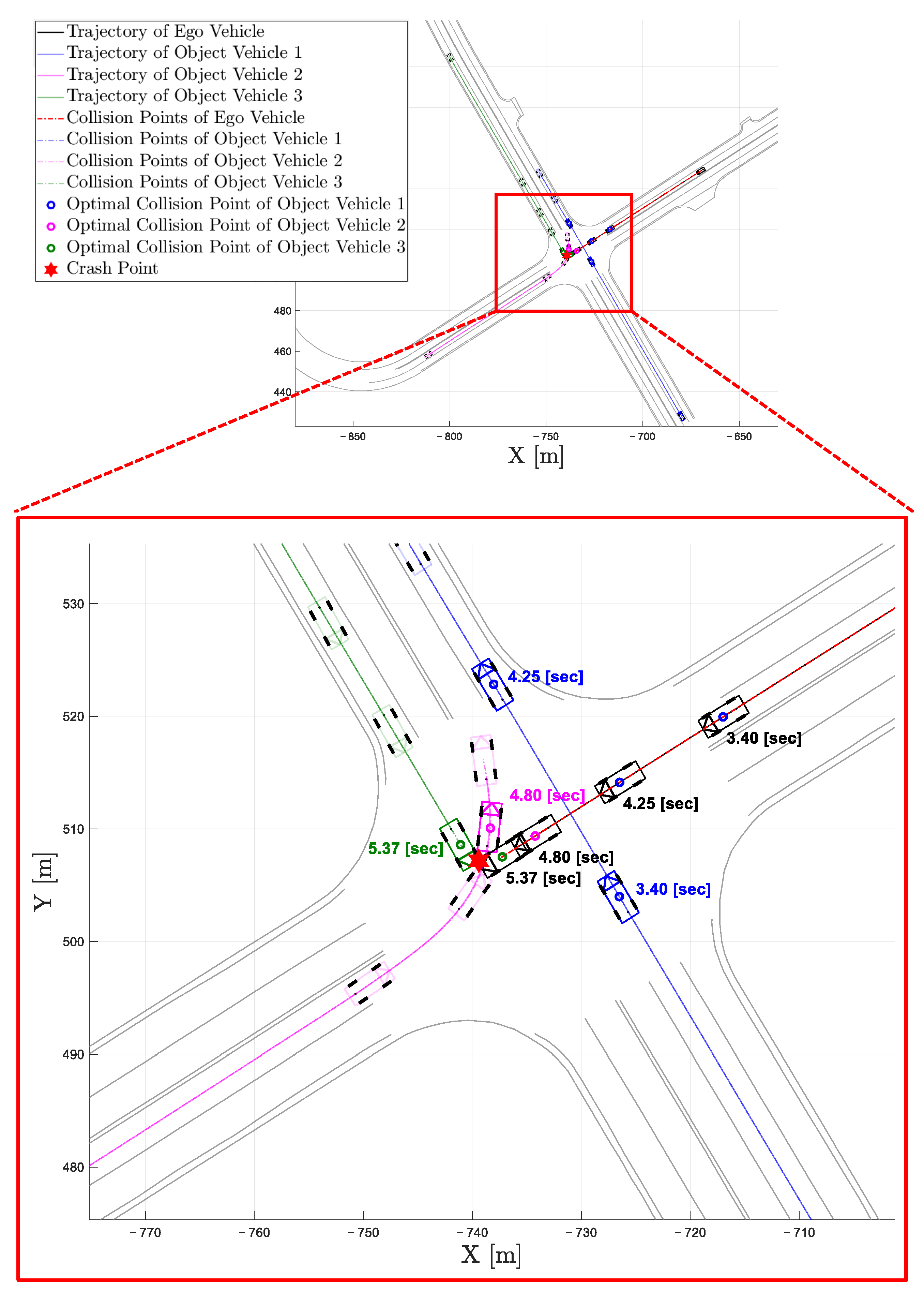
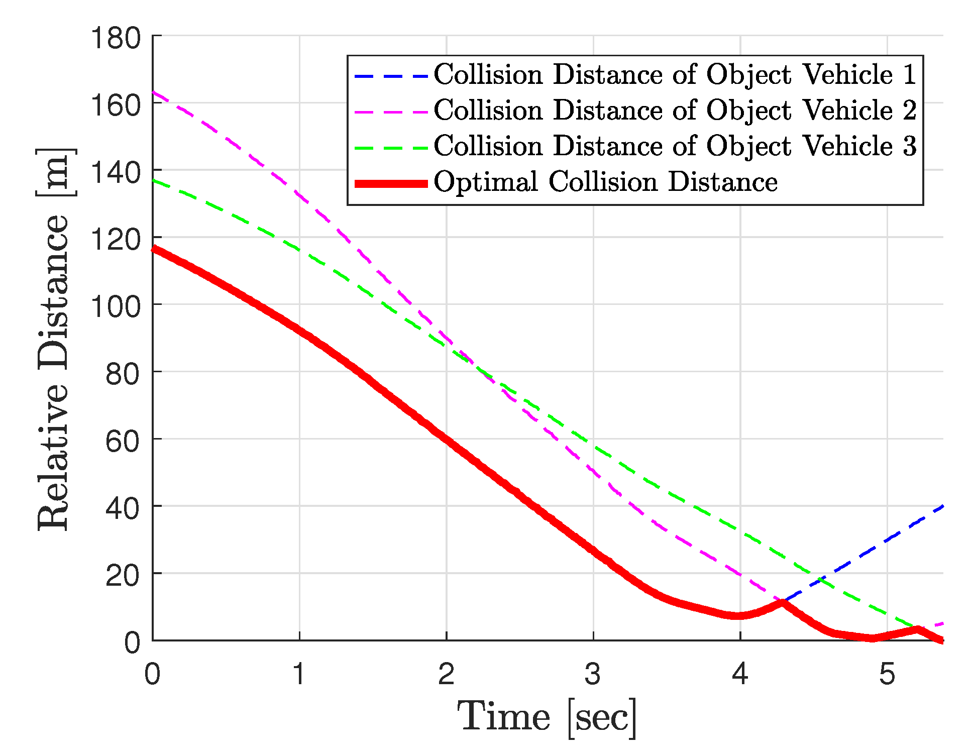
5.2. Scenario-Based Simulation

The scenario is a multi-object-vehicle scenario in which the ego vehicle and three object vehicles enter an unsignalized intersection at different speeds. The ego vehicle is driving along a straight longitudinal path, while the three object vehicles drive in the following sequence relative to the ego vehicle: from left to right (object vehicle 1), from the front to the right (object vehicle 2), and from right to left (object vehicle 3). The object vehicles are driving at speeds of 50 kph, 45 kph, and 40 kph, respectively. To replicate a realistic scenario, the object vehicles decelerate before entering the intersection. In particular, object vehicle 2 slows down further to drive a left turn at the intersection. Figure 5 shows the scenario-based simulation running in the MORAI simulator. The moments of highest collision risk for object vehicles 1 through 3 are illustrated as the ego vehicle is driving. (a) shows the highest collision risk for object vehicle 1, while (b) and (c) show the highest collision risks for object vehicles 2 and 3, respectively. The proposed ego vehicle longitudinal control strategy is validated in multi-object environments with two or more objects by calculating the optimal collision distance D * and applying the collision avoidance longitudinal control strategy, demonstrating both safety and feasibility in the scenario-based simulation.

5.3. Test Result

Figure 6 shows a top view of the trajectories of the ego vehicle and multiple object vehicles in the multi-object scenario, along with the HD map used for the test. This illustrates how the ego vehicle estimates the optimal collision distance D * to the object vehicle with the highest collision risk, while also estimating the collision points with multiple object vehicles. The positions of the ego vehicle and object vehicles were obtained using GPS sensors mounted on the vehicles, combined with object detection techniques. Based on the positional data, the surfaces of both the ego and object vehicles were estimated using their respective parameters. These estimated surfaces were utilized to visualize each moment of motion and the corresponding optimal collision distance over time. The optimal collision distance was first estimated for object vehicle 1, followed sequentially by object vehicle 2 and object vehicle 3. It is observed that the ego vehicle followed the prescribed path without collision with any of the object vehicles, enabled by longitudinal velocity control based on the optimal collision distance. Figure 7 shows the determination of the collision points for the multiple object vehicles and the corresponding collision distances. As the ego and object vehicles drove, D * was estimated from object vehicle 1 between 0 and 4.5 s, from object vehicle 2 between 4.5 and 5.8 s, and from object vehicle 3 from 5.8 s until the end of the scenario.
Figure 8a shows the slowing of the velocities of the object vehicles as they enter the intersection to simulate a realistic environment and Figure 8b shows the relative velocities between the ego vehicle and the object vehicles based on their velocities. In particular, it can be observed that object vehicle 2 drives at a reduced velocity while making a left turn at the intersection, then resumes its set velocity upon returning to the lane. Using D * , the ego vehicle’s desired longitudinal acceleration was determined by comparing two control values: a T G , which is for collision avoidance, and a L Q R , which facilitates tracking the desired speed in the absence of collision risks. This is shown in Figure 9a. As shown in Figure 7, from 4.5 s to 5.8 s, D * is estimated from object vehicle 2. This result of applying the value of a T G to the ego vehicle’s desired longitudinal acceleration to avoid a collision is shown. By applying this acceleration as the input to the ego vehicle, the vehicle decelerated and successfully avoided collisions with all object vehicles. It can be confirmed that the proposed longitudinal control strategy applied the appropriate acceleration as the desired longitudinal value. Figure 9b shows the ego vehicle’s velocity of the applied desired longitudinal acceleration value. The proposed control strategy demonstrates deceleration to avoid collisions with multiple object vehicles, followed by resuming a constant velocity to track the longitudinal path. As a result, this confirms the successful implementation of the longitudinal velocity control strategy for collision avoidance.

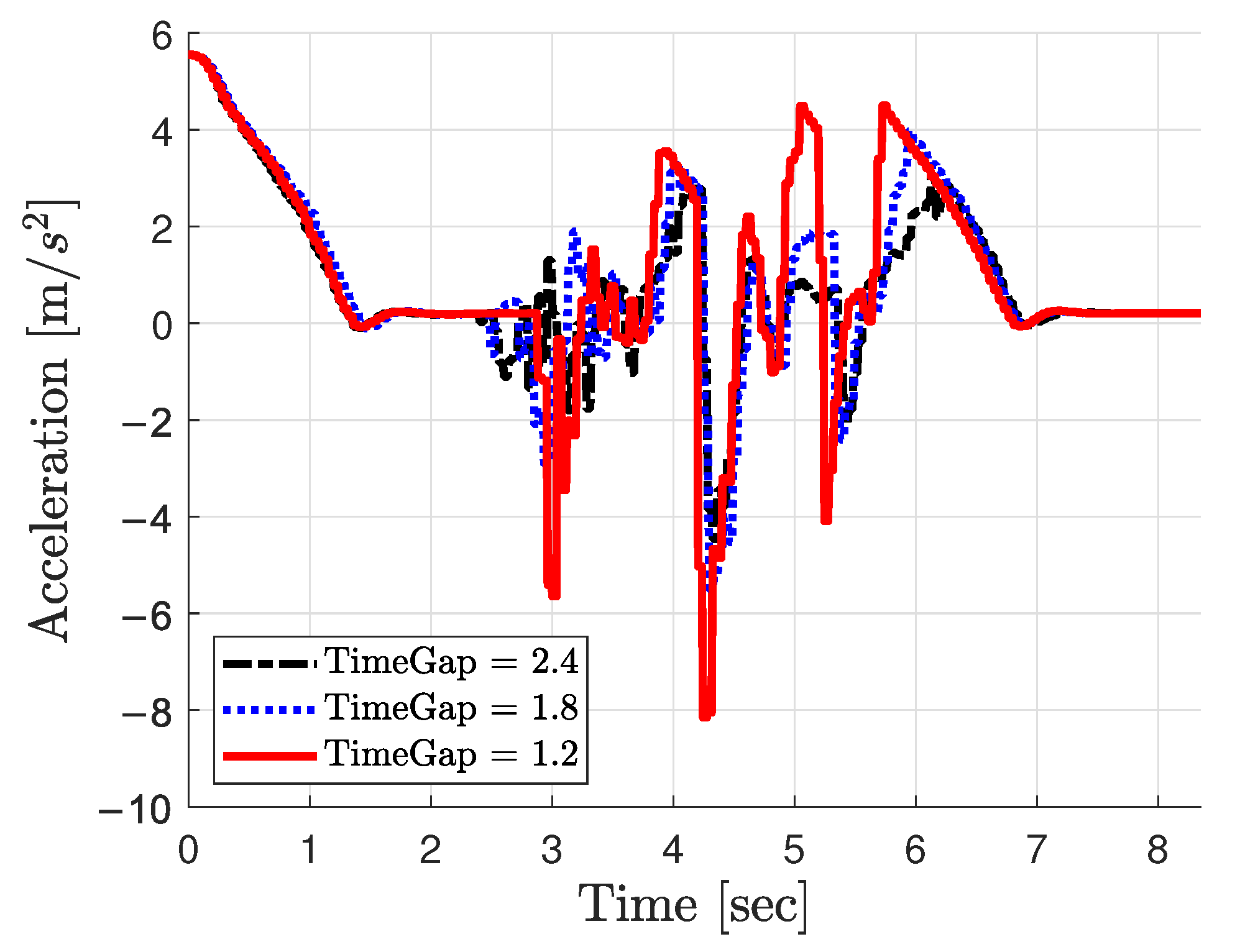
5.4. Experiment Varying Time-Gap Parameter

The time-gap parameter of the longitudinal velocity control strategy for collision avoidance is a human factor that can be adjusted for user convenience. This is because a larger time-gap parameter results in an increased spacing error, ρ . This means that a safe distance can be determined from a vehicle at risk of collision based on the optimal collision distance. By adjusting the time-gap parameter, it is possible to initiate deceleration early by setting a larger safety distance to prevent abrupt acceleration or deceleration of the vehicle. Alternatively, for a more flexible traffic flow, a narrow safety distance can be set, allowing for quicker acceleration and deceleration transitions. Therefore, the time-gap parameter enables the user to set an appropriate distance to avoid collisions with vehicles at risk, according to their preferences. Figure 10 shows the longitudinal acceleration control value a T G as the time-gap parameter is varied in the scenario-based simulation in Section 5.2. As the time-gap parameter increases, ρ becomes larger, resulting in earlier application of acceleration to avoid collisions with object vehicles and a smaller gradient in deceleration changes. However, as the time-gap parameter decreases, the spacing error ρ also decreases, leading to delayed acceleration application and a larger gradient in deceleration changes. It is significant that when the time-gap parameter is set to 1.2, the ego vehicle experiences an emergency-level deceleration due to rapid changes, but no collision occurs with the object vehicle, indicating a meaningful outcome.

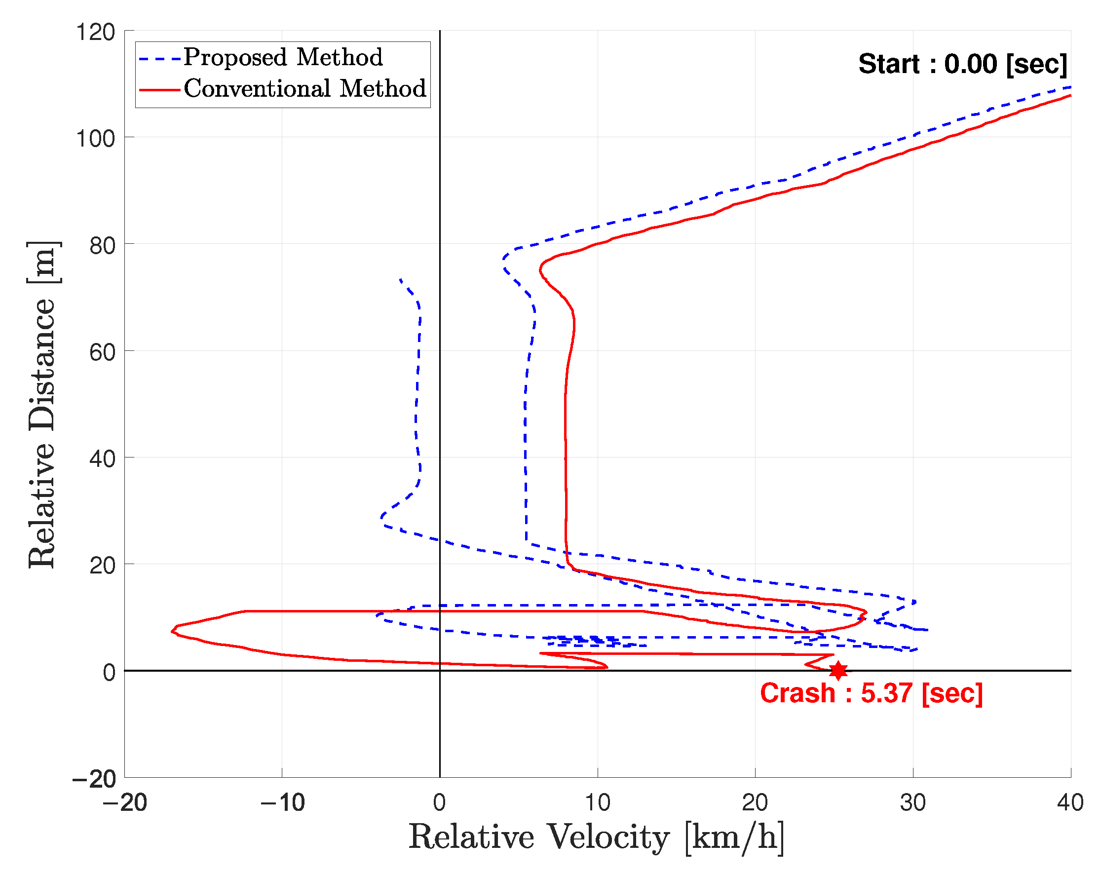
5.5. Comparison Experiment

To verify the effectiveness and feasibility of the proposed longitudinal control strategy, an additional experiment was conducted under different conditions within the same scenario environment. The modified condition was the collision point estimation method. In the initial experiment, the collision point and optimal collision distance were calculated based on the vehicles’ surfaces. However, calculating the collision point based on the center points of vehicles is also commonly used and can serve as an intuitive criterion. The feasibility of the proposed longitudinal control strategy is demonstrated by applying the optimal collision distance D * from the vehicle center and adjusting the time gap to compare with the existing method. The acceleration for longitudinal control is calculated by setting the time gap to 1.2 and experimenting in the same scenario. The acceleration calculated based on the optimal collision distance from the vehicle’s center point demonstrates a relatively lower performance in preparing for collision risks.
Figure 11 shows a top view of the trajectories of the ego vehicle and multiple object vehicles, along with the HD map, for the comparison experiment. It can be observed that the collision point and collision distance are estimated from the center points of both the ego and object vehicles. In this experiment, although the optimal collision distance was calculated from the center point of object vehicle 3, the distance between the vehicle surfaces was closer, leading to a collision. At the point of collision, referred to as the crash point, the estimated collision point from the vehicle surfaces coincides with the optimal collision distance, which reaches zero. Figure 12 shows the collision distance and the optimal collision distance from the surfaces of the ego and object vehicles in the comparison experiment. As described previously, due to the longitudinal acceleration calculated from the vehicle’s center point, the optimal collision distance between the surfaces of the ego vehicle and object vehicle 3 converged to zero, resulting in a collision. Figure 13 shows the desired longitudinal acceleration and velocity of the ego vehicle during the comparison experiment with the object vehicle. As the time-gap parameter decreases, the spacing error reduces, leading to delayed deceleration to avoid a collision with object vehicle 1. It is observed that in Figure 9a, deceleration is applied at 2.5 s, whereas in Figure 13a, it is applied at 3.2 s, resulting in delayed collision avoidance for object vehicle 1. Additionally, the variation in deceleration is more significant, indicating the occurrence of sharp deceleration, such as an emergency stop. In Figure 13b, the velocity of the ego vehicle decreases rapidly following sudden deceleration, resulting in a collision with the object vehicle as avoidance was unsuccessful.
The results of the collision avoidance experiment and the comparison experiment can be effectively interpreted when expressed in terms of relative distance and relative velocity rate. As shown in Figure 14, the proposed method avoided collisions with the object vehicles while maintaining a safe distance of 3.6764 m, without the relative distance reaching zero. In contrast, the comparison method resulted in a collision, as the relative distance reached zero at 5.37 s. The experimental results demonstrate that the proposed collision point identification method and the longitudinal collision avoidance control system for multiple object vehicles were effectively applied, validating their feasibility and reliability.

6. Conclusions

This paper proposed a collision avoidance system for longitudinal velocity control, incorporating multi-vehicle optimal collision distance estimation. Simulations were implemented in an environment combining ROS and the MORAI simulator, and comparative experiments were conducted. Scenario-based simulations at unsignalized intersections demonstrated the method’s effectiveness, as the ego vehicle successfully avoided collisions through longitudinal velocity control based on multi-vehicle collision point estimation. Comparative experiments with varying time-gap parameters further validated the approach’s feasibility and reliability. Although the proposed method demonstrated promising results, its validation has so far been limited to simulation environments. Future works will include experimental validation using a real vehicle to verify the practical applicability of the proposed approach. Furthermore, by enhancing prediction and estimation for both ego- and object vehicle surfaces, this control strategy can evolve into a more robust solution with integrated collision risk assessment. The proposed method holds potential for broad applications beyond commercial and autonomous vehicles equipped with onboard sensors, extending to intelligent mobility platforms such as robots and drones.

Author Contributions

Conceptualization, J.H.L. and W.Y.C.; methodology, Y.S.S. and W.Y.C.; software, J.H.L.; validation, J.H.L., Y.L. and W.Y.C.; formal analysis, J.H.L., Y.S.S. and W.Y.C.; investigation, J.H.L. and Y.L.; resources, W.Y.C.; data curation, J.H.L.; writing—original draft preparation, J.H.L.; writing—review and editing, J.H.L., Y.L. and W.Y.C.; visualization, J.H.L.; supervision, W.Y.C.; project administration, J.H.L., Y.L. and W.Y.C.; funding acquisition, Y.S.S. and W.Y.C. All authors have read and agreed to the published version of the manuscript.

Funding

This research was supported partly by the Technology Innovation Program (No. 20014121, Development of integrated Minimal Risk Maneuver technology for fallback system during autonomous Driving) funded By the Ministry of Trade, Industry & Energy (MOTIE, Republic of Korea), and partly by the National Research Foundation of Korea (NRF) grant funded by the Korea government (MSIT) (No. RS-2023-00213640, Accurate autonomous tracking control by unmatched disturbance compensator with reference re-design filter), and partly by the Technological Innovation R&D Program (S3430140) funded by the Ministry of SMEs and Startups (MSS, Republic of Korea).

Data Availability Statement

The datasets presented in this article are not readily available because the data are part of an ongoing study. Requests to access the datasets should be directed to wychoi@pknu.ac.kr.

Conflicts of Interest

The authors declare no conflict of interest.

References

  1. Fu, Y.; Li, C.; Yu, F.R.; Luan, T.H.; Zhang, Y. A Survey of Driving Safety with Sensing, Vehicular Communications, and Artificial Intelligence-Based Collision Avoidance. IEEE Trans. Intell. Transp. Syst. 2021, 23, 6142–6163. [Google Scholar] [CrossRef]
  2. Choi, W.Y.; Lee, S.H.; Chung, C.C. On-Road Object Collision Point Estimation by Radar Sensor Data Fusion. IEEE Trans. Intell. Trans. Syst. 2021, 23, 14753–14763. [Google Scholar] [CrossRef]
  3. Altendorfer, R.; Wilkmann, C. A new approach to estimate the collision probability for automotive applications. Automatica 2021, 127, 109497. [Google Scholar] [CrossRef]
  4. Choi, W.Y.; Yang, J.H.; Chung, C.C. Data-Driven Object Vehicle Estimation by Radar Accuracy Modeling with Weighted Interpolation. Sensors 2021, 21, 2317. [Google Scholar] [CrossRef]
  5. Lee, H.; Kang, C.M.; Kim, W.; Choi, W.Y.; Chung, C.C. Predictive risk assessment using cooperation concept for collision avoidance of side crash in autonomous lane change systems. In Proceedings of the 2017 17th International Conference on Control, Automation and Systems (ICCAS), Jeju, Republic of Korea, 18–21 October 2017; IEEE: Piscataway, NJ, USA, 2017; pp. 47–52. [Google Scholar]
  6. Kim, J.; Kum, D. CollisionRrisk Assessment Algorithm via Lane-Based Probabilistic Motion Prediction of Surrounding Vehicles. IEEE Trans. Intell. Trans. Syst. 2017, 19, 2965–2976. [Google Scholar] [CrossRef]
  7. Li, G.; Yang, Y.; Zhang, T.; Qu, X.; Cao, D.; Cheng, B.; Li, K. Risk assessment based collision avoidance decision-making for autonomous vehicles in multi-scenarios. Transp. Res. Part C Emerg. Technol. 2021, 122, 102820. [Google Scholar] [CrossRef]
  8. Ma, Y.; Dong, F.; Yin, B.; Lou, Y. Real-time risk assessment model for multi-vehicle interaction of connected and autonomous vehicles in weaving area based on risk potential field. Phys. A Stat. Mech. Its Appl. 2023, 620, 128725. [Google Scholar] [CrossRef]
  9. Noh, S. Decision-Making Framework for Autonomous Driving at Road Intersections: Safeguarding Against Collision, Overly Conservative Behavior, and Violation Vehicles. IEEE Trans. Ind. Electron. 2018, 66, 3275–3286. [Google Scholar] [CrossRef]
  10. Katrakazas, C.; Quddus, M.; Chen, W.H. A new integrated collision risk assessment methodology for autonomous vehicles. Accid. Anal. Prev. 2019, 127, 61–79. [Google Scholar] [CrossRef]
  11. He, X.; Liu, Y.; Lv, C.; Ji, X.; Liu, Y. Emergency steering control of autonomous vehicle for collision avoidance and stabilisation. Veh. Syst. Dyn. 2019, 57, 1163–1187. [Google Scholar] [CrossRef]
  12. Zou, Z.; Chen, K.; Shi, Z.; Guo, Y.; Ye, J. Object Detection in 20 Years: A Survey. Proc. IEEE 2023, 111, 257–276. [Google Scholar] [CrossRef]
  13. Wu, Y.; Wang, Y.; Zhang, S.; Ogai, H. Deep 3D Object Detection Networks Using LiDAR Data: A Review. IEEE Sens. J. 2020, 21, 1152–1171. [Google Scholar] [CrossRef]
  14. Zhao, X.; Sun, P.; Xu, Z.; Min, H.; Yu, H. Fusion of 3D LIDAR and Camera Data for Object Detection in Autonomous Vehicle Applications. IEEE Sens. J. 2020, 20, 4901–4913. [Google Scholar] [CrossRef]
  15. Ghasemieh, A.; Kashef, R. 3D object detection for autonomous driving: Methods, models, sensors, data, and challenges. Transp. Eng. 2022, 8, 100115. [Google Scholar] [CrossRef]
  16. Lee, S.H.; Choi, W.Y. Enhancing Object Estimation by Camera-LiDAR Sensor Fusion Using IMM-KF with Error Characteristics in Autonomous Robot Systems. IEEE Access 2024, 12, 197247–197258. [Google Scholar] [CrossRef]
  17. Ravindran, R.; Santora, M.J.; Jamali, M.M. Multi-Object Detection and Tracking, Based on DNN, for Autonomous Vehicles: A Review. IEEE Sens. J. 2020, 21, 5668–5677. [Google Scholar] [CrossRef]
  18. Feng, D.; Haase-Schütz, C.; Rosenbaum, L.; Hertlein, H.; Glaeser, C.; Timm, F.; Wiesbeck, W.; Dietmayer, K. Deep Multi-Modal Object Detection and Semantic Segmentation for Autonomous Driving: Datasets, Methods, and Challenges. IEEE Trans. Intell. Trans. Syst. 2020, 22, 1341–1360. [Google Scholar] [CrossRef]
  19. Watta, P.; Zhang, X.; Murphey, Y.L. Vehicle Position and Context Detection Using V2V Communication. IEEE Trans. Intell. Veh. 2020, 6, 634–648. [Google Scholar] [CrossRef]
  20. Li, Y.; Ma, D.; An, Z.; Wang, Z.; Zhong, Y.; Chen, S.; Feng, C. V2X-Sim: Multi-Agent Collaborative Perception Dataset and Benchmark for Autonomous Driving. IEEE Robot. Autom. Lett. 2022, 7, 10914–10921. [Google Scholar] [CrossRef]
  21. Lin, F.; Wang, K.; Zhao, Y.; Wang, S. Integrated Avoid Collision Control of Autonomous Vehicle Based on Trajectory Re-Planning and V2V Information Interaction. Sensors 2020, 20, 1079. [Google Scholar] [CrossRef]
  22. Cheng, S.; Li, L.; Guo, H.Q.; Chen, Z.G.; Song, P. Longitudinal Collision Avoidance and Lateral Stability Adaptive Control System Based on MPC of Autonomous Vehicles. IEEE Trans. Intell. Trans. Syst. 2019, 21, 2376–2385. [Google Scholar] [CrossRef]
  23. Cao, Y.; Fang, X. Optimized-Weighted-Speedy Q-Learning Algorithm for Multi-UGV in Static Environment Path Planning under Anti-Collision Cooperation Mechanism. Mathematics 2023, 11, 2476. [Google Scholar] [CrossRef]
  24. Zheng, L.; Zeng, P.; Yang, W.; Li, Y.; Zhan, Z. Bézier curve-based trajectory planning for autonomous vehicles with collision avoidance. IET Intell. Transp. Syst. 2020, 14, 1882–1891. [Google Scholar] [CrossRef]
  25. Ammour, M.; Orjuela, R.; Basset, M. A MPC Combined Decision Making and Trajectory Planning for Autonomous Vehicle Collision Avoidance. IEEE Trans. Intell. Trans. Syst. 2022, 23, 24805–24817. [Google Scholar] [CrossRef]
  26. Fu, T.; Nguyen, H.H.; Findeisen, R. Guaranteed Collision Avoidance for Autonomous Vehicles Fusing Model Predictive Control and Data Driven Reachability Analysis. In Proceedings of the 2024 European Control Conference (ECC), Stockholm, Sweden, 25–28 June 2024; IEEE: Piscataway, NJ, USA, 2024; pp. 2286–2291. [Google Scholar]
  27. Hajiloo, R.; Abroshan, M.; Khajepour, A.; Kasaiezadeh, A.; Chen, S.K. Integrated Steering and Differential Braking for Emergency Collision Avoidance in Autonomous Vehicles. IEEE Trans. Intell. Trans. Syst. 2020, 22, 3167–3178. [Google Scholar] [CrossRef]
  28. Cui, Q.; Ding, R.; Wu, X.; Zhou, B. A new strategy for rear-end collision avoidance via autonomous steering and differential braking in highway driving. Veh. Syst. Dyn. 2020, 58, 955–986. [Google Scholar] [CrossRef]
  29. Choi, W.Y.; Lee, S.H.; Chung, C.C. Horizonwise Model-Predictive Control with Application to Autonomous Driving Vehicle. IEEE Trans. Ind. Informatics 2021, 18, 6940–6949. [Google Scholar] [CrossRef]
  30. Choi, W.Y.; Lee, S.H.; Chung, C.C. Robust Vehicular Lane-Tracking Control with a Winding Road Disturbance Compensator. IEEE Trans. Ind. Informatics 2020, 17, 6125–6133. [Google Scholar] [CrossRef]
  31. Khayatian, M.; Mehrabian, M.; Andert, E.; Dedinsky, R.; Choudhary, S.; Lou, Y.; Shirvastava, A. A Survey on Intersection Management of Connected Autonomous Vehicles. ACM Trans. Cyber-Phys. Syst. 2020, 4, 1–27. [Google Scholar] [CrossRef]
  32. Shu, K.; Yu, H.; Chen, X.; Li, S.; Chen, L.; Wang, Q.; Li, L.; Cao, D. Autonomous Driving at Intersections: A Behavior-Oriented Critical-Turning-Point Approach for Decision Making. IEEE/ASME Trans. Mechatronics 2021, 27, 234–244. [Google Scholar] [CrossRef]
  33. Song, W.; Yang, Y.; Fu, M.; Qiu, F.; Wang, M. Real-Time Obstacles Detection and Status Classification for Collision Warning in a Vehicle Active Safety System. IEEE Trans. Intell. Trans. Syst. 2017, 19, 758–773. [Google Scholar] [CrossRef]
  34. Wang, Y.; Cai, P.; Lu, G. Cooperative autonomous traffic organization method for connected automated vehicles in multi-intersection road networks. Transp. Res. Part C Emerg. Technol. 2020, 111, 458–476. [Google Scholar] [CrossRef]
  35. Fu, Y.; Li, C.; Luan, T.H.; Zhang, Y.; Mao, G. Infrastructure-cooperative algorithm for effective intersection collision avoidance. Transp. Res. Part C Emerg. Technol. 2018, 89, 188–204. [Google Scholar] [CrossRef]
  36. Huang, Y.; Wang, Y.; Yan, X.; Li, X.; Duan, K.; Xue, Q. Using a V2V-and V2I-based collision warning system to improve vehicle interaction at unsignalized intersections. J. Saf. Res. 2022, 83, 282–293. [Google Scholar] [CrossRef]
  37. Li, G.; Lin, S.; Li, S.; Qu, X. Learning automated driving in complex intersection scenarios based on camera sensors: A deep reinforcement learning approach. IEEE Sens. J. 2022, 22, 4687–4696. [Google Scholar] [CrossRef]
  38. Wang, B.; Gong, X.; Wang, Y.; Lyu, P.; Liang, S. Coordination for connected and autonomous vehicles at unsignalized intersections: An iterative learning-based collision-free motion planning method. IEEE Internet Things J. 2023, 11, 5439–5454. [Google Scholar] [CrossRef]
  39. Jin, X.; Yang, H.; He, X.; Liu, G.; Yan, Z.; Wang, Q. Robust LiDAR-Based Vehicle Detection for On-Road Autonomous Driving. Remote Sens. 2023, 15, 3160. [Google Scholar] [CrossRef]
  40. Edelsbrunner, H. Algorithms in Combinatorial Geometry; Springer Science & Business Media: Berlin/Heidelberg, Germany, 1987; Volume 10. [Google Scholar]
  41. Grewal, M.S. Kalman Filtering; Springer: Berlin/Heidelberg, Germany, 2011. [Google Scholar]
  42. Choi, W.Y.; Chung, C.C. Optimizing Look-Ahead Distance for Vehicle Lateral Control: A Controller-Adaptive Approach. IEEE Trans. Intell. Veh. 2024. [Google Scholar] [CrossRef]
  43. Gdey, K.L.; Choi, W.Y. Optimized Super-Twisting Sliding Mode Control with Parameter Estimation for Autonomous Vehicle Longitudinal Motion on Downhill Road. Appl. Sci. 2025, 15, 981. [Google Scholar] [CrossRef]
  44. Rajamani, R. Vehicle Dynamics and Control; Springer Science & Business Media: Berlin/Heidelberg, Germany, 2011. [Google Scholar]
  45. ISO 26262; Road Vehicles—Functional Safety. International Organization for Standardization: Geneva, Switzerland, 2018.
Figure 1. Multi-vehicle collision avoidance system architecture.
Mathematics 13 01283 g001
Figure 2. Estimation of minimum distance based on the vehicle surface.
Mathematics 13 01283 g002
Figure 3. Estimated collision point.
Mathematics 13 01283 g003
Figure 4. Scenario based on HD map of Daegu-Gyeongbuk Free Economic Zone in South Korea.
Mathematics 13 01283 g004
Figure 5. Scenario-based simulation in MORAI simulator. (a) Scenario-based simulation at 3.60 s. (b) Scenario-based simulation at 4.40 s. (c) Scenario-based simulation at 5.60 s.
Mathematics 13 01283 g005
Figure 6. Vehicle trajectories of multi-object-vehicle scenario in a top view.
Mathematics 13 01283 g006
Figure 7. Collision distance of object vehicles.
Mathematics 13 01283 g007
Figure 8. Object vehicles’ information. (a) Object vehicles’ velocities. (b) Relative velocities of object vehicles.
Mathematics 13 01283 g008
Figure 9. Ego vehicle’s information. (a) Ego vehicle’s acceleration. (b) Ego vehicle’s velocity.
Mathematics 13 01283 g009
Figure 10. Acceleration when varying time-gap parameter.
Mathematics 13 01283 g010
Figure 11. Vehicle trajectories in multi-object-vehicle scenario from a top view.
Mathematics 13 01283 g011
Figure 12. Collision distance in comparison experiment.
Mathematics 13 01283 g012
Figure 13. Ego vehicle information in comparison experiment. (a) Ego vehicle acceleration in comparison experiment. (b) Ego vehicle velocity in comparison experiment.
Mathematics 13 01283 g013
Figure 14. Relative distance–relative velocity in experiments.
Mathematics 13 01283 g014
Disclaimer/Publisher’s Note: The statements, opinions and data contained in all publications are solely those of the individual author(s) and contributor(s) and not of MDPI and/or the editor(s). MDPI and/or the editor(s) disclaim responsibility for any injury to people or property resulting from any ideas, methods, instructions or products referred to in the content.

