Abstract
This study examines abrupt changes in system dynamics, focusing on a Hassell-type density-dependent model with an Allee effect. It aims to analyze tipping points leading to extinction and bistability, including chaotic dynamics. Key methods include computing the topological entropy and Lyapunov exponents when varying the carrying capacity, the intrinsic growth rate and the initial conditions, providing a detailed characterization of chaotic regimes. Meanwhile, we derive an inverse square-root scaling law near a saddle-node bifurcation using a complex analysis. This study uniquely integrates chaos theory, a bifurcation analysis and scaling laws into a density-dependent ecological model with an Allee effect, revealing how chaotic regimes, bistability and an analytically derived inverse square-root scaling law near extinction shape the tipping point dynamics and critical transitions in ecological systems.
MSC:
37N25; 92B05; 37E05; 34C23; 34C28
1. Introduction
The presence of deterministic fluctuations in biological systems has been extensively studied in recent decades, particularly in the field of theoretical ecology. Studies have revealed chaotic dynamics in discrete theoretical models of single-population dynamics [1]. Currently, research on mathematical models of population dynamics is grounded in the modern theory of bifurcations and other key areas of nonlinear science. It is well established that the dynamics of population systems are influenced by a wide range of factors [2]. These factors are classified in modern population biology as either internal (e.g., growth rate, mortality) or external (e.g., carrying capacity). The nonlinearity of the functions governing these factors in mathematical models gives rise to a variety of complex dynamical behaviors, including quasi-periodic and chaotic oscillations (see [3] and the references therein). In real populations, fundamental biological parameters are subject to various deterministic fluctuations, which can lead to ecological shifts.
In some systems, minor changes in one factor can result in sharp, irreversible and often catastrophic changes in another factor. Such transformations frequently occur within narrow parametric zones, whose positions are associated with so-called tipping points. Crossing these points can lead to unexpected and unpredictable outcomes. These phenomena are observed across various scientific fields and have garnered significant research interest (see [4] and the references therein). In ecology, a tipping point represents a threshold beyond which an abrupt shift in the population’s dynamic regime occurs. Once past a tipping point, ecosystems may undergo a transition into qualitatively different states or even collapse. Identifying and analyzing tipping points are crucial in the study of complex systems.
This paper explores a general class of tipping points in population dynamic models. A classical example of tipping behavior in population systems is the Allee effect, a biological phenomenon first described by Warder Clyde Allee [5,6]. Understanding the interplay between the Allee effect, persistence and dispersal in a one-dimensional system is crucial in ecological modeling, particularly for conservation biology. It is interesting to start by breaking down the meaning of the key concepts and their interactions. The Allee effect is a phenomenon in which the population growth rate is positively correlated with population size or density, especially at low population densities. This means that small populations can struggle due to reduced cooperative behaviors, decreased mating opportunities or increased vulnerability to predation. In the context of a strong Allee effect, there is a critical population size below which the population growth rate becomes negative, leading to extinction. On the other hand, with a weak Allee effect, the population growth rate is reduced at low densities but remains positive. In ecology, the Allee effect can significantly influence a population’s persistence (ability to survive over time) and dispersal (movement of individuals from one location to another). In fact, the Allee effect can reduce persistence, as small populations (many instances of dispersing individuals) have lower growth rates and are more susceptible to extinction. Furthermore, dispersal can either promote persistence by bringing new individuals into small populations or promote a decline in the population where the densities are too low. Commonly, the population density can be profoundly influenced by increased competition for resources, higher detection by predators or, for instance, a greater susceptibility to disease (recent studies concerning the Allee effect in population models can be found in [7,8,9,10,11,12] and the references therein). Thus, the Allee threshold acts as a tipping point in such systems. In population dynamics, tipping points emerge not only due to changes in the initial conditions but also from variations in other biological parameters. Additionally, critical changes in population dynamics can be linked to deterministic bifurcations.
In this study, we investigate how tipping points in population systems relate to the Allee effect and crisis bifurcations. We employ a Hassell-type discrete model, with an embedded Allee effect, as a deterministic framework. The well-known discrete nonlinear Hassell system [13] has been widely used as a conceptual model to study complex phenomena in population dynamics [14,15,16,17,18]. In the bistable Hassell-type model with an Allee effect, two stable states coexist: a trivial equilibrium, corresponding to extinction, and a nontrivial attractor, representing persistence in various forms, including equilibrium, periodic and chaotic regimes. The persistence zones are mapped into the space of the population size and system parameters. The boundaries of the persistence zone are defined by the Allee threshold (unstable equilibrium), boundary crisis and saddle-node bifurcation points.
The alternative approach adopted in this work lies in its integration of chaos theory, a bifurcation analysis and scaling laws within a density-dependent ecological model incorporating an Allee effect. Specifically, this study combines chaotic dynamics with a tipping point analysis—it not only identifies the tipping points but also characterizes chaotic regimes using the topological entropy and Lyapunov exponents, providing deeper insights into the population dynamics. We provide, using symbolic dynamics, a codimension-two bifurcation diagram computing the periods of the orbits and characterizing the period-ordering routes toward the boundary crisis responsible for species extinction via transient chaos. Furthermore, we analytically derive an inverse square-root scaling law near extinction. This analytical result, obtained via a complex analysis, offers a new perspective on how populations approach extinction through saddle-node bifurcations and allows us to compute the precise time to extinction.
This manuscript is organized as follows. In the next section, we exhibit some eye-catching and noteworthy dynamical features of the Hassell-type model. We display the system’s long-term behavior and compute the Lyapunov exponents and the topological entropy associated with the symbolic periods obtained. These two dynamical measures are used to explore the chaotic dynamics associated with persistent and transient chaos. Then, in another section, we conduct both analytical and numerical studies of the dynamical properties of extinction transients, in the context of delayed transitions, for a representative case for the Hassell-type population model. Using a complex variable approach, we derive a scaling law associated with the saddle-node bifurcations that lead to extinction scenarios. Finally, we present some concluding considerations.
2. Chaos and Tipping: Topological and Dynamical Properties
We consider a deterministic Hassell-type model with the Allee effect:
The dynamical variable, , is the current population density (the size of the population), is the intrinsic growth rate and B is a positive parameter modeling the environment’s carrying capacity. In this context, it is interesting to start by breaking down the meaning of the exponents l and k. The l exponent is the key to incorporating the Allee effect, taking ( represents the absence of the Allee effect). The larger the value of l, the stronger the Allee effect will be, meaning a more pronounced decrease in the per capita growth rate at low densities. The k exponent is related to density-dependent factors that limit the population growth as the population size increases. More precisely, k dictates the nature and strength of the density dependence. In particular, considering , we find stronger nonlinear dependence on density. Therefore, the exponents in both the numerator (specifically ) and the denominator, k, play crucial roles in shaping the population dynamics predicted by a one-dimensional Hassell-type deterministic model with the Allee effect. As an illustration, we show in Figure 1 maps corresponding to different combinations of the exponents l and k.
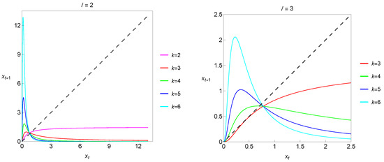
Figure 1.
Maps corresponding to different combinations of exponents l and k.
Throughout our entire study, we are going to fix . In this section, we consider and study the dynamics of the system
depending on the parameters and B. There is no particular reason for choosing and . If choosing other values, such as the also quite commonly used set of exponent values and , the model would have similar qualitative behavior and illustrative features of the dynamics. For the family of Hassell-type population models, there is considerable freedom to choose different combinations of the exponents l and k.
In order to provide a vision of certain global noticeable qualitative features of the dynamics of system (2), we display in Figure 2 a bifurcation diagram of vs. B, with and keeping . For all of the studied parameters, an increase in the carrying capacity, B, stabilizes the dynamics, although for large values of B, the population disappears due to the entry into the scenario of extinction (through a saddle-node bifurcation, as we will see in more detail in the next section).
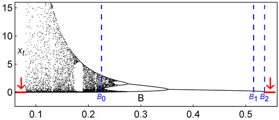
Figure 2.
Long-term behavior of the Hassell model (2): Bifurcation diagram of vs. B (the arrows indicate extinction scenarios). In this situation, and . The particular values of the carrying capacity depicted, , and , correspond to the iterated maps shown below in Figure 3 and to the iterated map shown in Figure 4.
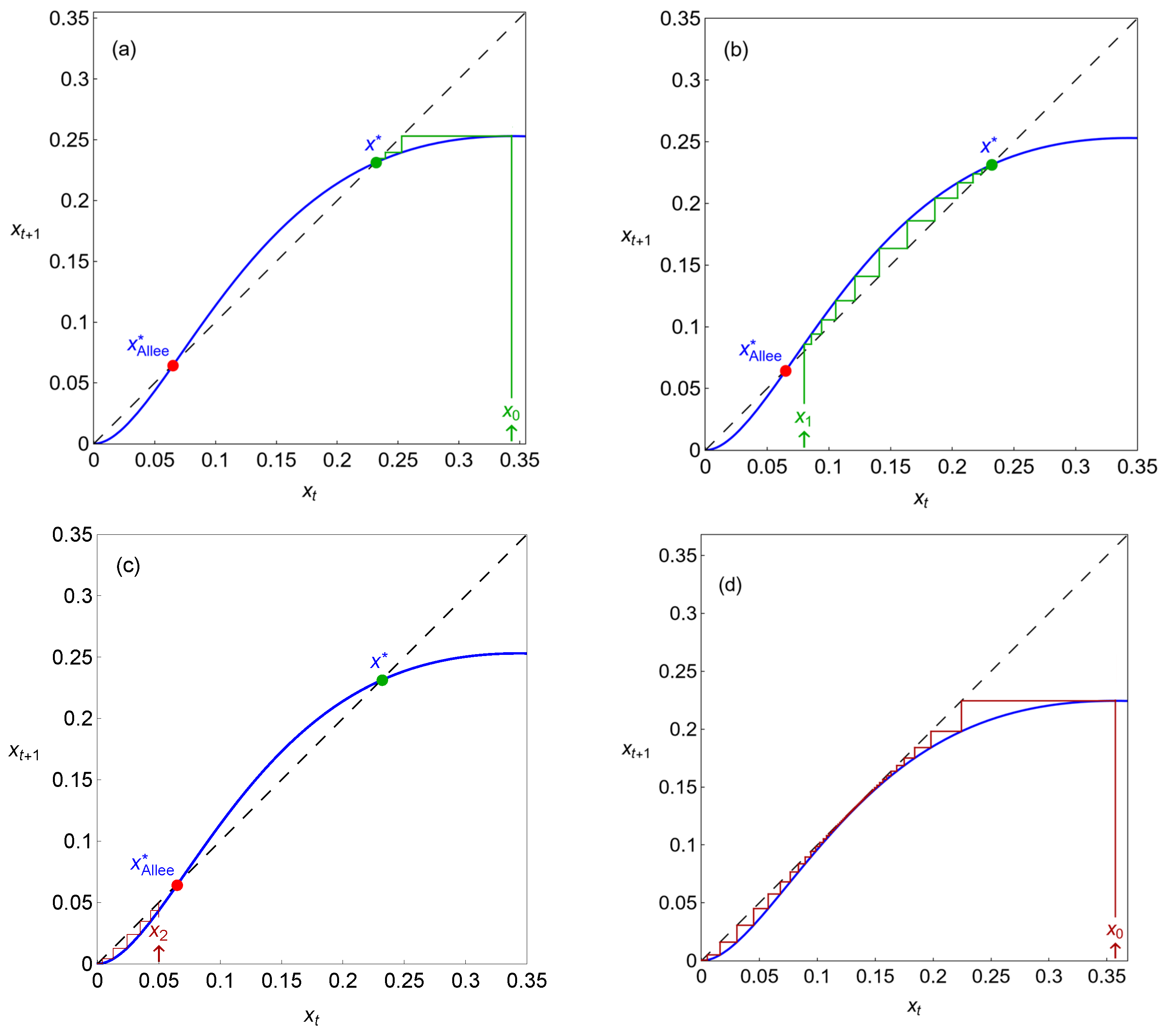
In Figure 3, we present maps showing the possible equilibrium points and iterations of the dynamical variable for different initial conditions. As illustrated in this figure, system (2) has the trivial equilibrium , which is stable for any parameter values. Along with , model (2) can possess two more real equilibria, and , such that (as presented in Figure 3a–c). The equilibrium is always unstable, and the stability of depends on the parameter values. A case where is stable is represented in Figure 3a–c, where the cobweb plots for system (2), with and , are exhibited. The Allee effect usually corresponds to the existence of a threshold population density. If the population size is less than this threshold, then the population is extinct; otherwise, the population exists in several regimes. In system (2), the role of this Allee threshold is played by the unstable equilibrium . Indeed, if , that is, if the initial condition is less than , then the solution vanishes, representing the population’s extinction (see the red iterations in Figure 3c). If , then the solution tends towards the stable equilibrium (see the green iterations in Figure 3a,b). The map of Figure 3d shows an extinction scenario which occurs after a saddle-node bifurcation point, where the stable and unstable equilibria merge and disappear (the iterations stay in a bottleneck region for a considerable time, causing delayed transitions, but always end up escaping to , as we will see in the next section).
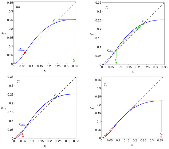
Figure 3.
Different maps showing the possible equilibrium points and cobweb iterations of the dynamical variable , with . The green lines represent survival iterations and the red lines represent extinction iterations. In (a–c), ; in (d), (particular values of the carrying capacity, represented in Figure 2, within the periodic regime).
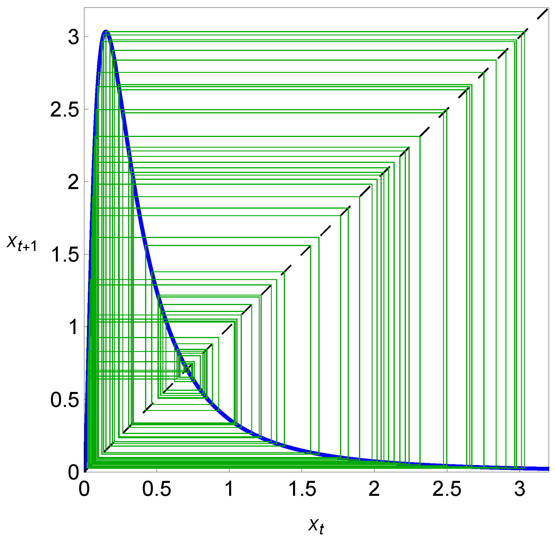
A case where is unstable is presented in Figure 4, where a cobweb plot for system (2), with and , is shown. In this case, as reported in Figure 4, the solution tends to the non-equilibrium regime (the cycle or chaotic attractor). In this chaotic regime, the cobweb plot is globally filled as a result of successive iterations. After the previous considerations, we easily understand that in system (2), the Allee threshold plays the role of a tipping point that separates two different dynamical regimes—extinction and persistence—under variations in the initial value of the population size.
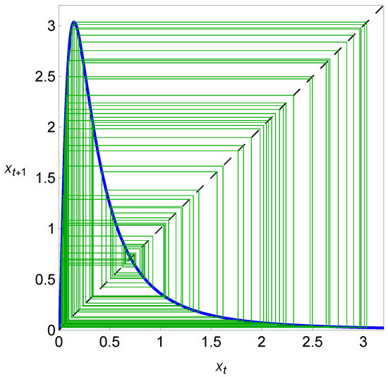
Figure 4.
A map depicting a cobweb plot with iterations of the dynamical variable with and (particular value of the carrying capacity, represented in Figure 2, within the chaotic region). In this chaotic regime, and as a result of successive iterations, the cobweb plot is globally filled, as illustrated by green lines.
In the study of dynamical systems, particularly one-dimensional maps, entropy and Lyapunov exponents are powerful tools for identifying and characterizing chaotic regimes.
Lyapunov exponents quantify the rate of separation of infinitesimally close trajectories in phase space. They measure how quickly nearby points diverge, or converge, as the system evolves, providing a quantitative measure of the system’s sensitivity to the initial conditions. In the study of chaotic dynamical systems, the computation of the Lyapunov exponents is critical in the sense that a positive Lyapunov exponent is a strong indicator of chaos. It signifies that small differences in the initial conditions grow exponentially, leading to unpredictable behavior. In particular, for an one-dimensional map like (2), if the only Lyapunov exponent that exists is positive, the system is considered chaotic.
As far as entropy is concerned, in general terms, it measures the rate of the production of information or the degree of unpredictability of the system. It quantifies the average rate at which new information is generated as the system evolves. It is also a strong indicator of chaos in the sense that a positive entropy value indicates that the system is producing information, which is a characteristic of chaotic behavior. Higher entropy values generally correspond to more complex and unpredictable chaotic regimes (see [19] and the references therein).
In short, the Lyapunov exponents provide a measure of the rate of divergence, while entropy provides a measure of the rate of information production. Together, they offer a more complete picture of the system’s dynamics. Both the Lyapunov exponents and entropy provide numerical values that can be used to precisely identify the onset and strength of chaotic behavior. By analyzing how the Lyapunov exponents and entropy change, as the system parameters are varied, we can distinguish between different types of chaotic regimes. In essence, the Lyapunov exponents and entropy provide crucial quantitative tools for detecting and characterizing the complex and unpredictable behavior associated with chaos (particularly in one-dimensional maps).
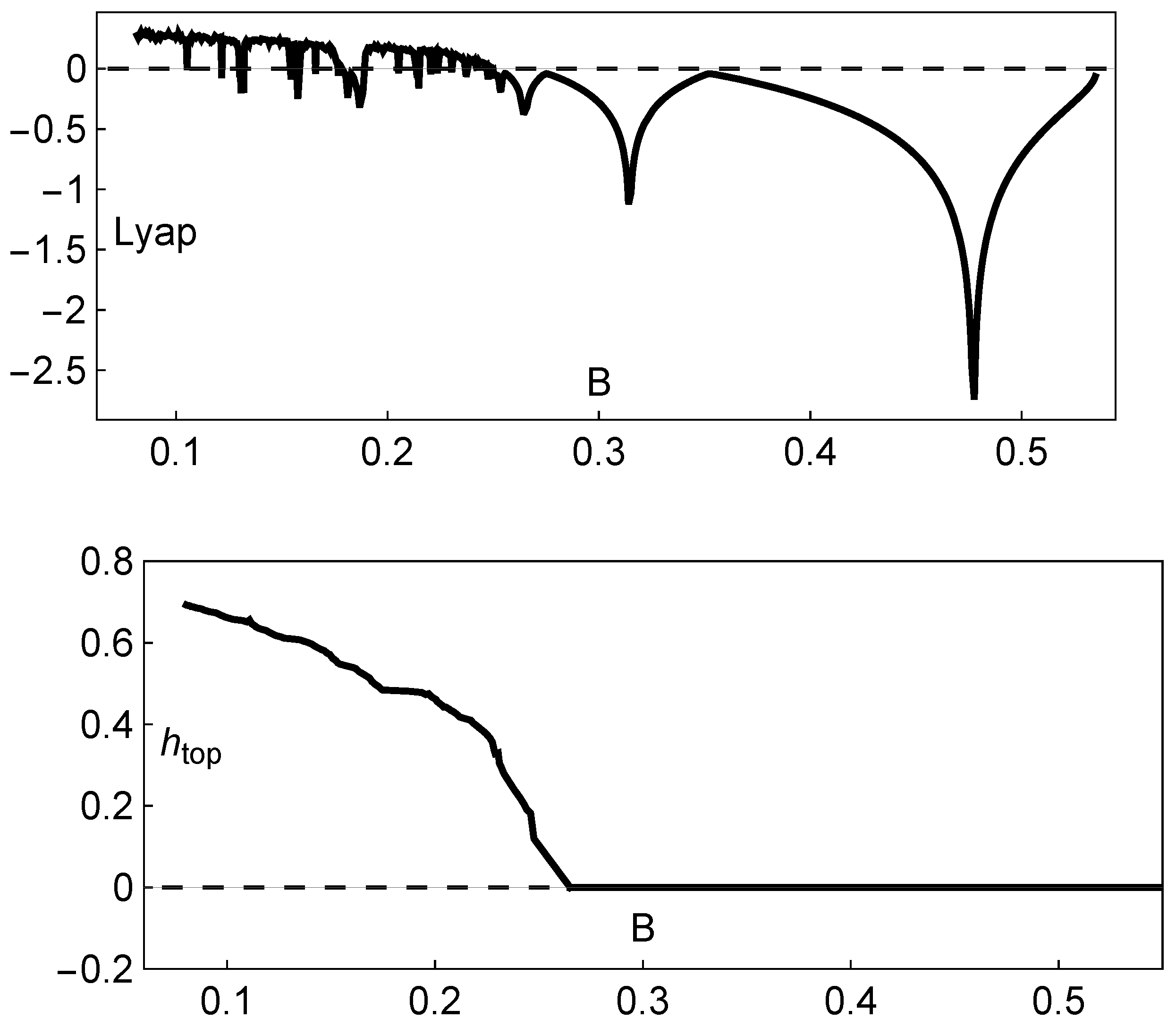
In agreement with the bifurcation diagram represented in Figure 2, the Lyapunov exponent is positive in the chaotic regime and negative in periodic regimes. In this way, the actual existence of chaos is numerically recognized when the Lyapunov exponent is positive (see the variation in the Lyapunov exponent shown in the upper panel in Figure 5).

Figure 5.
Dynamical features of the Hassell model (2). Upper panel: variation in the Lyapunov exponent with B; lower panel: variation in the topological entropy with B. In both situations, , and .
After numerical recognition of the existence of chaos, using the maximal Lyapunov exponent, it is significant to complement this analysis with the computation of the topological entropy—an important numerical invariant associated with the unimodal maps given by system (2). These maps on the interval, with two monotonic subintervals and one turning point, can benefit from the application of symbolic dynamics theory, mapping an interval into itself. In the context of symbolic dynamics theory, following the work carried out in [20] using Markov partitions closely, we compute an accurate estimate of the topological entropy as a measure of the amount of chaos. A positive value for the topological entropy is a sign of chaotic behavior (see the variation in the topological entropy depicted in the lower panel in Figure 5). The field of symbolic dynamics evolved as a tool for analyzing general dynamical systems by taking the state space and considering its partition into a finite number of regions, each of which is labeled with a given symbol. We obtain a symbolic trajectory by writing down the sequence of symbols corresponding to the successive partition elements visited by a point following some trajectory in the phase space. In this context, given a unimodal map f and an interval I subdivided into the sets , and , the function f is monotonically increasing for and monotonically decreasing for . The left and right subintervals are labeled with the letters L and R, respectively, and the set is denoted by C. The symbolic sequence starting from plays an important role in the symbolic dynamics of one-dimensional maps, and it is called a kneading sequence. As fully explained and exemplified in [20], the topological entropy of a unimodal interval map f, denoted by , is established as
where is the spectral radius, given by the characteristic polynomial, of the associated transition matrix . Studying the kneading sequences allows us to identify symbolic periodic orbits.
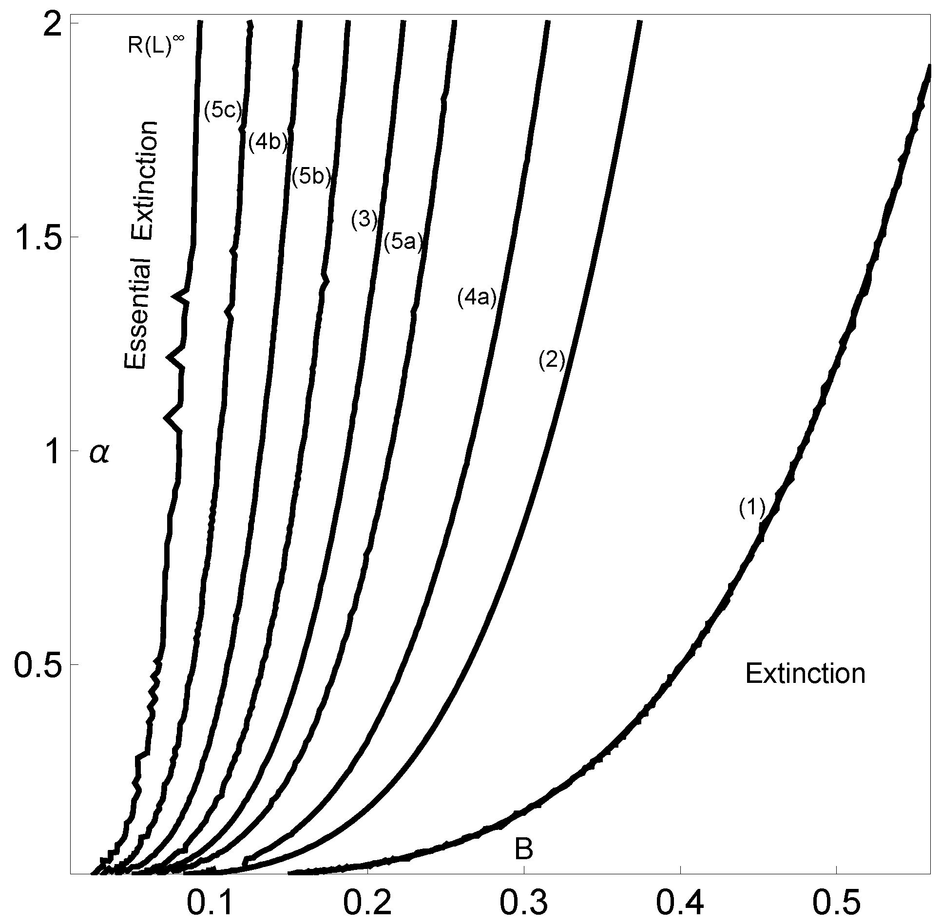
Now, using this methodology and in order to characterize the parameter space, we are going to compute the topological entropy while varying both B and . In Figure 6, nuclear periods of the symbolic dynamics (with ) are identified for decreasing values of entropy: period five (5c)-, period four (4b)-, period five (5b)-, period three (3)-, period five (5a)-, period four (4a)-, period two (2)- and period one (1)-C. Each curve depicted in this figure is isentropic. This means that each pair (B,) of the same curve corresponds to a map that produces the same kneading sequence, which is in turn associated with a particular value of the topological entropy. Different kneading sequences correspond to logistic-type iterated maps with different levels of complexity reflected in the different values for the topological entropy. The next table gives us information about the corresponding nuclear kneading sequences, studied in terms of their characteristic polynomials and topological entropy, that occur precisely for the regions reported in Figure 6. The codimension-two diagram in Figure 6 shows how the system’s dynamics change when the two control parameters vary.
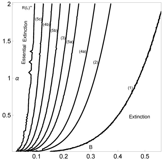
Figure 6.
Periods (in solid black lines) of the dynamics in the -parameter space using and . We also indicate the regions with asymptotic extinctions given by two scenarios: extinction and essential extinction. The periods found correspond to the kneading sequences given by the symbolic dynamics. These periods are indicated close to each corresponding line. The kneading sequences (with an increasing B) are as follows: period five (5c)-, period four (4b)-, period five (5b)-, period three (3)-, period five (5a)-, period four (4a)-, period two (2)- and period one (1)-C.
As a result of the analysis of the logistic-type iterated maps given by system (2) mentioned, the variation in both the topological entropy and the Lyapunov exponent is in agreement with the corresponding bifurcation diagram (Figure 2). According to the theory and using simple graphical terminology, the variation in the topological entropy follows the shape of the variation in the positive values for the Lyapunov exponent (for instance, see Figure 12 on page 633 in [21]). As we can observe, the dynamics of the system associated with positive topological entropy highlight the corresponding region of the parameter space where chaos occurs. The dynamics are particularly rich for a high amplitude of variation in the intrinsic growth rate , as can be observed in Figure 6. For low values of B, and in general independently of the value of , the system experiences an essential extinction scenario corresponding to a symbolic full shift. For pairs of parameter values within this particular region of the -parameter space, the iterate of the map’s critical point, after its first (and unique) iteration to the right, takes a value below the Allee threshold’s value, and as a consequence, the remaining iterates will forever tend to the left. At the full shift , the topological entropy has its maximum value. A further increase in B diminishes the complexity as the system undergoes inverse period-doubling bifurcations. The 3D plot of the Lyapunov exponent in Figure 7, along the -parameter region, complements some of this previous dynamical information.
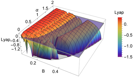
Figure 7.
A 3D plot of the Lyapunov exponent in the studied -parameter space (the horizontal plane separates the positive and negative values of the Lyapunov exponent).
3. Delayed Extinction: Dynamics Near a Saddle-Node Bifurcation
In this section, we study in detail the extinction scenario that occurs as a result of the occurrence of a saddle-node bifurcation. We provide the main calculations in the general mathematical framework for determining the time to extinction for any unimodal map undergoing a saddle-node bifurcation, here illustrated using Hassell-type system (1) with and . More precisely, we analytically derive the inverse square-root scaling law arising near the saddle-node bifurcation by using complex variable techniques. An analogous approach was applied to studying the scaling properties for saddle-node bifurcations in a general one-dimensional quadratic map [22]. For the sake of clarity, we will summarize the calculations in the following lines.
For a discrete dynamical system, the evolution of an iterate can be represented by the formula
As pointed out in [22], the equation can also be viewed as a difference equation
Hence, defining gives
which can be read “as t changes by 1 unit, x changes by ”. In this section, we are going to consider the Hassell-type system in order to study the scaling properties for a saddle-node bifurcation, analyzing
Therefore, defining
we obtain , with
Equilibrium points occur when . Besides the trivial solution , we have the equilibrium points of solutions of ; that is,
which is a cubic equation of the form
Defining the constants,
We have the following general scenarios:
- For , that is, ( = the bifurcation value of the parameter), with , all of the equilibrium points are real and distinct from each other;
- For , that is, , a saddle-node bifurcation occurs;
- For , that is, , one equilibrium point is real, and the others are complex conjugates.
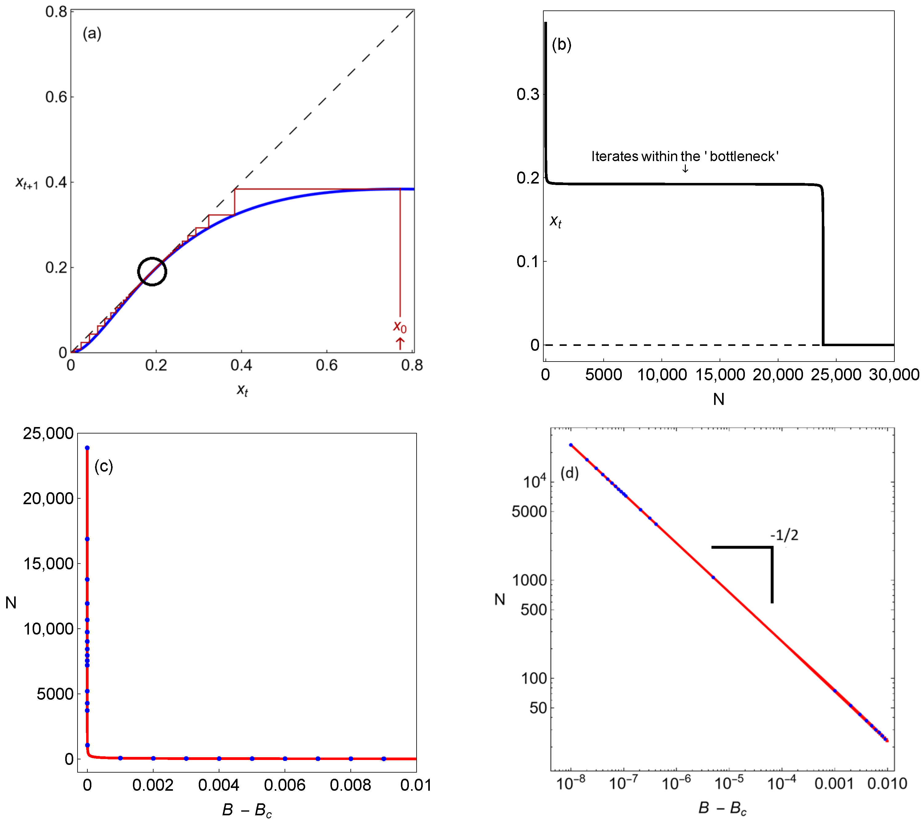
As can be seen in Figure 8a,b, when B is extremely close to (), many iterations of the map are required to pass through the bifurcation point. The reason for this local delay is the presence of a bottlenecking manifold (please see Figure 8a,b), which is also named a ghost [23] (represented by the black circle in Figure 8a). The scaling law measures the number of iterates required to pass through as a function of the difference in the parameter B from its bifurcation value (please see Figure 8c,d).
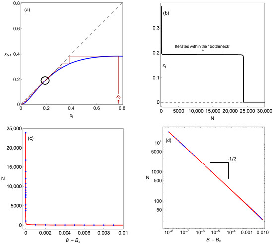
Figure 8.
Different dynamical features for system (3) associated with the extinction scenario: (a) We show the unimodal map after the saddle-node bifurcation. The unimodal map is below the diagonal, and the origin (which represents the population’s extinction) becomes globally stable; (b) the time before the population reaches the global trivial attractor suffers a delayed transition because of the action of the so-called ghost (the black circle in (a)). In (c), we show the dependence of the time before the species’ extinction, N, on the parametric distance to the bifurcation threshold. This time follows the inverse square-root scaling law: the solid line shows the analytical results using Equation (10), and, overlapping (blue circles), we show the numerical results; (d) the previous situation, now shown in log–linear scale.
The saddle-node bifurcation for the studied map takes place at when . Function (4) is analytic with respect to x in the neighborhood of . Sufficient conditions for such a bifurcation, when , are
and
Indeed,
In the following lines, we consider two new constants, a and b, such that and . As previously mentioned, the equilibrium points are the solutions of . Condition (5) allows us to apply the implicit function theorem and obtain that locally, the zeros for g close to are the points in the graph of an analytic function such that . Differentiating implicitly that , we obtain and .
For , we have . Since , we obtain . Therefore, we must proceed by computing the second derivative for the purpose of constructing the function h. From and since , we have . Using a Taylor expansion to construct , we obtain
With the purpose of having zeros in terms of B, we have to invert the previous expression. Except for , we obtain the following solutions:
For , we have the real solutions
with and . For , we obtain two complex solutions
also with .
As we already mentioned, our goal is to estimate the number of iterates needed to go from to in terms of B. Let us consider the equation presented at the beginning of this section, now expressed as
meaning that as t changes by one unit, x changes by Thus, the number of iterates required to go from to can be represented by
Let us consider expression (7) again and make . As a consequence of the application of the implicit theorem function, we notice that ; thus, gives way to . Therefore, in order to compute an approximate value for the sum (8), we consider the path integral
where , with , are the poles in the upper-half plane inside path . In our case, we only consider . Therefore, , with (see [24]). The computation of the residue is given by
Since , we can write
which leads to
Therefore, the number of iterates, N, required to pass through the bifurcation point for the Hassell-type model, given by , is approximated by
where
and , with , , , .
Delayed dynamical transitions correspond to long periods of time, which have the effect of prolonging the illusion of stability while increasing the extinction risk. The reason for this local delay in the population model’s dynamics is the presence of a bottlenecking manifold, resulting in a regime shift. In mathematical terms, this regime shift corresponds to a saddle-node bifurcation that eliminates the previously existing steady state when the system crosses a tipping point. This phenomenon, illustrated for our case in Figure 8a,b, is suggestively called a ghost due to the illusion of stability mentioned—the system behaves as if a stable point exists, but in fact, such a point no longer exists, with the population being at risk and doomed to extinction.
In the context of population dynamics, saddle-node bifurcations are common and truly critical, as they usually involve the transition from a survival scenario to the scenario of the extinction of a species. Not showing any signs of the upcoming decay for many generations, delayed dynamical transitions act silently in the ecosystem, making populations more vulnerable to catastrophes (please see the number of iterates within the bottleneck in the time series in Figure 8b). This represents a significant challenge for biological conservation and ecological management efforts because when this phenomenon is detected, it is often too late to avoid, or prevent, a sudden collapse. Understanding these delays is crucial for predicting tipping points and implementing timely interventions in threatened populations. A classical example of such behavior is the extinction debt resulting from habitat destruction (please see [25] and the references therein).
In Figure 8c,d, the number of iterates until the fixed point is reached is displayed as the intensity of the carrying capacity parameter grows above the limit point bifurcation. We exhibit the times to extinction obtained numerically using Equation (3) (represented by blue dots in Figure 8c,d) and analytically (represented by the solid line in Figure 8c,d) as described above. Note that the analytical results are in perfect agreement with the numerical ones. The number of iterates follows the inverse square-root scaling law, illustrated using the log–linear scale in Figure 8d.
4. Conclusions
Investigation of Allee effects in population ecology is a current subject of research. Field studies have shown the importance of population densities in the overall population dynamics under different ecological interactions. The study of Allee effects in complex ecosystems has been also carried out by investigating one-dimensional discrete models in the context of population dynamics.
This work bridges deterministic chaos and ecological collapse—by linking chaos, bistability and extinction mechanisms, it enhances our ability to predict and potentially mitigate catastrophic ecological transitions. This combination of mathematical approaches makes this study distinct in its contribution to both theoretical ecology and dynamical systems theory.
The analysis of the Allee effect within one-dimensional systems, while seemingly abstract, provides valuable insights that directly translate into real-world conservation efforts. In one-dimensional systems (e.g., along linear habitats like riverbanks, coastlines or mountain ridges), the dispersal is constrained, making them particularly susceptible to Allee effects. For example, if a population segment in a one-dimensional system falls below the Allee threshold, recolonization from other segments might be slow or ineffective. Studying these systems emphasizes the critical role of habitat connectivity. One-dimensional models help predict how invasive species spread along linear habitats. Understanding the Allee effect can reveal critical population thresholds that must be exceeded for successful invasion. When reintroducing endangered species, it is crucial to release enough individuals to overcome the Allee effect. Studies in one-dimensional systems help determine these critical thresholds, ensuring that reintroduction efforts are successful. Similarly, when augmenting existing populations, understanding the Allee effect helps conservationists determine the optimal number of individuals to add and where to release them. As far as the prioritization of conservation efforts is concerned, one-dimensional models demonstrate how habitat fragmentation can exacerbate the Allee effect, leading to rapid population declines. This highlights the need to prioritize conservation efforts in areas with fragmented linear habitats.
In essence, the study of the Allee effect in one-dimensional systems provides a framework for understanding how spatial constraints influence population dynamics. This knowledge translates into practical conservation strategies that focus on maintaining habitat connectivity, managing invasive species and ensuring the success of population reintroduction and augmentation efforts.
In the present article, we have studied one-dimensional Hassell-type maps describing single-species dynamics under an Allee effect. We have focused on the chaotic dynamics governing species survival. We studied the Lyapunov exponent, and using the theory of symbolic dynamics, we computed the topological entropy and codimension-two bifurcation diagrams by identifying the periods of the orbits. We have found that the appearance of transient chaos corresponds to the maximum topological entropy, with the symbolic dynamics , where a full shift takes place and the population becomes asymptotically extinct. Global noticeable qualitative features of the dynamics are present for wide variations in the parameters B and .
Finally, we have also investigated the delayed extinction transients due to saddle-node bifurcations. The analytically derived inverse square-root scaling law, via a complex analysis, offers a new perspective on how populations approach extinction through saddle-node bifurcations and allows us to compute the precise time to extinction. The analytical results are in complete agreement with the numerical results.
Author Contributions
Conceptualization: J.D., C.J. and N.M. Methodology: J.D. Software: N.M. Validation: J.D., C.J. and N.M. Formal analysis: J.D. Investigation: J.D., C.J. and N.M. Resources: J.D. and C.J. Data curation: J.D. Writing—original draft preparation: J.D. Writing—review and editing: J.D., C.J. and N.M. Visualization: J.D. Supervision: N.M. Project administration: N.M. Funding acquisition: J.D., C.J. and N.M. All authors have read and agreed to the published version of the manuscript.
Funding
Thisresearch was funded by the Portuguese Foundation for Science and Technology within the projects UIBD/04106/2025 (CIDMA) (C.J.) and UIBD/MAT/04459/2020 (J.D. and N.M.).
Data Availability Statement
Not applied to this research work.
Acknowledgments
The authors acknowledge the administrative and technical support provided by the research centers Centro de Análise Matemática, Geometria e Sistemas Dinâmicos (CAMGSD, IST) and Center for Research and Development in Mathematics and Applications (CIDMA, UA).
Conflicts of Interest
The authors declare no conflicts of interest. The funders had no role in the design of this study; in the collection, analyses or interpretation of the data; in the writing of the manuscript; or in the decision to publish the results.
References
- May, R.M. Simple Mathematical models with very complicated dynamics. Nature 1976, 261, 459–467. [Google Scholar] [CrossRef] [PubMed]
- Hastings, A. Population Biology: Concepts and Models; Springer: New York, NY, USA, 1997. [Google Scholar]
- Zhang, L.; Liu, J.; Banerjee, M. Hopf and steady state bifurcation analysis in a ratio-dependent predator-prey model. Commun. Nonlinear Sci. Numer. Simul. 2017, 44, 52–73. [Google Scholar] [CrossRef]
- Gladwell, M. The tipping Point: How Little Things Can Make a Big Difference; Little Brown: Boston, MA, USA, 2000. [Google Scholar]
- Allee, W.C. The Social Life of Animals; William Heinemann: London, UK, 1938. [Google Scholar]
- Allee, W.C.; Emerson, A.E.; Park, O.; Park, T.; Schmidt, K.P. Principles of Animal Ecology; Saunders: Philadelphia, PA, USA, 1949. [Google Scholar]
- Cánovas, J.S.; Muñoz-Guillermo, M. On the dynamics of a linear-hyperbolic population model with Allee effect and almost sure extinction. Appl. Math. Comput. 2025, 486, 129005. [Google Scholar] [CrossRef]
- Gao, M.; Chen, L.; Chen, F. Dynamical analysis of a discrete two-patch model with the Allee effect and nonlinear dispersal. Math. Biosci. Eng. 2024, 21, 5499–5520. [Google Scholar] [CrossRef] [PubMed]
- Cánovas, J.S.; Muñoz-Guillermo, M. On a population model with density dependence and Allee effect. Theory Biosci. 2023, 142, 423–441. [Google Scholar] [CrossRef] [PubMed]
- Zhou, Q.; Chen, Y.; Chen, S.; Chen, F. Dynamic analysis of a discrete amensalism model with Allee effect. J. Appl. Anal. Comput. 2023, 13, 2416–2432. [Google Scholar] [CrossRef] [PubMed]
- Sen, D.; Sinha, S. Enhancement of extreme events through the Allee effect and its mitigation through noise in a three species system. Sci. Rep. 2021, 11, 20913. [Google Scholar] [CrossRef] [PubMed]
- Elaydi, S.; Kwessi, E.; Livadiotis, G. Hierarchial competition models with the Allee effect III: Multispecies. J. Biol. Dyn. 2018, 12, 271–287. [Google Scholar] [CrossRef] [PubMed]
- Hassell, M. Density Dependence in Single-Species Population. J. Anim. Ecol. 1975, 44, 283–295. [Google Scholar] [CrossRef]
- Hassell, M.P.; Lawton, J.H.; May, R.M. Patterns of Dynamical Behaviour in Single-Species Populations. J. Anim. 1976, 45, 471–486. [Google Scholar] [CrossRef]
- Geritz, S.A.H.; Kisdi, E. On the mechanistic underpinning of discrete-time population models with complex dynamics. J. Theor. Biol. 2004, 228, 261–269. [Google Scholar] [CrossRef] [PubMed]
- Bascompte, J.; Solé, R.V. Spatially Induced Bifurcations in Single-Species Population Dynamics. J. Anim. Ecol. 1994, 63, 256–264. [Google Scholar] [CrossRef]
- Bashkirtseva, I. Crisis, noise, and tipping in the Hassell population model. Chaos 2018, 28, 033603. [Google Scholar] [CrossRef] [PubMed]
- Bashkirtseva, I.; Ryashko, L.; Spagnolo, B. Combined impacts of the Allee effect, delay and stochasticity: Persistence analysis. Commun. Nonlinear Sci. Numer. Simul. 2020, 84, 105148. [Google Scholar] [CrossRef]
- Cánovas, J.S.; Muñoz-Guillermo, M. On the complexity of economic dynamics: An approach through topological entropy. Chaos, Solitons Fractals 2017, 103, 163–175. [Google Scholar] [CrossRef]
- Duarte, J.; Januário, C.; Rodrigues, C.; Sardanyés, J. Topological complexity and predictability in the dynamics of a tumor growth model with Shilnikov’s chaos. Int. J. Bifurc. Chaos 2013, 23, 1350124. [Google Scholar] [CrossRef]
- Eckmann, J.P.; Ruelle, D. Ergodic theory of chaos and strange attractors. Rev. Mod. Phys. 1985, 57, 617–656. [Google Scholar] [CrossRef]
- Duarte, J.; Januário, C.; Martins, N.; Sardanyés, J. Scaling law in saddle-node bifurcations for one-dimensional maps: A complex variable approach. Nonlinear Dyn. 2012, 67, 541–547. [Google Scholar] [CrossRef]
- Strogatz, S.H. Nonlinear Dynamics and Chaos with Applications to Physics, Biology, Chemistry, and Engineering; Westview Press: Boulder, CO, USA, 2000. [Google Scholar]
- Fontich, E.; Sardanyés, J. General scaling law in the saddle-node bifurcation: A complex phase space study. J. Phys. A Math. Theor. 2008, 41, 015102-1. [Google Scholar] [CrossRef]
- Morozov, A.Y.; Almutairi, D.; Petrovskii, S.V.; Hastings, A. Regime shifts, extinctions and long transients in models of population dynamics with density-dependent dispersal. Biol. Conserv. 2024, 290, 110419. [Google Scholar] [CrossRef]


Disclaimer/Publisher’s Note: The statements, opinions and data contained in all publications are solely those of the individual author(s) and contributor(s) and not of MDPI and/or the editor(s). MDPI and/or the editor(s) disclaim responsibility for any injury to people or property resulting from any ideas, methods, instructions or products referred to in the content. |
© 2025 by the authors. Licensee MDPI, Basel, Switzerland. This article is an open access article distributed under the terms and conditions of the Creative Commons Attribution (CC BY) license (https://creativecommons.org/licenses/by/4.0/).