Abstract
This study aims to reveal the network connectedness between the volatilities of Emerging and Growth-Leading Economies (EAGLEs) stock exchanges with the frequency-based TVP-VAR connectedness approach. Connectedness results were obtained in short (1–5 days) and long (5-inf) period frequencies among the volatilities obtained with the Garman–Klass volatility estimator. According to the dynamic TCI results, connectivity peaked during the COVID-19 and Russia–Ukraine War periods. BVSP is the most dominant transmitter of the network and spreads the most effect to the emerging markets. As a result of the pairwise metrics, SSE has the lowest values and is positioned as a relatively independent market in the network. In particular, SSE has almost no connection with BIST in the short term, while it has a more significant effect on BIST in the long term. Moreover, the connectedness metrics show that MOEX is in a neutral position in the network and is largely affected by its internal dynamics.
Keywords:
EAGLEs countries; frequency connectedness; pairwise connectedness; portfolio diversification; TVP-VAR MSC:
37A60; 70-08; 70-10; 76-10; 74P10
1. Introduction
Global financial markets have become increasingly interconnected over the past few decades, driven by financial liberalization, technological advancements, and economic integration [1,2,3]. While this interconnectedness fosters economic development, it simultaneously amplifies systemic risks, particularly during crises. Key issues such as volatility spillovers, asymmetric connectedness, and contagion effects have significant implications for risk transmission, portfolio diversification strategies, and financial stability [4,5]. These challenges are particularly pronounced in the context of emerging economies, such as the EAGLE countries; namely, Brazil, China, India, Indonesia, Korea, Mexico, and Turkey, which play a pivotal role in the global financial network. Notably, EAGLE economies are projected to account for 64% of the anticipated global GDP growth, underscoring their critical influence on future economic trends [6,7,8]. However, their deeper integration into global markets has intensified return and volatility spillovers, especially during periods of global crises [9]. Geopolitical events, such as the U.S.–China trade war and the Russo–Ukrainian armed conflict, have further exacerbated these spillovers, heightening market uncertainty and systemic risks in interconnected economies [10,11].
Emerging markets exhibit distinct patterns of return and volatility spillovers, reflecting their deep integration into the global financial system and their exposure to both regional proximity and global dynamics. Indonesia’s historically strong financial ties with Singapore and Thailand underscore the critical role of regional stability in mitigating systemic risks, as instant shock transmission exposes vulnerabilities in interconnected markets [12]. Similarly, China’s pivotal role in ASEAN volatility demonstrates how policies like the 2015 RMB peg adjustment triggered significant spillovers across regional stock and currency markets, particularly affecting Indonesia and Malaysia [13,14]. South Korea, as a key net transmitter of volatility during crises, highlights its systemic importance within the Asia-Pacific financial network [15]. In Latin America, the Mexican Stock Exchange (IPC) maintains a strong long-term equilibrium relationship with the global capital market, although high-volatility periods, such as the 2008 financial meltdown, amplify systemic risks [16]. The IPC’s stable interdependency structure positions it as a critical node linking Latin America to U.S. markets [17,18].
Meanwhile, quantile-connectedness analysis reveals pronounced bidirectional spillovers between the VIX and global stock returns during high-volatility periods, underscoring the challenges of managing systemic risks in increasingly interconnected markets [19]. Systemic shocks, such as those stemming from the COVID-19 pandemic, further expose vulnerabilities in emerging markets, with South Korea transmitting return spillovers and China, India, and Indonesia acting as key receivers, particularly during global crises [7]. China’s dominant position as a net transmitter of return spillovers reinforces its systemic importance in the Asia-Pacific and the broader global financial landscape [20,21]. India and Brazil play dual roles as both recipients and transmitters of volatility, with India acting as a vital link between regional and global financial systems. Meanwhile, Mexico’s deeper integration into global markets aligns its risks closely with global trends, diminishing diversification benefits during periods of heightened volatility [22].
The recent literature offers strong evidence of evolving interdependence among emerging markets, particularly across BRICS and EAGLE member constituents. Hong Vo and Dang [23] apply a quantile frequency connectedness approach and highlight that long-term spillovers dominate short-term ones across BRICS equity markets, particularly under geopolitical risk. Similarly, Agyei et al. [24] use the Baruník and Křehlík [25] time-frequency decomposition to analyze BRIC–G7 market linkages, revealing short-term contagion channels that intensified during global crises. Focusing on pre-pandemic conditions, Shi [26] employs a generalized VAR spillover index and shows that short-term return spillovers are most pronounced among BRICS, especially from China and Russia, while Brazil’s role varies across time.
Spillover dynamics also featured prominently in studies of regional interactions. Khan et al. [27], using the Diebold and Yilmaz (DY) framework, examine Asian emerging stock markets and report significant return spillovers from China and India to countries such as Indonesia and Malaysia. Asafo-Adjei et al. [28] adopt a Kalman Filter-based wavelet approach to track systematic risk interdependence in 20 emerging markets, including Brazil, China, and India, and document sustained integration during periods of market turbulence.
Market-specific responses to global shocks have been explored using more targeted quantile-based frameworks. Anyikwa and Phiri [29] reveal that Brazil and India consistently acted as net transmitters of systemic shocks, while China remained a persistent net receiver during both the COVID-19 pandemic and the Russo–Ukrainian armed conflict. Recent analysis by Sayed and Charteris [30] also confirms that India and Brazil played pivotal roles in volatility transmission during COVID-19. Complementing this, Asafo-Adjei et al. [28] emphasize that market resilience differs substantially by country, with Brazil and China showing a relatively higher susceptibility to systemic risks.
From a structural segmentation standpoint, Sayed and Charteris [30] find that, after controlling for the effects of global influences, India emerged as the most integrated BRICS stock market, while Brazil and China remained the most segmented. These findings are supported by Gurdgiev and O’Riordan [31], who use wavelet coherence and phase analysis to show that Brazil’s integration with the U.S. intensified post-GFC, while China’s 2015 stock market crash had widespread contagion effects on U.S., European, and Japanese markets. Batondo and Uwilingiye [32] provide further support, documenting time-varying co-movement between BRICS and the U.S. market, with Brazil being most vulnerable to external trade-related shocks.
Asymmetric volatility spillovers are also a recurring theme in financial markets, with negative shocks often playing a dominant role in propagating systemic risks. Mensi et al. [33] examine the asymmetric volatility connectedness between Bitcoin and major precious metals, finding that negative shocks dominate spillover effects. Similarly, Baruník et al. [34] observe comparable patterns in the foreign exchange market, where adverse shocks are critical in transmitting risks across currencies.
Moreover, recent evidence from the Asia-Pacific currency markets underscores pronounced asymmetries in volatility connectedness during high-stress periods, such as financial crises and geopolitical tensions. Negative shocks were found to propagate more strongly across currencies during the COVID-19 pandemic and the U.S.–China trade war, further destabilizing market stability [11]. In oil markets, Liu et al. [10] identify that negative spillovers from WTI and Brent crude oil futures play a dominant role in transmitting volatility to emerging markets, exacerbating systemic risks during periods of economic uncertainty.
Similarly, cryptocurrency and energy markets exhibit significant volatility asymmetry, with spillovers predominantly flowing from energy markets to cryptocurrencies. These dynamics are further amplified by factors such as electricity consumption and geopolitical uncertainties, particularly during crises like the COVID-19 pandemic [35]. Pandemics such as COVID-19 have significantly heightened these dynamics, with elevated volatility spillovers diminishing the traditional safe-haven roles of assets like Bitcoin, gold, and oil, as regional stock indices experience increased contagion during crises [36].
Furthermore, the renewable energy sector also demonstrates asymmetric volatility spillovers, with fuel cell stocks acting as net transmitters and wind energy stocks as net receivers, reflecting their distinct roles in systemic risk propagation during periods of stress [37]. Similarly, Yang [38] investigates the spillover structure between electricity and carbon markets in Europe and finds that idiosyncratic information transmission is asymmetrically distributed, with electricity markets acting as dominant shock transmitters, particularly during regulatory shifts and peak-load conditions. These findings underscore the broader significance of asymmetry in financial markets, providing a critical foundation for exploring such dynamics within EAGLE economies. Shahzad et al. [39] reveal that during the COVID-19 pandemic, bad volatility spillovers overwhelmingly dominated good volatility spillovers across Chinese sectors, particularly in highly interconnected industries such as consumer staples and energy.
Within the context of EAGLE countries, volatility spillovers tend to escalate throughout financial crises, with Turkey, Brazil, India, and Indonesia frequently acting as net receivers of volatility, while China, Russia, and Mexico emerge as net transmitters [6,9]. These spillovers, as portrayed by M. Umer et al. [40] through multivariate GARCH models, are highly time-sensitive, often peaking during post-crisis recovery phases. A time-frequency domain analysis of Asia-Pacific currencies further reveals that short-term volatility spillovers dominate during crises, whereas long-term spillovers are more prominent in periods of relative market stability [41]. This dynamic is also mirrored in Brazil, where the total connectivity of financial and non-financial sector indices averaged 66% over eight years, with significant peaks during political and economic crises [21]. Similarly, Liu et al. [10] highlight that in oil markets, short-term spillovers are particularly pronounced, emphasizing their critical implications for energy-dependent EAGLE economies. Beyond temporal volatility, governance quality and institutional factors are pivotal in shaping spillover dynamics. Arif and Rawat [42] and Khan et al. [43] highlight that enhancing governance and fostering regional cooperation can strengthen market resilience against external shocks. Moreover, interconnectedness metrics provide valuable early warning tools, enabling policymakers to address systemic risks proactively [44]. EAGLE economies’ deep interconnectedness with developed markets also plays a significant role in influencing volatility patterns [40,45]. Recent analyses of ETF market dynamics suggest that alternative ETFs transmit fewer systemic risks and may act as stabilizers during crises, offering a particularly valuable strategy for economies integrating into global financial markets.
Despite the breadth of evidence on spillover dynamics, several patterns emerge across the reviewed studies. First, volatility and return spillovers in emerging markets are not static at all but rather evolve in response to global uncertainty, geopolitical shocks, and structural integration processes. China, India, and Brazil repeatedly appear as central nodes, either as net transmitters or highly responsive receivers, depending on market phases and the nature of the shock. Second, while regional segmentation persists, long-run co-movements, especially those tied to energy markets and U.S. financial developments, intensify during crises. This highlights both contagion risks and limits to potential benefits from diversification. Methodologically, the literature reflects growing consensus that static models are insufficient to fully capture the temporal heterogeneity, asymmetries, and nonlinearities embedded in emerging market dynamics. Still, relatively few studies offer bilateral, high-frequency, or directionally detailed insights across time and frequency, a gap that underscores the need for more integrated modeling frameworks.
In this context, the time-varying parameter vector autoregressive (TVP-VAR) model in the frequency domain provides a powerful methodological alternative. Unlike traditional DY models, which assume static relationships, or wavelet-based methods, which often lack bilateral directional metrics, the TVP-VAR framework jointly captures evolving pairwise connectedness and decomposes spillovers into short- and long-term components. Compared to QVAR models, which are well-suited for analyzing tail dependencies but limited in frequency resolution, the TVP-VAR approach offers a more granular view of interdependence. By enabling bilateral, dynamic, and frequency-specific analysis, it bridges the limitations of existing frameworks and contributes a high-resolution lens for mapping systemic risk in emerging economies.
Building on scarce prior research, such as M. Umer et al. [40] and Bozma et al. [6], which analyze volatility spillovers among EAGLE economies, this study takes a significant step forward by being both methodologically different and innovative in terms of the period analyzed. In addition, it reveals short- and long-term dynamics in the frequency domain. Earlier studies have largely focused on pre- and post-crisis volatility patterns within static frameworks, leaving evolving dynamics and interdependencies underexplored. To address this gap, short- and long-term dynamic connectivity results and related metrics are presented with TVP-VAR frequency connectedness analysis. In particular, the applied pairwise metrics and the obtained bilateral connectivity results are important contributions to this study. By employing the time-varying parameter VAR framework in the frequency domain, this paper provides directionally explicit, bilateral spillover measures that outperform traditional static and wavelet-based models in capturing evolving volatility dynamics. Moreover, by utilizing recent and comprehensive data over an extended timeframe, this study aligns its analysis with the realities of contemporary global financial integration. Ultimately, these methodological advancements enable a finer decomposition of contagion patterns among EAGLE economies, uncovering how systemic risk is transmitted and absorbed across different time horizons. As such, the study enhances the understanding of financial interconnections within the EAGLE network by identifying persistent transmitters, vulnerable receivers, and evolving bilateral ties, especially during crisis periods.
2. Materials and Methods
2.1. Dataset
This study utilizes a dataset comprising daily OHLC (Open, High, Low, Close) prices data for eight stock market indices representing economies classified under the EAGLE (i.e., Emerging and Growth-Leading Economies) framework. We aim to analyze the connectedness between the volatility series, which are estimated volatility values derived from the daily OHLC prices of the stock exchanges using the Garman–Klass method. In other words, our data are not directly observed volatility but volatility indicators calculated based on prices. These economies are identified based on their significant contributions to global economic growth projections. The dataset spans from 2 January 2019 to 14 November 2024, offering a comprehensive time series for examining volatility connectedness across these emerging markets. The stock market indices included in the analysis are Brazil’s BVSP (Bovespa Index), China’s SSE (Shanghai Stock Exchange), India’s BSE (Bombay Stock Exchange), Indonesia’s IDX (Jakarta Stock Exchange), South Korea’s KOSPI (Korea Composite Index), Mexico’s IPC (Índice de Precios y Cotizaciones), and Türkiye’s BIST (Borsa Istanbul Index), all of which were sourced from the Yahoo Finance database. To ensure complete data coverage for the given period, Russia’s MOEX (Moscow Exchange Index) data was obtained from Investing.com.
The purpose of choosing this period is to include the impact of global shocks that caused sudden and large fluctuations in financial markets, such as the COVID-19 pandemic and the Russia–Ukraine war, in the model. In order to reveal the impact of events such as the closure of the Russian Stock Exchange MOEX immediately after the Russo–Ukrainian War and its opening two weeks later, a special filtering was performed in the data pre-processing stage to eliminate inconsistencies arising from the holiday calendars of different country stock exchanges. The days when any country’s market was closed (no trading) were simultaneously removed from the data set of all countries. Thus, only the common trading days when all markets are open remained in the panel data set, and the data was fully synchronized. As a result of this method, there were no missing observations in the data set; therefore, no missing data estimation or similar intervention was required.
2.2. Garman–Klass Volatility Estimator
Intraday Opening-Highest-Lowest-Closing (OHLC) prices serve as a critical component in volatility estimation within technical analysis, providing a more comprehensive representation of price fluctuations in comparison to methods that rely solely on closing prices. By incorporating intraday price movements, OHLC-based volatility estimators capture market dynamics with greater precision, leading to more reliable measurements of asset price variability. Amongst these estimators, the Garman–Klass (GK) model is widely recognized for its ability to enhance volatility estimation accuracy. Unlike the conventional closing-to-closing (CC) volatility estimator, which only considers consecutive closing prices, the GK estimator leverages the full range of price movements within a trading period, incorporating the highest, lowest, and closing prices. This broader inclusion of market information renders the GK estimator significantly more efficient, improving its precision by a factor of approximately 7.4 compared to the CC estimator [46,47]. The GK estimator is formulated under the assumption that logarithmic asset prices follow a geometric Brownian motion with zero drift, ensuring a continuous price evolution without abrupt jumps at market opening. These underlying assumptions reinforce the estimator’s robustness by aligning the opening price with the previous session’s closing price, thereby improving the reliability of volatility calculations. The GK estimator formula is defined herein as follows:
Assuming zero drift ensures that the volatility estimate remains unaffected by underlying price trends, thereby isolating pure volatility dynamics. Additionally, the exclusion of opening spikes eliminates distortions introduced by external market factors, preserving the integrity of the estimated volatility. Given its superior efficiency, the GK estimator is widely favored in financial connectivity studies, particularly when historical intraday OHLC data are available, as it offers a more precise representation of market fluctuations in comparison to alternate volatility estimation methods.
Like other OHLC-based estimators, the volatility series obtained with the GK method are stationary at the level. Stationarity at the level is a necessary condition for the application of the TVP-VAR model. Another reason for using the GY approach is that the volatility series obtained from EWMA, CARR, and other GARCH-family models are not always stationary at the level. In addition, the Garman–Klass estimator was utilized in the papers of Diebold and Yilmaz [48] and Demirer et al. [49], which pioneered the volatility spillover and connectivity studies. For these reasons, the volatility estimator has been widely used in GY Diebold-Yilmaz-Connectedness related studies. First of all, since we cannot observe volatility directly (it is a latent variable), we have to use an estimator in every case, and each estimator we use will have certain assumptions and limitations. Although we accept that the Garman–Klass method may lead to some deviations in crisis periods, since the volatility of all markets examined in our study is calculated consistently with the same method, the effect of possible bias on the comparative results is limited. In particular, our volatility connectedness analysis focuses on the relative dynamics of volatility movements between markets rather than absolute volatility levels. Even if Garman–Klass underestimates absolute volatility in crisis periods, since the measurement is made with a similar approach for all markets, the relative increases and common movements in the relevant periods are largely captured. Therefore, the main results of our volatility spillover analysis (e.g., the findings of simultaneous increase in volatility and increased connectivity across all EAGLE markets during crisis periods) are valid.
Descriptive Assessment for Volatility Series
Figure 1 displays the evolution of OHLC-based GK volatility in stock exchanges from early 2019 to late 2024. The volatility levels in all markets, except MOEX, peaked during the COVID-19 pandemic, underscoring the significant market-wide impact of the crisis. While volatility generally declined in the post-pandemic period, a renewed upward trend is observed towards the end of 2024, potentially driven by uncertainty surrounding the U.S. elections. In contrast, MOEX exhibited its highest volatility levels during the onset of the Russo–Ukrainian armed conflict, emphasizing the sensitivity of financial markets to geopolitical occurrences. Market-specific dynamics further illustrate differences in volatility transmission wherein the Brazilian market demonstrates a remarkable ability to propagate volatility to other financial markets during periods of heightened fluctuations, while SSE maintains relatively lower volatility levels compared to its counterparts.
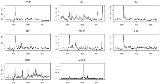
Figure 1.
Time Series Plots of Garman–Klass OHLC Volatility Series.
BSE plays a significant role in transmitting volatility to other Asian markets, whereas IDX stands out as an influential market in short-term volatility spillovers. The sharp increase in IDX’s volatility towards the end of 2024 suggests its susceptibility to global developments. Similarly, Mexico’s IPC has experienced a marked rise in volatility throughout 2024, reinforcing its role in both short-term and long-term financial interdependencies. The Turkish market, as represented by BIST, followed a relatively stable trajectory between 2021 and 2023, yet its exposure to regional events remains evident. Meanwhile, the Russian market exhibited fewer pronounced peaks in volatility than other markets, with its highest fluctuations largely attributed to geopolitical tensions. Overall, these observations reinforce the interconnected nature of global financial markets, particularly in times of economic and political uncertainty. The significant volatility surges witnessed during the COVID-19 pandemic highlight the systemic nature of market disruptions, while the renewed turbulence in late 2024 may reflect mounting global financial risks.
Table 1 presents the summary statistics with regard to volatility series. As expected, the average volatility values are positive for all stock markets. Since volatility is a non-negative measure by definition, this result is consistent with the nature of the data and the construction of the volatility estimator. The highest average volatility value is observed in BIST (0.209), while the lowest is observed in IDX (0.118). ERS test results are statistically significant and support the stationarity assumption of the series for further econometric approaches. At the same time, Ljung-Box test results portray that the series have autocorrelation both at the level (Q(20)) and squares (Q2(20)). Volatility variances are highest in MOEX (0.037), and lowest in SSE and IPC (0.002). This shows that MOEX is the most volatile, while SSE and IPC are more stable. The skewness values are positive and significant, indicating an asymmetric distribution in the volatility series. MOEX has the highest skewness (14.221), while BIST has the lowest (2.255). The extreme values are also significantly large, indicating that the series have heavy tails and deviations from the normal distribution. MOEX again has the highest value (313.575). The JB test values are significant for all series, confirming that the volatility series deviate from the normal distribution.

Table 1.
Descriptive Statistics of Volatility Series and Spearman Correlation Matrix.
MOEX stands out as the riskiest market in terms of volatility, having the highest variance (0.037), skewness (14,221), and excess kurtosis (313,575) values, demonstrating that high risk and extreme behaviors are frequent occurrences in this market, while BIST has the highest average volatility but exhibits lower skewness and extremes. This shows that Russia is seriously affected by international sanctions, energy market shocks, and geopolitical tensions. BIST, which has the highest value in terms of average volatility (0.209), offers both opportunity and risk for investors due to high volatility. Although the skewness and extreme values are relatively low, liquidity problems or local political uncertainties can affect this volatility. The Chinese and Mexican stock exchanges have the lowest variance (0.002). This indicates more stable market conditions and limited volatility.
Correlations indicate strong joint movements, especially based on regional connections or economic relations such as IDX-KOSPI. However, exchanges with weaker connections such as BIST and SSE indicate different macroeconomic dynamics. To be more specific: There is a strong and significant correlation between the South Korean stock exchange KOSPI and the Indonesian stock exchange IDX with a value of 0.524. This relationship may be due to economic connections and trade relations in the Asia-Pacific region. A moderate correlation is observed between the KOSPI and the Mexican stock exchange IPC with a correlation value of 0.455. This may indicate the effects of common sectors in global trade networks. There is a stronger than expected correlation between the Brazilian stock exchange BVSP and KOSPI with a value of 0.495. This may be due to international investor behavior in the technology sector. The correlation value between BIST and SSE is 0.017, and no statistically significant relationship is observed between the Turkish and Chinese stock exchanges. It is seen that these two markets have independent macroeconomic dynamics and that investor behaviors move in different directions. The same situation is observed between BIST and BSE stock exchanges with a value of 0.024. A weak relationship between Turkish and Indian stock exchanges can also be explained by geographical distance and different economic structures. A relatively low coefficient emerged between BIST and MOEX with a correlation value of 0.224. In other words, there is a statistically significant but weak relationship between Türkiye and Russia. Despite geographical proximity and cooperation in energy markets, the volatility dynamics appear to be quite different.
2.3. Frequency-Based Tvp-Var Volatility Connectedness
Baruník and Křehlík [25] expanded the financial connectedness framework initially developed by Diebold and Yilmaz [55,56,57] by introducing a frequency-based methodology that captures dynamic market relationships over different time horizons. The pioneering study of connectedness analysis, Diebold and Yilmaz [55], used a connectivity measure based on Cholesky decomposition for VAR model residuals. This orthogonalization method is sensitive to the order of variables and requires the assumption of structural constraints in the model, for example, a hierarchical order of influence among variables. Later, Diebold and Yilmaz [56] adopted the generalized VAR approach developed by Pesaran and Shin [58] in order to be insensitive to the order of variables; this method is based on the order-independent generalized prediction error variance decomposition (GFEVD).
Despite this advancement, both the Cholesky-based approach and the generalized approach use the assumption that the model parameters remain constant over time. When a dynamic structure is desired, VARs are usually estimated in different sub-periods with the rolling window technique, and the connectedness index is obtained over this rolling window. Using a sliding window, however, brings other problems: The window length needs to be determined arbitrarily, and this choice can seriously affect the results. For example, a narrow window selection can make the model parameters too volatile and overreact to shocks, while a wide window selection can over-smooth the changes and soften the important effects. In short, fixed parameter VAR models (even if they use generalized FEVD) are insufficient to fully reflect the fluctuations that occur in the relationships over time, especially when markets go through turbulent periods.
While Diebold and Yılmaz relied on fixed-parameter models that assume a time-invariant structure, financial markets exhibit inherent volatility and structural shifts that require a more flexible approach. To address this limitation, Baruník and Krehlik [25] proposed a method that decomposes connectedness into short- and long-term components, allowing for a more refined analysis of how financial shocks propagate.
Building on these advancements, Antonakakis et al. [59] developed a time-varying parameter (TVP) framework, culminating in the TVP-VAR model, which accommodates evolving relationships within financial networks. Unlike fixed-parameter models, the TVP-VAR approach adapts to changing market conditions, making it particularly valuable during financial crises, macroeconomic uncertainty, and structural transitions. An important advantage of this methodology is that it eliminates the need for the rolling-window estimation required in traditional Cholesky-based and generalized VAR models, thereby preserving data integrity and minimizing data loss.
Additionally, the TVP-VAR framework enhances the estimation of variance-covariance structures by capturing time-dependent parameter variations with greater precision. Given these methodological strengths, the frequency-based TVP-VAR model is widely used to examine how financial shocks unfold over different time horizons. By decomposing variance based on frequency, this approach offers a more comprehensive view of market interdependencies, revealing that while short-term shocks generate immediate volatility fluctuations, their long-term effects can be more persistent.
Our study follows the methodology of Huang et al. [60], who utilize the TVP-VAR model to decompose volatility dynamics into their respective components, thereby enhancing the understanding of market risk by distinguishing between short-term and long-term fluctuations. According to the authors, short-term volatility primarily reflects temporary market disruptions and corrections, whereas long-term volatility captures more structural transformations within financial markets. The segmentation of volatility across different time horizons significantly improves risk management and strategic decision-making by allowing for a more precise assessment of market fluctuations. The frequency-based TVP-VAR approach builds upon the foundational work of Diebold and Yilmaz [55,56], Baruník and Křehlík [25], and Antonakakis et al. [59], with Huang et al. [60] further refining its application within the analytical framework of this study.
In light of these methodological advancements, the TVP-VAR-based connectedness approach offers several distinct advantages: (i) its calculations are independent of the ordering of variables, (ii) it is well-suited for low-frequency datasets, and (iii) it exhibits robustness and reduced sensitivity to outliers. The frequency-domain connectedness method relies on the spectral representation of the TVP-VAR model, which estimates the interdependence of financial variables at different frequencies by applying Fourier transforms to impulse-response functions. This approach utilizes the full spectral range, thereby offering deeper insights into the indirect causal relationships among financial variables. Additionally, enhancements such as the incorporation of forgetting factors within the TVP-VAR model and the implementation of a Kalman filter improve the adaptability of the variance-covariance matrix.
These methodological refinements align with the framework proposed by Koop and Korobilis [61,62], which employs both VAR and exponentially weighted moving average (EWMA) forgetting factors. In their seminal 2020 paper, Antonakakis and his colleagues investigated the role of forgetting factors in time-varying parameter vector autoregression (TVP-VAR) and Exponentially Weighted Moving Average (EWMA) models, highlighting their importance in determining the weight assigned to historical data as new information becomes available. To assess the optimal parameter choice, they conducted a simulation study, systematically varying forgetting factors within the range of 0.96 to 0.99. Their findings revealed that a forgetting factor of 0.99 for TVP-VAR and values between 0.96 and 0.99 for EWMA minimized estimation errors, thereby enhancing model performance.
Drawing from these insights, the present study adopts a 0.99 forgetting factor for both TVP-VAR and EWMA, ensuring greater computational efficiency within the Kalman filter framework. Beyond parameter selection, Antonakakis et al. [59] also explored the robustness of TVP-VAR estimates concerning different Bayesian prior specifications, recognizing that Bayesian estimation techniques necessitate prior assumptions. Their analysis incorporated uninformative priors, informative priors, and 500 randomly generated Minnesota priors to assess whether prior selection influenced estimation outcomes.
The results demonstrated that after approximately 50 iterations of coefficient updates, prior selection had no significant impact on model estimates, reinforcing the stability of their findings [63,64]. This robustness-check underscores the reliability of TVP-VAR models in financial connectedness research, particularly in the context of return and volatility spillovers. We obtain the results utilizing the R programming language (version 4.3.3) and the “ConnectednessApproach” package (version 1.0.4) developed by Gabauer [65].
Based on these principles, the Bayesian Information Criterion (BIC) indicates that the TVP-VAR (2) model is the most suitable specification for this analysis. The structure and key properties of the TVP-VAR (2) model are outlined as follows:
In the model, we have expressed in matrix form above the properties of vectors and related matrices are listed as follows: is a vector of endogenous variables at time t, wherein k denotes the number of variables (i.e., stock market volatility series for different countries). is a stacked vector of lagged endogenous variables, so The vector has dimension . is a dimensional time-varying parameter matrix, whose elements evolve over time. Each row of represents the dynamic response of a variable to its own and other variables’ past values. is a dimension vector of error terms, assumed to be normally distributed with a time-varying variance-covariance matrix . is a white noise vector of dimension with zero mean and a time-varying variance-covariance matrix . Also, matrices and are time-varying variance-covariance matrices of dimension and , respectively. has dimension . This matrix and dimensional structure provide a comprehensive framework for analyzing time-varying relationships within the model.
The Diebold and Yılmaz connectedness methodology is fundamentally based on the Generalized Forecast Error Variance Decomposition (GFEVD), which is derived from the vector autoregressive framework. The theoretical foundation of this approach originates from the work of Koop et al. [66] and Pesaran and Shin [58], who formulated GFEVD within the context of the Wold representation theorem. Given this foundation, the first step in implementing the methodology involves transforming the estimated TVP-VAR model into its TVP-VMA representation using the following equation:
where is an identity matrix.
Following this transformation, the impact of a shock in one variable on another can be systematically analyzed. The TVP-VMA representation enables the assessment of shock transmission from variable i to variable j, capturing both its magnitude and direction across different time horizons. Long et al. [67] advocate for the use of GFEVD over its orthogonal counterpart, emphasizing that its results remain entirely invariant to the ordering of variables. Additionally, Wiesen et al. [68] argue that GFEVD is the preferred approach when a well-defined theoretical framework is unavailable, as it allows for a more flexible identification of the error structure. This perspective informs the methodological choices in this study (Time-domain connectivity measures are not reported in this section; for a detailed discussion on these measures, readers may refer to Huang et al. [60] and Long et al. [67]).
It is also important to note that frequency-domain connectedness measures serve as direct analogues to their time-domain counterparts, offering a complementary perspective on market interdependencies. The analysis herein is performed using the frequency response function , where i represents the imaginary unit of a complex number and ω represents the frequency. This function provides a transition to the spectral density analysis of at frequency ω. The spectral density function facilitates the Fourier transform of the time-varying parameterized infinite-order Vector Moving Average (TVP-VMA(∞)) model. This framework enables the calculation of frequency-based GFEVD by incorporating spectral density insights as follows:
To sum up whole frequencies in a given range of interest, the equation is used. Here d is defined as the interval (a, b) where both a and b fall in the spectrum (−π, π) such that . Thus, the frequency connectivity metrics can be summarized as follows:
Total Directional Connectedness to Others (TO) quantifies the extent to which a shock in variable j influences all other variables in the system and is formulated as follows:
Total Directional Connectedness from Others (FROM) measures the aggregate influence exerted by all other variables on variable j reflecting its exposure to external shocks within the system and is defined as follows:
Net Total Directional Connectedness (NET) determines whether a variable serves as a net transmitter or receiver of shocks within the network. It is computed by subtracting the effect of variable j on others from the effect of others on j. A positive NET value (NET > 0) indicates that j acts as a dominant transmitter, propagating volatility spillovers throughout the network. Conversely, a negative NET value (NET < 0) signifies that j is primarily influenced by external shocks, functioning as a net receiver and is denoted as follows:
Total Connectedness Index (TCI) quantifies the overall level of interconnectedness within a network, capturing both static and dynamic relationships. A higher TCI value indicates a more integrated network, where multiple nodes exhibit strong linkages. This implies that variables within the system are highly interdependent, meaning that a shock or fluctuation in one variable propagates throughout the network, influencing others, and TCI is formulated as follows:
Net Pairwise Connectedness (NPDC) measure quantifies the bi-directional nexus between j and i by subtracting the effect of variable j on variable i from the effect of variable i on variable j. If () then it means that variable j is dominant over variable i or vice versa.
Gabauer [69] argues that NPDC is an insufficient metric to explain the intensity of bilateral connectedness. For that matter, the author introduced the Pairwise Connectedness Index (PCI) metric, which shows the strength of the binary relationship in the connectivity analysis by decomposing the TCI. While TCI quantitatively determines the overall connectivity of a system, PCI specifically measures the connectivity between pairs of variables within the system. PCI is expressed as a percentage and takes values between 0 and 1. Here, as the PCI value approaches 1, it indicates a strong connection between two variables, and as it approaches 0, it indicates a lack of connection, and the following equation can be harnessed to calculate PCI metrics:
Our study aims to unearth the existence of spillover effects in specific frequency bands by combining frequency connectedness measurements across specific intervals, thereby enhancing the understanding of market dynamics and highlighting the complex relationships among financial factors across different time horizons.
2.3.1. Average Total Connectedness Index
Table 2 presents the results of the Diebold-Yılmaz connectedness analysis applied to the financial markets of EAGLE economies, deconstructing financial spillovers into total, short-term, and long-term effects. The findings emphasize the interconnected nature of financial markets, illustrating how shocks originating in one asset class propagate across the network.
Table 2.
Average Total Connectedness Index (TCI).
The Total row quantifies the aggregate spillover effect received by each asset (column) from all other markets, where a higher value signals greater external shock exposure. Conversely, the Total column represents the extent to which an asset contributes to overall system-wide volatility transmission with higher values indicating a stronger role as a systemic risk propagator. The Inc.Own measure accounts for both an asset’s internal volatility and the external variance it absorbs from interconnected markets, reflecting its combined internal and external volatility exposure.
To further dissect financial interdependencies, the NET measure calculates the difference between received and transmitted volatility spillovers. Positive values indicate that a market acts as a net transmitter of shocks, exerting influence on other financial systems, whereas negative values classify it as a net receiver, absorbing rather than propagating volatility. Complementing this, the NPDC measure assesses an asset’s direct financial linkages, determining whether it primarily functions as a shock transmitter or receiver within the global network.
The decomposition into short-term and long-term spillover components provides deeper insights into the temporal nature of volatility transmission. The Short-Term FROM/TO and Long-Term FROM/TO measures function similarly to the total connectedness framework but differentiate between immediate, reactive market movements and structurally persistent financial linkages. This segmentation enhances the precision of financial contagion analysis, revealing how market dependencies evolve over different time frames and informing both risk assessment and policy interventions.
From the table, it is evident that 41.07% of the forecast error variance in the examined markets stems from interconnected financial relationships, highlighting the degree of systemic risk transmission within the network. Latin American markets, particularly BVSP (Bovespa, Brazil) and IPC (Indice de Precios y Cotizaciones, Mexico), emerge as the most significant volatility spreaders in the system. The Total TO values for BVSP (59.46%) and IPC (58.34%) confirm their central roles in shaping global volatility dynamics, acting as primary conduits for financial contagion. Conversely, SSE (Shanghai Stock Exchange, China) and IDX (Indonesia Stock Exchange, Indonesia) exhibit the highest Total FROM values (66.2% and 52.91%, respectively), indicating that these markets are highly susceptible to external shocks, which further suggests that SSE and IDX function as volatility receivers, absorbing rather than transmitting systemic risk. Contrarily, MOEX (Moscow Exchange, Russia), with the lowest Total FROM value (27.75%), appears to operate in a relatively isolated manner, exhibiting lower dependence on external volatility fluctuations. However, its NET value (2.29%) suggests that it still plays a minor role in transmitting volatility within the system. Further analysis of NET values reinforces the dominance of BVSP (19.07%) and IPC (8.69%) as key volatility spreaders, confirming their systemic influence in global volatility transmission. Meanwhile, SSE (−13.79%) and IDX (−7.22%) display the lowest NET values, affirming their roles as net volatility absorbers rather than propagators. The NPDC measure, which quantifies two-way volatility linkages, highlights BVSP (7) and KOSPI (Korea Composite Stock Price Index, South Korea, 5) as the most interconnected markets, reinforcing their pivotal position in the global financial network. In contrast, SSE (1) registers the lowest NPDC value, indicating that it functions as a more passive market in volatility transmission.
The Short-Term FROM values measure market susceptibility to external shocks. The highest values are observed in BSE (10.38%), BVSP (9.39%), and IPC (8.77%), suggesting that these markets exhibit high sensitivity to short-term disruptions. Conversely, BIST (4.64%) and MOEX (5.95%) display lower sensitivity, implying that they operate with a relatively more insulated short-term structure. The Short-Term TO values provide insights into each market’s contribution to short-term volatility transmission. The strongest spillover transmitters are BSE (10.63%), IPC (10.62%), and IDX (9.99%), whereas SSE (3.11%) and MOEX (5.3%) exhibit lower TO values, suggesting a more constrained role in short-term volatility propagation.
Additionally, the Inc. Own measure, which accounts for an index’s internal variance and received spillovers, is highest for MOEX (41.12%), underscoring the Russian market’s strong internal influence and heightened sensitivity to external conditions. Examining NET values, IDX (3.59%) and IPC (1.86%) emerge as short-term net volatility transmitters, whereas SSE (−4.6%) and BVSP (−0.75%) function as net receivers, indicating greater susceptibility to external shocks. Furthermore, the NPDC measure identifies IDX (7) and IPC (5) as the markets with the highest number of direct short-term volatility connections, signifying their importance in global financial integration. In contrast, SSE (1) and BIST (2) maintain fewer short-term linkages, highlighting their relatively more insulated position in short-term volatility transmission.
Over extended periods, MOEX (21.8%) appears least affected by external volatility, reinforcing its relatively independent role in global financial markets. Latin American markets, however, continue to dominate long-term volatility transmission, with BVSP (50.82%) and IPC (47.72%) exhibiting the highest TO values, confirming their long-term systemic importance as major volatility spreaders. In contrast, SSE (16.89%) and BIST (21.73%) report the lowest TO values, suggesting that their influence on long-term volatility transmission is relatively limited. The NET values further highlight BVSP (19.82%) and IPC (6.83%) as the strongest long-term volatility transmitters, whereas SSE (−9.18%) and IDX (−10.81%) emerge as the most prominent volatility receivers, indicating their greater exposure to external long-term financial shocks. Meanwhile, KOSPI (0.69%) remains largely isolated, with minimal long-term volatility transmission. In terms of bidirectional long-term linkages, BVSP (7) and KOSPI (5) maintain the highest NPDC values, reinforcing their interconnected nature within global volatility networks. Conversely, SSE (1) and BIST (2) continue to exhibit limited long-term interdependencies, underscoring their more passive role in global volatility dynamics.
The results highlight Latin American markets, particularly BVSP and IPC, as crucial players in global volatility spillovers, reinforcing their significance in international financial networks. By contrast, Chinese and Indonesian markets (SSE and IDX) are more vulnerable to external volatility shocks yet exhibit limited capacity to transmit systemic risk to other financial markets. Meanwhile, Russian, South Korean, and Turkish markets (MOEX, KOSPI, and BIST) appear less integrated into global volatility spillovers, with low FROM and TO values, suggesting weaker global financial linkages. From an investment standpoint, markets with high NPDC and positive NET values (BVSP and IPC) present high-return opportunities but also carry substantial risk exposure due to their role as volatility spreaders. Conversely, markets with low NPDC and negative NET values (SSE and IDX) may be more suitable for hedging strategies, as they primarily absorb rather than transmit volatility.
2.3.2. Dynamic Total Connectedness Index
Figure 2 illustrates the Total Connectedness Index (TCI) derived from the dynamic frequency connectivity analysis, providing a comprehensive measure of financial interconnectedness and systemic risk transmission across selected assets. As a key indicator of volatility propagation, TCI quantifies the extent to which financial shocks disseminate throughout the network, offering critical insights into the stability of global markets.
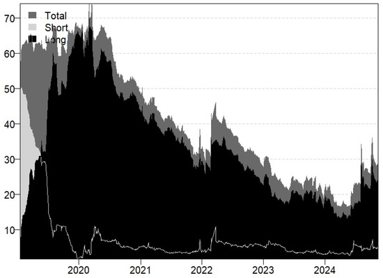
Figure 2.
Dynamic Total Connectedness Index (Total: Dark Gray, Long Term: Black, Short Term: Gray).
To interpret the most significant fluctuations in TCI, it is imperative to contextualize them within major global events that unfolded between 2019 and 2024. The dynamic nature of TCI emphasizes the responsiveness of financial linkages to economic crises and external shocks, reinforcing its role as a leading metric for assessing systemic risk. The graphical representation reveals considerable fluctuations over time, characterized by sharp peaks and troughs that signal shifts in financial interdependence.
Periods of heightened TCI values correspond to phases of elevated systemic risk, where financial assets exhibit strong co-movement, often triggered by global economic disruptions, geopolitical tensions, or policy changes. Short-term surges in TCI generally reflect immediate market reactions to external shocks, while sustained long-term interdependencies suggest deeper structural financial linkages within the system.
Monitoring TCI fluctuations is particularly relevant for investors and policymakers, as elevated levels act as early warning signals of financial instability. During financial crises, short-term volatility spillovers tend to dominate, capturing abrupt market responses to disruptions. In contrast, long-term spillovers provide valuable insights into persistent structural vulnerabilities, guiding the formulation of risk mitigation strategies and enhancing macro-prudential oversight. By distinguishing between temporary market shocks and enduring systemic risks, TCI serves as a vital tool in navigating financial uncertainty and reinforcing market resilience.
The figure illustrates significant peaks in the Total Connectedness Index (TCI), particularly in early 2020 and early 2022, with values exceeding 60 during these periods. While both short-term and long-term interconnectedness also rise, their fluctuations are less pronounced compared to total TCI. From the second half of 2020 onward, TCI exhibits a gradual downward trend, stabilizing at lower levels throughout 2023. This decline suggests a weakening of global financial interconnectedness, with market dynamics increasingly shaped by regional factors rather than broad-based global shocks.
The surge in early 2020 aligns with the onset of the COVID-19 pandemic, which caused severe disruptions in economic and financial systems worldwide. Rising global uncertainty and market volatility heightened financial interdependence, reflected in the sharp increase in TCI during this period. The escalation in short-term TCI underscores immediate market responses to pandemic-induced shocks, whereas the sustained rise in long-term TCI suggests that the crisis had lasting economic implications, influencing macroeconomic fundamentals beyond the initial shock.
A similar pattern emerges in early 2022 with the Russia–Ukraine war, which profoundly impacted energy and commodity markets, particularly those with direct exposure to European and Russian trade flows. Uncertainty surrounding global energy supply chains drove heightened market volatility, leading to another surge in Total TCI. This increase illustrates how geopolitical risks propagate through financial networks, amplifying systemic volatility across interconnected markets. Economies heavily reliant on energy price stability, such as Russia’s MOEX, absorbed significant external shocks, reinforcing the rise in TCI during this period.
By 2023, TCI stabilizes at lower levels, reflecting the gradual dissipation of pandemic-related disruptions, a relative recovery in global economic conditions, and a shift toward more localized financial dynamics. The decline in Total TCI indicates a weakening of global financial interdependence, with volatility increasingly driven by domestic and regional factors rather than systemic global shocks. The persistently low short-term TCI values in 2023 and beyond further suggest that sudden global shocks exert a diminishing influence, with financial movements primarily dictated by localized economic and geopolitical developments. Conversely, long-term TCI fluctuations continue to reflect the persistent influence of macroeconomic trends and policy decisions on market volatility. For example, the lasting economic consequences of the pandemic and fluctuations in global energy prices remain key determinants of financial market stability. Peaks in long-term TCI highlight the role of fundamental macroeconomic variables, including fiscal policies, interest rate adjustments, and shifts in global trade dynamics, in shaping extended volatility cycles.
2.3.3. Net Total Directional Connectedness
Figure 3 illustrates the dynamic Net Total Directional Connectedness (NET) indices, capturing the evolving transmission and absorption of volatility across financial markets. Consistent with connectedness theory, global crises and country-specific economic developments determine whether a market serves as a volatility transmitter or receiver. As seen in the Total Connectedness Index (TCI) analysis, NET indices highlight two major global events: the COVID-19 pandemic (March 2020) and the Russia–Ukraine war (February 2022). Both crises triggered sharp volatility surges, fundamentally altering financial interconnectedness.
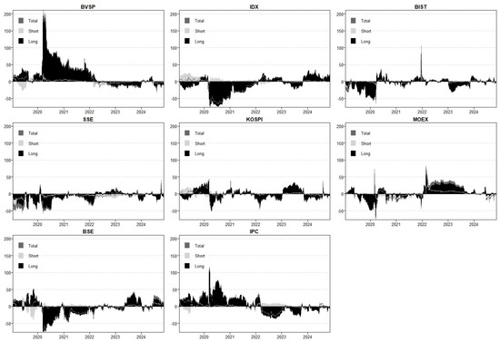
Figure 3.
Net Total Directional Connectedness (Total: Dark Gray, Long Term: Black, Short Term: Gray).
Amongst the analyzed markets, BVSP emerges as the strongest volatility transmitter, reaching a peak NET value of 210.76% on 18 March 2020. This extreme figure underscores Brazil’s role in propagating financial shocks, largely due to its dependence on energy and agricultural commodities. Volatility spillovers intensify during global crises when commodity price fluctuations exacerbate systemic uncertainty. The persistently high long-term NET values of BVSP following the COVID-19 pandemic further confirm its role as a major volatility spreader, particularly through commodity price shocks. However, after the Russia–Ukraine war, BVSP’s NET values stabilized near zero, suggesting reduced volatility transmission and greater resilience. A similar transmission pattern is evident in IPC, portraying high sensitivity to global economic shocks due to its strong energy and commodity market linkages. This dependency results in consistently positive NET values, positioning IPC as a volatility transmitter across both short- and long-term horizons. The COVID-19 pandemic reinforced IPC’s role in systemic risk transmission, mirroring BVSP’s behavior.
The parallel volatility patterns in Latin American markets indicate a regional spillover effect, where external shocks spread rapidly across economies with commodity-driven financial structures. In contrast, SSE and IDX consistently exhibit negative NET values, indicating that they absorb rather than transmit volatility. The Shanghai Stock Exchange has functioned as a volatility receiver, reflecting China’s controlled financial structure and limited external exposure. The negative NET values of SSE over long time horizons suggest that volatility in the Chinese market is largely externally driven rather than rooted in domestic instability. Similarly, IDX remains highly susceptible to shocks in energy and raw material prices, reinforcing its volatility-receiving role. While IDX occasionally exhibits positive NET values in the short term, the prevailing trend confirms its function as a volatility absorber rather than a spreader within the global financial system.
Unlike markets that consistently function as either volatility transmitters or receivers, BIST assumes a dual role, exhibiting characteristics of both at different points in time. A significant exchange rate shock in December 2021 triggered a sharp increase in BIST’s NET values, positioning it as a short-term volatility transmitter. This spike was primarily driven by exchange rate fluctuations, monetary policy adjustments, and investor uncertainty, which led to substantial disruptions in local financial markets. Türkiye’s volatility dynamics were further shaped by the Kahramanmaraş earthquakes in February 2023, which introduced additional short-term financial shocks. However, this effect remained largely localized, suggesting that BIST’s role in systemic volatility transmission is contingent on the nature of the shock. Over longer time horizons, Türkiye exhibits a more integrated financial structure, making it more susceptible to external volatility spillovers rather than serving as a primary source of global systemic risk.
The Russia–Ukraine war of February 2022 marked a pivotal shift in the volatility dynamics of MOEX. On the day the conflict began, MOEX recorded a sharp increase in NET values, establishing itself as a significant volatility transmitter. This surge reflects the immediate impact of geopolitical uncertainty, capital outflows, and heightened financial risk perceptions surrounding Russian assets. However, the post-war imposition of economic sanctions and the partial closure of the Moscow Exchange fundamentally altered MOEX’s role in global financial networks. As a result, MOEX transitioned into a volatility-receiving market, becoming more vulnerable to external shocks rather than actively spreading systemic risk. This transition underscores the profound effects of geopolitical developments on financial market stability and connectedness.
BSE has demonstrated positive NET values across both short- and long-term horizons, highlighting its growing influence as a volatility transmitter. India’s increasing role in global trade, foreign investment flows, and energy markets has amplified its importance in financial interconnectedness. Notably, BSE’s NET values intensified during the COVID-19 pandemic, reflecting its heightened sensitivity to commodity price fluctuations and global market uncertainty. This trend suggests that as India continues to integrate into global financial networks, its role as a source of systemic volatility spillovers is likely to expand, particularly during periods of economic distress.
Ultimately, the findings reveal the following key patterns: Markets exhibiting positive NET values, such as BVSP, IPC, and BSE, serve as primary sources of systemic volatility, particularly due to their exposure to commodity price fluctuations and global economic uncertainty. Markets with negative NET values, including SSE and IDX, predominantly absorb external shocks rather than transmit them, reflecting their structural characteristics and economic policies. Türkiye’s BIST alternates between volatility transmission and absorption, with short-term spikes driven by domestic shocks (e.g., exchange rate fluctuations and natural disasters) and long-term integration with global financial trends. MOEX’s shift from volatility transmitter to receiver illustrates how geopolitical events and economic sanctions can redefine a market’s role in systemic risk transmission.
2.3.4. Dynamic NPDC and PCI Analyses
This section examines the findings from the dynamic NPDC and PCI analyses, presented in Figure 4 and Figure 5, respectively. These analyses provide detailed insights into volatility spillovers and market interactions in global financial systems. Bilateral market connections fluctuate over time but become particularly pronounced during periods of crisis. Notably, Brazil’s BVSP index stands out as a dominant volatility spreader in both NPDC and PCI analyses. A persistent and strong interaction is observed between BVSP and Mexico’s IPC index, reflecting regional integration and a shared commodity-based economic structure. Similarly, Brazil’s connection with India’s BSE index exhibits a positive relationship due to trade in commodities. However, its ties to Asian markets such as China (SSE) and Indonesia (IDX) are weaker. PCI values for these market pairs remain low, with temporary increases observed only during global crises, such as the COVID-19 pandemic. NPDC findings further support this pattern: while Brazil transmits volatility to China and Indonesia, it receives minimal volatility from these economies. This reflects China’s controlled financial structure and Indonesia’s vulnerability to external shocks.

Figure 4.
Net Pairwise Directional Connectedness (Total: Dark Gray, Long Term: Black, Short Term: Gray).
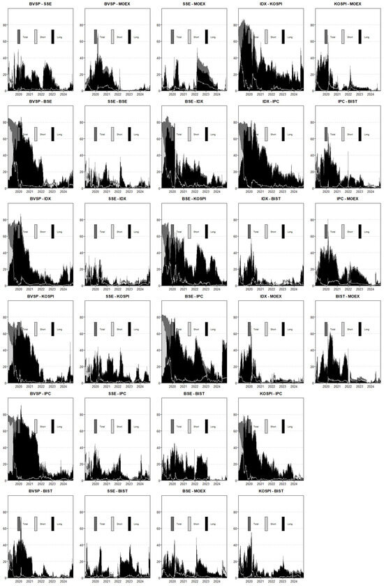
Figure 5.
Pairwise Connectedness Index (Total: Dark Gray, Long Term: Black, Short Term: Gray).
Russia’s MOEX index underwent a notable shift during the 2022 Russia–Ukraine war. During this period, MOEX experienced a surge in PCI values, briefly acting as a volatility transmitter. However, following the imposition of sanctions and market restrictions, MOEX reverted to a volatility-receiving role in the long term. A similar dynamic is observed between Türkiye’s BIST index and MOEX. Given Russia’s influence in energy markets and Türkiye’s reliance on energy imports, PCI values between the two markets rose significantly during crisis periods. NPDC graphs further confirm that Türkiye alternates between being a volatility receiver and transmitter, depending on market conditions.
In Asian markets, China (SSE) and South Korea (KOSPI) exhibit greater sensitivity to external shocks and generally function as volatility receivers in NPDC analyses. However, energy-based connectivity is evident between China and Russia, particularly during crises, as reflected in PCI spikes. By contrast, South Korea and Mexico (IPC) exhibit minimal financial interconnectedness, likely due to fundamental differences in their economic structures. While South Korea’s economy is driven by technology and manufacturing, Mexico’s is more commodity- and energy-dependent, resulting in low PCI and NPDC values between the two markets.
When evaluated together, NPDC and PCI analyses provide a clearer understanding of how market connectivity evolves in both directionality and intensity. While positive NPDC values indicate the direction of volatility spillovers between specific market pairs, PCI quantifies the overall strength of these linkages and their fluctuations during crisis periods. Global shocks such as the COVID-19 pandemic and the Russia–Ukraine war have triggered temporary surges in PCI values, making inter-market relationships more pronounced. Latin American markets display stronger financial integration, whereas Asian markets remain more fragile and highly sensitive to external shocks. A closer examination of Brazil’s BVSP index highlights term-dependent variations in its volatility spillover effects. Over the long term, BVSP consistently exhibits dominant NPDC values, reinforcing its role as a major volatility transmitter. However, when considering total values, BVSP acts as a volatility receiver relative to KOSPI. Furthermore, BVSP and IPC register the highest average PCI values in the financial network, confirming their significance as key volatility spreaders. These findings underscore the importance of distinguishing between short-term and long-term spillover effects in understanding the broader dynamics of financial interconnectedness.
2.3.5. Average NPDC and PCI Analyses
Table 3 presents the NPDC and PCI values, which quantify both the direction and intensity of market interconnectedness. It is evident that BVSP acts as a dominant volatility transmitter across all markets, with IDX (4.20%) and BSE (4.19%) experiencing the highest spillovers, highlighting BVSP’s influence on Asian (India and Indonesia), Russian (MOEX), and Latin American (Mexico) markets. In contrast, SSE (China) receives the least volatility (1.06%), and KOSPI (1.48%) and BIST (1.70%) register relatively low NPDC values, indicating weaker transmission to these markets. PCI values further illustrate BVSP’s strongest financial linkages, particularly with Mexico (37.16%), India, South Korea, and Indonesia. The exceptionally high PCI value with Mexico suggests a strong degree of integration, likely due to geographic proximity and shared geopolitical risks. Conversely, MOEX (13.07%), BIST (15.48%), and SSE (15.95%) exhibit weaker connectivity with BVSP, reinforcing the notion that Brazil’s influence on Russia is more indirect, driven by commodity and energy price interactions rather than direct financial ties. Given that BVSP spreads the most volatility to Indonesia, India, and Russia, investments in these markets may be particularly sensitive to Brazil-driven fluctuations.
Table 3.
Average NPDC and PCI.
Since Mexico maintains the highest PCI value with BVSP, these two markets tend to move in tandem. India, Indonesia, and South Korea, which also exhibit high PCI values with BVSP, may serve as regional diversification options, linking Latin American and Asian markets. In contrast, China and Türkiye, which show weak PCI connections to BVSP, may provide portfolio balance and risk mitigation benefits. Short-term NPDC dynamics suggest BVSP is more passive against markets with strong long-term and aggregate bilateral connectivity. Markets that act as volatility receivers with high PCI values include BSE (−0.39% | 9.59%), KOSPI (−0.44% | 6.17%), IDX (−0.76% | 6.08%), and IPC (−0.25% | 8.00%). In contrast, BVSP dominates volatility transmission to BIST, SSE, and MOEX in the short term, making investments in these markets more exposed to Brazil-driven fluctuations. Since Türkiye and Russia exhibit very low PCI values, they tend to operate independently from BVSP, positioning them as alternative diversification assets. Meanwhile, Brazil’s strong correlation with India and Mexico suggests that these markets exhibit parallel movements, potentially creating arbitrage opportunities for short-term investors monitoring Brazil-India and Brazil-Mexico price dynamics.
KOSPI exhibits strong connectivity with IDX (−1.29% | 37.99%), where it acts as a volatility receiver, while BSE (0.34% | 37.12%) is a transmitter with a high bilateral connection. Additionally, KOSPI maintains a relatively strong relationship with BVSP (−1.48% | 30.52%) and IPC (0.18% | 29.43%), while its ties to SSE (15.24%), BIST (12.50%), and MOEX (11.25%) are comparatively weaker. Overall, KOSPI is highly interconnected with BSE, BVSP, and IDX but exhibits limited linkages with MOEX and BIST in both the short and long term. Since IDX and BSE exhibit high PCI values, including them in the same portfolio may amplify risk. Conversely, markets with low PCI values, such as SSE, MOEX, and BIST, could serve as diversification assets in a KOSPI-based portfolio. Given that BVSP and IDX are the primary sources of long-term volatility for KOSPI, monitoring their interrelations is crucial for investment strategies.
IDX is one of the most affected markets by volatility transmission from IPC and BVSP, while it spreads volatility to KOSPI and SSE. In the short term, IDX transmits heightened volatility to BSE and IPC and continues to do so over the long term, maintaining a parallel pattern to short-term bilateral relationships. While IDX shares high volatility with BSE and IPC in the short term, its strongest long-term bilateral connections are with IPC and KOSPI. SSE, contrarily, demonstrates low connectivity across all markets. The lowest PCI value in total is observed between SSE and IDX (−1.23% | 8.81%), indicating minimal direct linkages.
SSE functions as a net transmitter only in relation to BIST, though this connection is negligible, with 0.01% NPDC and 1.54% PCI, suggesting that SSE and BIST have almost no financial interdependence in the short term. However, SSE dominates BIST in the long term. While BIST has the highest NPDC value in the short term, MOEX (−0.32% | 2.12%) remains largely disconnected from other markets, positioning it as a neutral market. The BIST-MOEX relationship can be attributed to geographical proximity and Türkiye’s dependence on Russian energy imports. While BIST dominates MOEX in the long term, it acts as a receiver in the short term. MOEX’s neutral position stems from its heavy reliance on internal factors, as reflected in its high internal PCI value of 49.9% in the short term. This underscores the dominance of Russia’s domestic market conditions over external influences, a factor further reinforced by geopolitical risks and international sanctions.
SSE’s low NPDC and PCI values suggest that it operates as a relatively independent market within the global financial network. While this insulation offers diversification benefits, it also limits arbitrage opportunities for investors. Capital controls and regulatory policies likely restrict SSE’s role in global market integration. Despite being one of the world’s largest exchanges by market capitalization, SSE functions differently from other major financial centers due to China’s strict capital market regulations, deep liquidity, and a predominantly local investor base. Unlike smaller, open economies, large exchanges with deep internal liquidity tend to be less vulnerable to global fluctuations. SSE’s low NPDC value reinforces its status as a self-contained financial ecosystem rather than a net volatility transmitter. Additionally, its relatively low PCI value further indicates that China’s stock market does not fully transmit or absorb global financial shocks, most likely due to capital controls. While global equity markets often exhibit strong correlations during major crises, China’s stock market might at times follow a more isolated trajectory.
2.3.6. Network Plots
In the network graphs presented in Figure 6, Figure 7, Figure 8 and Figure 9, dark gray nodes represent dominant volatility transmitters, while light gray nodes denote passive receivers. Arrows pointing toward a node indicate volatility reception, whereas arrows originating from a node signify volatility transmission. The thickness of the arrows reflects the strength of the relationship, while node size corresponds to the magnitude of contagion. Figure 6 identifies BVSP (Brazil) as the largest node in the time domain, reinforcing its position as the primary driver of volatility transmission. Other significant transmitters include IPC (Mexico), MOEX (Russia), and KOSPI (South Korea), all represented as dark-colored nodes. Amongst these, MOEX exhibits strong contagion toward SSE (China), which functions as the largest receiver in the network. In the short term, IDX (Indonesia) emerges as the most dominant transmitter, while SSE remains the largest receiver. Notably, BVSP appears passive in the short term but reasserts its dominance in the long run. The most pronounced contagion effects are observed from MOEX to SSE across both short- and long-term horizons, while IPC and IDX maintain strong long-term connectivity. Meanwhile, BIST (Turkey) exhibits weak integration within the network and primarily functions as a volatility receiver.
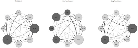
Figure 6.
Network Plot for Whole Period.
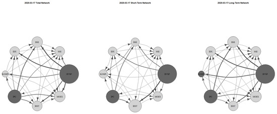
Figure 7.
Network Plot for 17 March 2020.

Figure 8.
Network Plot for 24 February 2022 (Russo–Ukraine War).
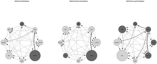
Figure 9.
Network Plot for 24 February 2022 (MOEX reopened).
On 11 March 2020, the day the World Health Organization declared the COVID-19 pandemic, Total TCI surged to 70.35%. It peaked at 73.99% (Short 7.04% + Long 66.95%) on 17 March 2020. Figure 7 presents the network analysis for this date, highlighting BVSP as the dominant exchange in both short- and long-term horizons. Strong volatility transmission is observed from BVSP to BIST in the short term and to BSE and IDX in the long term, confirming that BVSP drives the network. Meanwhile, SSE remains the most passive market, consistently acting as a receiver against all exchanges, while IPC emerges as another key volatility transmitter.
Figure 8 depicts the network structure on the first day of the Russia–Ukraine war, while Figure 9 illustrates bilateral network connectivity when MOEX reopened on 24 March 2022, following a temporary closure. These dates mark peak dynamic TCI values as systemic risk, which had declined post-pandemic, surged again with the onset of the conflict. MOEX led volatility transmission on both dates, with high spillovers to BSE (India) in the long term and to BVSP (Brazil) in the short term. As in previous observations, SSE remains a dominant receiver. When MOEX resumed trading, it once again acted as a major risk transmitter, with strong contagion to SSE in the short term. On this day, BVSP was a major volatility receiver, remaining passive against all markets.
3. Conclusions
The paper herein applies the GK range-based volatility estimator, which utilizes OHLC price data, to analyze stock market fluctuations from 2019 to 2024, integrating a TVP-VAR frequency connectedness framework to evaluate systemic volatility transmission. Our findings reveal that volatility surged during the COVID-19 pandemic, with BVSP (Brazil) and IPC (Mexico) emerging as dominant volatility spreaders. However, geopolitical and macroeconomic developments, particularly the Russo–Ukrainian war and the 2024 U.S. elections, triggered additional volatility increases. Unlike most markets, MOEX (Russia) recorded its highest volatility during the war rather than the pandemic, emphasizing the unique role of geopolitical shocks in financial instability. The Total Connectedness Index (TCI) peaked in early 2020 (pandemic onset) and early 2022 (Russo–Ukrainian war), demonstrating that extreme financial disruptions drive systemic risk transmission.
These findings diverge from Polat [9] and Medetoğlu [13], who found that South Africa and India played a more central role in volatility transmission within BRICS and BRICS-T markets. In contrast, our study positions BVSP and IPC as the dominant volatility spreaders, suggesting that Latin American markets, rather than BRICS economies, currently drive emerging market volatility spillovers. This aligns with Panda et al. [70] and is further supported by Gökgöz et al. [71], who found Brazil to be a significant transmitter of volatility, especially under stress scenarios. Similarly, Kayral et al. [72], using a quantile-frequency approach, confirm Brazil’s resilience and strong outbound transmission during turbulent periods.
Our NET connectedness analysis refines the understanding of market roles. BVSP recorded the highest NET volatility transmission, surging to 210.76% on 18 March 2020, reinforcing its position as a leading transmitter. Türkiye’s BIST alternated between transmitter and receiver roles, responding to localized shocks such as currency devaluations (December 2021) and the Kahramanmaraş earthquakes (February 2023). The fluctuating role of BIST mirrors the findings of Bozma et al. [6] and M. Umer et al. [40], who noted that Turkey and Brazil often shift between volatility sources and receivers in response to economic cycles. Furthermore, Asafo-Adjei et al. [28] and Sayed and Charteris [30] highlight that such cyclical roles are common among segmented and less integrated markets—a characterization that fits BIST’s pattern. However, unlike Gemici [73], who found Mexico and Brazil to be the main financial risk transmitters among E7 markets, our results emphasize Brazil’s unique influence among select EAGLE constituents, with Mexico assuming a comparably stronger contagion role than in prior studies.
Moreover, our NPDC and PCI analyses provide additional insight into bilateral volatility relationships. BVSP exhibits strong contagion effects, particularly with IPC (Mexico), confirming the strong financial integration within Latin America, as also highlighted by Panda et al. [70]. This regional tightness was less emphasized in wavelet-based studies such as Batondo and Uwilingiye [32], who found Brazil’s co-movement with the U.S. more pronounced than with regional partners. Our study extends this understanding by demonstrating the growing importance of intra-Latin American volatility spillovers.
However, our findings diverge from Sarathkumara et al. [11] and Li et al. [5], who identified NASDAQ and NIFTY50 as dominant contagion transmitters in Asia-Pacific markets. While previous studies emphasized Asia’s increasing role in financial contagion, our results indicate that Latin American markets currently hold a more dominant role in volatility transmission than traditionally assumed. This contrast suggests a shifting dynamic in global financial networks, where Brazil and Mexico’s spillover effects are becoming more influential relative to traditional Asian financial hubs. Our evidence is also distinct from Yüzbaşıoğlu [74], who found stronger long-term connectedness among BRICS via wavelet correlation, with China partially segmented. Conversely, our analysis shows that China’s SSE remains largely insulated, recording the lowest total connectivity (8.81%) with IDX (Indonesia), reinforcing Chow [75] and Dahir et al. [18], who found that China remains a net receiver of financial volatility due to strict capital controls and deep internal liquidity. However, our study contradicts Wiesen et al. [76], who argue that China exerts an indirect but substantial impact on regional financial markets. Instead, we confirm that China’s financial system operates largely in isolation, with minimal direct linkages to major volatility spreaders such as BVSP and IPC.
Furthermore, MOEX’s volatility behavior presents another key divergence from past research. Unlike studies such as Mateus et al. [22], Bejaoui et al. [77], and Belcaid et al. [78], which found Russia to be a key volatility transmitter within Eurasian markets, our results indicate that MOEX transitioned into a volatility-receiving role post-2022. This shift reflects the impact of geopolitical risks, economic sanctions, and restricted market access, which have structurally altered Russia’s financial dynamics. Our findings align with Xu et al. [79], who demonstrated that emerging economies like Russia are more vulnerable to external financial shocks than previously thought.
Our study has important implications for key stakeholders, including academics, policymakers, regulatory bodies, and investors. For academics, our study extends the literature by demonstrating that Latin American markets (BVSP and IPC) have overtaken traditional BRICS markets as leading volatility transmitters. This finding challenges previous research that emphasized Asian and Eurasian dominance in volatility transmission. Furthermore, our application of the TVP-VAR frequency connectedness approach provides a dynamic framework that can be expanded to study sectoral financial spillovers or other asset classes, such as bonds and commodities. For policymakers and regulatory bodies, our results underscore the need for enhanced financial oversight in highly connected markets. Countries such as Brazil and Mexico require macro-prudential safeguards, including liquidity buffers and circuit breakers, to mitigate the amplification of systemic risks. These recommendations align with previous studies such as Oral and Özkan [80], who emphasized that financial regulators in emerging markets must strengthen systemic risk mitigation mechanisms. Additionally, our findings call for a reassessment of capital controls in China, as the SSE’s extreme insulation may limit its global financial efficiency rather than enhance its stability. For investors and portfolio managers, our findings highlight key volatility spreaders and receivers, which are critical for hedging and diversification strategies. BVSP and IPC exhibit strong co-movement, indicating that investments in these markets require correlation-based risk assessments. Meanwhile, SSE’s low connectivity presents hedging opportunities against global market shocks, while BIST’s fluctuating role suggests exposure to local geopolitical risks. Our findings reinforce Dang et al. [81], who showed that commodity-driven emerging markets (e.g., MOEX, IDX) require commodity price volatility adjustments in portfolio allocation strategies.
All in all, this study contributes to the literature by documenting a fundamental realignment in global volatility transmission, wherein Latin America, led by Brazil and Mexico, has displaced traditional BRICS and Asia-Pacific markets as the core sources of systemic financial spillovers. By leveraging a TVP-VAR frequency-domain framework on EAGLE sample, this paper fills a methodological gap in the literature, offering bilateral, time-varying, and multi-frequency volatility connectedness insights. Prior studies often relied on static frameworks (e.g., DCC-GARCH, wavelet coherence) or quantile-only spillover models, which, while insightful, did not jointly capture the evolving direction and intensity of spillovers across different time horizons. Furthermore, our findings diverge from the consensus that positioned China, South Africa, or India as dominant volatility hubs. Instead, Brazil and Mexico now emerge as central to global contagion dynamics. MOEX’s reversal into a net receiver and SSE’s isolation reinforce the idea that geopolitical constraints and policy insulation can significantly reshape financial interdependence. These findings offer timely insights for academics, market participants, and policymakers seeking to manage systemic risk in an increasingly interconnected and crisis-prone financial landscape.
Author Contributions
Conceptualization, H.K.; Methodology, Y.A., H.K. and H.U.; Software (R version 4.3.3), Y.A.; Validation, H.U.; Formal analysis, Y.A.; Investigation, H.U.; Resources, Y.A. and H.K.; Data curation, Y.A.; Writing—original draft, H.K.; Writing—review and editing, H.K.; Visualization, Y.A.; Supervision, H.U.; Project administration, H.U. All authors have read and agreed to the published version of the manuscript.
Funding
This research received no external funding.
Data Availability Statement
Data derived from https://finance.yahoo.com/ and https://www.investing.com/ (accessed on 17 January 2025).
Acknowledgments
The authors would like to thank the referees for their valuable comments that improved the manuscript herein.
Conflicts of Interest
The authors declare no conflicts of interest.
References
- Attarzadeh, A.; Balcilar, M. On the dynamic connectedness of the stock, oil, clean energy, and technology markets. Energies 2022, 15, 1893. [Google Scholar] [CrossRef]
- Mensi, W.; Maitra, D.; Selmi, R.; Tiwari, A.K.; Vo, X.V. Extreme dependencies and spillovers between gold and stock markets: Evidence from MENA countries. Financ. Innov. 2023, 9, 47. [Google Scholar] [CrossRef] [PubMed]
- Raddant, M.; Kenett, D.Y. Interconnectedness in the global financial market. J. Int. Money Financ. 2021, 110, 102280. [Google Scholar] [CrossRef]
- Dsouza, S.; Singh, N.P.; Oliyide, J.A. Dynamic connectedness among the BRICS markets and the recent pandemic: An application of TVP-VAR approach. Int. J. Emerg. Mark. 2024. [Google Scholar] [CrossRef]
- Li, Y.; Shi, Y.; Shi, Y.; Xiong, X.; Yi, S. Time-frequency extreme risk spillovers between COVID-19 news-based panic sentiment and stock market volatility in the multi-layer network: Evidence from the RCEP countries. Int. Rev. Financ. Anal. 2024, 94, 103339. [Google Scholar] [CrossRef]
- Bozma, G.; İmamoğlu, İ.K.; Künü, S. Dynamic volatility spillover among emerging EAGLE markets. Ekon. Sos. Araşt. Derg. 2023, 19, 316–336. [Google Scholar]
- Khan, M.A.; Khan, M.A.; Ahmed, M.; Khan, K. Environmental consequences of financial development in emerging and growth-leading economies: A multidimensional assessment. Borsa Istanb. Rev. 2022, 22, 668–677. [Google Scholar] [CrossRef]
- Tabash, M.I.; Farooq, U.; Anagreh, S.; Al-Faryan, M.A.S. Contributing to sustainable development goals (SDGs) in environmental sustainability through public-private investment in energy: Empirical evidence from EAGLE economies. Int. J. Innov. Sci. 2024, 16, 838–854. [Google Scholar] [CrossRef]
- Polat, O. Dynamic network connectedness of BRICS equity markets during the COVID-19 era. Ömer Halisdemir Univ. Iktisadi Idari Bilim. Fak. Derg. 2021, 14, 1486–1498. [Google Scholar] [CrossRef]
- Liu, Z.; Ji, Q.; Zhai, P.; Ding, Z. Asymmetric and time-frequency volatility connectedness between China and international crude oil markets with portfolio implications. Res. Int. Bus. Financ. 2023, 66, 102039. [Google Scholar] [CrossRef]
- Sarathkumara, S.M.N.N.; Samarakoon, S.M.R.K.; Pradhan, R.P. Navigating financial interconnectivity: Analyzing oil, exchange rates and US market influences on Asia-Pacific equities using the time-varying parameter vector autoregressive connectedness approach. J. Econ. Stud. 2025; ahead of print. [Google Scholar] [CrossRef]
- Deléchat, C.; Rawat, U.; Stepanyan, A. Navigating External Shocks in Southeast Asia’s Emerging Markets: Key Lessons and Challenges in Applying the IMF’s Integrated Policy Framework; IMF Departmental Paper No. DP/2024/007; International Monetary Fund: Washington, DC, USA, 2024. [Google Scholar]
- Medetoğlu, B. TVP-VAR yöntemi ile dinamik bağlantılılık tespiti: CIVETS ülkeleri üzerine uygulama. Pamukkale Univ. Sos. Bilim. Enst. Derg. 2024, 61, 17–34. [Google Scholar] [CrossRef]
- Yousaf, I.; Youssef, M.; Goodell, J.W. Tail connectedness between artificial intelligence tokens, artificial intelligence ETFs, and traditional asset classes. J. Int. Financ. Mark. Inst. Money 2024, 91, 101929. [Google Scholar] [CrossRef]
- Aziz, M.I.A.; Ahmad, N.; Zichu, J.; Nor, S.M. The impact of COVID-19 on the connectedness of stock index in ASEAN+3 economies. Mathematics 2022, 10, 1417. [Google Scholar] [CrossRef]
- López Herrera, F.; Santillán Salgado, R.J.; Cruz Aké, S. Volatility dependence structure between the Mexican Stock Exchange and the world capital market. Inv. Econ. 2015, 74, 5–33. [Google Scholar] [CrossRef]
- Trevino Aguilar, E. The interdependency structure in the Mexican stock exchange: A network approach. PLoS ONE 2020, 15, e0238731. [Google Scholar] [CrossRef] [PubMed]
- Dahir, A.M.; Mahat, F.; Amin Noordin, B.-A.; Hisyam Ab Razak, N. Dynamic connectedness between Bitcoin and equity market information across BRICS countries: Evidence from TVP-VAR connectedness approach. Int. J. Manag. Financ. 2020, 16, 357–371. [Google Scholar] [CrossRef]
- Altınkeski, B.K.; Dibooglu, S.; Cevik, E.I.; Kılıç, Y.; Bugan, M.F. Quantile connectedness between VIX and global stock markets. Borsa Istanb. Rev. 2024, 24 (Suppl. 1), 71–79. [Google Scholar] [CrossRef]
- Lee, H.S.; Lee, W.S. Housing market volatility connectedness among G7 countries. Appl. Econ. Lett. 2018, 25, 146–151. [Google Scholar] [CrossRef]
- Tessmann, M.; Gutiérrez, C.E.C.; Khodr, O.; Magalhães, L.A.; Passos, M.D.O. Volatility transmission and market connectivity of metals and energy commodities: Insights from the spillover index. Int. J. Energy Econ. Policy 2024, 14, 609–618. [Google Scholar] [CrossRef]
- Mateus, C.; Bagirov, M.; Mateus, I. Return and volatility connectedness and net directional patterns in spillover transmissions: East and Southeast Asian equity markets. Int. Rev. Financ. 2024, 24, 83–103. [Google Scholar] [CrossRef]
- Vo, D.H.; Dang, T.H.N. The geopolitical risk spillovers across BRICS countries: A quantile frequency connectedness approach. Scott. J. Polit. Econ. 2024, 71, 132–143. [Google Scholar] [CrossRef]
- Agyei, S.K.; Owusu Junior, P.; Bossman, A.; Asafo-Adjei, E.; Asiamah, O.; Adam, A.M. Spillovers and contagion between BRIC and G7 markets: New evidence from time-frequency analysis. PLoS ONE 2022, 17, e0271088. [Google Scholar] [CrossRef] [PubMed]
- Baruník, J.; Křehlík, T. Measuring the frequency dynamics of financial connectedness and systemic risk. J. Financ. Econom. 2018, 16, 271–296. [Google Scholar] [CrossRef]
- Shi, K. Spillovers of stock markets among the BRICS: New evidence in time and frequency domains before the outbreak of COVID-19 pandemic. J. Risk Financ. Manag. 2021, 14, 112. [Google Scholar] [CrossRef]
- Khan, Z.; Khan, K.H.; Koch, H. Aggregating an economic model and GIS to explore trade potentials of India-Caspian countries and a way forward for INSTC. Res. Glob. 2023, 7, 100154. [Google Scholar] [CrossRef]
- Asafo-Adjei, E.; Adam, A.M.; Adu-Asare Idun, A.; Ametepi, P.Y. Dynamic interdependence of systematic risks in emerging markets economies: A recursive-based frequency-domain approach. Discret. Dyn. Nat. Soc. 2022, 2022, 1139869. [Google Scholar] [CrossRef]
- Anyikwa, I.C.; Phiri, A. Dynamics of return and volatility spill-over between developed, emerging and African equity markets during the COVID-19 pandemic and Russia–Ukraine war. Stud. Econ. Econom. 2023, 47, 144–168. [Google Scholar] [CrossRef]
- Sayed, A.; Charteris, A. Integration among the BRICS stock markets: Filtering out global factors. Invest. Anal. J. 2024, 53, 207–230. [Google Scholar] [CrossRef]
- Gurdgiev, C.; O’Riordan, C. A wavelet perspective of crisis contagion between advanced economies and the BRIC markets. J. Risk Financ. Manag. 2021, 14, 503. [Google Scholar] [CrossRef]
- Batondo, M.; Uwilingiye, J. Comovement across BRICS and the US stock markets: A multitime scale wavelet analysis. Int. J. Financ. Stud. 2022, 10, 27. [Google Scholar] [CrossRef]
- Mensi, W.; Sensoy, A.; Aslan, A.; Kang, S.H. High-frequency asymmetric volatility connectedness between Bitcoin and major precious metals markets. N. Am. J. Econ. Financ. 2019, 50, 101031. [Google Scholar] [CrossRef]
- Baruník, J.; Kočenda, E.; Vácha, L. Asymmetric volatility connectedness on the forex market. J. Int. Money Financ. 2017, 77, 39–56. [Google Scholar] [CrossRef]
- Wan, Y.; Song, Y.; Zhang, X.; Yin, Z. Asymmetric volatility connectedness between cryptocurrencies and energy: Dynamics and determinants. Front. Environ. Sci. 2023, 11, 1115200. [Google Scholar] [CrossRef]
- Shaik, M.; Varghese, G.; Madhavan, V. The dynamic volatility connectedness of global financial assets during the Ebola & MERS epidemic and the COVID-19 pandemic. Appl. Econ. 2023, 55, 880–900. [Google Scholar] [CrossRef]
- Alrweili, H.; Ben-Salha, O. Dynamic asymmetric volatility spillover and connectedness network analysis among sectoral renewable energy stocks. Mathematics 2024, 12, 1816. [Google Scholar] [CrossRef]
- Yang, L. Idiosyncratic information spillover and connectedness network between the electricity and carbon markets in Europe. J. Commod. Mark. 2022, 25, 100185. [Google Scholar] [CrossRef]
- Shahzad, S.J.H.; Naeem, M.A.; Peng, Z.; Bouri, E. Asymmetric volatility spillover among Chinese sectors during COVID-19. Int. Rev. Financ. Anal. 2021, 75, 101754. [Google Scholar] [CrossRef]
- Umer, U.M.; Coskun, M.; Kiraci, K. Time-varying return and volatility spillover among EAGLEs stock markets: A multivariate GARCH analysis. J. Financ. Econ. Res. 2018, 3, 23–42. [Google Scholar] [CrossRef]
- Anwer, Z.; Naeem, M.A.; Hassan, M.K.; Karim, S. Asymmetric connectedness across Asia-Pacific currencies: Evidence from time-frequency domain analysis. Financ. Res. Lett. 2022, 47, 102782. [Google Scholar] [CrossRef]
- Arif, I.; Rawat, A.S. Corruption, governance, and tax revenue: Evidence from EAGLE countries. Emerg. Mark. Financ. Trade 2018, 54, 119–133. [Google Scholar] [CrossRef]
- Khan, M.A.; Kong, D.; Xiang, J.; Zhang, J. Impact of institutional quality on financial development: Cross-country evidence based on emerging and growth-leading economies. Emerg. Mark. Financ. Trade 2019, 55, 3829–3845. [Google Scholar] [CrossRef]
- Arregui, N.; Norat, M.; Pancorbo, A.; Scarlata, J.G.; Holttinen, E.; Melo, F.; Surti, J.; Wilson, C.; Wehrhahn, R.; Yanase, M. Addressing Interconnectedness: Concepts and Prudential Tools; IMF Working Paper No. WP/13/199; International Monetary Fund: Washington, DC, USA, 2013. [Google Scholar]
- Górka, J.; Kuziak, K. Dynamic connectedness among alternative and conventional energy ETFs based on the TVP-VAR approach. Energies 2024, 17, 5929. [Google Scholar] [CrossRef]
- Arı, Y. TVP-VAR based CARR-volatility connectedness: Evidence from the Russian–Ukraine conflict. Ekon. Polit. Finans Araşt. Derg. 2022, 7, 590–607. [Google Scholar] [CrossRef]
- Ulrich, J. TTR: Technical Trading Rules (R Package Version 0.24.4). Comprehensive R Archive Network (CRAN). 2023. Available online: https://CRAN.R-project.org/package=TTR (accessed on 5 April 2025).
- Diebold, F.X.; Yılmaz, K. Financial and Macroeconomic Connectedness: A Network Approach to Measurement and Monitoring; Oxford University Press: Oxford, UK, 2015. [Google Scholar]
- Demirer, M.; Diebold, F.X.; Liu, L.; Yılmaz, K. Estimating global bank network connectedness. J. Appl. Econom. 2018, 33, 1–15. [Google Scholar] [CrossRef]
- D’Agostino, R.B. Transformation to normality of the null distribution of g1. Biometrika 1970, 57, 679–681. [Google Scholar] [CrossRef]
- Anscombe, F.J.; Glynn, W.J. Distribution of the kurtosis statistic b2 for normal samples. Biometrika 1983, 70, 227–234. [Google Scholar] [CrossRef]
- Jarque, C.M.; Bera, A.K. Efficient tests for normality, homoscedasticity and serial independence of regression residuals. Econ. Lett. 1980, 6, 255–259. [Google Scholar] [CrossRef]
- Elliott, G.; Rothenberg, T.J.; Stock, J.H. Efficient tests for an autoregressive unit root. Econometrica 1996, 64, 813–836. [Google Scholar] [CrossRef]
- Fisher, T.J.; Gallagher, C.M. New weighted portmanteau statistics for time series goodness of fit testing. J. Am. Stat. Assoc. 2012, 107, 777–787. [Google Scholar] [CrossRef]
- Diebold, F.X.; Yılmaz, K. Measuring financial asset return and volatility spillovers, with application to global equity markets. Econ. J. 2009, 119, 158–171. [Google Scholar] [CrossRef]
- Diebold, F.X.; Yılmaz, K. Better to give than to receive: Predictive directional measurement of volatility spillovers. Int. J. Forecast. 2012, 28, 57–66. [Google Scholar] [CrossRef]
- Diebold, F.X.; Yılmaz, K. On the network topology of variance decompositions: Measuring the connectedness of financial firms. J. Econom. 2014, 182, 119–134. [Google Scholar] [CrossRef]
- Pesaran, H.H.; Shin, Y. Generalized impulse response analysis in linear multivariate models. Econ. Lett. 1998, 58, 17–29. [Google Scholar] [CrossRef]
- Antonakakis, N.; Chatziantoniou, I.; Gabauer, D. Refined measures of dynamic connectedness based on time-varying parameter vector autoregressions. J. Risk Financ. Manag. 2020, 13, 84. [Google Scholar] [CrossRef]
- Huang, J.; Chen, B.; Xu, Y.; Xia, X. Time-frequency volatility transmission among energy commodities and financial markets during the COVID-19 pandemic: A novel TVP-VAR frequency connectedness approach. Financ. Res. Lett. 2023, 53, 103634. [Google Scholar] [CrossRef] [PubMed]
- Koop, G.; Korobilis, D. Large time-varying parameter VARs. J. Econom. 2013, 177, 185–198. [Google Scholar] [CrossRef]
- Koop, G.; Korobilis, D. A new index of financial conditions. Eur. Econ. Rev. 2014, 71, 101–116. [Google Scholar] [CrossRef]
- Akbulut, N.; Arı, Y. TVP-VAR frequency connectedness between the foreign exchange rates of non-Euro area member countries. Folia Oecon. Stetin. 2023, 23, 1–23. [Google Scholar] [CrossRef]
- Arı, Y.; Kurt, H.; Uçak, H. Volatility connectedness across global e-commerce stocks. Econ. Rev. 2024, 75, 295–310. [Google Scholar] [CrossRef]
- Gabauer, D. ConnectednessApproach: Connectedness Approach, R package version 1.0.4; R Foundation for Statistical Computing: Vienna, Austria, 2022; Available online: https://CRAN.R-project.org/package=ConnectednessApproach (accessed on 26 January 2025).
- Koop, G.; Pesaran, M.H.; Potter, S.M. Impulse response analysis in nonlinear multivariate models. J. Econom. 1996, 74, 119–147. [Google Scholar] [CrossRef]
- Long, S.; Chatziantoniou, I.; Gabauer, D.; Lucey, B. Do social media sentiments drive cryptocurrency intraday price volatility? New evidence from asymmetric TVP-VAR frequency connectedness measures. J. Int. Financ. Mark. Inst. Money 2024, 73, 1470–1489. [Google Scholar] [CrossRef]
- Wiesen, T.F.P.; Beaumont, P.M.; Norrbin, S.C.; Srivastava, A. Are generalized spillover indices overstating connectedness? Econ. Lett. 2018, 173, 131–134. [Google Scholar] [CrossRef]
- Gabauer, D. Dynamic measures of asymmetric & pairwise connectedness within an optimal currency area: Evidence from the ERM I system. J. Multinatl. Financ. Manag. 2021, 60, 100680. [Google Scholar] [CrossRef]
- Panda, P.; Ahmad, W.; Thiripalraju, M. Better to give than to receive: A study of BRICS countries stock markets. J. Emerg. Mark. Financ. 2023, 22, 164–188. [Google Scholar] [CrossRef]
- Gökgöz, H.; Ben Salem, S.; Bejaoui, A.; Jeribi, A. Connectedness structure and volatility dynamics between BRICS markets and international volatility indices: An investigation. Int. J. Financ. Econ. 2024. [Google Scholar] [CrossRef]
- Kayral, İ.E.; Bozkurt, M.A.; Loukil, S.; Jeribi, A. Market resilience unveiled: Insights from quantile time-frequency connectedness into emerging countries stock indices. J. Knowl. Econ. 2024. [Google Scholar] [CrossRef]
- Gemici, E. Gelişmekte olan piyasalarda finansal bağlantılılık. Opus Uluslararası Toplum Araştırmaları Derg. 2020, 16, 3134–3160. [Google Scholar] [CrossRef]
- Yüzbaşıoğlu, N. Gelişmekte olan ülke borsaları arasındaki etkileşim: Türkiye, Rusya, Çin ve Hindistan borsaları üzerine ampirik bir uygulama. İşletme Araştırmaları Dergisi 2025, 17, 795–817. [Google Scholar] [CrossRef]
- Chow, H.K. Volatility spillovers and linkages in Asian stock markets. Emerg. Mark. Financ. Trade 2017, 53, 2770–2781. [Google Scholar] [CrossRef]
- Wiesen, T.F.P.; Adekoya, O.B.; Oliyide, J.; Afatsao, R. Does high volatility increase connectedness? A study of Asian equity markets. Int. Rev. Financ. Anal. 2024, 96, 103735. [Google Scholar] [CrossRef]
- Bejaoui, A.; Frikha, W.; Jeribi, A.; Bariviera, A.F. Connectedness between emerging stock markets, gold, cryptocurrencies, DeFi, and NFT: Some new evidence from wavelet analysis. Phys. A Stat. Mech. Appl. 2023, 619, 128720. [Google Scholar] [CrossRef]
- Belcaid, K.; El Aoufi, S.; Al-Faryan, M.A.S. Dynamics of contagion risk among world markets in times of crises: A financial network perspective. Asia-Pac. Financ. Markets 2024, 31, 1007–1033. [Google Scholar] [CrossRef]
- Xie, Q.; Luo, C.; Cong, X.; Wang, X. Volatility connectedness and its determinants of global energy stock markets. Econ. Syst. 2024, 48, 101193. [Google Scholar] [CrossRef]
- Oral, F.; Özkan, İ. Measuring connectedness and network analysis in stock markets for developed and developing countries. Ulk. Ikt. Dinc. 2024, 44, 189–206. [Google Scholar] [CrossRef]
- Dang, T.H.N.; Balli, F.; Balli, H.O.; Gabauer, D.; Nguyen, T.T.H. Sectoral uncertainty spillovers in emerging markets: A quantile time-frequency connectedness approach. Int. Rev. Econ. Financ. 2024, 93, 121–139. [Google Scholar] [CrossRef]
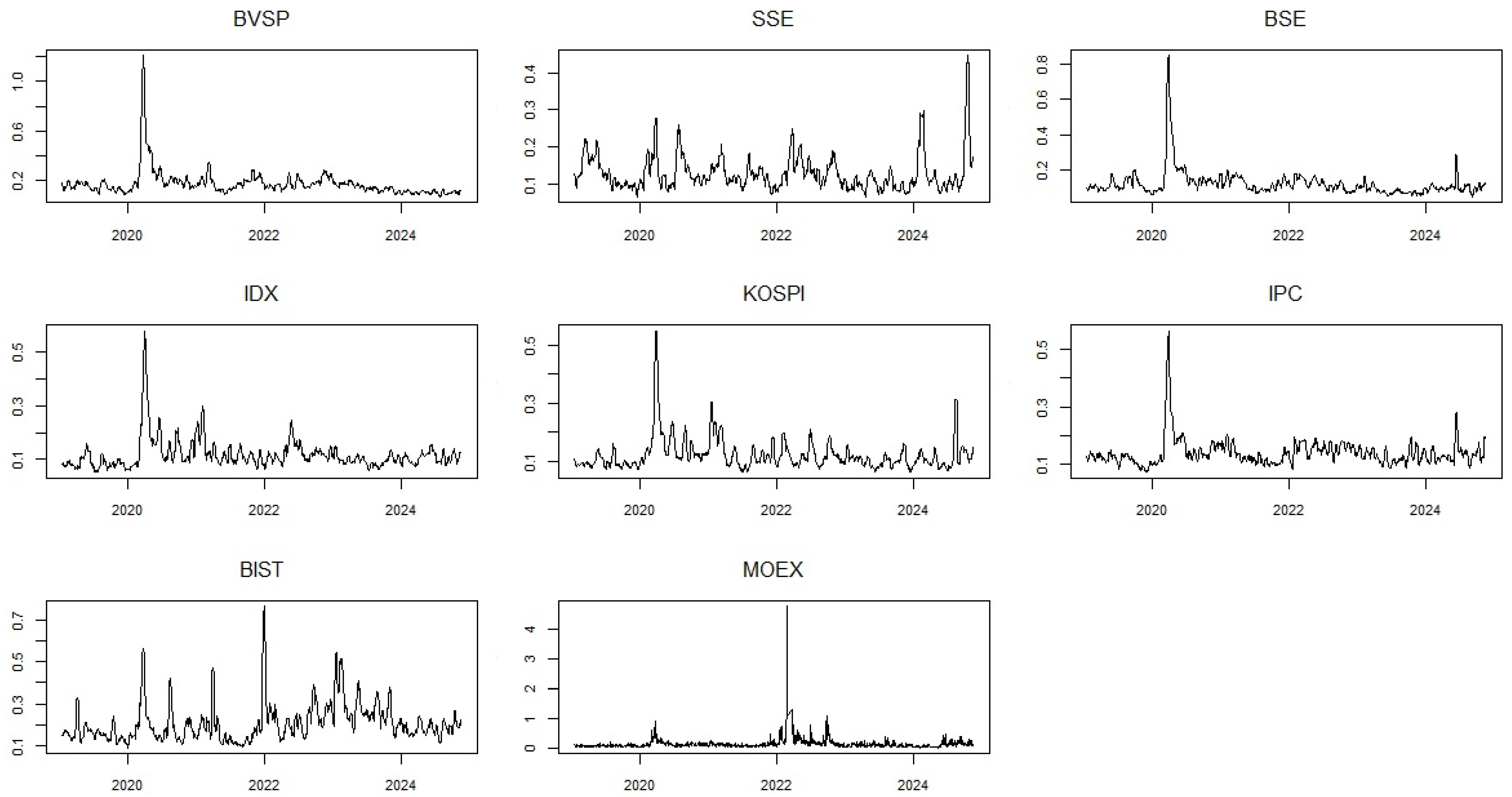
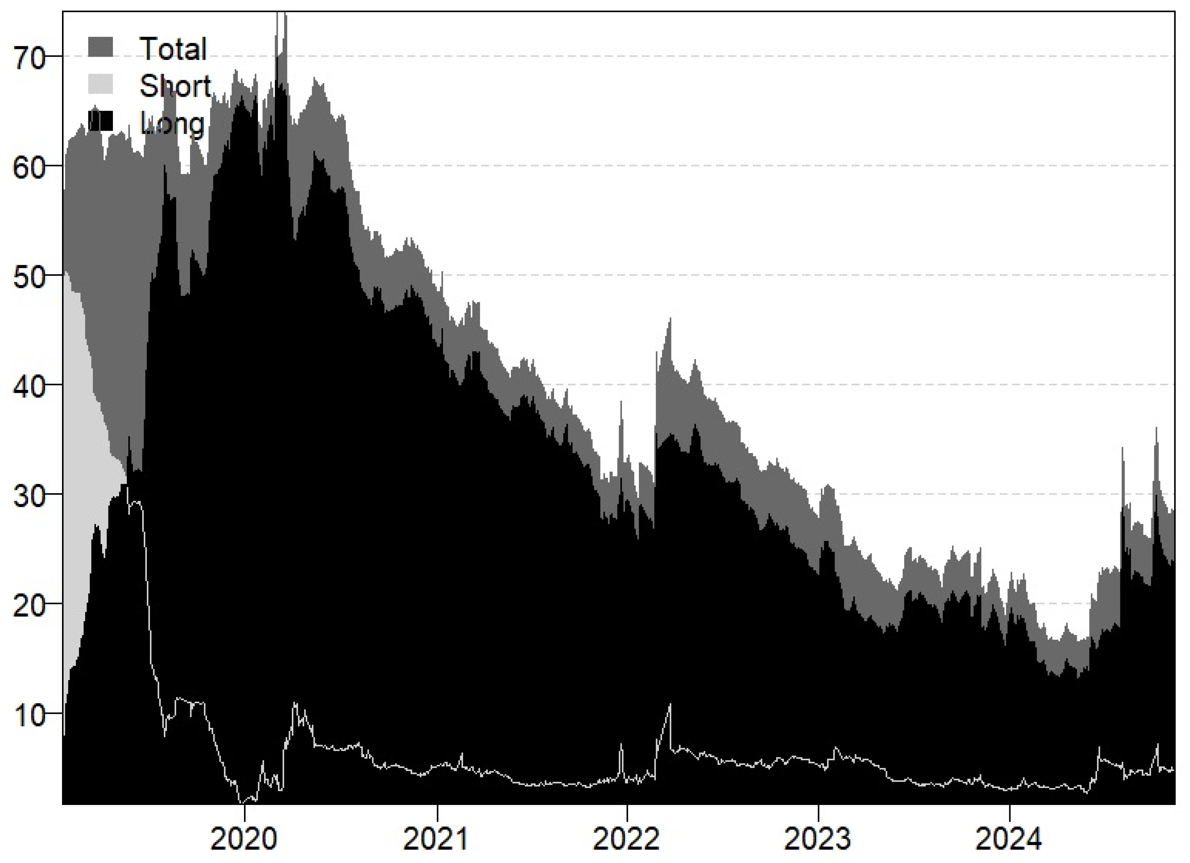

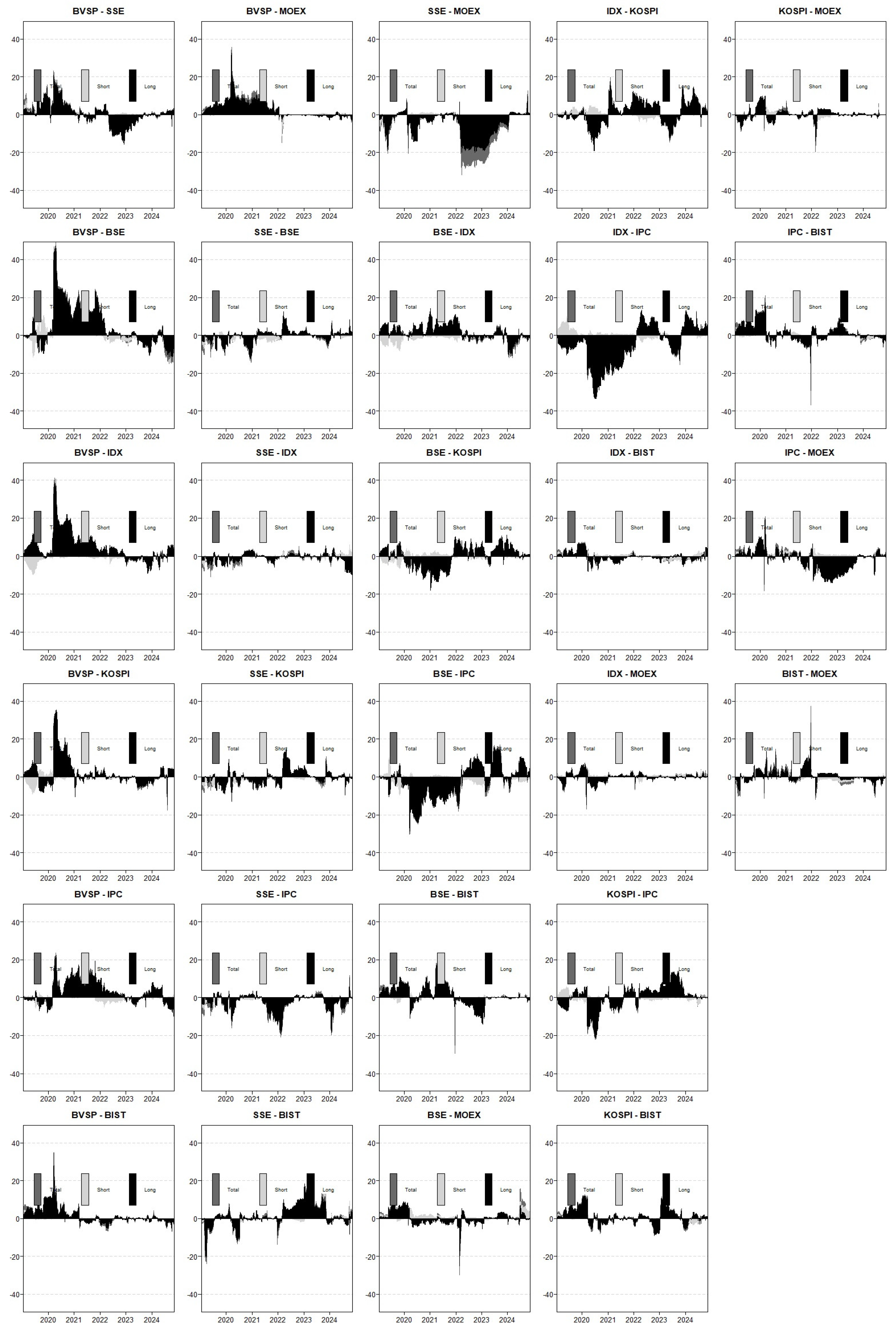

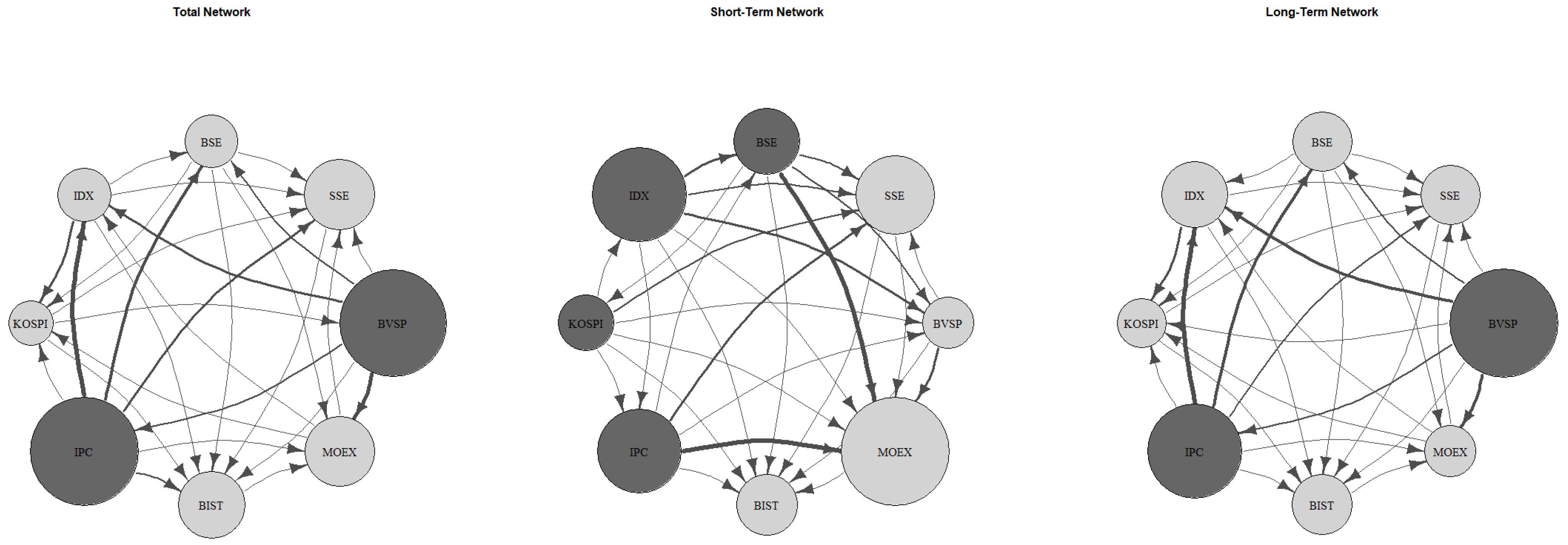
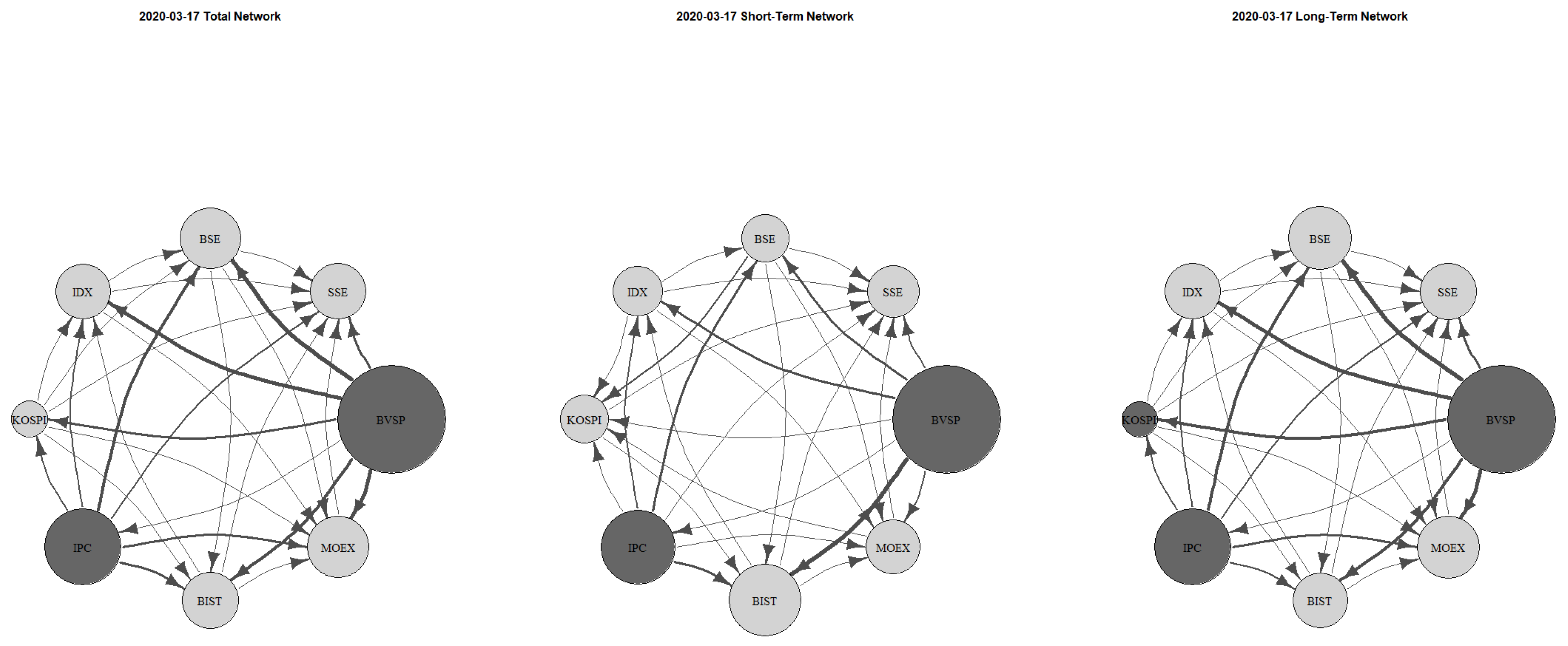
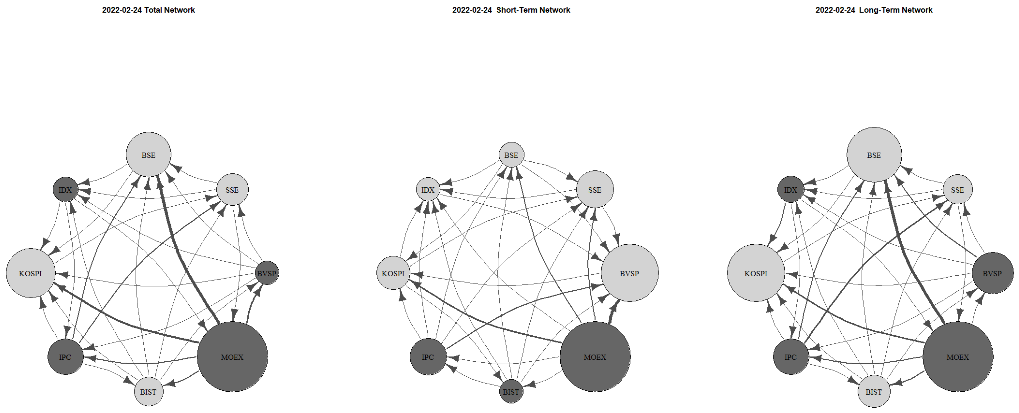
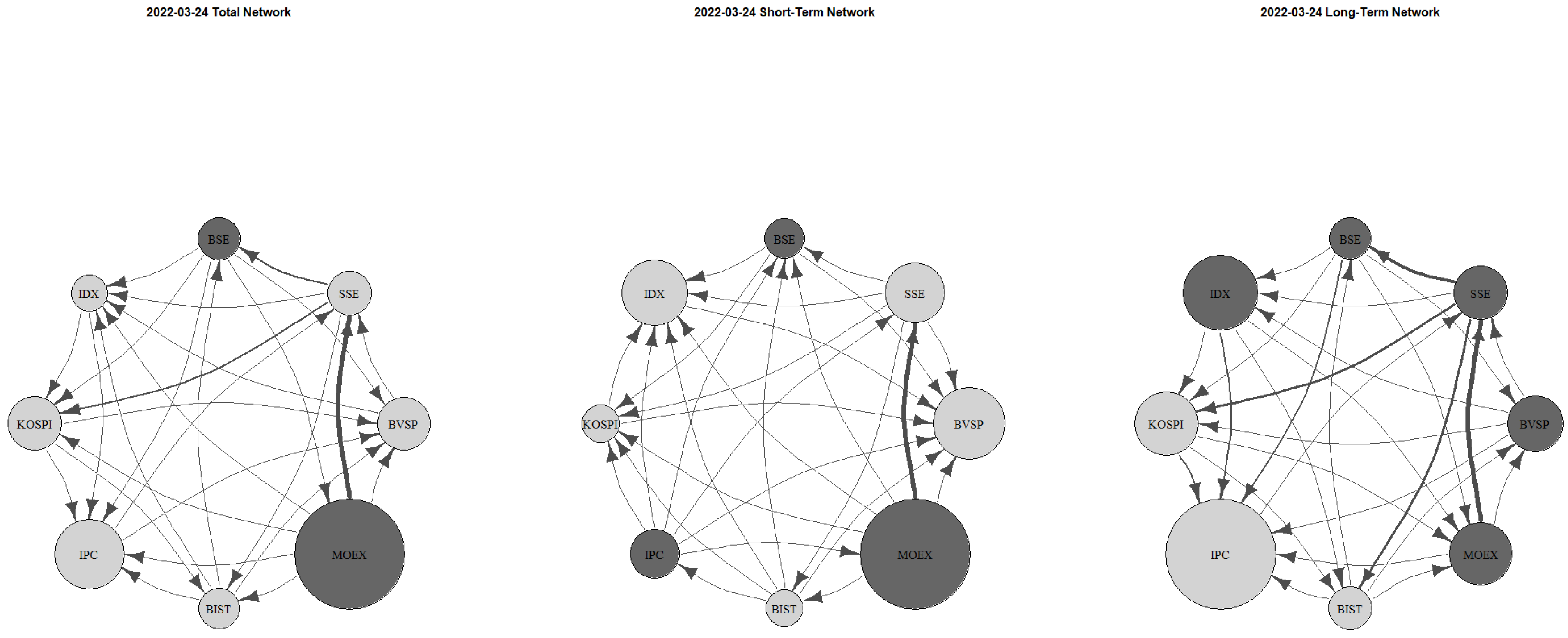
Disclaimer/Publisher’s Note: The statements, opinions and data contained in all publications are solely those of the individual author(s) and contributor(s) and not of MDPI and/or the editor(s). MDPI and/or the editor(s) disclaim responsibility for any injury to people or property resulting from any ideas, methods, instructions or products referred to in the content. |
© 2025 by the authors. Licensee MDPI, Basel, Switzerland. This article is an open access article distributed under the terms and conditions of the Creative Commons Attribution (CC BY) license (https://creativecommons.org/licenses/by/4.0/).