Granular Fuzzy Fractional Financial Systems Governed by Granular Caputo Fractional Derivative

Abstract

A granular fuzzy fractional financial system (GFFFS) is important for modeling real-world market uncertainties and complexities compared to conventional financial models. Unlike traditional approaches, a GFFFS offers enhanced precision in risk assessment, captures the long-term memory effects with the fractional derivatives, and effectively deals with the uncertainty and granularity in financial data through fuzzy logic. This model overcomes the limitations of the traditional model by accurately representing nonlinear dynamics, extreme volatility, and uncertain behavioral shifts in financial markets. The study of such models can be complex and challenging. However, developing an effective technique for solving such systems analytically and approximately is essential. This article aims to introduce and investigate a GFFFS using granular Caputo fractional derivatives. The behavior of the proposed model is studied using two distinct approaches, including an analytical approach, by applying the fuzzy Laplace transform technique and a numerical approach by employing fuzzy integral equations. Moreover, the existence and uniqueness of the extracted fuzzy solution are determined using the Banach contraction principle. To analyze the nonlinearity of the proposed model, the introduced numerical scheme is employed to illustrate the uncertain behavior of the proposed model graphically. This research provides deeper insights that can help decision-makers make better financial market decisions.

1. Introduction

All real-world scenarios are inherently based on uncertainty. There is often a need to develop a nonlinear model and solve and explain the fuzzy-based result one encounters in fuzziness. Generally, financial engineering domains are governed by partial and ordinary differential equations (PDEs/ODEs). These PDEs/ODEs generally depend upon complex environments. This complexity can be handled more precisely under fractional-order PDEs/ODEs. However, some parameters and variables of the DEs are considered to be crisp or well-defined. Instead of depicting specific values, the information about these parameters and variables may need to be more specific or complete due to errors in observations, measurements, or experiments. To handle such uncertainty, one can employ stochastic, statistical methods, or fuzzy set theory. However, stochastic and statistical methods deal with uncertainty arising from natural randomness in processes. In contrast, fuzzy set theory addresses uncertainty arising from a lack of knowledge or piece of information regarding model variables and parameters.

Fuzzy differential equations (FDEs) have been extensively used to study natural phenomena and have attracted considerable attention from researchers employing mathematical approaches and computer simulations. The term FDEs was first introduced in [1]. Significant research on FDEs has been conducted by determining the E&U of solutions, introducing new techniques, and analyzing their behavior to gain insights into the model [2,3]. Several approaches for dealing with FDEs include the fuzzy natural transform method, Zadeh’s extension principle, the fuzzy Laplace transform (FLT) method, fuzzy neural networks, and fuzzy differential inclusions. For more detailed information, see [4,5,6,7,8]. The closed-form analytical fuzzy solution of the generalized fractional Bagley–Torvik equation using gH-differentiability in uncertain environments was investigated in [9]. The authors extracted the solution using the FLT technique, represented in the Mittag-Leffler function (M-LF) form. These fuzzy derivatives derived from fuzzy standard interval arithmetic (FSIA) have certain limitations that restrict their applications. Some limitations are outlined as follows: (i) The analytical or numerical study of FDEs using fuzzy derivative under FSIA leads to the CPLV [10]. There are multiple extracted fuzzy solutions using FSIA. Moreover, every real-world problem follows the physical laws, and the behavior of phenomena can be predicted using FDEs. Various solutions are determined if the physical laws imposed on the mathematical model are violated. Therefore, a key drawback of fuzzy derivatives is that they suffer from CPLV. (ii) The existence of fuzzy derivatives under the FSIA framework is contingent upon the existence of the Hukuhara difference. If the H-difference does not exist, then the fuzzy derivatives also do not exist [11]. (iii) The FDEs using fuzzy derivatives in FSIA of n dimension are converted into $2n$ classical differential systems. This restriction poses challenges for the comprehensive analysis and investigation of FDEs. (iv) The fuzzy solutions of FDEs using fuzzy derivatives are not the same. This phenomenon is also known as the UBM phenomenon. (v) Fuzzy derivatives within the framework of FSIA often encounter challenges in factorization. (vi) FDEs in FSIA usually generate multiple or infinite solutions. These solutions add complexity to interpreting the results [12]. The novel idea of differentiability, generally known as the granular differentiability ($gr$-derivative), to analyze FDEs in new patterns was developed in [11]. This approach uniquely addressed the uncertainty of FDEs by using RDM-fuzzy interval arithmetic. The novel idea of this approach was to represent the horizontal membership function (HMF) of the fuzzy numbers (FNs) and the operations defined accordingly. This derivative was introduced to overcome and minimize the limitation of the fuzzy derivatives from FSIA. Granular FDEs allow us to determine the unique solution for the system, and hence, this technique is set apart from other methods. Some of the advantages of a granular derivative or granular differentiable (GRD) in the analysis of FDEs are outlined in the following: Fuzzy solution of FDEs using GRDs is simple and straightforward. FDEs with GRDs do not require the solution’s support over the domain of the FDE to be inherently monotonic. FDEs using GRDs effectively overcome and avoid the limitations of the solutions’ doubling property, diversity, and UBM phenomenon.

1.1. Motivation and Contribution

The financial system plays a vital role in facilitating economic growth [13,14,15]. This model makes it possible to allocate resources effectively and provide financial stability. Several researchers have introduced new methodologies and schemes to understand this system comprehensively [16,17,18]. The mathematical modeling of the financial system requires more precise, accurate, and reliable data. The complexities of this phenomenon are usually beyond one’s grasp. This complexity can significantly negatively impact stock exchanges, banks, markets, insurance companies, and other sectors [19,20]. Finance has been considered an essential field of research that offers knowledge of both academic and government policies. People without complete information about this system may have various queries. Mathematical models play a vital role in explaining and understanding the dynamic behavior of real-world problems. Shone [21] examined dynamic economic systems using phase diagrams. That analysis covered quantitative and qualitative dynamic systems such as linear and nonlinear systems, a system of equations models, and continuous and discrete dynamics. Chian et al. [22] examined the intricate dynamics of economic systems using a forced oscillator model. They demonstrated that these systems showed complex behaviors, including multistability, multiscale dynamics, and the coexistence of order and chaos. Wang et al. [23] studied the nonlinear time-delay fractional financial system. They used the approximation technique to solve the system and analyzed stability, including bifurcation behavior and periodic and chaotic states. Elouahab et al. [24] introduced and investigated the fractional financial system of chaos control. They used several control schemes to stabilize the chaotic behavior and navigate the system toward desired states. Johansyah et al. [25] proposed a fractional financial hyperchaos and control system with profit margin. They studied the dynamics of that model by incorporating the idea of profit margin. That study explored the hyperchaotic behavior of the system and determined several control techniques to stabilize the system. Olayiwola et al. [26] studied a fractional financial mathematical model. That model incorporated the maximum investment demand and minimum interest rate as control parameters. The study investigated how these characteristics affected complicated dynamics, bifurcation behavior, and system stability. Li et al. [27] developed a numerical scheme to solve fractional-order stochastic delay DEs. They used the spectral technique to extract the approximate solution and determined the comprehensive stability analysis to check the accuracy of the proposed method. Qayyum et al. [28] studied the analytical solution of a 4D fractional financial model using the He–Laplace algorithm. They explored the system’s dynamics, including chaotic behavior and optimal control techniques for system stability. Pakhira et al. [29] proposed a fractional economic order quantity (EOQ) model to discuss the instantaneous inventory level change by considering time-varying holding cost. Liu et al. [30] presented a new granular fuzzy fractional cobweb model. They provided a new technique for modeling and analyzing complex systems with memory effects. Xu et al. [31] constructed a robust control technique for fuzzy fractional Brownian motion. They determined the system’s stability and performance using the proposed method. Xu et al. [32] introduced a fuzzy finite-time tracking control technique for solving nonlinear systems. Ali et al. [33] analyzed the stability of stochastic fuzzy fractional BAM neural networks using time delays. They investigated the dynamic behavior of the proposed systems. Song et al. [34] developed a fuzzy output feedback control to solve the uncertain nonlinear fractional delay systems with input saturation. Xu et al. [35] studied the fractional financial risk system. They investigated the dynamics and synchronization using a synchronization projection scheme and determined the synchronization between identical or non-identical systems. Mesgarani et al. [36] introduced a new fuzzy approach to study the dynamics of financial systems. They used fuzzy logic to deal with the uncertainty in the evaluation process. Qayyum et al. [37] analyzed the fractional Wu–Zhang dynamical system in a fuzzy environment. They extracted the potential solution using the He–Mohand algorithm. Johansyah et al. [38] analyzed a hyperchaotic financial system, including sinusoidal hyperbolic nonlinearity. They determined the dynamic properties of the system, including hyperchaos and chaos. They also developed an adaptive fuzzy neural controller to assess the system’s stability. Qayyum et al. [39] analyzed the fuzzy fractional KDV system under Gaussian Caputo differentiability. They used the extended HM algorithm to extract the system’s analytical solutions. Qayyum et al. [40] investigated a fuzzy chaotic fractional financial system using the generalized He–Mohand technique. The system was incorporated under uncertain initial conditions (FICs) and fractional-order derivatives in the Caputo sense. Aderyani et al. [41] extracted the approximate solution of fuzzy fractional financial and Lorenz systems. They used the uncertain parameters and initial conditions to overcome and deal with the uncertainty of these systems. Bian and Li [42] developed a fuzzy novel approach to examine the price of European options using sub-fractional Brownian motion. That technique significantly dealt with the uncertainties of the model by incorporating fuzziness. Rehman et al. [43] studied a fractional financial system using Atangana–Baleanu Caputo (ABC) derivative. They developed an approximate technique to determine the system’s solution. That model involved three variables: I (interest rate), D (investment demand), and P (price index). The model also incorporated crisp parameters: a (saving amount), b (cost of investment), and c (demand elasticity). Alsenafi et al. [44] developed an explicit scheme to determine a geometric Asian power option with floating strike and transaction cost. They used a fractional geometric Brownian model with uncertain parameters. Nand [45] introduced an inventory control technique by incorporating fuzzy parameters for nonlinear demand influenced by factors including price, quality, and supply levels. The study also discussed granular differentiation for optimizing fuzzy production inventory systems. Brar et al. [46] analyzed a fractional-order returns-over-risk model. That model offered a comprehensive portfolio as compared to risk-minimization strategies. Xiong et al. [47] analyzed the efficiency of an uncertain Bayesian model for financial risk assessment. Babakordi et al. [48] developed a Laplace transform scheme to solve fuzzy fractional differential equations in uncertain environments. That study was also applied to economic price adjustment models to determine the uncertainty and vagueness of the model. Sukono et al. [49] discussed financial chaotic systems using fractional-order derivatives. The study showed that the fractional financial risk system exhibited periodic and chaotic behavior. Hashemi et al. [50] investigated an option pricing model using uncertain parameters and initial conditions with the Mittag-Leffler kernel. Rahaman et al. [51] developed a solution technique for the economic order quantity (EOQ) model using fuzzy logic and fractional-order derivatives. Their model generalized the classical EOQ by incorporating fuzzy logic and fractional calculus, with trapezoidal fuzzy numbers as parameters.

1.2. Fundamental Difference Between Fuzzy and Stochastic Modeling

Stochastic models incorporate randomness in the system, where variables follow probability distributions and require statistical data to estimate their parameters. In contrast, fuzzy models are designed to handle uncertainty and incomplete information. They are instrumental when exact probabilities are unknown or when financial data are qualitative—such as verbal estimates including high inflation, medium risk, or expert opinions. The fuzzy analysis is better suited for financial systems as it effectively captures vague, uncertain data and complex market behaviors. Unpredictable factors continually influence financial markets, including investor sentiment, policy changes, and macroeconomic trends. Fuzzy models excel in managing such uncertainty compared to stochastic models, as they employ human-like reasoning to interpret imprecise terms such as low risk or moderate inflation. Furthermore, financial systems often exhibit nonlinear and dynamic relationships between variables. When combined with fuzzy logic, fractional-order modeling can account for memory effects and hereditary properties, enabling a more comprehensive representation of these nonlinear patterns. In contrast, stochastic models typically rely on linear approximations, which may fail to capture real-world complexities fully. This makes fuzzy modeling a more robust and practical choice for financial analysis.

1.3. Model Formulation

Financial markets are inherently characterized by uncertainty from asset price volatility, lack of information, and irrational investor behavior. Traditional models often fail to capture these complexities, leading to significant discrepancies between theoretical predictions and real-world market dynamics. For instance, during crises (like the 2008 crash or COVID-19 market shocks), systems present nonlinear memory effects, ambiguity in granular data, and sudden regime shifts. The traditional integer-order models cannot adequately represent these accurately. Thus, fuzzy fractional approaches are crucial: non-integer-order derivatives encode long-term dependencies, while fuzzy logic quantifies the uncertainty and vagueness in market sentiment. The proposed model fills this gap by incorporating the granular Caputo-based fractional derivative in a fuzzy fractional financial system that rigorously accounts for such uncertainties. The proposed uncertain fractional financial model generalizes the classical fractional financial model by incorporating two key modern aspects: fractional calculus, which captures memory effects and hereditary properties in financial systems, and fuzzy uncertainty, which accounts for epistemic vagueness in the model’s parameters. We use three state variables in the model formulation: the interest rate ($\mathbb{I}$), the demand for investment ($\mathbb{D}$), and the price index ($\mathbb{P}$). The state variable ($\mathbb{I}$) in financial phenomena is affected by the difference between savings and investment and the cost of raw materials. The volatility of ($\mathbb{D}$) is proportional to investment and inversely proportional to the interest rate and investment cost. The difference between supply and demand in the trading market controls ($\mathbb{P}$), which is additionally influenced by the inflation rate. In our approach, the savings amount is denoted by $\mathfrak{a}$, the investment cost is denoted by $\mathfrak{b}$, and the demand elasticity in the business market is denoted by $\mathfrak{c}$. Based on these assumptions, the financial dynamics are modeled using the following ordinary differential equations:

$$\begin{array}{cc}\hfill {\displaystyle \frac{d\mathbb{I}}{dz}}& :=\mathbb{P}+\mathbb{I}\mathbb{D}-\mathfrak{a}\mathbb{I}.\hfill \end{array}$$

(1)

The interest rate in Equation (1) depends on fluctuations in both the price index ($\mathbb{P}$) and investment demand ($\mathbb{D}$). The term $(\mathbb{D}-\mathfrak{a})\mathbb{I}$ indicates that while increased investment demand ($\mathbb{D}$) raises the interest rate ($\mathbb{I}$), this effect is counterbalanced by higher savings ($\mathfrak{a}$).

$$\begin{array}{cc}\hfill {\displaystyle \frac{d\mathbb{D}}{dz}}& :=1-\mathfrak{b}\mathbb{D}-{\mathbb{I}}^2.\hfill \end{array}$$

(2)

Equation (2) describes investment demand dynamics. The constant 1 represents exogenous factors. The term $-\mathfrak{b}\mathbb{D}$ reflects reduced demand due to higher investment costs. The term $-{\mathbb{I}}^2$ captures how elevated interest rates discourage investment.

$$\begin{array}{cc}\hfill {\displaystyle \frac{d\mathbb{P}}{dz}}& :=-\mathbb{I}-\mathfrak{c}\mathbb{P}.\hfill \end{array}$$

(3)

In Equation (3), the term $-\mathbb{I}$ shows that higher interest rates lower the price index by reducing purchasing power. The term $-\mathfrak{c}\mathbb{P}$ models inflation’s natural stabilization over time. Financial systems exhibit complex non-local behavior with memory effects, making fractional derivatives with singular kernels essential for accurate modeling. This work introduces the granular Caputo fractional derivative ($gr$-CFD) to represent financial dynamics and fuzzy dynamic systems to handle parameter vagueness and incomplete information. These approaches provide realistic representations of uncertain financial behaviors, offer extensibility to other economic models, and align closely with real-world financial phenomena. The following granular fuzzy fractional differential system models the complete uncertain dynamics:

$$\left\{\begin{array}{c}{}_{0^{+}}{}^{gr}\mathcal{D}^{\vartheta }\mathbb{I}:=\mathbb{P}+\mathbb{I}\mathbb{D}-\mathfrak{a}\mathbb{I},\hfill \\ {}_{0^{+}}{}^{gr}\mathcal{D}^{\vartheta }\mathbb{D}:=1-\mathfrak{b}\mathbb{D}-{\mathbb{I}}^2,\hfill \\ {}_{0^{+}}{}^{gr}\mathcal{D}^{\vartheta }\mathbb{P}:=-\mathbb{I}-\mathfrak{c}\mathbb{P},\hfill \end{array}\right.$$

(4)

with fuzzy initial conditions (FICs)

$$\begin{array}{c}\hfill \mathbb{I}\left(0\right):={\mathbb{I}}_0,\mathbb{D}\left(0\right):={\mathbb{D}}_0\mathrm{and}\mathbb{P}\left(0\right):={\mathbb{P}}_0,\end{array}$$

(5)

where ${}_{0^{+}}{}^{gr}\mathcal{D}^{\vartheta }$ is the $gr$-CFD of order $\vartheta$ with respect to the state vectors $\mathbb{I}$, $\mathbb{D}$, and $\mathbb{P}$. Moreover, $\mathbb{I}:[0,T]\times {\mathrm{\Xi }}_{\mathcal{R}}⟶{\mathrm{\Xi }}_{\mathcal{R}}$, $\mathbb{D}:[0,T]\times {\mathrm{\Xi }}_{\mathcal{R}}⟶{\mathrm{\Xi }}_{\mathcal{R}}$, and $\mathbb{P}:[0,T]\times {\mathrm{\Xi }}_{\mathcal{R}}⟶{\mathrm{\Xi }}_{\mathcal{R}}$ are continuous fuzzy-valued functions and $\mathfrak{a},\mathfrak{b},\mathfrak{c}\in {\mathrm{\Xi }}_{\mathcal{R}}$. The contribution of the proposed work is outlined as follows: This article introduces and investigates the GFFFS using the $gr$-CFD. The behavior of the proposed model is studied using two distinct techniques, including the analytical scheme by applying the FLT technique and the introduced numerical technique using fuzzy integral equations (FIEs). The existence and uniqueness (E&U) of the proposed fuzzy solutions are determined. To enhance the originality of this research, the introduced numerical scheme is employed to graphically illustrate the uncertain dynamics of the proposed fractional financial model.

The remainder of the article is structured as follows: Section 2 introduces fundamental concepts and terminologies related to the granular representation of FN, the granular fractional integral ($gr$-FI), and the $gr$-CFD. The E&U of the mild solution for the GFFFS under the $gr$-CFD are presented in Section 3. The numerical solution of the GFFFS is extracted in Section 4. Section 5 provides concluding remarks and future directions.

2. Basic Concepts

This section addresses the fundamental concept of fuzzy analysis and its granular representations.

A triangular fuzzy number [1] (TFN) $\mathfrak{m}$ is a fuzzy subset of real numbers characterized by the three real numbers ${\mathfrak{m}}_1$, ${\mathfrak{m}}_2$, and ${\mathfrak{m}}_3$, where ${\mathfrak{m}}_1\le {\mathfrak{m}}_2\le {\mathfrak{m}}_3$. The membership function ${\mu }_{\mathfrak{m}}\left(z\right)$ defines the degree to which an element z belong to $\mathfrak{m}$ and is defined as:

$${\mu }_{\mathfrak{m}}\left(z\right)=\left\{\begin{array}{cc}0\hfill & \mathrm{if}z<{\mathfrak{m}}_1,\hfill \\ {\displaystyle \frac{z-{\mathfrak{m}}_1}{{\mathfrak{m}}_2-{\mathfrak{m}}_1}}\hfill & \mathrm{if}{\mathfrak{m}}_1\le z<{\mathfrak{m}}_2,\hfill \\ 1\hfill & \mathrm{if}z={\mathfrak{m}}_2,\hfill \\ {\displaystyle \frac{{\mathfrak{m}}_3-z}{{\mathfrak{m}}_3-{\mathfrak{m}}_2}}\hfill & \mathrm{if}{\mathfrak{m}}_2<z\le {\mathfrak{m}}_3,\hfill \\ 0\hfill & \mathrm{if}z>{\mathfrak{m}}_3.\hfill \end{array}\right.$$

The $\alpha$-cut of $\mathfrak{m}$, denoted by ${\left[\mathfrak{m}\right]}^{\alpha }$, is a crisp set containing all elements with its membership degree at least $\alpha$. For a TFN, it is given by the following closed interval

$$\begin{array}{c}\hfill {\left[\mathfrak{m}\right]}^{\alpha }=[{\mathfrak{m}}_1+\alpha ({\mathfrak{m}}_2-{\mathfrak{m}}_1),{\mathfrak{m}}_3-\alpha ({\mathfrak{m}}_3-{\mathfrak{m}}_2)].\end{array}$$

(6)

Let ${\mathrm{\Xi }}_{\mathcal{R}}$ be the collection of FN [52] $\mathfrak{m}:[a,b]\subseteq \mathbb{R}⟶\mathbb{I}:=[0,1]$, such that it adheres to the given properties: (i) Normality—There is a $z\in \mathbb{R}$ for which $\mathfrak{m}=1$. (ii) Upper semi-continuous—The inequality $\underset{z\to z_0^{\pm }}{lim}\mathfrak{m}\left(z\right)\le \mathfrak{m}\left(z_0\right)$ holds for every $z_0\in \mathbb{R}$; (iii) Compact support—$\overline{\mathrm{supp}\left(\mathfrak{m}\right)}=\mathrm{cl}\{z\in \mathbb{R}:\mathfrak{m}\left(z\right)\ge \alpha \}$ is compact; (iv) Fuzzy convex—For every $\lambda \in \mathbb{I}$ and $z,y\in \mathbb{R}$ the following inequality $\mathfrak{m}(\lambda z+(1-\lambda \left)y\right)\ge min\left\{\mathfrak{m}\right(z),\mathfrak{m}(y\left)\right\}$ holds. The $\alpha$-level values of $\mathfrak{m}$ are ${\left[\mathfrak{m}\right]}^{\alpha }=\{z\in \mathbb{R}\mid \mathfrak{m}\left(z\right)\ge \alpha ,\mathrm{if}0<\alpha \le 1\}$. The support of $\mathfrak{m}$, ${\left[\mathfrak{m}\right]}^0$, is the classical set of every $z\in \mathbb{R}$ such that $\mathfrak{m}\left(z\right)>0$, i.e., ${\left[\mathfrak{m}\right]}^0=\{z\in \mathbb{R}:\mathfrak{m}\left(z\right)>0\}$. The $\alpha$-level set ${\left[\mathfrak{m}\right]}^{\alpha }$ of $\mathfrak{m}$ constitutes a non-empty, compact, and fuzzy convex subset of $\mathbb{R}$. Moreover, ${\left[\mathfrak{m}\right]}^{\alpha }$ can be expressed as a closed interval, written as ${\left[\mathfrak{m}\right]}^{\alpha }=[{\mathfrak{m}}_{\alpha }^{-},{\mathfrak{m}}_{\alpha }^{+}]$, for any $0\le \alpha \le 1$. Furthermore, Bede and Stefanini [52] introduced all the operations and properties of the class of FNs using $\alpha$-cuts. All this analysis is conducted using vertical membership. However, using vertical membership in FNs leads to various complexities, resulting in computational inconsistencies within fuzzy arithmetic. Piegat and Landowski [53] addressed this issue and introduced the concepts of HMFs to overcome the hurdles of vertical membership. Suppose $\mathfrak{m}:[a,b]\subseteq \mathbb{R}⟶\mathbb{I}$ is an FN. The granular representation [11] of FN $\mathfrak{m}$ is defined as ${\mathfrak{m}}^{\mathrm{gr}}:\mathbb{I}\times \mathbb{I}⟶[a,b]$, where $(\alpha ,\pi )\mapsto {\mathfrak{m}}^{\mathrm{gr}}(\alpha ,\pi )={\mathfrak{m}}_{\alpha }^{-}+\mathrm{len}\left({\left[\mathfrak{m}\right]}^{\alpha }\right)\pi$. In this context, gr represents the granular form of $\mathfrak{m}$ within the interval $x\in [a,b]$, where $\alpha \in \mathbb{I}$ and $\pi \in \mathbb{I}$. The HMF of $\mathfrak{m}\in {\mathrm{\Xi }}_{\mathcal{R}}$, denoted by $\mathbb{H}\left(\mathfrak{m}\right)$, is defined as $\mathbb{H}\left(\mathfrak{m}\right)\triangleq {\mathfrak{m}}^{\mathrm{gr}}(\alpha ,\pi )$. A series of $\alpha$ values and cover variable $\pi$ characterize an FN under the HMF. The variation in the cover variable $\pi$ spans the entire range of ${\left[\mathfrak{m}\right]}^{\alpha }$ when the $\alpha$ value is fixed. Similarly, if the cover variable $\pi$ is held constant, the variation in $\alpha$ values yields specific crisp numbers from the cover values. Next, we address the reconstruction of the $\alpha$-level sets of the FN $\mathfrak{m}$ [11] from the granular representation $\mathbb{H}\left(\mathfrak{m}\right)$ by applying the following formula

$$\begin{array}{c}\hfill {\mathbb{H}}^{-1}\left({\mathfrak{m}}^{gr}(\alpha ,\pi )\right):={\left[\mathfrak{m}\right]}^{\alpha }:=\left[\underset{\nu \ge \alpha }{inf}\underset{\pi }{min}{\mathfrak{m}}^{gr}(\nu ,\pi ),\underset{\nu \ge \alpha }{sup}\underset{\pi }{max}{\mathfrak{m}}^{gr}(\nu ,\pi )\right].\end{array}$$

(7)

Now, we discuss the arithmetic operations on the class of FN ${\mathrm{\Xi }}_{\mathcal{R}}$ as follows: Let ${\mathfrak{m}}_1$ and ${\mathfrak{m}}_2$ be the two FNs with their corresponding HMFs denoted by $\mathbb{H}\left({\mathfrak{m}}_1\right)$ and $\mathbb{H}\left({\mathfrak{m}}_2\right)$, respectively. We define the following operations: (i) addition: $\mathbb{H}({\mathfrak{m}}_1\oplus {\mathfrak{m}}_2)=\mathbb{H}\left({\mathfrak{m}}_1\right)+\mathbb{H}\left({\mathfrak{m}}_2\right)$; (ii) subtraction: $\mathbb{H}\left({\mathfrak{m}}_1{\ominus }^{gr}{\mathfrak{m}}_2\right)=\mathbb{H}\left({\mathfrak{m}}_1\right)-\mathbb{H}\left({\mathfrak{m}}_2\right)$; (iii) multiplication: $\mathbb{H}\left({\mathfrak{m}}_1{·}^{gr}{\mathfrak{m}}_2\right)=\mathbb{H}\left({\mathfrak{m}}_1\right)\times \mathbb{H}\left({\mathfrak{m}}_2\right)$; (iv) division: $\mathbb{H}\left({\mathfrak{m}}_1{÷}^{gr}{\mathfrak{m}}_2\right)={\displaystyle \frac{\mathbb{H}\left({\mathfrak{m}}_1\right)}{\mathbb{H}\left({\mathfrak{m}}_2\right)}}$, where $\mathbb{H}\left({\mathfrak{m}}_2\right)\ne 0$ and $\alpha ,\pi \in \mathbb{I}$. The set ${\mathrm{\Xi }}_{\mathcal{R}}$, equipped with the arithmetic operations, constitutes a vector space. Now, we define the concept of fuzzy-valued function (FVF) [11]. An FVF $\varkappa$ is characterized as a function $\varkappa :[a,b]\to {\mathrm{\Xi }}_{\mathcal{R}}$. Furthermore, suppose that $\varkappa \left(z\right)$ has n distinct FNs ${\mathfrak{m}}_1,{\mathfrak{m}}_2,\dots ,{\mathfrak{m}}_n$. The HMF is denoted by $\mathbb{H}\left(\varkappa \left(z\right)\right)\triangleq {\varkappa }^{\mathrm{gr}}(z,\alpha ,\pi )$, defined by the following mapping:

$$\begin{array}{c}\hfill {\varkappa }^{\mathrm{gr}}:[a,b]\times \mathbb{I}\times \underset{n\mathrm{times}}{\underbrace{\mathbb{I}\times \dots \times \mathbb{I}}}\to \mathbb{R},\mathrm{where}\alpha \in \mathbb{I}\mathrm{and}\pi \triangleq ({\pi }_1,{\pi }_2,\dots ,{\pi }_n).\end{array}$$

(8)

Following this, we define the granular metric as a mapping ${\rho }^{\mathrm{gr}}:{\mathrm{\Xi }}_{\mathcal{R}}\times {\mathrm{\Xi }}_{\mathcal{R}}\to {\mathbb{R}}^{+}\cup \left\{0\right\}$, such that

$${\rho }^{\mathrm{gr}}({\mathfrak{m}}_1,{\mathfrak{m}}_2)=\underset{\begin{array}{c}\alpha \end{array}}{sup}\underset{\begin{array}{c}\pi \end{array}}{max}\left|{\mathfrak{m}}_1^{\mathrm{gr}}(\alpha ,\pi )-{\mathfrak{m}}_2^{\mathrm{gr}}(\alpha ,\pi )\right|.$$

(9)

The space ${\mathrm{\Xi }}_{\mathcal{R}}$ endowed with the metric defined in (9) is a complete metric space (CMS). Moreover, it as a Banach space with the norm ${\parallel x\parallel }_1={\rho }^{\mathrm{gr}}({\mathfrak{m}}_1,\widehat{0})$. Now, we discuss some properties of the granular metric [54]. Suppose ${\mathfrak{m}}_1,{\mathfrak{m}}_2,{\mathfrak{m}}_3\in {\mathrm{\Xi }}_{\mathcal{R}}$, and $\lambda$ is a constant. In this case, the following claims hold: (i) ${\rho }^{\mathrm{gr}}({\mathfrak{m}}_1+{\mathfrak{m}}_3,{\mathfrak{m}}_2+{\mathfrak{m}}_3)={\rho }^{\mathrm{gr}}({\mathfrak{m}}_1,{\mathfrak{m}}_2)$. (ii) ${\rho }^{\mathrm{gr}}(\lambda {\mathfrak{m}}_1,\lambda {\mathfrak{m}}_2)=\left|\lambda \right|{\rho }^{\mathrm{gr}}({\mathfrak{m}}_1,{\mathfrak{m}}_2)$. (iii) ${\rho }^{\mathrm{gr}}({\mathfrak{m}}_1{\ominus }^{\mathrm{gr}}{\mathfrak{m}}_2,\widehat{0})={\rho }^{\mathrm{gr}}({\mathfrak{m}}_1,{\mathfrak{m}}_2)$. Consider ${\mathrm{\Xi }}_{\mathbb{R}}^n=\underset{n-times}{\underbrace{{\mathrm{\Xi }}_{\mathcal{R}}\times {\mathrm{\Xi }}_{\mathcal{R}}\times \cdots \times {\mathrm{\Xi }}_{\mathcal{R}}}}$. The metric on ${\mathrm{\Xi }}_{\mathbb{R}}^n$ is represented by ${\mathcal{D}}^{gr}$ and can be described by ${\mathcal{D}}^{gr}(\mathfrak{m},\mathfrak{n})={\sum }_{i=1}^n{\rho }^{gr}({\mathfrak{m}}_i,{\mathfrak{n}}_i)$, for every ${\mathfrak{m}}_i,{\mathfrak{n}}_i\in {\mathrm{\Xi }}_{\mathbb{R}}^n$, $i=1,2,3,\cdots ,n$. The set $({\mathrm{\Xi }}_{\mathbb{R}}^n,{\mathcal{D}}^{gr})$ is a CMS [55] and hence is a Banach space with norm $\parallel \mathfrak{m}\parallel ={\mathcal{D}}^{gr}(\mathfrak{m},\overline{0})$, where $\overline{0}=(\widehat{0},\widehat{0},\cdots ,\widehat{0})$ denotes the zero fuzzy vector.

Definition 1 

([11]). A FVF ϰ is said to be GRD at a fixed point $z_0\in (a,b)$, if the limit ${lim}_{h\to 0}{\displaystyle \frac{\varkappa (z_0+h){\ominus }^{\mathrm{gr}}\varkappa \left(z_0\right)}{h}}$ exists and is denoted by ${\varkappa }_{gr}^{\prime }\left(z_0\right)\in {\mathrm{\Xi }}_{\mathcal{R}}$. The FVF ${\varkappa }_{gr}^{\prime }\left(z_0\right)$ is also called the GRD of ϰ at $z_0$. The FVF ϰ is considered GRD if and only if ${\varkappa }_{gr}^{\prime }\left(z\right)$ exists for every $z\in (a,b)$. Denote ${\mathbb{C}}^1((a,b),{\mathrm{\Xi }}_{\mathcal{R}})$ the class of all continuously GRD functions on $(a,b)$. Moreover, an FVF ϰ is termed GRD if its HMF is differentiable. Moreover, we also have $\mathbb{H}\left({\varkappa }_{gr}^{\prime }\left(z_0\right)\right)={\displaystyle \frac{\partial {\varkappa }^{gr}(z_0,\alpha ,{\mu }_{\varkappa })}{\partial z}}$. Denote $L^1([a,b],\mathbb{R})$; then, ${}_{a^{+}}{}^C\mathcal{D}^{\vartheta }$ is the collection of all Lebesgue integrable continuous real-valued functions on the closed interval $[a,b]$.

Definition 2. 

The fractional integral ${\mathcal{I}}_{a^{+}}^{\vartheta }$ of order $\vartheta >0$ of $\varkappa \in L^1([a,b],\mathbb{R})$ is defined by

$$\begin{array}{c}\hfill {\mathcal{I}}_{a^{+}}^{\vartheta }\varkappa \left(z\right):={\displaystyle \frac{1}{\mathrm{\Gamma }\left(\vartheta \right)}}{\int }_a^z{\displaystyle \frac{\varkappa \left(p\right)}{{(z-p)}^{-\vartheta +1}}}dp,\end{array}$$

(10)

where $\mathrm{\Gamma }\left(\vartheta \right)={\int }_0^{\infty }{z}^{\vartheta -1}{e}^{-z}dz$.

Definition 3. 

The Caputo fractional derivative ${}_{a^{+}}{}^C\mathcal{D}^{\vartheta }$ of order $\vartheta >0$ of $\varkappa \in C^1([a,b],\mathbb{R})$ is defined by

$$\begin{array}{c}\hfill {}_{a^{+}}{}^C\mathcal{D}^{\vartheta }\varkappa \left(z\right):={\displaystyle \frac{1}{\mathrm{\Gamma }(n-\vartheta )}}{\int }_a^z{(z-p)}^{n-\vartheta -1}{\varkappa }^{\left(n\right)}\left(p\right)dp,\end{array}$$

(11)

where n is the natural number such that $n-1<\vartheta <n$ and $z\in [a,b]$.

Now, we present the notions of $gr$-FI and $gr$-CFD of FVFs, as discussed by Najariyan et al. [56].

Definition 4 

([56]). Let $\varkappa :[a,b]\subset \mathbb{R}⟶{\mathrm{\Xi }}_{\mathbb{R}}$. Then, the $gr$-FIs ${}^{gr}\mathcal{I}_{a^{+}}^{\vartheta }$ of order $\vartheta \in (0,1]$ of the FVF ϰ is defined by

$$\begin{array}{c}\hfill {}^{gr}\mathcal{I}_{a^{+}}^{\vartheta }\varkappa \left(z\right)={\displaystyle \frac{1}{\mathrm{\Gamma }\left(\vartheta \right)}}{\int }_a^z{(z-p)}^{\vartheta -1}\varkappa \left(p\right)dp.\end{array}$$

(12)

Remark 1. 

The HMF of the $gr$-FI ${}^{gr}\mathcal{I}_{a^{+}}^{\vartheta }\varkappa \left(z\right)$ defined in Definition 4 can be defined in the following manner

$$\begin{array}{cc}\hfill \mathbb{H}\left({}^{gr}\mathcal{I}_{a^{+}}^{\vartheta }\varkappa \left(z\right)\right)& ={\displaystyle \frac{1}{\mathrm{\Gamma }\left(\vartheta \right)}}{\int }_a^z\mathbb{H}\left({(z-p)}^{\vartheta -1}\varkappa \left(p\right)\right)dp,\hfill \\ \hfill & ={\displaystyle \frac{1}{\mathrm{\Gamma }\left(\vartheta \right)}}{\int }_a^z{(z-p)}^{\vartheta -1}\mathbb{H}\left(\varkappa \left(p\right)\right)dp={\mathcal{I}}_{a^{+}}^{\vartheta }\mathbb{H}\left(\varkappa \left(z\right)\right).\hfill \end{array}$$

(13)

Definition 5 

([56]). The $gr$-CFD ${}^{gr}\mathcal{D}_{a^{+}}^{\vartheta }\varkappa \left(z\right)$ of order $\vartheta \in (0,1]$ for the FVF ϰ is defined by

$$\begin{array}{c}\hfill {}_{a^{+}}{}^{gr}\mathcal{D}^{\vartheta }\varkappa \left(z\right)={\displaystyle \frac{1}{\mathrm{\Gamma }(1-\vartheta )}}{\int }_a^z{(z-p)}^{-\vartheta }{\varkappa }_{gr}^{\prime }\left(p\right)dp={}^{gr}\mathcal{I}_{a^{+}}^{1-\vartheta }\left({\varkappa }_{gr}^{\prime }\left(z\right)\right).\end{array}$$

(14)

Remark 2. 

Using analogous reasoning as in Remark 1, we can similarly infer that

$$\begin{array}{cc}\hfill \mathbb{H}\left({}_{a^{+}}{}^{gr}\mathcal{D}^{\vartheta }\varkappa \left(z\right)\right)& ={}_{a^{+}}{}^C\mathcal{D}^{\vartheta }\mathbb{H}\left(\varkappa \left(z\right)\right).\hfill \end{array}$$

(15)

Granular Laplace Transform for FVFs

First, we recall some basic concepts and terminology of the Laplace transform (LT). Then, we introduce the granular LT of an FVF and its HMF.

Definition 6. 

Suppose ϰ is the real-valued function such that its LT is denoted by $\mathcal{L}\left[\varkappa \left(z\right)\right]$, defined by

$$\begin{array}{c}\hfill \mathcal{L}\left[\varkappa \left(z\right)\right]={\int }_0^{\infty }{e}^{-pz}\varkappa \left(z\right)dz,\end{array}$$

(16)

for every $p\in \mathbb{C}$ such that the integral given in Equation (16) converges.

Theorem 1. 

Let ϰ and ψ be piecewise continuous functions of exponential order over $[0,T]$. The convolution of ϰ and $\mathfrak{y}$, denoted by $\varkappa \ast \mathfrak{y}$, is defined by

$$\begin{array}{c}\hfill (\varkappa \ast \mathfrak{y})\left(z\right)={\int }_0^z\varkappa \left(\tau \right)\mathfrak{y}(z-\tau )d\tau .\end{array}$$

(17)

By the convolution theorem, the Laplace transform of the convolution satisfies the property

$$\begin{array}{c}\hfill \mathcal{L}\left[(\varkappa \ast \mathfrak{y})\left(z\right)\right]=\mathcal{L}\left[\varkappa \left(z\right)\right]\mathcal{L}\left[\mathfrak{y}\left(z\right)\right].\end{array}$$

(18)

Remark 3. 

For every $0<\vartheta <1$, we have

$$\begin{array}{c}\hfill \mathcal{L}\left[{}_{a^{+}}{}^C\mathcal{D}^{\vartheta }\varkappa \left(z\right)\right]=p^{\vartheta }\mathcal{L}\left[\varkappa \left(z\right)\right]-p^{\vartheta -1}\varkappa \left(0\right).\end{array}$$

(19)

Now, we give the definition of the granular LT of an FVF in the following:

Definition 7 

([7]). Suppose $\varkappa \left(z\right)$ is a continuous FVF. The granular FLT is denoted by $\mathfrak{L}\left[\varkappa \left(z\right)\right]$ and is defined by:

$$\begin{array}{c}\hfill \mathfrak{L}\left[\varkappa \left(z\right)\right]={\int }_0^{\infty }{e}^{-pz}\varkappa \left(z\right)dz,\end{array}$$

(20)

if it exists, where $p>0$ is an integer.

Remark 4. 

The HMF of Definition 7 satisfies the following:

$$\begin{array}{cc}\hfill \mathbb{H}\left[\mathfrak{L}\left[\varkappa \left(z\right)\right]\right]& =:{\int }_0^{\infty }\mathbb{H}\left(e^{-pz}\varkappa \left(z\right)\right)dz,\hfill \\ \hfill & ={\int }_0^{\infty }{e}^{-pz}\mathbb{H}\left(\varkappa \left(z\right)\right)dz,\hfill \\ \hfill & =\mathcal{L}\left[\mathbb{H}\right(\varkappa \left(z\right)\left)\right].\hfill \end{array}$$

(21)

3. The Existence and Uniqueness of the Fuzzy Solution to the GFFFS Under $\mathit{g}\mathit{r}$-CFD

Now, we analyze the E&U of a mild solution of the following fuzzy initial value problem to the GFFFS under the $gr$-CFD

$$\left\{\begin{array}{cc}{}_{0^{+}}{}^{gr}\mathcal{D}^{\vartheta }\varkappa \left(z\right)\hfill & :=\mathrm{\Psi }(z,\varkappa (z\left)\right),z\in [0,T],\hfill \\ \varkappa \left(0\right)\hfill & :={\varkappa }_0,\hfill \end{array}\right.$$

(22)

where ${}_{0^{+}}{}^{gr}\mathcal{D}^{\vartheta }\varkappa \left(z\right)$ is the granular Caputo fractional derivative of FVF $\varkappa \left(z\right)$ of order $\vartheta \in (0,1]$, the uncertain initial condition ${\varkappa }_0\in C([0,T],{\mathrm{\Xi }}_{\mathbb{R}}^n)$, and $\mathrm{\Psi }:[0,T]\times {\mathrm{\Xi }}_{\mathbb{R}}^n⟶{\mathrm{\Xi }}_{\mathbb{R}}^n$ is a fuzzy-vector-valued function. Furthermore, $\mathrm{\Psi }(z,\varkappa (z\left)\right)$ is the sum of the linear and nonlinear terms of the proposed system. The solvability of the system (22) is determined under the following assumptions:

(HF − I) 

The functions $\mathrm{\Psi }(.,\varkappa ):[0,T]⟶{\mathrm{\Xi }}_{\mathbb{R}}^n$ and $\mathrm{\Psi }(z,.):{\mathrm{\Xi }}_{\mathbb{R}}^n⟶{\mathrm{\Xi }}_{\mathbb{R}}^n$ are measurable and continuous for each $\varkappa \in {\mathrm{\Xi }}_{\mathbb{R}}^n,z\in [0,T]$, respectively.

(HF − II) 

There exists $C_1$ such that ${\mathcal{D}}^{gr}(\mathrm{\Psi }(z,{\varkappa }_1),\mathrm{\Psi }(z,{\varkappa }_2))\le C_1{\mathcal{D}}^{gr}({\varkappa }_1,{\varkappa }_2)$ for every ${\varkappa }_1,{\varkappa }_2\in {\mathrm{\Xi }}_{\mathbb{R}}^n$.

(HF − III) 

There exists $C_2$ such that

$$\begin{array}{c}\hfill {\mathcal{D}}^{gr}(\mathrm{\Psi }(z,\varkappa ),\overline{0})\le C_2{\mathcal{D}}^{gr}(\varkappa ,\overline{0})\mathrm{for}\mathrm{every}\varkappa \in {\mathrm{\Xi }}_{\mathbb{R}}^n.\end{array}$$

(HF − VI) 

There exists $C_3$ such that

$$\begin{array}{c}\hfill {\mathcal{D}}^{gr}(\mathrm{\Psi }(z,\overline{0}\left(z\right)),\overline{0})\le C_3\mathrm{for}\mathrm{every}z\in [0,T].\end{array}$$

• The supremum metric

$$\begin{array}{c}\hfill {\mathcal{D}}_{0,z}^{gr}({\varkappa }_1,{\varkappa }_2)=\underset{p\in [0,z]}{sup}{\mathcal{D}}^{gr}({\varkappa }_1\left(p\right),{\varkappa }_2\left(p\right)),\end{array}$$

(23)

where ${\varkappa }_1,{\varkappa }_2\in \mathfrak{C}([0,z],{\mathrm{\Xi }}_{\mathbb{R}}^n)$, and $\mathfrak{C}([0,z],{\mathrm{\Xi }}_{\mathbb{R}}^n)$ is the class of all continuous FVFs from $[0,z]$ to ${\mathrm{\Xi }}_{\mathbb{R}}^n$. Moreover, the norm in this space is defined by

$$\begin{array}{c}\hfill {\Vert \varkappa \Vert }_z={\mathcal{D}}_{0,z}^{gr}(\varkappa ,\overline{0}),\end{array}$$

(24)

for every $\varkappa \in \mathfrak{C}([0,z],{\mathrm{\Xi }}_{\mathbb{R}}^n)$.

Definition 8. 

The space $\mathfrak{C}([0,z],{\mathrm{\Xi }}_{\mathbb{R}}^n)$ is a generalized CMS [57] with the generalized weighted metric

$$\begin{array}{c}\hfill {\mathcal{H}}_{\lambda }({\varkappa }_1,{\varkappa }_2)=\underset{\tau \in [0,T]}{sup}\left\{{\mathcal{D}}^{gr}\left({\varkappa }_1\left(z\right),{\varkappa }_2\left(z\right)\right)e^{-\lambda z}\right\},\end{array}$$

(25)

for all ${\varkappa }_1,{\varkappa }_2\in \mathfrak{C}([0,z],{\mathrm{\Xi }}_{\mathbb{R}}^n)$, and $\lambda >0$ is a big enough parameter.

To establish the E&U of the extracted fuzzy solution to the proposed system (22), we first prove the following result, which is crucial for our analysis.

Theorem 2. 

Let $\varkappa \in C([0,b],{\mathrm{\Xi }}^n)$; the following fuzzy integral equation

$$\begin{array}{c}\hfill \varkappa \left(z\right)={\varkappa }_0+{\displaystyle \frac{1}{\mathrm{\Gamma }\left(\vartheta \right)}}{\int }_0^z{(z-p)}^{\vartheta -1}\mathrm{\Psi }(p,\varkappa (p\left)\right)dp\end{array}$$

(26)

is the fuzzy mild solution of the system (22).

Proof. 

For each $0\le z\le b$, and applying the FLT to system (4) and using the linearity property, we obtain

$$\begin{array}{c}\hfill \mathfrak{L}\left[{}^{gr}\mathcal{D}_{0^{+}}^{\vartheta }\varkappa \left(z\right)\right]=\mathfrak{L}\left[\mathrm{\Psi }(z,\varkappa (z\left)\right)\right].\end{array}$$

(27)

Taking the HMF of Equation (27) and using Remark 4, we obtain

$$\begin{array}{c}\hfill \mathcal{L}\left[\mathbb{H}\right({}^{gr}\mathcal{D}_{0^{+}}^{\vartheta }\varkappa \left(z\right)\left)\right]=\mathcal{L}\left[\mathbb{H}\left(\mathrm{\Psi }\right(z,\varkappa \left(z\right)\left)\right)\right].\end{array}$$

(28)

Using Remark 2, Equation (28) transforms into the following equation

$$\begin{array}{c}\hfill \mathcal{L}\left[{}^C\mathcal{D}_{0^{+}}^{\vartheta }{\varkappa }^{gr}(z,\alpha ,\pi )\right]=\mathcal{L}\left[\left({\mathrm{\Psi }}^{gr}(z,{\varkappa }^{gr}(z,\alpha ,\pi ))\right)\right],\end{array}$$

(29)

where $\alpha ,\pi \in [0,1]$. For each $z\in (0,T]$, using Remark 3, we obtain the above equation as

$$\begin{array}{c}\hfill p^{\vartheta }\mathcal{L}\left[\varkappa (z,\alpha ,\pi )\right]-p^{\vartheta -1}\varkappa (0,\alpha ,\pi )=\mathcal{L}\left[\left({\mathrm{\Psi }}^{gr}(z,{\varkappa }^{gr}(z,\alpha ,\pi ))\right)\right].\end{array}$$

(30)

After the simplification of Equation (30), we have

$$\begin{array}{c}\hfill \mathcal{L}\left[\varkappa (z,\alpha ,\pi )\right]={\displaystyle \frac{1}{p}}\varkappa (0,\alpha ,\pi )+{\displaystyle \frac{1}{p^{\vartheta }}}\mathcal{L}\left[\left({\mathrm{\Psi }}^{gr}(z,{\varkappa }^{gr}(z,\alpha ,\pi ))\right)\right],\end{array}$$

(31)

or

$$\begin{array}{c}\hfill \mathcal{L}\left[\varkappa (z,\alpha ,\pi )\right]={\displaystyle \frac{1}{p}}\varkappa (0,\alpha ,\pi )+\mathcal{L}\left[{\displaystyle \frac{z^{\vartheta -1}}{\mathrm{\Gamma }\left(\vartheta \right)}}\right]\mathcal{L}\left[\left({\mathrm{\Psi }}^{gr}(z,{\varkappa }^{gr}(z,\alpha ,\pi ))\right)\right].\end{array}$$

(32)

Subsequently, we apply Convolution Theorem 1 to derive the following results

$$\begin{array}{c}\hfill \mathcal{L}\left[\varkappa (z,\alpha ,\pi )\right]={\displaystyle \frac{1}{p}}\varkappa (0,\alpha ,\pi )+{\displaystyle \frac{1}{\mathrm{\Gamma }\left(\vartheta \right)}}\mathcal{L}\left[{\int }_0^z{(z-\tau )}^{\vartheta -1}{\mathrm{\Psi }}^{gr}(\tau ,{\varkappa }^{gr}(\tau ,\alpha ,\pi ))d\tau \right].\end{array}$$

(33)

By applying the inverse LT, we obtain

$$\begin{array}{c}\hfill \varkappa (z,\alpha ,\pi )=\varkappa (0,\alpha ,\pi )+{\displaystyle \frac{1}{\mathrm{\Gamma }\left(\vartheta \right)}}{\int }_0^z{(z-\tau )}^{\vartheta -1}{\mathrm{\Psi }}^{gr}(\tau ,{\varkappa }^{gr}(\tau ,\alpha ,\pi ))d\tau .\end{array}$$

(34)

Using the transformation property given in Equation (7), Equation (34) spans the following

$$\begin{array}{c}\hfill \varkappa \left(z\right)=\varkappa \left(0\right)+{\displaystyle \frac{1}{\mathrm{\Gamma }\left(\vartheta \right)}}{\int }_0^z{(z-\tau )}^{\vartheta -1}\mathrm{\Psi }(\tau ,\varkappa (\tau \left)\right)d\tau .\end{array}$$

(35)

This completes the proof.    □

Now, we immediately define the fuzzy mild solution of system (4) as follows.

Definition 9. 

(i) An FVF $\varkappa \in C([0,b],{\mathrm{\Xi }}^n)$ is said to be the fuzzy mild solution of system (4) if it satisfies Equation (26).

In the classical framework, mild solutions to fractional differential equations (F-DEs) are usually defined by integral equations (IEs) representing the time evolution of the system. F-DEs containing fractional-order derivatives provide a more efficient way to model dynamic systems than integer derivatives. A function $\varkappa \left(z\right)$ is said to be a mild solution to F-DEs if it satisfies the IEs derived from the corresponding F-DEs. In contrast, fuzzy mild solutions are formulated within the framework of fuzzy set theory, which takes uncertainty and imprecision into account. Unlike classical solutions, which involve exact numerical values, fuzzy solutions deal with functions whose values are described by fuzzy numbers, allowing for membership rather than fixed or crisp values. A fuzzy initial value problem (FIVP) consists of fractional differential equations expressing the initial conditions and/or parameters as fuzzy sets. Although the structure of these equations may resemble their classical counterparts, they involve fuzzy-valued functions and operators. Consequently, an FVF $\varkappa \left(z\right)$ is a fuzzy mild solution if it satisfies an integral representation that incorporates fuzzy logic principles.

Theorem 3. 

According to hypotheses ($\mathbf{HF}-\mathbf{I})$, ($\mathbf{HF}-\mathbf{II})$, ($\mathbf{HF}-\mathbf{III})$, and ($\mathbf{HF}-\mathbf{VI})$, the Cauchy problem (22) has at least one mild solution defined on $[0,T]$.

Proof. 

Firstly, define an operator $\mathcal{F}:\mathfrak{C}([0,z],{\mathrm{\Xi }}_{\mathbb{R}}^n)\to \mathfrak{C}([0,z],{\mathrm{\Xi }}_{\mathbb{R}}^n)$ by

$$\mathcal{F}\left[\varkappa \right]\left(z\right)=\varkappa \left(0\right)+{\displaystyle \frac{1}{\mathrm{\Gamma }\left(\vartheta \right)}}{\int }_0^z{(z-\tau )}^{\vartheta -1}\mathrm{\Psi }(\tau ,\varkappa \left(\tau \right))d\tau \mathrm{for}\mathrm{each}z\in [0,T].$$

According to the Banach contraction principle, an FVF $\overline{\varkappa }\in \mathfrak{C}([0,z],{\mathrm{\Xi }}_{\mathbb{R}}^n)$ is the unique fuzzy mild solution of system (22) if and only if $\overline{\varkappa }$ is a fixed point of the solution operator $\mathcal{F}$ in some closed, bounded, and convex subset of space $\mathfrak{C}([0,z],{\mathrm{\Xi }}_{\mathbb{R}}^n)$. For this aim, let us denote

$$\begin{array}{c}\hfill {\mathrm{\Omega }}_r=\left\{\varkappa \in \mathfrak{C}([0,z],{\mathrm{\Xi }}_{\mathbb{R}}^n):\underset{[0,T]}{sup}\left\{{\mathcal{D}}^{gr}\left(\varkappa \left(z\right),\overline{0}\left(z\right)\right)e^{-\lambda z}\right\}\le r\right\},\end{array}$$

(36)

where $\lambda >0$ is such that ${\displaystyle \frac{G(\lambda ,\vartheta )C_1}{\vartheta \mathrm{\Gamma }\left(\vartheta \right)}}<1$ and $r={\displaystyle \frac{\vartheta \mathrm{\Gamma }\left(\vartheta \right)\Vert {\varkappa }_0\Vert +T^{\vartheta }{C}_3}{\vartheta \mathrm{\Gamma }\left(\vartheta \right)-G(\lambda ,\vartheta )C_1}}$.

Now, we move forward with the proof through the following steps:

Step-1:

The operator $\mathcal{F}$ is onto itself. Indeed, for every $\overline{\varkappa }\in {\mathrm{\Omega }}_r$ and $z\in [0,T]$, we have

$$\begin{array}{cc}\hfill {\mathcal{D}}^{gr}(\mathcal{F}\left[\varkappa \right]\left(z\right),\overline{0})& ={\mathcal{D}}^{gr}\left(\varkappa \left(0\right)+{\displaystyle \frac{1}{\mathrm{\Gamma }\left(\vartheta \right)}}{\int }_0^z{(z-\tau )}^{\vartheta -1}\mathrm{\Psi }(\tau ,\varkappa \left(\tau \right))d\tau ,\overline{0}\right),\hfill \\ \hfill & \le {\mathcal{D}}^{gr}\left({\varkappa }_0,\overline{0}\right)+{\displaystyle \frac{1}{\mathrm{\Gamma }\left(\vartheta \right)}}{\int }_0^z{(z-\tau )}^{\vartheta -1}{\mathcal{D}}^{gr}\left(\mathrm{\Psi }(\tau ,\varkappa \left(\tau \right)),\overline{0}\right)d\tau ,\hfill \\ \hfill & {\displaystyle \le {\mathcal{D}}^{gr}\left({\varkappa }_0,\overline{0}\right)+{\displaystyle \frac{1}{\mathrm{\Gamma }\left(\vartheta \right)}}{\int }_0^z{(z-\tau )}^{\vartheta -1}\left({\mathcal{D}}^{gr}\left(\mathrm{\Psi }(\tau ,\varkappa \left(\tau \right)),\mathrm{\Psi }(\tau ,\overline{0}\left(\tau \right))\right)+{\mathcal{D}}^{gr}\left(\mathrm{\Psi }(\tau ,\overline{0}\left(\tau \right)),\overline{0}\right)\right)d\tau },\hfill \\ \hfill & \le {\mathcal{D}}^{gr}\left({\varkappa }_0,\overline{0}\right)+{\displaystyle \frac{1}{\mathrm{\Gamma }\left(\vartheta \right)}}{\int }_0^z{(z-\tau )}^{\vartheta -1}\left(C_1{\mathcal{D}}^{gr}\left(\varkappa \left(\tau \right),\overline{0}\right)+C_3\right)d\tau ,\hfill \\ \hfill & {\displaystyle {\mathcal{D}}^{gr}\left({\varkappa }_0,\overline{0}\right)+{\displaystyle \frac{T^{\vartheta }}{\vartheta \mathrm{\Gamma }\left(\vartheta \right)}}{C}_3+{\displaystyle \frac{1}{\mathrm{\Gamma }\left(\vartheta \right)}}{C}_1{\int }_0^z{(z-\tau )}^{\vartheta -1}{e}^{\lambda \tau }\underset{\tau \in [0,T]}{sup}\left\{{\mathcal{D}}^{gr}\left(\varkappa \left(\tau \right),\overline{0}\right)e^{-\lambda \tau }\right)\}d\tau }.\hfill \end{array}$$

• Applying the definition of the norm $\Vert .\Vert$ and using Lemma 2.3 in [58], we obtain

  $$\begin{array}{cc}\hfill {\mathcal{D}}^{gr}(\mathcal{F}\left[\varkappa \right]\left(z\right),\overline{0})& \le \Vert {\varkappa }_0\Vert +{\displaystyle \frac{T^{\vartheta }}{\vartheta \mathrm{\Gamma }\left(\vartheta \right)}}{C}_3+{\displaystyle \frac{e^{\lambda z}}{\vartheta \mathrm{\Gamma }\left(\vartheta \right)}}G(\lambda ,\vartheta )C_{1}r,\hfill \end{array}$$

  (37)

  where $\lambda$ is positive, $G(\lambda ,\vartheta )=\left({\displaystyle \frac{2}{{\lambda }^{\frac{\vartheta }{4}}}}+{\displaystyle \frac{1}{{\lambda }^{1+\frac{\vartheta }{2}}}}\right)$, and $z\in [0,T]$. Dividing both sides of inequality (37) by $e^{\lambda z}$ yields

  $$\begin{array}{cc}\hfill {\mathcal{D}}^{gr}(\mathcal{F}\left[\varkappa \right]\left(z\right),\overline{0})e^{-\lambda z}& \le \left(\Vert {\varkappa }_0\Vert +{\displaystyle \frac{T^{\vartheta }}{\vartheta \mathrm{\Gamma }\left(\vartheta \right)}}{C}_3\right)e^{-\lambda z}+{\displaystyle \frac{G(\lambda ,\vartheta )C_{1}r}{\vartheta \mathrm{\Gamma }\left(\vartheta \right)}},\hfill \\ \hfill & \le \left(\Vert {\varkappa }_0\Vert +{\displaystyle \frac{T^{\vartheta }}{\vartheta \mathrm{\Gamma }\left(\vartheta \right)}}{C}_3\right)+{\displaystyle \frac{G(\lambda ,\vartheta )C_{1}r}{\vartheta \mathrm{\Gamma }\left(\vartheta \right)}},\hfill \\ \hfill & \le r.\hfill \end{array}$$

  (38)

  This means that the solution operator $\mathcal{F}$ maps from ${\mathrm{\Omega }}_r$ onto itself.

Step-2:

The operator $\mathcal{F}:{\mathrm{\Omega }}_r\to {\mathrm{\Omega }}_r$ is continuous. In fact, let $\left\{{\varkappa }_n\right\}\subset {\mathrm{\Omega }}_r$ be such that ${\varkappa }_n\to \varkappa \in {\mathrm{\Omega }}_r$. Then,

$$\mathcal{F}\left[{\varkappa }_n\right]\left(z\right)=\varkappa \left(0\right)+{\displaystyle \frac{1}{\mathrm{\Gamma }\left(\vartheta \right)}}{\int }_0^z{(z-\tau )}^{\vartheta -1}\mathrm{\Psi }(\tau ,{\varkappa }_n\left(\tau \right))d\tau \mathrm{for}\mathrm{each}z\in [0,T].$$

• For each $z\in [0,T]$ and employing hypotheses ($\mathbf{HF}-\mathbf{I})$, we have

  $$\begin{array}{c}\hfill {(z-\tau )}^{\vartheta -1}\mathrm{\Psi }(\tau ,{\varkappa }_n\left(\tau \right))⟶{(z-\tau )}^{\vartheta -1}\mathrm{\Psi }(\tau ,\varkappa \left(\tau \right))\mathrm{as}n⟶\infty .\end{array}$$
  By applying Lebesgue’s dominated theorem, we obtain

  $$\begin{array}{c}\hfill {\mathcal{D}}^{gr}(\mathcal{F}\left[{\varkappa }_n\right]\left(z\right),\mathcal{F}\left[\varkappa \right]\left(z\right))\le {\displaystyle \frac{1}{\mathrm{\Gamma }\left(\vartheta \right)}}{\int }_0^z{(z-\tau )}^{\vartheta -1}{\mathcal{D}}^{gr}\left(\mathrm{\Psi }(\tau ,{\varkappa }_n\left(\tau \right)),\mathrm{\Psi }(\tau ,\varkappa \left(\tau \right))\right)d\tau \to 0\end{array}$$

  as $n\to \infty$, and hence $\mathcal{F}$ is continuous on ${\mathrm{\Omega }}_r$.

Step-3:

Next, we need to demonstrate that $\mathcal{F}$ is a contraction mapping. To do this, let $\varkappa ,\overline{\varkappa }\in {\mathrm{\Omega }}_r$. It is sufficient to demonstrate the existence of a constant $0<k<1$ satisfying

$$\begin{array}{c}\hfill \Vert \mathcal{F}\left[x\right]{\ominus }^{gr}\mathcal{F}\left[\overline{x}\right]{\Vert }_{\lambda }<k{\Vert \varkappa {\ominus }^{gr}\overline{\varkappa }\Vert }_{\lambda }.\end{array}$$

(39)

• Infect, for every $z\in [0,T]$, it holds that:

  $$\begin{array}{cc}\hfill {\mathcal{D}}^{gr}(\mathcal{F}\left[\varkappa \right]\left(z\right),\mathcal{F}\left[\overline{\varkappa }\right]\left(z\right))& \le {\displaystyle \frac{1}{\mathrm{\Gamma }\left(\vartheta \right)}}{\int }_0^z{(z-\tau )}^{\vartheta -1}{\mathcal{D}}^{gr}(\mathrm{\Psi }(\tau ,\varkappa \left(\tau \right)),\mathrm{\Psi }(\tau ,\overline{\varkappa }\left(\tau \right)))d\tau ,\hfill \\ \hfill & \le {\displaystyle \frac{C_1}{\mathrm{\Gamma }\left(\vartheta \right)}}{\int }_0^z{(z-\tau )}^{\vartheta -1}{e}^{\lambda \tau }{\mathcal{D}}^{gr}(\varkappa \left(\tau \right),\overline{\varkappa }\left(\tau \right))e^{-\lambda \tau }d\tau ,\hfill \\ \hfill & \le {\displaystyle \frac{C_1}{\mathrm{\Gamma }\left(\vartheta \right)}}\left({\int }_0^z{(z-\tau )}^{\vartheta -1}{e}^{\lambda \tau }d\tau \right)\Vert \varkappa {\ominus }^{gr}\overline{\varkappa }\Vert ,\hfill \\ \hfill & \le {\displaystyle \frac{C_1}{\mathrm{\Gamma }\left(\vartheta \right)}}{\displaystyle \frac{e^{\lambda z}}{\vartheta }}G(\lambda ,\vartheta )\Vert \varkappa {\ominus }^{gr}\overline{\varkappa }\Vert .\hfill \end{array}$$
  By dividing both sides by $e^{\lambda z}$ and taking the supremum over $z\in [0,T]$, we obtain

  $$\begin{array}{cc}\hfill \Vert \mathcal{F}\left[\varkappa \right]{\ominus }^{gr}\mathcal{F}\left[\overline{\varkappa }\right]{\Vert }_{\lambda }& \le \left({\displaystyle \frac{C_{1}G(\lambda ,\vartheta )}{\vartheta \mathrm{\Gamma }\left(\vartheta \right)}}\right)\Vert \varkappa {\ominus }^{gr}\overline{\varkappa }\Vert .\hfill \end{array}$$
  It is important to note that for sufficiently large $\lambda$, we have $\left({\displaystyle \frac{C_{1}G(\lambda ,\vartheta )}{\vartheta \mathrm{\Gamma }\left(\vartheta \right)}}\right)<1$. This implies that $\mathcal{F}$ is a contraction. Finally, employing the Banach contraction principle, we have the unique fixed point ${\varkappa }^{\ast }\in {\mathrm{\Omega }}_r$ as the mild solution of the system (22).    □

4. Numerical Solution of the GFFFS

In this section, we first introduce and analyze a numerical scheme for solving the proposed model (4). Subsequently, we present the numerical algorithm (Algorithm 1) and provide the error estimation of the proposed method in Section 4.2. Denote

$$\begin{array}{c}\hfill \chi \left(z\right)={\left(\mathbb{I}\left(z\right)\mathbb{D}\left(z\right)\mathbb{P}\left(z\right)\right)}^t,{\chi }_0={\left({\mathbb{I}}_0{\mathbb{D}}_0{\mathbb{P}}_0\right)}^t.\end{array}$$

(40)

The system (4) with FICs (5) can be expressed in the following form:

$$\left\{\begin{array}{cc}{}_{0^{+}}{}^{gr}\mathcal{D}^{\vartheta }\varkappa \left(z\right)\hfill & =:\hslash (z,\chi (z\left)\right),\hfill \\ \chi \left(0\right)\hfill & ={\chi }_0,\hfill \end{array}\right.$$

(41)

where $\hslash (z,\chi \left(z\right))=\left(\left({\hslash }_1(z,\chi \left(z\right))\right)\left({\hslash }_2(z,\chi \left(z\right))\right)\left({\hslash }_3(z,\chi \left(z\right))\right)\right)$. By Theorem 2, the MSoS (4) can be written as:

$$\begin{array}{c}\hfill \chi \left(z\right)={\chi }_0+{\displaystyle \frac{1}{\mathrm{\Gamma }\left(\vartheta \right)}}{\int }_0^z{(z-\tau )}^{\vartheta -1}\hslash (\tau ,\chi \left(\tau \right))d\tau .\end{array}$$

(42)

4.1. Approximate Solution of FFFS (4) with FICs (5)

We formulate a numerical technique to extract the approximate fuzzy solution of Equation (42). Equation (41) can also be written as

$$\begin{array}{c}\hfill \chi \left(z\right)-\chi \left(0\right)={\displaystyle \frac{1}{\mathrm{\Gamma }\left(\vartheta \right)}}{\int }_0^z{(z-\tau )}^{\vartheta -1}\hslash (\tau ,\chi \left(\tau \right))d\tau .\end{array}$$

(43)

We assume the uniform grid

$$\begin{array}{c}\hfill {\Pi }_z=\left\{z_{i+1}=(i+1)h:i=0,1,2,...,N\right\},\end{array}$$

(44)

where $h={\displaystyle \frac{b}{N}}$. Thus, Equation (43) can be written as

$$\begin{array}{c}\hfill \chi \left(z_{i+1}\right)-\chi \left(0\right)={\displaystyle \frac{1}{\mathrm{\Gamma }\left(\vartheta \right)}}{\int }_0^{z_{i+1}}{(z_{i+1}-\tau )}^{\vartheta -1}\hslash (\tau ,\chi \left(\tau \right))d\tau .\end{array}$$

(45)

For each $0<\vartheta \le 1$, the horizontal membership representation of Equation (45) is:

$$\begin{array}{c}\hfill \chi (z_{i+1},\alpha ,\pi )-\chi (0,\alpha ,\pi )={\displaystyle \frac{1}{\mathrm{\Gamma }\left(\vartheta \right)}}{\int }_0^{z_{i+1}}{(z_{i+1}-\tau )}^{\vartheta -1}{\hslash }^{gr}(\tau ,{\chi }^{gr}(\tau ,\alpha ,\pi ))d\tau .\end{array}$$

(46)

Equation (46) can be rewritten as

$$\begin{array}{c}\hfill \chi (z_{i+1},\alpha ,\pi )=\chi (0,\alpha ,\pi )+{\displaystyle \frac{1}{\mathrm{\Gamma }\left(\vartheta \right)}}\sum _{\varrho =2}^i{\int }_{z_{\varrho }}^{z_{\varrho +1}}{\hslash }^{gr}(\tau ,{\chi }^{gr}(\tau ,\alpha ,\pi ))d\tau .\end{array}$$

(47)

By approximating the function ${\hslash }^{gr}(z,{\chi }^{gr}(z,\alpha ,\pi )))$ using a Newton polynomial, we obtain

$$\begin{array}{cc}\hfill \chi (z_{n+1},\alpha ,\pi )& =\chi (0,\alpha ,\pi )+{\displaystyle \frac{1}{\mathrm{\Gamma }\left(\vartheta \right)}}\sum _{\varrho =2}^i({\int }_{z_{\varrho }}^{z_{\varrho +1}}{\hslash }^{gr}(z_{\varrho -2},{\chi }^{gr}(z_{\varrho -2},\alpha ,\pi )){(z_{i+1}-\tau )}^{\vartheta -1}d\tau \hfill \\ \hfill & {\displaystyle +{\int }_{z_{\varrho }}^{z_{\varrho +1}}{\displaystyle \frac{{\hslash }^{gr}(z_{\varrho -1},{\chi }^{gr}(z_{\varrho -1},\alpha ,\pi ))-{\hslash }^{gr}(z_{\varrho -2},{\chi }^{gr}(z_{\varrho -2},\alpha ,\pi ))}{h}}(\tau -z_{\varrho -2}){(z_{i+1}-\tau )}^{\vartheta -1}d\tau }\hfill \\ \hfill & {\displaystyle +{\int }_{z_{\varrho }}^{z_{\varrho +1}}{\displaystyle \frac{{\hslash }^{gr}(z_{\varrho },{\chi }^{gr}(z_{\varrho },\alpha ,\pi ))-2{\hslash }^{gr}(z_{\varrho -1},{\chi }^{gr}(z_{\varrho -1},\alpha ,\pi ))+{\hslash }^{gr}(z_{\varrho -2},{\chi }^{gr}(z_{i-2},\alpha ,\pi ))}{2{\left(h\right)}^2}}}\hfill \\ \hfill & {\displaystyle \times (\tau -z_{\varrho -2})(\tau -z_{\varrho -1}){(z_{i+1}-\tau )}^{\vartheta -1}d\tau )}.\hfill \end{array}$$

(48)

After some manipulation and simplification of the above equation, we obtain

$$\begin{array}{cc}\hfill \chi (z_{n+1},\alpha ,\pi )& =\chi (0,\alpha ,\pi )+{\displaystyle \frac{1}{\mathrm{\Gamma }\left(\vartheta \right)}}\sum _{\varrho =2}^i{\hslash }^{gr}(z_{\varrho -2},{\chi }^{gr}(z_{\varrho -2},\alpha ,\pi ))h{\int }_{z_{\varrho }}^{z_{\varrho +1}}{(z_{i+1}-\tau )}^{\vartheta -1}d\tau \hfill \\ \hfill & +{\displaystyle \frac{1}{\mathrm{\Gamma }\left(\vartheta \right)}}\sum _{\varrho =2}^i{\displaystyle \frac{{\hslash }^{gr}(z_{\varrho -1},{\chi }^{gr}(z_{\varrho -1},\alpha ,\pi ))-{\hslash }^{gr}(z_{\varrho -2},{\chi }^{gr}(z_{\varrho -2},\alpha ,\pi ))}{h}}\hfill \\ \hfill & \times {\int }_{z_{\varrho }}^{z_{\varrho +1}}(\tau -z_{\varrho -2}){(z_{i+1}-\tau )}^{\vartheta -1}d\tau \hfill \\ \hfill & {\displaystyle +{\displaystyle \frac{1}{\mathrm{\Gamma }\left(\vartheta \right)}}\sum _{\varrho =2}^i{\displaystyle \frac{{\hslash }^{gr}(z_{\varrho },{\chi }^{gr}(z_{\varrho },\alpha ,\pi ))-2{\hslash }^{gr}(z_{\varrho -1},{\chi }^{gr}(z_{\varrho -1},\alpha ,\pi ))+{\hslash }^{gr}(z_{\varrho -2},{\chi }^{gr}(z_{\varrho -2},\alpha ,\pi ))}{2{\left(h\right)}^2}}}\hfill \\ \hfill & \times {\int }_{z_{\varrho }}^{z_{\varrho +1}}(\tau -z_{\varrho -2})(\tau -z_{\varrho -1}){(z_{i+1}-\tau )}^{\vartheta -1}d\tau .\hfill \end{array}$$

(49)

Evaluating the aforementioned right-sided integral, we obtain

$$\begin{array}{c}\hfill {\int }_{z_{\varrho }}^{z_{\varrho +1}}{(z_{i+1}-\tau )}^{\vartheta -1}d\tau ={\displaystyle \frac{h^{\vartheta }}{\vartheta }}[{(n-\varrho +1)}^{\vartheta }-{(n-\varrho )}^{\vartheta }],\end{array}$$

(50)

$$\begin{array}{c}\hfill {\displaystyle {\int }_{z_{\varrho }}^{z_{\varrho +1}}(\tau -z_{\varrho -2}){(z_{i+1}-\tau )}^{\vartheta -1}d\tau ={\displaystyle \frac{h^{\vartheta +1}}{(\vartheta +1)\vartheta }}[{(n-\varrho +1)}^{\vartheta }(n-\varrho +3+2\vartheta )-{(n-\varrho )}^{\vartheta }(n-\varrho +3+3\vartheta )]}\end{array}$$

(51)

and

$$\begin{array}{c}\hfill {\displaystyle {\int }_{z_{\varrho }}^{z_{\varrho +1}}(\tau -z_{\varrho -2})(\tau -z_{\varrho -1}){(z_{i+1}-\tau )}^{\vartheta -1}d\tau ={\displaystyle \frac{h^{\vartheta +2}}{\vartheta (\vartheta +1)(\vartheta +2)}}[{(n-\varrho +1)}^{\vartheta }{F}_1-{(n-\varrho )}^{\vartheta }{F}_2]},\end{array}$$

(52)

where ${\displaystyle F_1=2{(n-\varrho )}^2+(3\vartheta +10)(n-\varrho )+2{\vartheta }^2+9\vartheta +12,F_2=2{(n-\varrho )}^2+(5\vartheta +10)(n-\varrho )+6{\vartheta }^2+18\vartheta +12.}$

After further simplification, we obtain

$$\begin{array}{cc}\hfill \chi (z_{n+1},\alpha ,\pi )& ={\displaystyle \chi (0,\alpha ,\pi )+{\displaystyle \frac{h^{\vartheta }}{\mathrm{\Gamma }(\vartheta +1)}}\sum _{\varrho =2}^i{\hslash }^{gr}(z_{\varrho -2},{\chi }^{gr}(z_{\varrho -2},\alpha ,\pi ))\left({(n-\varrho +1)}^{\vartheta }-{(n-\varrho )}^{\vartheta }\right)}\hfill \\ \hfill & +{\displaystyle \frac{h^{\vartheta }}{\mathrm{\Gamma }(\vartheta +2)}}\sum _{\varrho =2}^i\left[{\hslash }^{gr}(z_{\varrho -1},{\chi }^{gr}(z_{\varrho -1},\alpha ,\pi ))-{\hslash }^{gr}(z_{\varrho -2},{\chi }^{gr}(z_{\varrho -2},\alpha ,\pi ))\right]\hfill \\ \hfill & \times \left[{(n-\varrho +1)}^{\vartheta }(n-\varrho +3+2\vartheta )-{(n-\varrho )}^{\vartheta }(n-\varrho +3+3\vartheta )\right]\hfill \\ \hfill & {\displaystyle +{\displaystyle \frac{h^{\vartheta }}{\mathrm{\Gamma }(\vartheta +3)}}\sum _{\varrho =2}^i\left[{\hslash }^{gr}(z_{\varrho },{\chi }^{gr}(z_{\varrho },\alpha ,\pi ))-2{\hslash }^{gr}(z_{\varrho -1},{\chi }^{gr}(z_{\varrho -1},\alpha ,\pi ))+{\hslash }^{gr}(z_{\varrho -2},{\chi }^{gr}(z_{\varrho -2},\alpha ,\pi ))\right]}\hfill \\ \hfill & \times \left[{(n-\varrho +1)}^{\vartheta }{F}_1-{(n-\varrho )}^{\vartheta }{F}_2\right].\hfill \end{array}$$

(53)

Using the transformation property given in Equation (7), Equation (53) spans the following

$$\begin{array}{cc}\hfill \chi \left(z_{n+1}\right)& =\chi \left(0\right)+{\displaystyle \frac{h^{\vartheta }}{\mathrm{\Gamma }(\vartheta +1)}}\sum _{\varrho =2}^i\hslash (z_{\varrho -2},\chi \left(z_{\varrho -2}\right))({(n-\varrho +1)}^{\vartheta }-{(n-\varrho )}^{\vartheta })\hfill \\ \hfill & +{\displaystyle \frac{h^{\vartheta }}{\mathrm{\Gamma }(\vartheta +2)}}\sum _{\varrho =2}^i\left[\hslash (z_{\varrho -1},\chi \left(z_{\varrho -1}\right))-\hslash (z_{\varrho -2},\chi \left(z_{\varrho -2}\right))\right]\hfill \\ \hfill & \times [{(n-\varrho +1)}^{\vartheta }(n-\varrho +3+2\vartheta )-{(n-\varrho )}^{\vartheta }(n-\varrho +3+3\vartheta )]\hfill \\ \hfill & +{\displaystyle \frac{h^{\vartheta }}{\mathrm{\Gamma }(\vartheta +3)}}\sum _{\varrho =2}^i\left[\hslash (z_{\varrho },\chi \left(z_{\varrho }\right))-2\hslash (z_{\varrho -1},\chi \left(z_{\varrho -1}\right))+\hslash (z_{\varrho -2},\chi \left(z_{\varrho -2}\right))\right]\hfill \\ \hfill & \times [{(n-\varrho +1)}^{\vartheta }{F}_1-{(n-\varrho )}^{\vartheta }{F}_2].\hfill \end{array}$$

(54)

Algorithm 1: Numerical algorithm

Input: The fractional-order $\vartheta$, number of partitions N, model parameters, the initial and final time, and the fuzzy initial conditions ${\chi }_0$

Output: The approximate solution of the GFFF (41)

Initialization;

$a=0$; $T=120$;                                                 $\phantom{ }$// starting and ending point $\phantom{ }$

$h=(T-a)/N$;                                                                                          $\phantom{ }$// step size

$\mathbb{I}=$$\mathrm{zeros}(1,N)$; $\mathbb{D}=\mathrm{zeros}(1,N)$; $\mathbb{P}=\mathrm{zeros}(1,N)$;              $\phantom{ }$// The solution vector

$\chi ={(\mathbb{I},\mathbb{D},\mathbb{P})}^t$

$\chi =$$\mathrm{zeros}(3,N)$;                          $\phantom{ }$// Numerical solution of the system (41)

$\phantom{ }$for $n=1,\cdots ,N$ do

$\mathrm{plot}(z,\chi )$;                                                     $\phantom{ }$// plot the numerical solution $\phantom{ }$

4.2. Error Estimation of the Proposed Numerical Technique

Now, we discuss the error analysis of the proposed numerical scheme for solving the FFFS based on the $gr$-CFD. The total error is determined by examining the local truncation error (LTE) and the global discretization error (GDE). From Equation (48), the proposed numerical scheme approximates the nonlinear FVF $\hslash (z,\chi (z\left)\right)$ using a second-order Newton polynomial (NP)

$$\begin{array}{cc}\hfill P_{\varrho }\left(\tau \right)& =\hslash (z_{\varrho -2},\chi \left(z_{\varrho -2}\right))+{\displaystyle \frac{\hslash (z_{\varrho -1},\chi \left(z_{\varrho -1}\right))-\hslash (z_{\varrho -2},\chi \left(z_{\varrho -2}\right))}{h}}(\tau -z_{\varrho -2})\hfill \\ \hfill & +{\displaystyle \frac{\hslash (z_{\varrho },\chi \left(z_{\varrho }\right))-2\hslash (z_{\varrho -1},\chi \left(z_{\varrho -1}\right))+\hslash (z_{\varrho -2},\chi \left(z_{\varrho -2}\right))}{2{\left(h\right)}^2}}(\tau -z_{\varrho -2})(\tau -z_{\varrho -1}),\hfill \end{array}$$

(55)

where $h=\Delta z=z_{\varrho }-z_{\varrho -1}$. The interpolation error for Equation (55) is given by the remainder term of the NP

$$E_{\mathrm{Newton}}\left(\tau \right)={\displaystyle \frac{{\hslash }^{‴}(\xi ,\chi \left(\xi \right))}{6}}(\tau -z_{\varrho -2})(\tau -z_{\varrho -1})(\tau -z_{\varrho }),$$

(56)

where $\xi \in [z_{\varrho -2},z_{\varrho }]$. Taking the integral of Equation (55) over $[z_{\varrho },z_{\varrho +1}]$ with respect to $\tau$ gives

$$\begin{array}{c}\hfill {\int }_{z_{\varrho }}^{z_{\varrho +1}}{E}_{\mathrm{Newton}}\left(\tau \right)d\tau \approx {\displaystyle \frac{{\hslash }^{‴}(\xi ,\chi \left(\xi \right))}{6}}{\int }_{z_{\varrho }}^{z_{\varrho +1}}(\tau -z_{\varrho -2})(\tau -z_{\varrho -1})(\tau -z_{\varrho })(z_{\varrho +1}-\tau )d\tau .\end{array}$$

(57)

Since the product of $(\tau -z_{\varrho -2})(\tau -z_{\varrho -1})(\tau -z_{\varrho })(z_{\varrho +1}-\tau )$ scales as $\mathcal{O}\left(h^3\right)$ and the interval $[z_{\varrho },z_{\varrho +1}]$ introduces another factor h, the local error per sub-interval is $E_{\mathrm{Newton}-\mathrm{local}}=\mathcal{O}\left(h^4\right)$. The global error is the sum of $E_{\mathrm{Newton-local}}=\mathcal{O}\left(h^4\right)$ over all $\varrho$ sub-intervals. Thus, the global error is $E_{\mathrm{global}}={\sum }_{\rho =1}^{\varrho }{E}_{\mathrm{local}}=\varrho ·O\left(h^4\right)$. Since the number of sub-intervals scales as $\varrho ={\displaystyle \frac{z_{\varrho +1}-z_0}{h}}\sim O\left({\displaystyle \frac{1}{h}}\right)$. Plugging it in $E_{\mathrm{global}}={\sum }_{\rho =1}^{\varrho }{E}_{\mathrm{local}}=\varrho ·O\left(h^4\right)$, this yields the following global error

$$E_{\mathrm{global}}=O\left({\displaystyle \frac{1}{h}}\right)·O\left(h^4\right)=O\left(h^3\right).$$

(58)

Thus, the total error of the proposed scheme is dominated by the global error:

$$\begin{array}{c}\hfill \parallel \chi \left(z_{\varrho +1}\right)-{\chi }_{\mathrm{Exact}}\left(z_{\varrho +1}\right)\parallel \le C{h}^3,\end{array}$$

where $C={\displaystyle \frac{1}{6\mathrm{\Gamma }\left(\vartheta \right)}}\underset{\tau \in [0,T]}{max}\mid {\hslash }^{‴}(\tau ,\chi \left(\tau \right))\mid .T$. The proposed approach combines Newton’s interpolation with $gr$-CFD to achieve $mathcalO\left(h^3\right)$ accuracy. Unlike the traditional scheme, it is computationally fast and efficient with messy and non-smooth financial data. The introduced numerical approach achieves third-order convergence $\mathcal{O}\left(h^3\right)$ under the following assumptions: The nonlinear FVF $\hslash (z,\chi (z\left)\right)$ is sufficiently smooth $(\hslash \in \mathfrak{C}([0,z],{\mathrm{\Xi }}_{\mathbb{R}}^n))$. The fractional order $\vartheta$ remains bounded. This convergence behavior can be followed by LTE and its GDE. The error bound $\parallel \chi \left(z_{\varrho +1}\right)-{\chi }_{\mathrm{Exact}}\left(z_{\varrho +1}\right)\parallel \le C{h}^3$ is completely governed by the smoothness of ℏ and the size of the temporal domain T with its proportional constant C. The numerical verification shows $E\left(h\right)/h^3\to C$ as $h\to 0$, confirming the theoretical rate.

Example 1. 

Now, we illustrate the uncertain behavior of the fuzzy financial fractional dynamical system (4) using fuzzy parameters and FICs, which are given in the following

Table 1. Fuzzy parameters and initial conditions of the FFFS.

Parameter Type	Symbol	Values	Description
System parameters
Savings amount	$\mathfrak{a}$	$(0.2,0.3,0.4)$	Uncertain savings range
Cost of investment	$\mathfrak{b}$	$(0.4,0.5,0.6)$	Uncertain cost range
Demand elasticity	$\mathfrak{c}$	$(0.001,0.002,0.003)$	Uncertain sensitivity
Initial conditions
Interest rate	$\mathbb{I}\left(0\right)$	$(0.025,0.03,0.035)$	Uncertain initial interest rate
Demand for investment	$\mathbb{D}\left(0\right)$	$(0.9,1.0,1.1)$	Uncertain initial investment demand
Price index	$\mathbb{P}\left(0\right)$	$(0.95,1.0,1.05)$	Uncertain initial price variability
Numerical parameters
Fractional order	$\vartheta$	$0.9$	Memory strength
Time horizon	T	$[0,120]$	Simulation duration
Step size	h	$0.1$	Discretization step
$\alpha$-cut level	$\alpha$	$0.5$	Fuzzy set’s confidence level

.

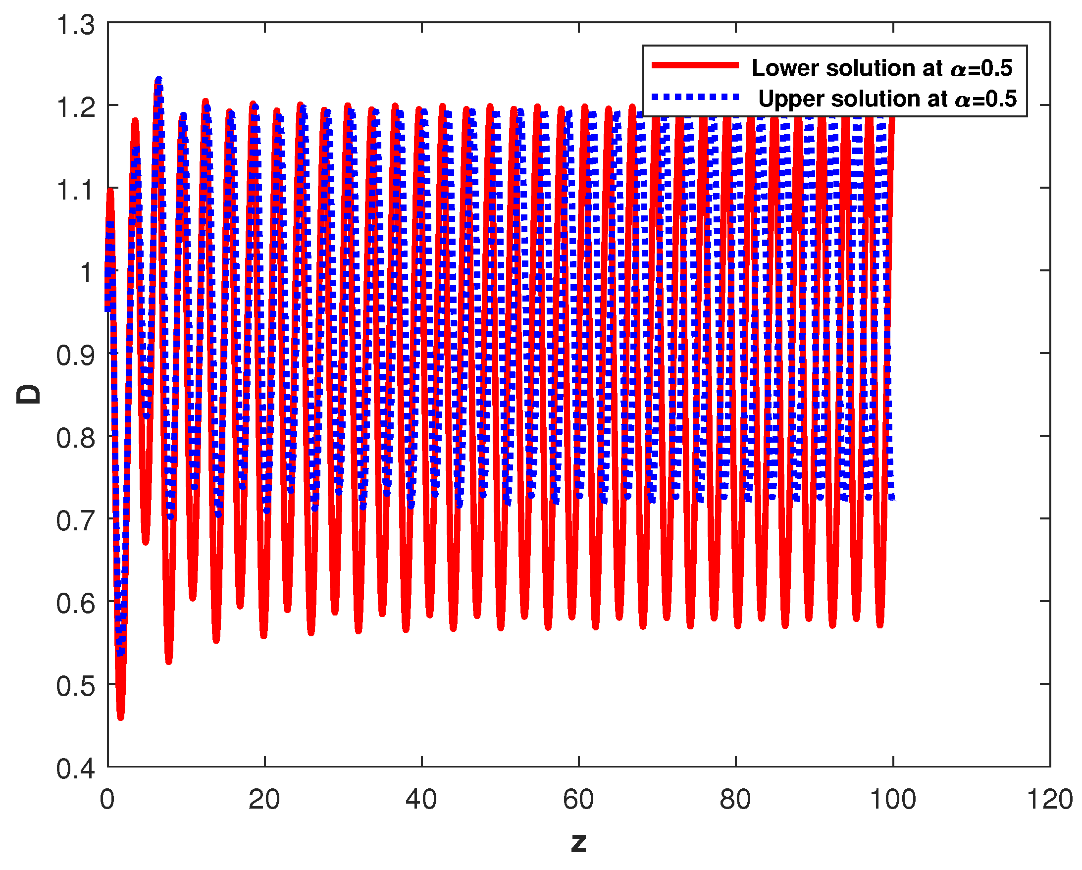
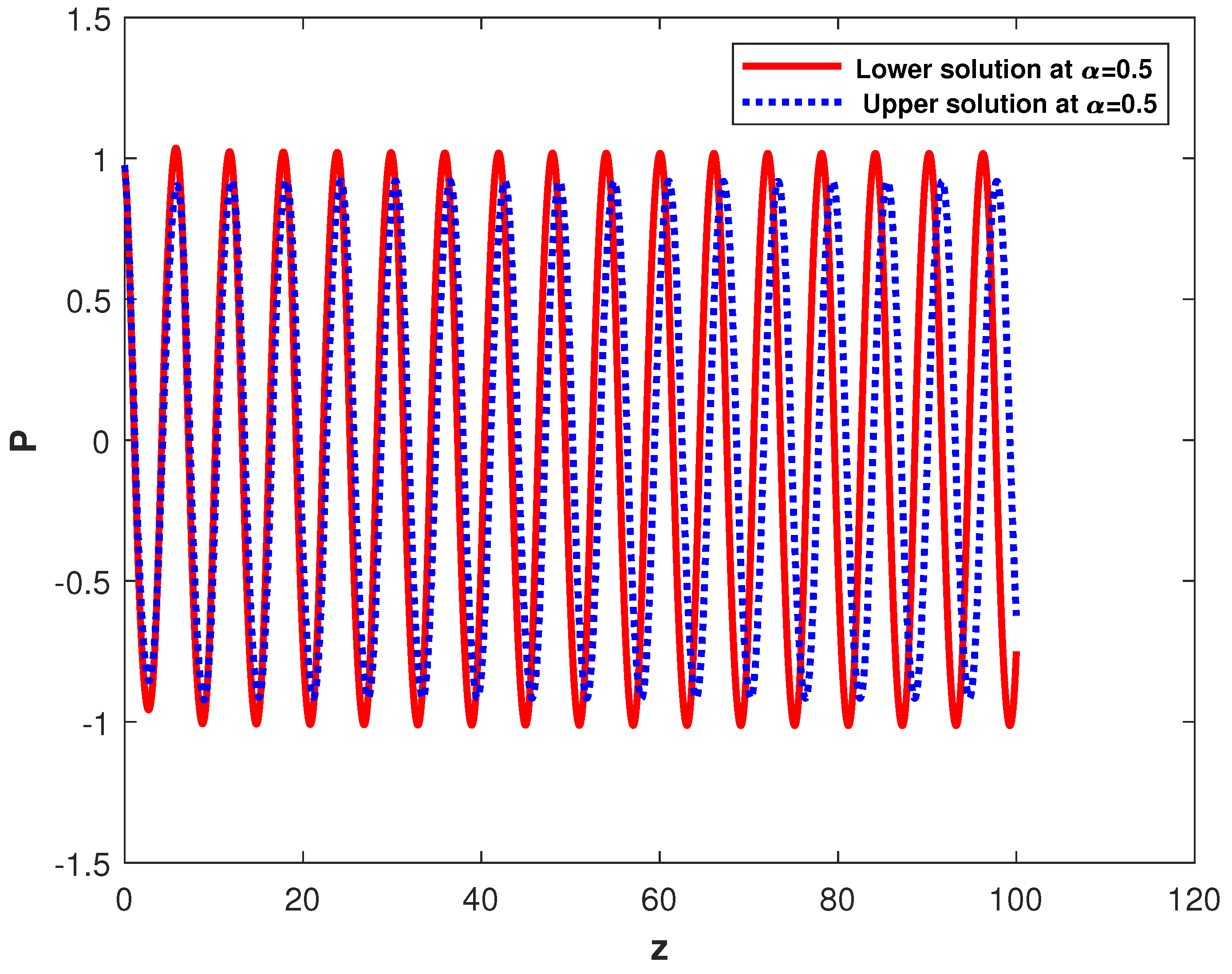
The graphical representation of the investment rate $\mathbb{I}$ in Figure 1, the investment cost $\mathbb{D}$ in Figure 2 and the price index $\mathbb{P}$ in Figure 3 were examined with the fractional order $\vartheta =0.9$ of system (4). This model incorporated the uncertain parameters and initial conditions represented through the triangular FNs, with the $\alpha$-cut interval evaluated at $\alpha =0.5$. In the graphical representation, the solid line denotes the lower end. In contrast, the dotted line signifies the upper end of the $\alpha$-cut, effectively illustrating a spectrum of potential trajectories under conditions of moderate uncertainty. The $\alpha$-cut interval for the investment rate $\mathbb{I}$ (in Figure 1) shows how vital uncertainty is to the trajectory of capital growth. The lower end (solid curve) indicates a gradual and stable increase in the investment rate, signifying a conservative scenario where savings and initial demand are limited. Similarly, the upper end (dotted curve) shows a more optimistic trajectory with higher growth and potential fluctuations, implying that favorable conditions lead to more rapid adjustments in investment. The gap between these bounds indicates the sensitivity of investment rates to initial economic circumstances. These limits suggest that slight changes in economic elements could significantly influence investment growth patterns. In the context of the investment demand denoted as $\mathbb{D}$ (in Figure 2), the $\alpha$-cut bounds show how the uncertainty impacts the expected expense. The lower end demonstrates a relatively consistent cost trajectory over a temporal spectrum, indicative of conservative market assumptions where costs remain controlled. Similarly, the upper bound indicates the higher potential costs associated with increased demand. The gap between these bounds reveals the impact of economic uncertainty on investment expenses with potential risk, which is associated with increased costs when demand or production factors fluctuate. For the price index $\mathbb{P}$ (in Figure 3), the $\alpha$-cut interval serves as a crucial analytical tool to discern inflationary or deflationary dynamics within the marketplace. The lower end indicates a state of price stability, which reflects a condition in which prices adjust gradually without significant inflation. In contrast, the upper end suggests the trend towards inflationary tendencies, where price levels increase in response to a stranger’s demand. This disparity between the bounds shows the potential instability in price level under FICs, signifying that the price index remains susceptible to inflationary pressures, particularly during periods of high demand or when demand elasticity is subject to fluctuations.

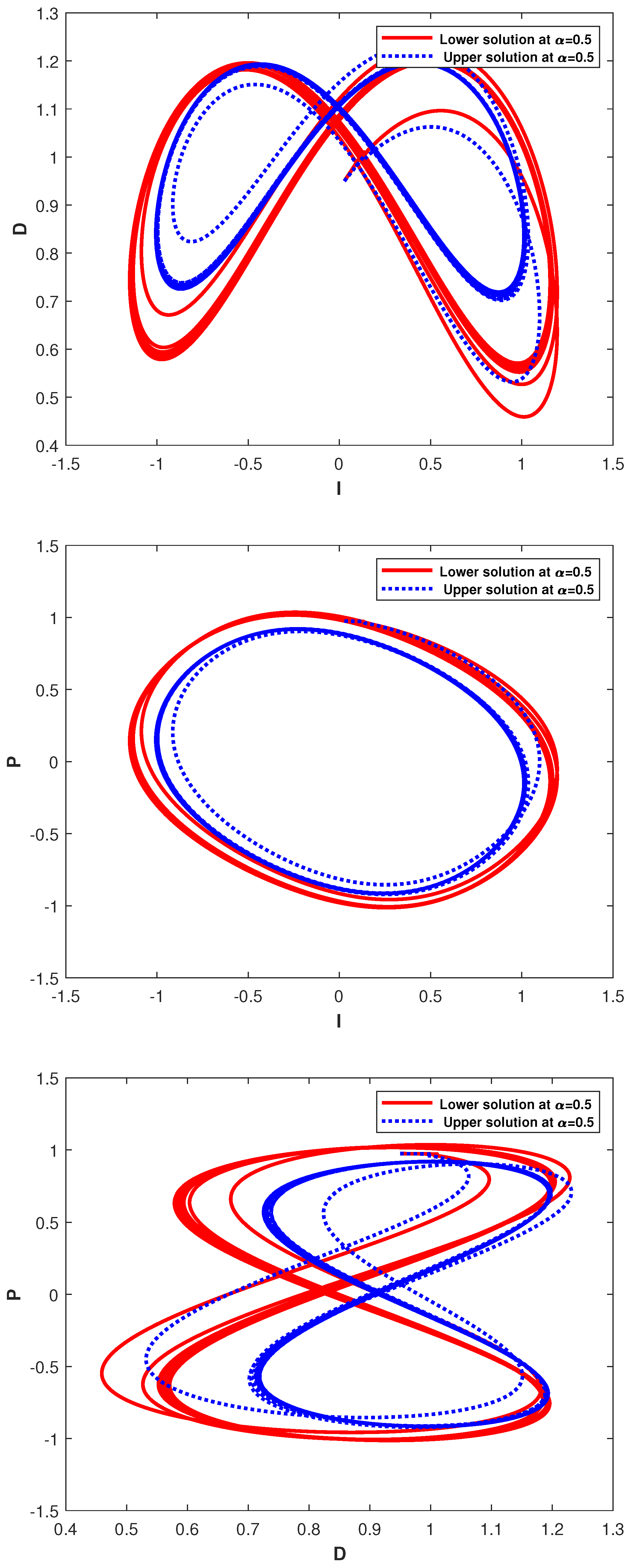
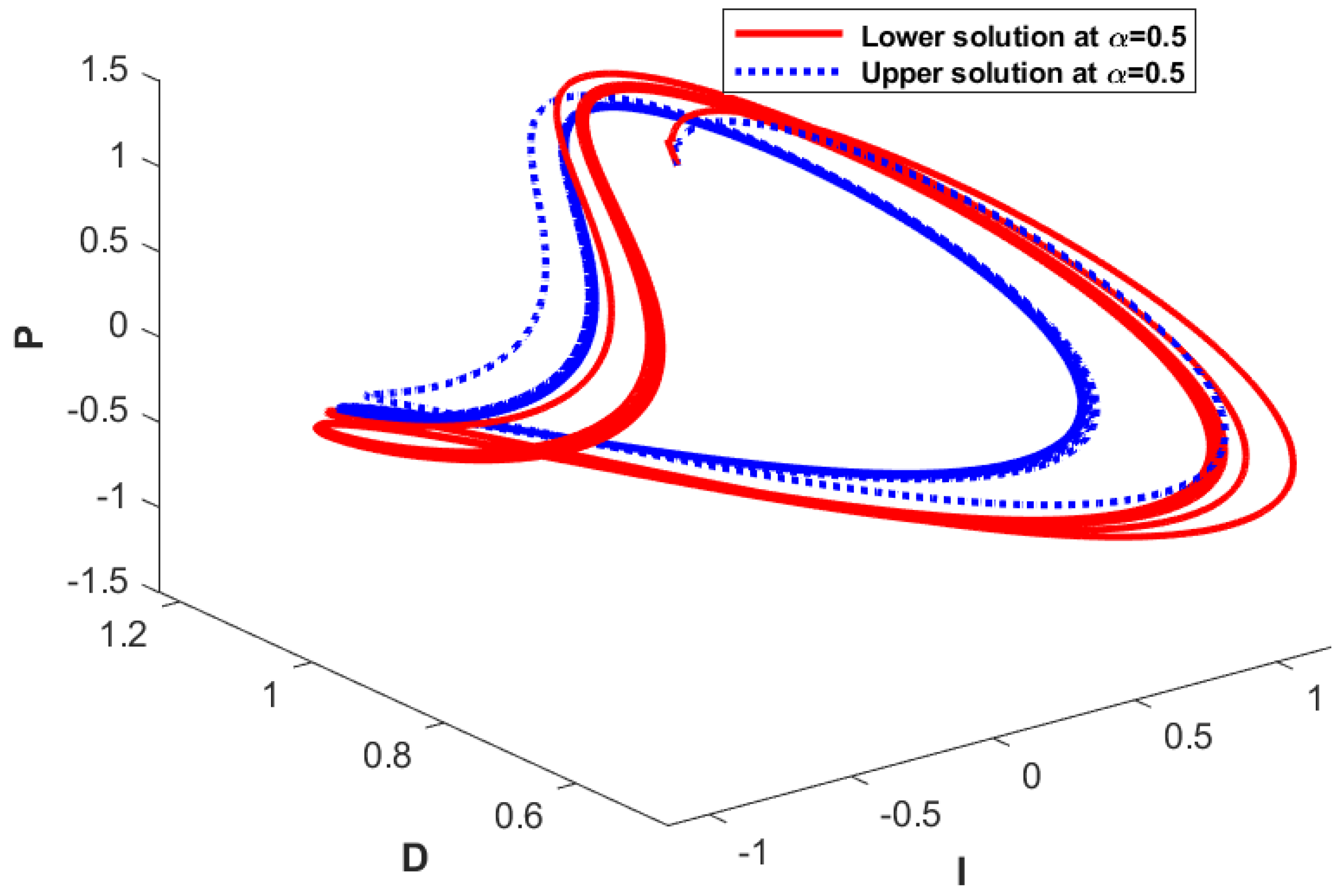
These graphical visualizations depict the pairwise and three-dimensional relationships among the investment rate $\mathbb{I}$, the investment cost $\mathbb{D}$, and the price index $\mathbb{P}$, as shown in Figure 4 and Figure 5, respectively, in the context of fuzziness using a fractional order of $\vartheta =0.9$. Each graphical representation includes a solid line that indicates the lower end and a dotted line that denotes the upper end of the $\alpha$-cut at $\alpha =0.5$. The graph of $\mathbb{I}$ and $\mathbb{D}$ indicates how changes in $\mathbb{I}$ interact with $\mathbb{D}$. The gap between the lower and upper bounds indicates the sensitivity of the FICs. This gap suggests a variety of potential economic outcomes under uncertain conditions with achievable investment levels that vary with the associated costs. The impact of the investment rate on the price index is investigated in the plot of $\mathbb{I}$ and $\mathbb{P}$. The upper and lower bounds represent the unpredictable consequences of investment on either deflationary or inflationary tendencies, depending on the economic assumptions. A broader gap between bounds indicates greater variability in the price response to investment levels, which provides information on the potential inflationary pressures associated with higher investments. The plot of $\mathbb{D}$ and $\mathbb{P}$ captures possible market reactions to variable costs by analyzing the relationship between price index changes and investment cost variations. The model sensitivity to changes in investment expenses is demonstrated by the range between solid and dotted lines, which shows that unknown costs can result in either stable pricing or inflationary price behavior depending on economic assumptions. These graphs visually capture the complex interdependence among $\mathbb{I}$, $\mathbb{D}$, and $\mathbb{P}$. These graphs also indicate how the uncertain parameters and initial conditions influence each variable differently. The $\alpha$-cut representations of the parameters and initial conditions enable a broader understanding of the model behavior and its characteristics, thus revealing possible dynamics under economic conditions. This uncertain analysis improves the predictive flexibility of the model by providing decision-makers with information on how shifting prices, costs, and investments may interact within a fractional differential framework.

5. Conclusions

This article introduced and investigated the granular fuzzy fractional financial model using the $gr$-CFD. The potential solution was determined using two approaches: an analytical scheme by applying the FLT technique and the introduced numerical technique using FIEs. Furthermore, the E&U of the proposed solution were determined using the Banach contraction principle. To analyze the nonlinearity of the proposed model, the introduced numerical scheme was employed to illustrate the uncertain behavior graphically. In the future, we will extend the proposed technique to analyze the behavior and function projection synchronization of fuzzy fractional financial risk systems to gain deeper insights into complex financial dynamics. The developed model improves the financial market process by improving risk prediction through gr-CFD, allowing more precise uncertainty assessments. In addition, it facilitates adaptive decision-making in unpredictable markets by capturing nonlinear financial dynamics under the fuzzy framework. This model also offers a computational tool for investors to analyze complex financial scenarios before implementing the policy or making investment choices. Future research will be conducted on the extension of the proposed technique to analyze behavioral synchronization in financial risk systems and to strengthen the connection between theoretical insights and real-world financial applications.

References

1. Dubois, D.; Prade, H. Towards fuzzy differential calculus part 3: Differentiation. Fuzzy Sets Syst. 1982, 8, 225–233. [Google Scholar] [CrossRef]
2. Akram, M.; Muhammad, G.; Allahviranloo, T.; Pedrycz, W. Solution of initial-value problem for linear third-order fuzzy differential equations. Comput. Appl. Math. 2022, 41, 398. [Google Scholar] [CrossRef]
3. Muhammad, G.; Akram, M. Fuzzy fractional epidemiological model for Middle East respiratory syndrome coronavirus on complex heterogeneous network using Caputo derivative. Inf. Sci. 2024, 659, 120046. [Google Scholar] [CrossRef]
4. Ahmad, S.; Ullah, A.; Ullah, A.; Hoa, N.V. Fuzzy natural transform method for solving fuzzy differential equations. Soft Comput. 2023, 27, 8611–8625. [Google Scholar] [CrossRef]
5. Akram, M.; Muhammad, G.; Allahviranloo, T. Explicit analytical solutions of an incommensurate system of fractional differential equations in a fuzzy environment. Inf. Sci. 2023, 645, 119372. [Google Scholar] [CrossRef]
6. Akram, M.; Muhammad, G.; Allahviranloo, T.; Pedrycz, W. Incommensurate non-homogeneous system of fuzzy linear fractional differential equations using the fuzzy bunch of real functions. Fuzzy Sets Syst. 2023, 473, 108725. [Google Scholar] [CrossRef]
7. Allahviranloo, T.; Ahmadi, M.B. Fuzzy Laplace transforms. Soft Comput. 2010, 14, 235–243. [Google Scholar] [CrossRef]
8. Effati, S.; Pakdaman, M. Artificial neural network approach for solving fuzzy differential equations. Inf. Sci. 2010, 180, 1434–1457. [Google Scholar] [CrossRef]
9. Muhammad, G.; Akram, M. Fuzzy fractional generalized Bagley-Torvik equation with fuzzy Caputo gH-differentiability. Eng. Appl. Artif. Intell. 2024, 133, 108265. [Google Scholar] [CrossRef]
10. Mazandarani, M.; Pan, J. The challenges of modeling using fuzzy standard interval arithmetic: A case study in electrical engineering. Inf. Sci. 2024, 653, 119774. [Google Scholar] [CrossRef]
11. Mazandarani, M.; Pariz, N.; Kamyad, A.V. Granular differentiability of fuzzy-number-valued functions. IEEE Trans. Fuzzy Syst. 2017, 26, 310–323. [Google Scholar] [CrossRef]
12. Chalco-Cano, Y.; Roman-Flores, H. On new solutions of fuzzy differential equations. Chaos Solitons Fractals 2008, 38, 112–119. [Google Scholar] [CrossRef]
13. Nabulsi, R.A.E.; Anukool, W. Qualitative financial modelling in fractal dimensions. Financ. Innov. 2025, 11, 42. [Google Scholar] [CrossRef]
14. Nikan, O.; Rashidinia, J.; Jafari, H. Numerically pricing American and European options using a time fractional Black–Scholes model in financial decision-making. Alex. Eng. J. 2025, 112, 235–245. [Google Scholar] [CrossRef]
15. Ahmad, I.; Jan, R.; Razak, N.N.A.; Khan, A.; Abdeljawad, T. Exploring Fractional-Order Models in Computational Finance via an Efficient Hybrid Approach. Eur. J. Pure Appl. Math. 2025, 18, 5793. [Google Scholar] [CrossRef]
16. Selvam, A.; Boulaaras, S.; Sabarinathan, S.; Radwan, T. Nonlinear fractional order financial system: Chaotic behavior and Ulam-Hyers stability. Fractals 2025, 33, 11–22. [Google Scholar] [CrossRef]
17. Bozkurt, M.A.; Köse, Y.; Çelik, S. Analyzing the dynamic behavior and market efficiency of green energy investments: A geometric and fractional brownian motion approach. Energy Sources Part B Econ. Plan. Policy 2025, 20, 2457438. [Google Scholar] [CrossRef]
18. Akgüller, Ö.; Balcı, M.A.; Batrancea, L.M.; Gaban, L. Fractional Transfer Entropy Networks: Short-and Long-Memory Perspectives on Global Stock Market Interactions. Fractal Fract. 2025, 9, 69. [Google Scholar] [CrossRef]
19. Bai, Y.; Kehoe, P.J.; Lopez, P.; Perri, F. A Neoclassical Model of the World Financial Cycle; Technical report; National Bureau of Economic Research: Cambridge, MA, USA, 2025. [Google Scholar]
20. Kumar, S.; ElKholy, M.; Liu, D.; Boulenger, A. Bridging the Gap: Efficient Cross-Lingual NER in Low-Resource Financial Domain. In Proceedings of the Joint Workshop of the 9th Financial Technology and Natural Language Processing, the 6th Financial Narrative Processing, and the 1st Workshop on Large Language Models for Finance and Legal, Abu Dhabi, United Arab Emirates, 19–20 January 2025; pp. 54–62. [Google Scholar]
21. Shone, R. Economic Dynamics: Phase Diagrams and Their Economic Application; Cambridge University Press: Cambridge, UK, 2002. [Google Scholar]
22. Chian, A.C.L.; Rempel, E.L.; Rogers, C. Complex economic dynamics: Chaotic saddle, crisis and intermittency. Chaos Solitons Fractals 2006, 29, 1194–1218. [Google Scholar] [CrossRef]
23. Wang, Z.; Huang, X.; Shi, G. Analysis of nonlinear dynamics and chaos in a fractional order financial system with time delay. Comput. Math. Appl. 2011, 62, 1531–1539. [Google Scholar] [CrossRef]
24. Elouahab, M.S.A.; Hamri, N.E.; Wang, J. Chaos control of a fractional-order financial system. Math. Probl. Eng. 2010, 18, 270646. [Google Scholar] [CrossRef]
25. Johansyah, M.D.; Sambas, A.; Qureshi, S.; Zheng, S.; Elhameed, T.M.A.; Vaidyanathan, S.; Sulaiman, I.M. Investigation of the hyperchaos and control in the fractional order financial system with profit margin. Partial. Differ. Equ. Appl. Math. 2024, 9, 100612. [Google Scholar] [CrossRef]
26. Olayiwola, M.O.; Alaje, A.I.; Yunus, A.O. A Caputo fractional order financial mathematical model analyzing the impact of an adaptive minimum interest rate and maximum investment demand. Results Control. Optim. 2024, 14, 100349. [Google Scholar] [CrossRef]
27. Li, S.; Khan, S.; Riaz, M.; AlQahtani, S.; Alamri, A. Numerical simulation of a fractional stochastic delay differential equations using spectral scheme: A comprehensive stability analysis. Sci. Rep. 2024, 14, 6930. [Google Scholar] [CrossRef]
28. Qayyum, M.; Ahmad, E.; Saeed, S.T.; Akgül, A.; Din, S.M.E. New solutions of fractional 4d chaotic financial model with optimal control via he-laplace algorithm. Ain Shams Eng. J. 2024, 15, 102503. [Google Scholar] [CrossRef]
29. Pakhira, R.; Mondal, B.; Ghosh, U.; Sarkar, S. An EOQ model with fractional order rate of change of inventory level and time-varying holding cost. Soft Comput. 2024, 28, 3859–3877. [Google Scholar] [CrossRef]
30. Liu, X.; Ye, G.; Liu, W.; Shi, F. Fuzzy discrete fractional granular calculus and its application to fractional cobweb models. Appl. Math. Comput. 2025, 489, 129176. [Google Scholar] [CrossRef]
31. Xu, X.; Wang, L.; Du, Z.; Kao, Y. H sampled-data control for uncertain fuzzy systems under Markovian jump and FBm. Appl. Math. Comput. 2023, 451, 128014. [Google Scholar] [CrossRef]
32. Xu, K.; Wang, H.; Liu, P. Adaptive fuzzy finite-time tracking control of nonlinear systems with unmodeled dynamics. Appl. Math. Comput. 2023, 450, 127992. [Google Scholar] [CrossRef]
33. Ali, M.; Narayanan, G.; Shekher, V.; Alsulami, H.; Saeed, T. Dynamic stability analysis of stochastic fractional-order memristor fuzzy BAM neural networks with delay and leakage terms. Appl. Math. Comput. 2020, 369, 124896. [Google Scholar]
34. Song, S.; Park, J.; Zhang, B.; Song, X. Adaptive hybrid fuzzy output feedback control for fractional-order nonlinear systems with time-varying delays and input saturation. Appl. Math. Comput. 2020, 364, 124662. [Google Scholar] [CrossRef]
35. Xu, Z.; Sun, K.; Wang, H. Dynamics and function projection synchronization for the fractional-order financial risk system. Chaos Solitons Fractals 2024, 188, 115599. [Google Scholar] [CrossRef]
36. Mesgarani, H.; Aghdam, Y.E.; Beiranvand, A.; Gómez-Aguilar, J. A novel approach to fuzzy based efficiency assessment of a financial system. Comput. Econ. 2024, 63, 1609–1626. [Google Scholar] [CrossRef]
37. Qayyum, M.; Ahmad, E.; Sohail, M.; Sarhan, N.; Awwad, E.M.; Iqbal, A. Design and implementation of fuzzy-fractional Wu–Zhang system using He–Mohand algorithm. Fractals 2024, 32, 2440032. [Google Scholar] [CrossRef]
38. Johansyah, M.D.; Hamidzadeh, S.M.; Benkouider, K.; Vaıdyanathan, S.; Sambas, A.; Mohamed, M.A.; Aziz, A.A. A Novel Hyperchaotic Financial System with Sinusoidal Hyperbolic Nonlinearity: From Theoretical Analysis to Adaptive Neural Fuzzy Controller Method. Chaos Theory Appl. 2024, 6, 26–40. [Google Scholar] [CrossRef]
39. Qayyum, M.; Ahmad, E.; Akgül, A.; Din, S.M.E. Fuzzy-fractional modeling of Korteweg-de Vries equations in Gaussian-Caputo sense: New solutions via extended He-Mahgoub algorithm. Ain Shams Eng. J. 2024, 15, 102623. [Google Scholar] [CrossRef]
40. Qayyum, M.; Ahmad, E.; Tahir, A.; Acharya, S. Modeling and analysis of the fuzzy-fractional chaotic financial system using the extended He–Mohand algorithm in a fuzzy-Caputo sense. Int. J. Intell. Syst. 2023, 2023, 3028824. [Google Scholar] [CrossRef]
41. Aderyani, S.R.; Saadati, R.; Allahviranloo, T.; Abbasbandy, S.; Catak, M. Fuzzy approximation of a fractional Lorenz system and a fractional financial crisis. Iran. J. Fuzzy Syst. 2023, 20, 27–36. [Google Scholar]
42. Bian, L.; Li, Z. Fuzzy simulation of European option pricing using sub-fractional Brownian motion. Chaos Solitons Fractals 2021, 153, 111442. [Google Scholar] [CrossRef]
43. Rehman, Z.U.; Boulaaras, S.; Jan, R.; Ahmad, I.; Bahramand, S. Computational analysis of financial system through non-integer derivative. J. Comput. Sci. 2024, 75, 102204. [Google Scholar] [CrossRef]
44. Alsenafi, A.; Alazemi, F.; Najafi, A. Geometric Asian power option pricing with transaction cost under the geometric fractional Brownian motion with w sources of risk in fuzzy environment. J. Comput. Appl. Math. 2025, 453, 116165. [Google Scholar] [CrossRef]
45. Nand, A. Next-generation inventory optimization: Advanced inventory management harnessing demand variability integrating fuzzy logic and granular differentiability. RAIRO Oper. Res. 2025, 59, 335–353. [Google Scholar] [CrossRef]
46. Brar, J.; Braun, J.; Hare, W.; Wang, D. A simulation analysis of returns-risk portfolio optimization models. Commun. Stat. Simul. Comput. 2025, 20, 1–28. [Google Scholar] [CrossRef]
47. Xiong, T.; Liu, Z.; Zhang, M. Evaluating the efficacy of fuzzy Bayesian networks for financial risk assessment. Demonstr. Math. 2025, 58, 20240032. [Google Scholar] [CrossRef]
48. Babakordi, F.; Allahviranloo, T.; Shahriari, M.R.; Catak, M. Fuzzy Laplace transform method for a fractional fuzzy economic model based on market equilibrium. Inf. Sci. 2024, 665, 120308. [Google Scholar] [CrossRef]
49. Sukono; Sambas, A.; He, S.; Liu, H.; Vaidyanathan, S.; Hidayat, Y.; Saputra, J. Dynamical analysis and adaptive fuzzy control for the fractional-order financial risk chaotic system. Adv. Differ. Equ. 2020, 2020, 674. [Google Scholar] [CrossRef]
50. Hashemi, H.; Ezzati, R.; Mikaeilvand, N.; Nazari, M. Study on fuzzy fractional European option pricing model with Mittag-Leffler kernel. J. Intell. Fuzzy Syst. 2023, 45, 8567–8582. [Google Scholar] [CrossRef]
51. Rahaman, M.; Mondal, S.P.; Chatterjee, B.; Alam, S.; Shaikh, A.A. Generalization of classical fuzzy economic order quantity model based on memory dependency via fuzzy fractional differential equation approach. J. Uncertain Syst. 2022, 15, 2250003. [Google Scholar] [CrossRef]
52. Bede, B.; Stefanini, L. Generalized differentiability of fuzzy-valued functions. Fuzzy Sets Syst. 2013, 230, 119–141. [Google Scholar] [CrossRef]
53. Piegat, A.; Landowski, M. Horizontal membership function and examples of its applications. Int. J. Fuzzy Syst. 2015, 17, 22–30. [Google Scholar] [CrossRef]
54. Son, N.T.K.; Long, H.V.; Dong, N.P. Fuzzy delay differential equations under granular differentiability with applications. Comput. Appl. Math. 2019, 38, 107. [Google Scholar] [CrossRef]
55. Dong, N.P.; Long, H.V.; Khastan, A. Optimal control of a fractional order model for granular SEIR epidemic with uncertainty. Commun. Nonlinear Sci. Numer. Simul. 2020, 88, 105312. [Google Scholar] [CrossRef] [PubMed]
56. Najariyan, M.; Zhao, Y. Fuzzy fractional quadratic regulator problem under granular fuzzy fractional derivatives. IEEE Trans. Fuzzy Syst. 2017, 26, 2273–2288. [Google Scholar] [CrossRef]
57. Long, H.V.; Dong, N.P. An extension of Krasnoselskii’s fixed point theorem and its application to nonlocal problems for implicit fractional differential systems with uncertainty. J. Fixed Point Theory Appl. 2018, 20, 37. [Google Scholar] [CrossRef]
58. Long, H.V.; Son, N.T.K.; Tam, H.T.T.; Yao, J.C. Ulam stability for fractional partial integro-differential equation with uncertainty. Acta Math. Vietnam. 2017, 42, 675–700. [Google Scholar] [CrossRef]
Figure 1. The plot of the investment rate I with the fractional order ϑ = 0.9 , where the solid curve represents the lower end, and the dotted curve represents the upper end of the α -cut of the solution by taking α = 0.5 (from left to right).
Mathematics 13 01240 g001
Figure 2. The plot of the investment demand D with the fractional order ϑ = 0.9 , where the solid curve represents the lower end, and the dotted curve represents the upper end of the α -cut of the solution by taking α = 0.5 (from left to right).
Mathematics 13 01240 g002
Figure 3. The plot of the price index P with the fractional order ϑ = 0.9 , where the solid curve represents the lower end, and the dotted curve represents the upper end of the α -cut of the solution by taking α = 0.5 (from left to right).
Mathematics 13 01240 g003
Figure 4. These plots show the relationship between I and D , I and P , and D and P with the fractional order ϑ = 0.9 , where the solid curve represents the lower end, and the dotted curve represent the upper end of the α -cut of the solution by taking α = 0.5 (from left to right).
Mathematics 13 01240 g004
Figure 5. Three-dimensional visualization of I , D , and P with the fractional order ϑ = 0.9 , where the solid curve represents the lower end, and the dotted curve represent the upper end of the α -cut of the solution by taking α = 0.5 (from left to right).
Mathematics 13 01240 g005