A Framework for Breast Cancer Classification with Deep Features and Modified Grey Wolf Optimization

Abstract

Breast cancer is the most common disease in women, with 287,800 new cases and 43,200 deaths in 2022 across United States. Early mammographic picture analysis and processing reduce mortality and enable efficient treatment. Several deep-learning-based mammography classification methods have been developed. Due to low-contrast images and irrelevant information in publicly available breast cancer datasets, existing models generally perform poorly. Pre-trained convolutional neural network models trained on generic datasets tend to extract irrelevant features when applied to domain-specific classification tasks, highlighting the need for a feature selection mechanism to transform high-dimensional data into a more discriminative feature space. This work introduces an innovative and effective multi-step pathway to overcome these restrictions. In preprocessing, mammographic pictures are haze-reduced using adaptive transformation, normalized using a cropping algorithm, and balanced using rotation, flipping, and noise addition. A 32-layer convolutional neural model inspired by YOLO, U-Net, and ResNet is intended to extract highly discriminative features for breast cancer classification. A modified Grey Wolf Optimization algorithm with three significant adjustments improves feature selection and redundancy removal over the previous approach. The robustness and efficacy of the proposed model in the classification of breast cancer were validated by its consistently high performance across multiple benchmark mammogram datasets. The model’s constant and better performance proves its robust generalization, giving it a powerful solution for binary and multiclass breast cancer classification.

1. Introduction

Breast cancer is the cruelest disease for women [1]. First, breast tissues are attacked, followed by others. This makes breast cancer one of the most ruthless female cancers. The WHO found that 8% are diagnosed and 6% die [2]. Approximately 8% of women develop this cancer. Around 43,000 died from this cancer in 2022. Malignant or benign tumors are present in this form of cancer. The first variety is particularly cruel, as it infiltrates the tissues in its vicinity, while the second type does not. Consequently, malignant lesions are particularly hazardous to women [3]. Numerous imaging techniques can be employed to diagnose this tumor. In general, biopsy is a practical method due to its precision. Nevertheless, numerous studies recommend that women refrain from undergoing multiple biopsies for the purposes of diagnosis and treatment [4]. Breast cancer is diagnosed more promptly using ultrasound (US) breast image samples in computer-aided diagnosis (CAD). Liquid-filled cysts can be distinguished from solid lesions using breast ultrasounds. Breast ultrasound images are non-invasive, radiation-free, and can provide clinicians with guidance during biopsy operations.

Table 1. List of abbreviations.

Abbreviation	Definition	Abbreviation	Definition
AI	Artificial Intelligence	CAD	Computer-Aided Diagnosis
CNN	Convolutional Neural Network	DDSM	Digital Database for Screening Mammography
DL	Deep Learning	FN	False Negative
FP	False Positive	HRAT	Haze-Removed Adaptive Technique
INbreast	Full-Field Digital Mammogram Dataset	MIAS	Mammographic Image Analysis Society
ML	Machine Learning	mGWO	Modified Grey Wolf Optimization
NN	Neural Network	PSO	Particle Swarm Optimization
ROI	Region of Interest	TN	True Negative
TP	True Positive	YOLO	You Only Look Once

provides a list of abbreviations used in this work.

The vast number of mammograms radiologists must analyze daily and the difficulty of finding troublesome areas makes the procedure complex, expensive, and risky. Thus, innovative and sophisticated methods for breast cancer detection are needed. Deep learning (DL) convolutional neural networks (CNNs) have improved mammography analysis. Recent research shows the CNN’s promise to tackle this field’s difficulties. Several articles have examined deep learning in mammography analysis. The CNN requires a lot of training data, which can limit them. Automatically detecting and highlighting tumors, organs, arteries, and cells in medical images requires image segmentation. U-Net, a CNN-based encoder–decoder network, is the industry standard for medical image segmentation. U-Net and its descendants, such as Connected-UNet [5] and AU-Net [6], can recognize breast lumps with limited labeled training data. However, image regions of interest are still challenging to identify.

Deep learning algorithms for breast cancer detection and classification have improved, but key obstacles remain. Deep architectures like ResNet, YOLO, and Capsule Networks [7] demand a lot of processing power, limiting real-time clinical use. Small, imbalanced datasets such as MIAS [8], DDSM [9], and INbreast [10] do not necessarily translate well to different real-world circumstances, resulting in overfitting and dataset dependency. Lesion detection methods still produce false positives and negatives, resulting in unnecessary medical procedures or missing diagnoses. Many models use transfer learning from pre-trained networks like ResNet50 and VGG16, built for natural images rather than mammograms, causing domain adaption difficulties. Traditional CNNs struggle to capture fine-grained lesion characteristics, especially in discriminating malignant from benign instances with high specificity.

In cancer recurrence and disease occurrence management, high-throughput technologies have advanced recently. The above improvements have produced different high-dimensional data. Every piece of medical data has a unique worth. Data interpretation becomes more complicated as dimensionality increases. Dimensionality reduction methods are needed to minimize the dimensions of high-dimensional data. Categorization, display, transmission, and storage are used in data reduction to manage multidimensional data. According to studies [11], poor data quality might include noise, abnormalities, data paucity or duplication, and biased or unrepresentative data. Dimensionality reduction may also remove unused features. This approach may reduce the number of interconnected features.

Discriminatory qualities are found using well-known feature selection methods [12,13]. Classification algorithms need potent features to create intelligent models. FS enhances classification accuracy and conserves computational resources in ML algorithm design and implementation [14,15]. An inappropriate or duplicated feature space may harm classifier performance. Feature selection algorithms select the most significant qualities from the initial set to increase classifier accuracy by reducing redundant features. Researchers have created and deployed various bio-inspired computer solutions to minimize feature space. Numerous studies show that classification systems’ accuracy depends on thorough feature selection [16,17].

In the context of medical imaging and analysis, DL techniques encounter challenges, particularly in the classification of breast tumors. The initial concern is the restricted availability of mammograms, as deep learning necessitates additional inputs to facilitate practical training and prospective solutions [18,19]. The subsequent phase is featuring engineering, which involves the development of redundant deep features that affect the efficacy and computation of classification [20,21]. The paper proposes a CAD architecture that integrates deep features with enhanced and distinctive mammography. The main contributions are as follows:

• Utilization of three distinct mammographic databases to evaluate the suggested approach thoroughly.
• The Haze-Removed Adaptive Technique (HRAT) improves contrast adjustment and image clarity.
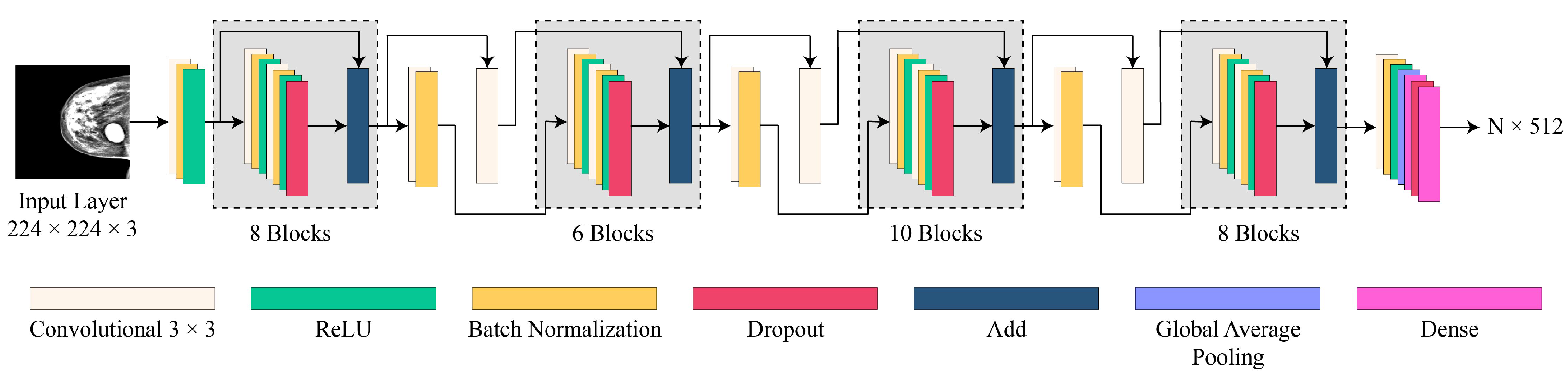
• Designing a 32-layer CNN model for breast cancer mammographic data based on YOLO, U-Net, and ResNet.
• The modified Grey Wolf Optimization (mGWO) approach to extract highly discriminative features, minimize redundancy, and improve classification.

The organization of the paper is as follows: Section 2 summarizes relevant prior research. Section 3 details the experimental design, dataset, methodology, and strategies used in the study. Section 4 analyzes the findings and comments, including performance measurements, experiments, parameter selection, and comparisons to existing approaches. We conclude with future directions in Section 5.

2. Literature Review

As mentioned, breast cancer is the most common cancer. About 1.7 million women were reported worldwide in 2012. Due to age, family, and medical history, around 2 million new breast cancer cases are expected each year, which is worrying. Strikingly, 60,000 women were threatened by cancer diseases in 2018, and 15% of breast cancer patients died [22,23]. In breast tumor identification and classification, CAD frameworks, especially deep learning (DL) techniques, improve tool performance. Mammogram samples always make erroneous forecasts due to tumor dangers and obstacles [24,25,26]. To find promising breast cancer diagnosis solutions, the CAD framework and proper DL techniques are more important.

A five-layer CNN model (four convolutional layers and one fully connected layer) [27] classified breast cancer using mammograms and ultrasound images with data augmentation for generalization. The method in [28] involves preprocessing and CNN-based classification. Enhancement, ROI extraction, noise removal, enlargement, and scaling are preprocessing steps. A CNN model is created from scratch for mammography feature learning and lesion classification. In [29], ResNet-50 CNN with ImageNet transfer learning was used to diagnose breast cancer. INbreast photos are classified as benign or cancerous by the model. Comparing experimental findings to other models on the same dataset shows 93.00% accuracy.

This study used Faster R-CNN for mass detection in the massive OMI-DB mammography dataset [30]. Training the model with Hologic scanning pictures achieves high accurate favorable rates. The INbreast dataset and GE scanner pictures apply transfer learning to detect masses. The study in [31] proposed an integrated CAD system for classification using YOLO for breast lesion detection and CNN-based classifiers (CNN, ResNet-50, InceptionResNet-V2). The system performs well in detecting and classifying DDSM and INbreast datasets with 5-fold cross-validation. YOLO architectures (YOLOv3, YOLOv5, YOLOv5-Transformer) with transfer learning on CBIS-DDSM, INbreast, and a proprietary dataset were used to create an automated breast cancer detection model [32]. Eigen-CAM aids interpretation. The performance was better with YOLOv5. A stacked ensemble of ResNet models (ResNet50V2, ResNet101V2, ResNet152V2) with an XGBoost classifier was used to classify breast mass, BI-RADS, and shape [33]. CBIS-DDSM, INbreast, and a private dataset show high accuracy for the model. Using transfer learning on NASNet Mobile and fine-tuning VGG16/VGG19, ref. [34] categorized mammography pictures using the BI-RADS scale. Multi-category categorization using deep learning was evaluated on the INbreast dataset with good accuracy and AUC.

Digital mammograms were used to develop the OMLTS-DLCN breast cancer diagnosis model [35]. It used adaptive fuzzy filtering to remove noise, optimum Kapur’s multi-level thresholding for segmentation, and BPNN-based CapsNet-based feature extractor for classification. ROI is divided into small areas for focused abnormality detection [36], reducing computer complexity. Noise-tolerant textural descriptors improve feature extraction and preserve regional patterns. On the DDSM dataset, SVM with grid search optimization classifies mammograms accurately. The study in [37] boosts mammography contrast by haze-reducing and augmenting. EfficientNet-B4 fuses original and upgraded images to extract features using a mid-value technique. On INbreast and CBIS-DDSM, chaotic-crow search optimizes features and ensures that ML classifiers are accurate. Morphological techniques for breast region extraction, bicubic interpolation for super-resolution, and data augmentation improve mammography diagnosis [38]. A unique 11-feature vector is produced for classification using the multiclass MIAS dataset, enhancing diagnostic accuracy. Two-view mammograms are used to classify benign and malignant breast tumors using a CNN-RNN model [39]. The modified ResNet extracts features from CC and MLO perspectives, whereas GRU merges spatial associations. The model classifies well on the DDSM dataset after training and testing. The summary of these studies is presented in

Table 2. Summary of studies included in the literature.

Method	Results (%)
A five-layer CNN model with data augmentation was used for automated breast cancer classification in mammograms and ultrasound images [27]	MIAS: 96.55 DDSM: 90.68 INbreast: 91.28
CNN-based classification with preprocessing for mammogram image enhancement and lesion detection [28]	INbreast: 96.52 MIAS: 95.30
Transfer learning with ResNet-50 trained on ImageNet [29]	INbreast: 93.00
Faster R-CNN for detecting masses in FFDM mammograms [30]	Hologic: TPR 93.00 INbreast: 99.00
YOLO for lesion detection, CNN/InceptionResNet-V2 for classification [31]	DDSM: 99.17 INbreast: 97.27
YOLO-based breast cancer detection with transfer learning and Eigen-CAM for model explainability [32]	CBIS-DDSM: mAP 62.10
Stacked ensemble of ResNet models with XGBoost for breast mass classification and BI-RADS diagnosis [33]	DDSM: 95.13 INbreast: 99.20 Private dataset: 95.88
VGG16/VGG19 fine-tuned on mammogram datasets for lesion classification [34]	INbreast: 96.52
CapsNet with adaptive fuzzy filtering and Kapur’s thresholding [35]	Mini-MIAS: 98.50 DDSM: 97.55
ROI-based patch segmentation with noise-tolerant textural descriptors and SVM classification [36]	DDSM: 94.70
EfficientNet-B4 with contrast enhancement, feature fusion, and chaotic-crow search optimization for classification [37]	INbreast: 98.45 DDSM: 96.17
Breast region extraction, super-resolution enhancement, and feature-based classification for mammography [38]	MIAS: 97.14
Two-view CNN-RNN model with ResNet and GRU for breast mass classification [39]	DDSM: 94.70

.

Deep learning algorithms for breast cancer detection and classification have improved, but key obstacles remain. Deep architectures like ResNet, YOLO, and Capsule Networks demand a lot of processing power, limiting real-time clinical use [40]. Small, imbalanced datasets such as INbreast, DDSM, and MIAS do not necessarily translate well to different real-world circumstances, resulting in overfitting and dataset dependency. Lesion detection methods still produce false positives and negatives, resulting in unnecessary medical procedures or missing diagnoses. Many models use transfer learning from pre-trained networks like ResNet50 and VGG16, built for natural pictures rather than mammograms, causing domain adaption difficulties. Traditional CNNs struggle to capture fine-grained lesion characteristics, especially in discriminating malignant from benign instances with high specificity. Feature optimization is essential to fix these concerns. Automated feature selection, hybrid feature fusion, and metaheuristic optimization (e.g., evolutionary algorithms, Particle Swarm Optimization, Bayesian optimization) can enhance classification accuracy and reduce computational load. Multi-scale feature extraction employing graph-based representations and attention mechanisms may improve lesion characterization. Adaptive feature weighting may also increase model resilience across datasets. Feature extraction and selection procedures should be optimized to enhance classification effectiveness, false detections, and clinical application.

3. Materials and Methods

This section discusses the dataset, preprocessing techniques, and proposed farmwork to classify digital mammograms in detail for better understanding.

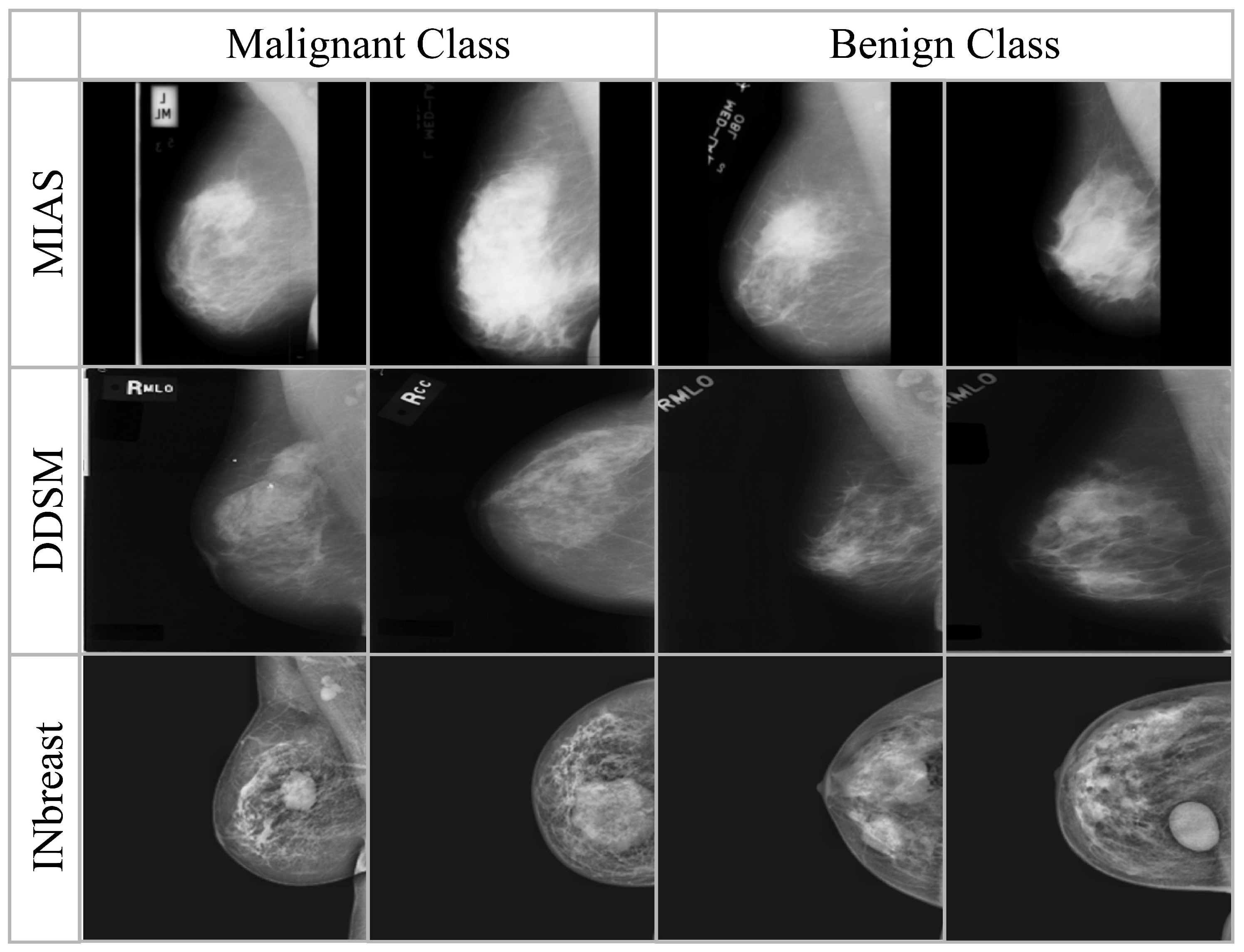
3.1. Mammogram Datasets

This research utilized mammogram images from three publicly available datasets: MIAS, DDSM, and INbreast. DDSM is a curated subgroup of regular DDSM (Digital Database for Screening Mammograms) and contains different breast imagery samples. The INbreast dataset blends several FFDMs (Full Field Digital Mammograms). The samples of the INbreast dataset provide more useful facts than the mammogram images of the DDSM database. The researchers also commonly use the MIAS dataset, which has 322 mammogram images of $1024\times 1024$ size. This dataset includes aberrant and normal photos. The two types of abnormal images are benign and malignant. This study utilized a total of 1572 original mammography images from three benchmark datasets: 300 photos from MIAS (39 malignant, 52 benign, 209 normal), 1194 images from DDSM (637 malignant, 557 benign), and 152 images from INbreast (70 malignant, 76 benign). The data were randomly and equitably divided into training and testing sets, maintaining class balance by stratified sampling. The utilization of these datasets shows that they are very famous in the breast cancer research community and considered standard for assessing models. Sample images from selected datasets for malignant and benign classes are shown in Figure 1, whereas the summary of each dataset is presented in

Table 3. Summary of selected datasets across malignant, benign, and normal class.

Dataset	Training Images			Testing Images			Total Images
	Mal	Ben	Nor	Mal	Ben	Nor	Mal	Ben	Nor
MIAS	19	26	104	20	26	105	39	52	209
DDMS	318	278	-	319	279	-	637	557	-
INbreast	35	38	-	35	38	-	70	76	-

.

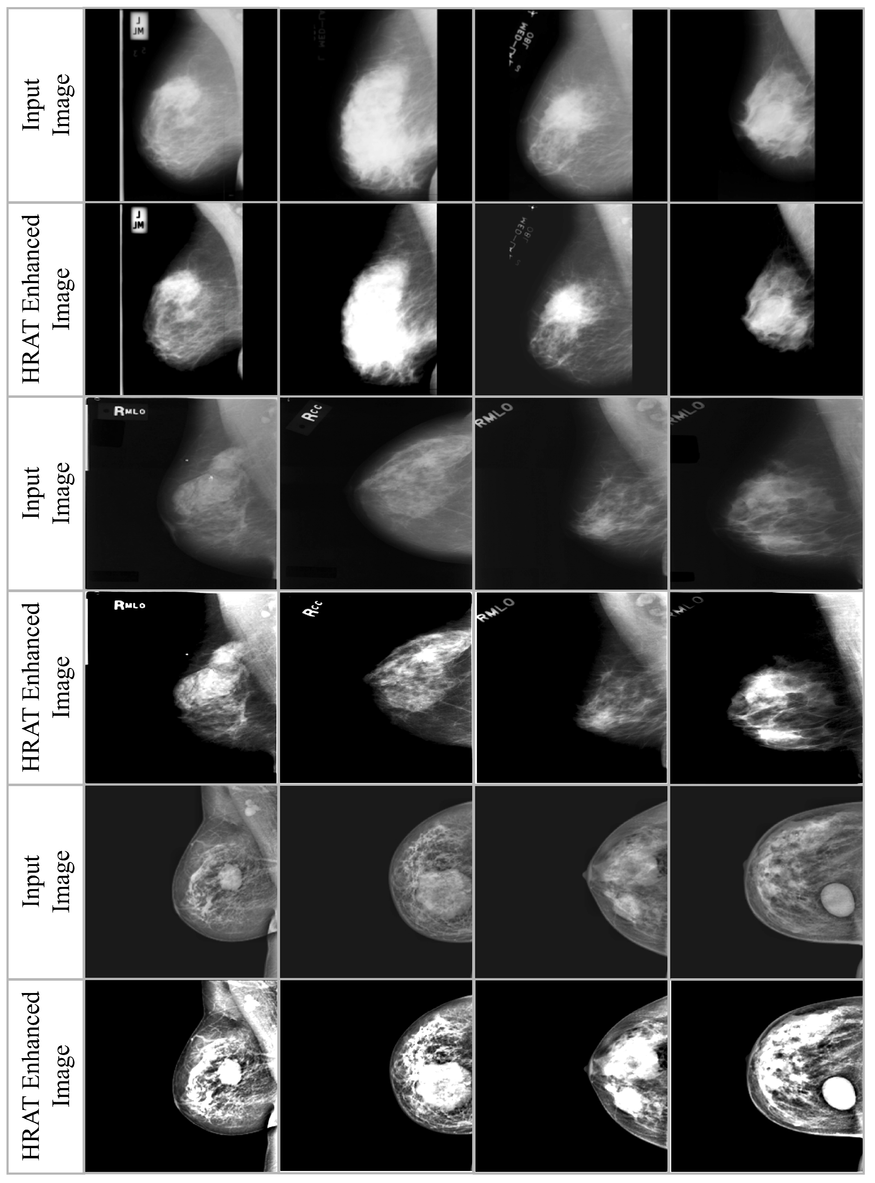
3.2. Haze-Removed Adaptive Technique (HRAT)

For the best breast tumor classification, contrast enhancement of digital mammograms is a very in-demand technique. The standard haze removal algorithm provides better-quality regenerated images with saturation and contrast adjustments. The haze removal algorithm made the lesions and micro-classifications visible in mammogram images. Thus, the Haze-Removed Adaptive Technique (HRAT) is developed to enhance contrast by combining adaptive global local transformation with the haze reduction algorithm. The original and contrast-enhanced mammogram images are shown in Figure 2.

The HRAT algorithm is designed for haze removal and adaptive transformation in mammogram images. Step 1 involves importing mammograms from both datasets. Step 2 uses dark channel-based haze reduction. The image’s dark channel, local minima for area IL (p) for all channels of the image pixels $(p,q)$ in the dataset, and minimum dark channel $D\left(a\right)$ value at intensity $(p,q)$ levels are calculated using a local window size for analysis as follows:

$$D(p,q)=d_{min}\left(min\left\{(p^{\prime },q^{\prime })\in I_L\left(p\right)\right\}s\left(I(p^{\prime },q^{\prime },i)\right)\right)$$

(1)

The intensity of a pixel in each channel and its local region determines its dark channel value. $D(p,q)$ is the dark channel value for the pixel $(p,q)$, $I(p^{\prime },q^{\prime },i)$ is the intensity in the channel I at pixel $\left(p{,}^{\prime }{q}^{\prime }\right)$, and $I_L\left(p\right)$ is the local region for pixel $(p,q)$. Consider a $3\times 3$ patch of a mammogram image with the following pixel intensity values in the RGB channels:

$$R=\left[\begin{array}{ccc}120& 100& 90\\ 80& 70& 110\\ 130& 95& 85\end{array}\right],G=\left[\begin{array}{ccc}115& 105& 95\\ 75& 65& 108\\ 125& 100& 88\end{array}\right],B=\left[\begin{array}{ccc}118& 102& 92\\ 78& 68& 107\\ 128& 98& 86\end{array}\right]$$

(2)

First, compute the minimum intensity at each pixel across the R, G, and B channels:

$$\begin{array}{c}\hfill \underset{RGB}{min}=\left[\begin{array}{ccc}min(120,115,118)& min(100,105,102)& min(90,95,92)\\ min(80,75,78)& min(70,65,68)& min(110,108,107)\\ min(130,125,128)& min(95,100,98)& min(85,88,86)\end{array}\right]\\ \hfill =\left[\begin{array}{ccc}115& 100& 90\\ 75& 65& 107\\ 125& 95& 85\end{array}\right]\end{array}$$

(3)

Now, apply Equation (1) by finding the minimum value within this $3\times 3$ patch:

$$D(p,q)=min(\underset{RGB}{min})=min\{115,100,90,75,65,107,125,95,85\}=\begin{array}{|c|}\hline 65\\ \hline\end{array}$$

(4)

Therefore, the dark channel value $D(p,q)$ at the center of this patch is 65, which will be used for haze estimation. Step 3 uses local and global adaptive transformation to improve image contrast. A contrast-enhanced pixel value is calculated using adaptive histogram equalization to enhance visibility as follows:

$$\mathrm{CEI}\left(I\right(p,q,i\left)\right)=\mathrm{ad}\_\mathrm{histeq}\left(I\right(p,q,i\left)\right)$$

(5)

Here, $\mathrm{CEI}\left(I\right(p,q,i\left)\right)$ is the contrast-enhanced pixel value for $(p,q)$ location in the channel I, and $\mathrm{ad}\_\mathrm{histeq}\left(I\right(p,q,i\left)\right)$ is the adaptive histogram equalization technique. Consider a small $3\times 3$ grayscale image patch:

$$I=\left[\begin{array}{ccc}52& 55& 61\\ 60& 59& 55\\ 58& 57& 54\end{array}\right]$$

(6)

For the center pixel (value = 59), the local histogram of the $3\times 3$ region is as follows:

$$\mathrm{Histogram}=\{52:1,54:1,55:2,57:1,58:1,59:1,60:1,61:1\}$$

(7)

The cumulative distribution function (CDF) is computed as follows:

$$\mathrm{CDF}\left(v\right)=\sum _{i\le v}{\displaystyle \frac{h\left(i\right)}{9}}$$

(8)

For pixel intensity 59,

$$\mathrm{CDF}\left(59\right)={\displaystyle \frac{1+1+2+1+1+1}{9}}={\displaystyle \frac{7}{9}}$$

(9)

Adaptive histogram equalization maps this to

$$CEI\left(59\right)=\mathrm{round}(255\times {\displaystyle \frac{7}{9}})\approx 198$$

(10)

Thus, the enhanced intensity of the center pixel becomes 198, increasing local contrast. In Step 4, the algorithm mixes haze removal and adaptive transformation by altering image contrast using a balance factor $adj$. A final calculation incorporates the original image intensity and contrast-enhanced intensity to adjust enhanced pixel values as follows:

$$\begin{array}{c}\hfill J(p,q,i)=\mathrm{adj}·\left(I(p,q,i)+(1-adj)·\mathrm{CEI}\left(I\right(p,q,i\left)\right)\right)\\ \hfill \mathrm{adj}={\displaystyle \frac{{\mu }_{local}}{{\mu }_{global}+{\sigma }_{local}}}\end{array}$$

(11)

Here, $J(p,q,i)$ is the enhanced value for $(p,q)$ location for channel i, and $adj$ is the coefficient for controlling the effect of haze and adaptive transformation. ${\mu }_{local}$ and ${\sigma }_{local}$ are the local mean and standard deviation of the region centered around a pixel, and ${\mu }_{global}$ is the global mean intensity of the image. In Step 5, the entire procedure is iteratively applied to all pixels and channels in the dataset to ensure consistent enhancement and haze removal, producing a refined mammography picture for further processing. The adj is essential for regulating the integration of the haze-removed image with the contrast-enhanced image. It functions as an adaptive weighting system that adjusts the influence of contrast enhancement according on local image attributes. In areas with low contrast or inadequate visibility, a greater adj value amplifies the contribution of the augmented image, thus enhancing visibility. Conversely, in areas with adequate contrast, a reduced adj value benefits the haze-removed image by mitigating over-amplification or the introduction of artifacts. This selective integration guarantees excellent visibility, maintains diagnostic accuracy, and reduces distortion of structural details in tumor areas. Overall flow of HRAT is shown in Figure 3.

Although image augmentation is crucial for augmenting contrast and visibility in mammograms, particularly in tumor areas, it should be utilized judiciously. Excessive augmentation may result in the obliteration of nuanced tissue features that are diagnostically significant. Moreover, specific augmentation approaches may generate false artifacts or distort anatomical characteristics, potentially resulting in misinterpretation by physicians or automated models. The suggested Haze-Removed Adaptive Technique (HRAT) mitigates these hazards by integrating local and global contrast modifications in a regulated way, therefore retaining fine-grained structural details and boosting lesion visibility. Empirical assessments verified that the improved images maintained clinical interpretability without introducing artifacts or obscuring essential information.

3.3. Data Augmentation

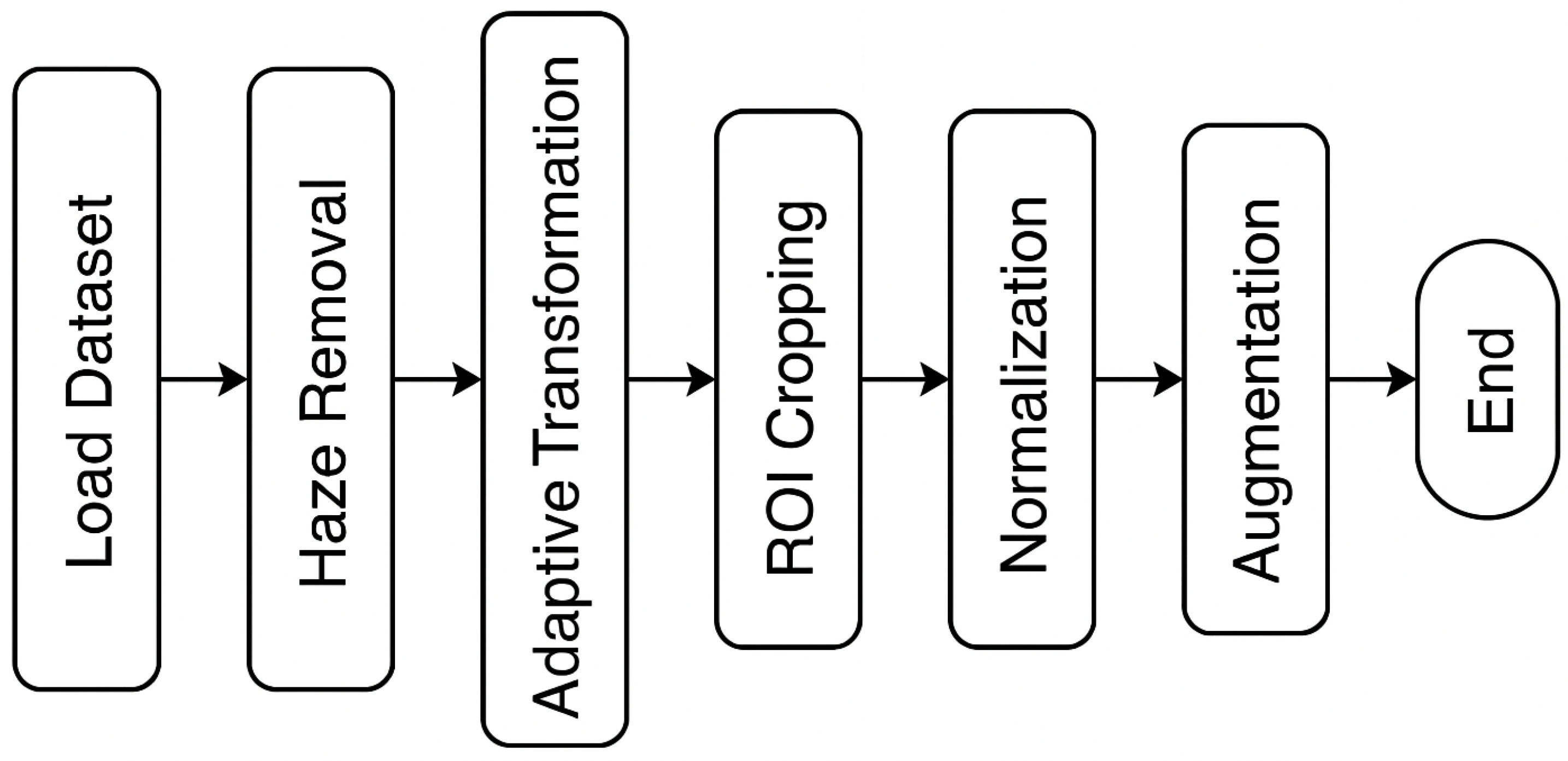
By generating more distinctive training dataset images, data augmentation has enhanced the model’s diversified feature-learning capabilities [41]. Deep learning generalizes effectively and performs well when there is a significant amount of learned data. Random variations are introduced during each optimization iteration through data augmentation. In order to preserve the integrity of the image, this was meticulously implemented during the augmentation process. Medical imaging datasets are considerably smaller. Consequently, the dataset is multiplied by the augmentation approach. This approach mitigates overfitting as a consequence of inadequate training data [42]. Consequently, we implemented database training samples to facilitate augmentation. The training images were improved using a variety of image processing techniques, such as rotation (−55° to 55°, step value of 5), flipping (vertical and horizontal), scaling (15°), Gaussian noise (mean zero, 0.25 variance), and gamma-correction (gamma from 0.2 to 1.5). Training photos from the augmented dataset increased by a factor of 30 in comparison to the original images. The MIAS, DDSM, and INbreast datasets contained 9000, 35,820, and 4380 training photos, respectively, after augmentation. The augmented data from the original dataset photos are summarized in

Table 4. Comparison of the original class sizes with augmented class sizes across each dataset.

Output Images	MIAS		DDSM		INbreast
	Original	Augmented	Original	Augmented	Original	Augmented
Malignant	39	1170	637	19,110	70	2100
Benign	52	1560	557	16,710	76	2280
Normal	209	6270	-	-	-	-

.

3.4. Preprocessing

In the datasets, all images’ fields of view (FOVs) and sizes were distinct; thus, image cropping was performed before the multi-parametric image analysis and training. The minimum margins of left, right, and top were set to 20, 20, and 40, respectively, during the cropping process for assurance of the presence of breast tissue in the middle of the image. Two groups were created from the cropped images according to the anatomy of breast names as left and right. To eliminate Gaussian noise from DWI images, a fast nonlocal means a denoising technique was utilized [43]. The bilinear interpolation on the dataset achieved a final size of $224\times 224$.

All input images were scaled to a uniform dimension of 224 × 224 pixels to ensure compatibility with the proposed CNN architecture. The standardization is essential as convolutional neural networks necessitate uniform input sizes to facilitate batch processing and provide consistent feature map dimensions throughout layers. Resizing enhances GPU memory utilization and promotes effective training. Before resizing, each image was cropped to focus on the region of interest (ROI) to maintain the pertinent diagnostic area, and enhancing techniques were employed to preserve essential visual qualities. This method mitigates spatial distortion and guarantees that tumor characteristics remain visually discernible in the enlarged images.

Pixel values were normalized through the z-scoring technique after cropping [44]. Since the number of slices was not constant among the different patients and image types, a nearest-neighbor resampling technique was employed to achieve a consistent 30 slices for each image type and case. Image cropping was performed using Python v3.13.2 and Scikit images v1.1. Though z-scoring and fast nonlocal denoising techniques were executed using Python and OpenCV (version 0.16.1), the complete preprocessing of available images was performed automatically. All images were obtained from the same session and position, so there was no need for co-registration of different sequences for this research. The output of cropping is shown in Figure 4.

3.5. Proposed CNN Model Architecture

To improve performance, the CNN model incorporates essential characteristics from U-Net and YOLO into its architecture. Like U-Net’s encoder, the feature extraction procedure uses multi-scale convolutions and residual connections to enhance classification accuracy instead of a symmetrical decoder. YOLO’s localization-inspired technique is modified to extract discriminative features from full photos rather than specific parts. The model treats mammography as a single analysis window instead of object detection to include all relevant regions. The input features are adjusted relative to the image size to represent uniform resolutions. This hybrid approach lets the model capture fine-grained spatial data while keeping global contextual information, making it ideal for mammographic picture categorization and interpretation. The 32-layer CNN model in Figure 5 optimizes deep learning for feature extraction and classification. Like ResNet architectures, it uses residual blocks with skip connections to improve gradient flow and prevent vanishing gradients. The residual blocks use $3\times 3$ and $5\times 5$ multi-kernel convolutions to capture fine-grained and larger spatial patterns in images. Batch normalization stabilizes training after each convolution, while ReLU activation ensures non-linearity in learning complicated representations. Stridden convolutions down-sample feature maps instead of max pooling, lowering computational complexity while maintaining spatial hierarchies. Using a $1\times 1$ convolution transition block refines feature maps before global average pooling, reducing the number of parameters and improving memory efficiency.

Dropout layers (0.3 probability) before fully linked layers minimize overfitting and ensure robustness and generalization across datasets. The model ends with a fully connected layer with 512 neurons and a softmax output layer to classify images into 10 categories. This architecture balances performance and efficiency, making it suited for applications with limited computational resources. Progressive depth filters (up to 512) allow the network to enhance its feature representations while retaining a reasonable memory footprint. This 32-layer CNN model uses residual learning, multi-kernel convolutions, and adaptive pooling to classify images accurately.

The proposed CNN model efficiently allocates and uses memory to optimize computational speed and parameters. There are 93,939,074 parameters or 358.35 MB of RAM. Convolutional, batch normalization, and fully linked layer weights and biases are trainable, and 93,907,202 parameters (358.23 MB) are changed during backpropagation. The 31,872 (124.50 KB) non-trainable parameters come from layers like batch normalization, where moving averages and variance statistics are kept apart from trainable weights. Deep residual connections, massive convolutional filters, and fully connected layers drive the memory footprint, with weight matrices and feature maps requiring significant storage. Due to its vast parameter space, this model requires GPU VRAM or system RAM for training. Mixed precision training, smaller batch sizes, and parameter pruning might reduce memory usage in resource-constrained contexts.

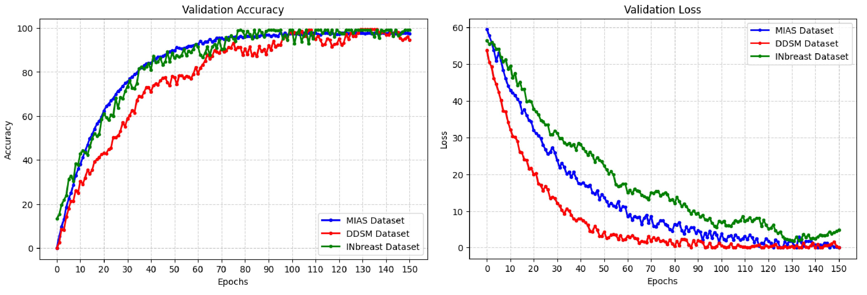
3.6. CNN Model Training

The proposed framework was trained using several cautiously performed processes executed on a local computer. A computer with the specification of Core i5, 13th Gen with 32 GB RAM, and RTX 3050 GPU was utilized to perform all experiments, which immensely helped the effectiveness and optimization of the proposed framework. Each dataset comprised randomly selected photos that were divided into training and testing sets by stratified selection to maintain the class distribution of malignant, benign, and normal samples. A 50–50 division was employed to guarantee an equitable assessment. The randomization procedure utilized a fixed seed to guarantee reproducibility across experiments. During the training process, a batch size of 32 was used; it was a very good decision that accelerated the robustness of the model’s parameters. Then, 150 epochs were utilized for the model training to understand better and adapt patterns and deep characteristics of the training dataset. The $1\times {10}^{-3}$ learning rate was used to achieve better stability. During the training step, this learning rate helped the framework escape from the harmful impacts on its equilibrium and continuously progress in learning the features. To select these optimum parameters, i.e., learning rate and batch size, many experiments were performed on different values and the best values were noticed for the proposed framework.

$$\mathrm{CEL}(l,l^{\prime })=-\sum _k{l}_k{log}_{10}\left(l_k^{\prime }\right)$$

(12)

$\mathrm{CEL}$ is the cross-entropy loss, l is the label distribution, l is the predicted label distribution, and k is the class iteration number.

$$\mathrm{MSE}(l,l^{\prime })={\displaystyle \frac{1}{K}}\sum _{k=1}^K{\left(l_k-l_k^{\prime }\right)}^2$$

(13)

MSE is the mean square error and K is the number of samples. We carefully used the cross-entropy loss and mean squared error (MSE) loss functions to optimize the suggested model. Both loss functions helped fine-tune the proposed model’s classification and localization capabilities. After this, to evaluate the overall performance of the framework, the separate losses of classification, and localization modules were added, to generate the combined loss. The suggested framework’s localization mechanism, inspired by YOLO, treats the entire image as a window. The datasets were augmented to align with this technique because x, y, and radius values were accurately divided by $512\times 51$2. The image size shows the dimensions of height and width.

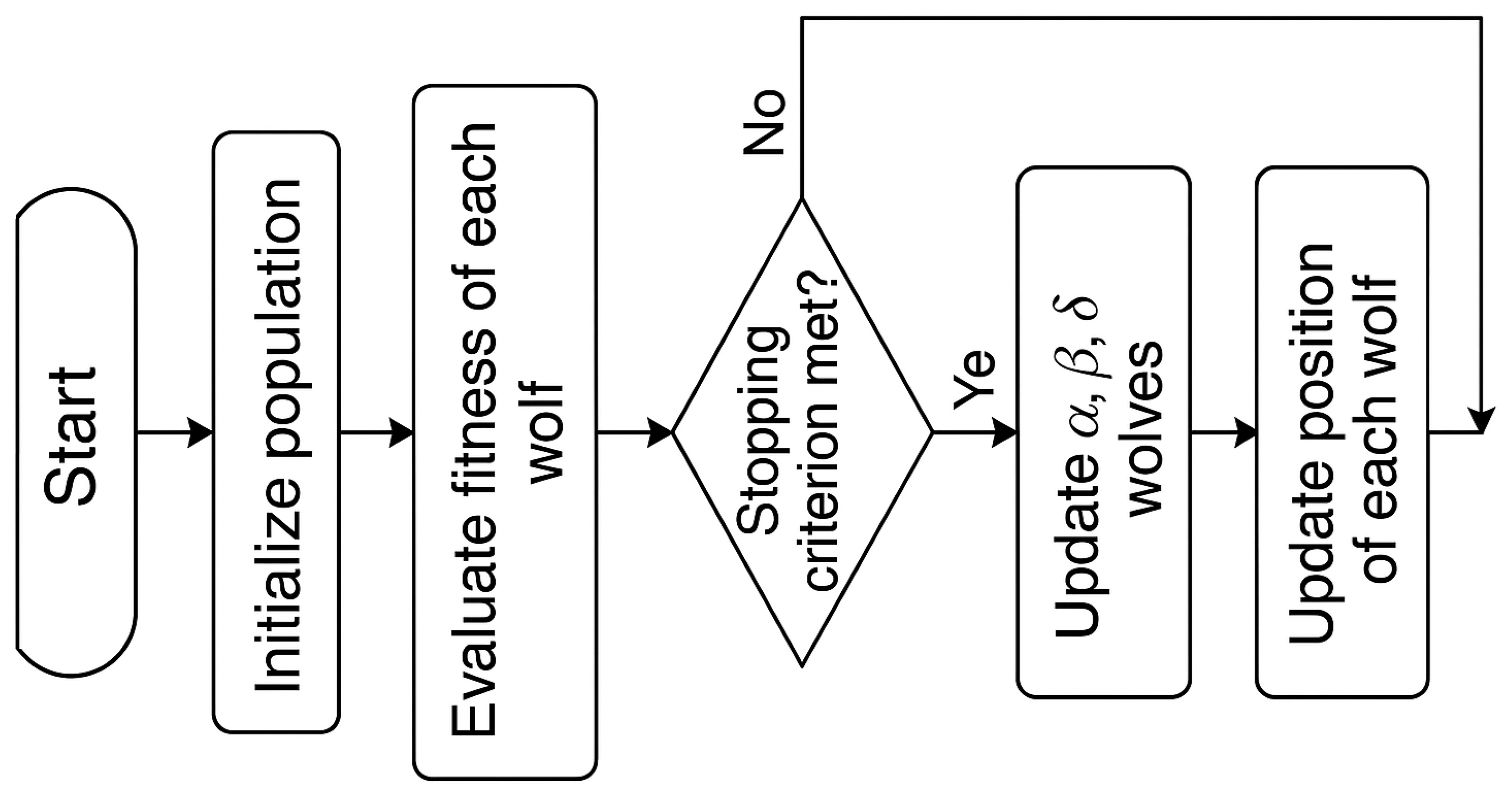
3.7. Modified Grey Wolf Optimization (mGWO) Algorithm

The Grey Wolf Optimization (GWO) algorithm is a Swarm Intelligence Algorithm inspired by nature [45]. The hunting and social leadership habits of grey wolves inspire it. The algorithm identifies x, y, and z as optimal solutions. The three wolves in command guide the remaining about the global optimum solution [46]. The GWO algorithm has presented a strategy for grey wolves’ leadership hierarchy and community living behavior. Grey wolves typically live in groups of 5 to 12. The group leader is x wolf, making significant decisions for the group. As a result, x wolves are called the dominating wolves, i.e., they order other wolves to follow whatever they say. The y wolves come second in command after the x wolf. They obey x wolf commands and come in command if the x wolf dies. The wolves z can hold numerous positions in the group, including scouts, elders, hunters, and caretakers. The x and y wolves primarily train the z wolves, but they also manage the $\alpha$ wolves, who are relatively low-ranking wolves and typically play the scapegoat role. They must follow the commands of x, y, and z wolves. They assist in resolving internal difficulties despite their lack of significance as wolves.

A three-step process helps the GWO optimizer to find an ideal solution efficiently. Encircling the prey begins with the optimizer initializing a search boundary around the best-known solution. The program can focus on promising search space regions. Second, hunting the prey involves exploration, where several candidate solutions modify their placements dynamically based on the top performers. This phase balances global and local searches to help the optimizer find optimal regions. In the third step, attacking the prey, the optimizer intensifies local alterations to refine the search for the optimum solution. Refinement of positional updates ensures convergence to an optimal or near-optimal solution. These three stages help the optimizer navigate complex search areas and optimize performance.

3.7.1. Encircling the Prey

The first step of GWO is to encircle the prey according to the following equations:

$$\begin{array}{c}\hfill N(i+1)=\left|M{P}_n\left(i\right)-P\left(i\right)\right|\\ \hfill P_n(i+1)=P_n\left(i\right)-L·N(i+1)\end{array}$$

(14)

$P_n$, P, and i denote the position of the prey, the position vector for grey wolf, and the iteration number. M and L are vectors of the coefficients.

$$\begin{array}{c}\hfill L=2·\phi \left(i\right)·a-\phi \left(i\right)\\ \hfill M=2·b\\ \hfill \phi \left(i\right)={\displaystyle \frac{2-2i}{N}}\end{array}$$

(15)

The values of random vectors a and b range from 0 to 1 that regulate the influence of each component on the ultimate fused feature score, and $\phi$ will decrease between 2 and 0 for the following values of i. Here, l and M refer to the scalar outputs (feature scores) derived from the pooling of their respective branches.

3.7.2. Hunting of Prey

x, y, and z are known as best hunter wolves as they know about the location of the prey. The behavior of hunting is described using the following equations:

$$\begin{array}{c}\hfill L=2·\phi \left(i\right)·a-\phi \left(i\right)\\ \hfill M=2·b\\ \hfill \phi \left(i\right)=2-{\displaystyle \frac{2i}{N}}\\ \hfill N_x=\left|M_1·P_x-P\left(i\right)\right|\\ \hfill N_y=\left|M_2·P_y-P\left(i\right)\right|\\ \hfill N_z=\left|M_3·P_z-P\left(i\right)\right|\\ \hfill P_{j1}\left(i\right)=P_x\left(i\right)-L_{j1}·N_x\left(i\right)\\ \hfill P_{j2}\left(i\right)=P_y\left(i\right)-L_{j2}·N_y\left(i\right)\\ \hfill P_{j3}\left(i\right)=P_z\left(i\right)-L_{j3}·N_z\left(i\right)\\ \hfill P(i+1)={\displaystyle \frac{P_{j1}\left(i\right)+P_{j2}\left(i\right)+P_{j3}\left(i\right)}{3}}\end{array}$$

(16)

$P_x$, $P_y$, and $P_z$ are the optimal solutions for the iterations $L_1$, $L_2$, and $L_3$. $a\in {[0,1]}^n$ is a random vector controlling the adaptive scaling of step sizes during exploration; $b\in {[0,1]}^n$ is a random vector controlling the stochastic influence during movement updates; $\phi \left(i\right)$ is a control parameter linearly decreasing from 2 to 0 over iterations, regulating the transition from exploration to exploitation; and L and M are coefficient vectors calculated using a, b, and $\phi \left(i\right)$ to modulate the directional search pressure from the three best wolves ($\alpha$, $\beta$, $\delta$). By taking into account the relative distance of each wolf from the top three candidates, these terms collectively guarantee that the position of each wolf in the population is updated, thereby improving both local refinement and global search.

3.7.3. Attacking of Prey

The hunting phase ends when the prey stops moving, and the wolves start attacking. This is carried out because the value of $\phi$ will begin to drop in the subsequent iterations; $\phi$ also controls how grey wolves explore and exploit their prey. Exploration takes up about half of the iterations with a seamless transition, while exploitation takes up the other half. Wolves randomly switch between their current location and the position of the prey. This approach randomly creates wolves in the search space. Wolf positions are determined by the objective function. The steps are repeated until the halting condition or preset number of iterations is reached. In each iteration, x, y, and z are the first three wolves with the best fitness. The wolves adjust their positions based on the earlier hunting, attacking, and encircling steps. Consequently, the optimal prey location, the x’s position, can be identified.

3.7.4. Objective Function

The objective function for GWO, WOA, and the hybrid algorithm of GWO and WOA is the Rastrigin function. To direct the mGWO algorithm in feature selection, we establish a composite fitness function that assesses each feature subset according to two criteria: (1) the classification error rate and (2) the ratio of selected features to the total number of accessible features. This trade-off guarantees that the algorithm prioritizes feature subsets that achieve high classification accuracy while simultaneously being compact and computationally economical. The fitness function is articulated as follows:

$$F=\alpha ·{\displaystyle \frac{E_{cls}}{E_{max}}}+(1+\alpha )·{\displaystyle \frac{N_{sel}}{N_{total}}}$$

(17)

Here, $E_{cls}$ represents the classification error $(1-accuracy)$ of the feature subset assessed using the CNN classifier, $N_{sel}$ is the number of selected features, and $N_{total}$ indicates the total number of features prior to selection. E max represents the maximum permissible error (i.e., 1.0), utilized for normalization purposes. The parameter $\alpha \in [0,1]$ serves as a weighting factor that regulates the equilibrium between classification accuracy and feature compactness. In our trials, we established $\alpha =0.8$ to emphasize classification efficacy while simultaneously promoting dimensionality reduction. The optimization procedure seeks to decrease this fitness function. Subsets that produce reduced classification error and fewer features will result in a diminished fitness value, hence being preferred by the mGWO algorithm. Figure 6 illustrate the trade-off between accuracy and feature count during optimization.

Optimization method performance testing uses the Rastrigin function and non-linear multimodal function. Several local minima exist in the function. Optimization algorithms must be run from many starting points. One global minimum exists for this function, and all local minimums are higher. Due to early convergence, GWO might get stuck in local minima. To solve this problem, multimodal functions can be used to evaluate the algorithm’s ability to avoid local minima and attain global minima. As previously explained, GWO is a widely used metaheuristic optimization algorithm inspired by grey wolf social hunting behavior. Despite its effectiveness, GWO suffers from premature convergence, lack of diversity in the search process, and suboptimal exploration–exploitation balance. In this study, we propose three modifications to improve GWO and prove mathematically that these enhancements improve its overall performance.

3.8. Modifications in GWO

3.8.1. Modification I—Adaptive Dynamic Parameter Control for Exploration and Exploitation

The exploration and exploitation phases of GWO are controlled by the coefficient $\phi \left(i\right)$, which linearly decreases from 2 to 0 as the algorithm progresses. This fixed decay rate may lead to slow exploration in early iterations and premature convergence in later iterations due to rapid exploitation. In standard GWO, the coefficient $\phi \left(i\right)$ is updated as Equation (7). This linear decay limits early exploration. Toward the end, the search agents become too static, reducing the probability of escaping local optima. To improve this, we propose a non-linear decay function for AAA instead of the traditional linear decrease:

$$\phi \left(i\right)=2\times e^{-\mathit{\partial }\times \left({\displaystyle \frac{i}{N}}\right)}$$

(18)

where ∂ is a decay factor (typically 3), and $e^{-\mathit{\partial }\times \left({\displaystyle \frac{i}{N}}\right)}$ ensures a slower and faster decay. This allows more aggressive exploration in the early stages while ensuring fine-tuned exploitation toward convergence. The non-linear decay ensures that $\phi \left(i\right)$ remains higher for longer, allowing the search agents to explore a more extensive search space. In standard GWO, $\phi \left(i\right)$ decays linearly, leading to a constant exploration–exploitation shift, whereas in modified GWO, $\phi \left(i\right)$ follows an exponential decay, ensuring extended exploration before convergence.

The decay factor ∂ in the non-linear attenuation function is essential for regulating the shift from exploration to exploitation in the modified GWO. A reduced ∂ leads to a more gradual decline of the control parameter $\phi \left(i\right)$, thereby prolonging the exploration of a wider search space. Conversely, a greater ∂ results in a more rapid decline in $\phi \left(i\right)$, promoting early exploitation while heightening the risk of premature convergence. To ascertain an appropriate value for ∂, we performed an ablation research utilizing the MIAS dataset, assessing ∂ values ranging from $1.0$–$5.0$ in increments of 0.5. The findings indicated that when ∂ $= 1.0$–$2.0$, the decay was excessively gradual, resulting in extended exploration, delayed convergence, and increased variance in outcomes. If ∂ $= 4.0$–$5.0$, the decay was excessively steep, favoring premature exploitation, which frequently resulted in early convergence and suboptimal feature subsets. Conversely, if ∂ $= 3.0$, this value offered the optimal balance, facilitating adequate exploration in initial iterations while ensuring effective convergence in subsequent iterations. Following this empirical study, we chose ∂ $= 3.0$ for all our studies. This decision allowed the algorithm to preserve variation within the population throughout the early optimization phases and to consistently converge on high-performing feature subsets in the later iterations.

3.8.2. Modification II—Chaos-Based Position Update for Better Global Search

In traditional GWO, wolf positions are updated using the weighted average of alpha ($\alpha$), beta ($\beta$), and delta ($\delta$) wolves, which may cause early convergence and stagnation in local optima. The standard update equations are Equation (6). These deterministic equations lack stochastic elements, making the search process predictable. We introduce Chaotic Sequences using the logistic map, which introduces randomness into the search process:

$$\begin{array}{c}\hfill N(i+1)=4\times N(i+1)\times \left(1-N(i+1)\right)\\ \hfill P_n(i+1)=\left(P_{\alpha }-\phi \left(i\right)\right)\times N_{\beta }+N(i+1)\times \left(P_{\delta }-P_{\beta }\right)\end{array}$$

(19)

This enhances exploration by introducing a random perturbation between delta $P_{\delta }$ and beta $P_{\beta }$. Here, chaos adds randomness, avoiding premature convergence. Meanwhile, it retains the balance between the best wolves and introduces stochastic elements, which increases global search efficiency. In parallel, the logistic map ensures unpredictable updates, making it difficult for wolves to stagnate in local minima. Thus, chaos-based updates introduce a dynamic exploration strategy into GWO, providing a higher probability of reaching the global optimum. The logistic map exhibits chaotic behavior when the control parameter is set to 4 (fully chaotic regime) and the initial value $N\left(0\right)\in (0,1)$, excluding fixed points like 0.25, 0.5, or 0.75.

3.8.3. Modification III—Opposition-Based Learning (OBL) for Faster Convergence

GWO starts with a random initial population, with random positions, which may be far from the optimal solution. If the initial wolves are poorly placed, the algorithm spends more iterations just improving bad solutions, leading to slow convergence. We incorporate opposition-based learning (OBL), where we generate opposite solutions to complement the randomly initialized ones:

$$P_{\mathrm{Opp}}=P_{\min }+P_{\max }-P$$

(20)

If the fitness of $P_{\mathrm{Opp}}$ is better than P, we replace P with $P_{\mathrm{Opp}}$. The advantages of doing so is that (a) it expands the initial search space by considering opposite solutions, (b) doubles the probability of initializing closer to the global optimum, and (c) improves the convergence speed since better solutions are discovered earlier. Thus, using OBL, the algorithm is more likely to start near the optimal solution, leading to faster convergence rates. Due to deterministic position updates, the original GWO has a convergence complexity of $O\left(nlogn\right)$. By integrating adaptive parameter control to increase search space coverage, chaos-based updates to enhance global search, and opposition-based learning to ensure better initial solutions, the modified GWO mathematically improves search efficiency, reducing O’s complexity $\left(n\right)$. The parameters for the mGWO are given in

Table 5. Parameters and their values adopted for mGWO in this work.

Parameters	Values
Iterations (n)	100 or multiples of 100 s
Population	5 or multiples of 5 s
Total Features	65
Total Instances	646
Upper Bound	100
Lower Bound	−100
Control Parameter	Linear decrement from 2 to 0

, whereas overall flow of HRAT is shown in Figure 7.

Consider a simple binary feature selection problem with five features $[f_1,f_2,f_3,f_4,f_5]$. We initialize a population of three wolves (solutions), each represented as a binary string indicating selected features as $WolfA\left(Alpha\right):[1,0,1,1,0]\to selects features 1,3,4$; $WolfB\left(Beta\right):[0,1,1,0,1]\to selects features 2,3,5$; and $WolfC\left(Delta\right):[1,1,0,1,0]\to selects features 1,2,4$. Each solution is evaluated using a fitness function that balances classification accuracy and the number of selected features:

$$Fitness=\alpha ·Erro{r}_{cls}+(1-\alpha )·{\displaystyle \frac{N_{sel}}{N_{total}}}$$

(21)

Assume the fitness values for these wolves are Alpha 0.32, Beta 0.41, and Delta 0.39 (lower is better). The positions (feature sets) of the remaining wolves are updated using the enhanced mGWO strategy, which incorporates a chaotic map to diversify search directions and opposition-based learning to reverse weak solutions and explore better regions. For instance, a chaotic adjustment to Wolf B might produce $[1,1,1,0,0]$, selecting features 1, 2, 3—a potentially better subset. This new candidate is then evaluated, and the leaders are updated accordingly. Over iterations, the population converges toward an optimal feature subset that achieves high classification accuracy with minimal redundancy.

4. Experimental Results

4.1. Experimental Setup

In order to prevent overfitting, this investigation assesses both the current and proposed models through the use of 5-fold cross-validation (CV). The dataset is partitioned into five folds to ensure a similar class distribution. Each experiment involves the testing of one fold and the subsequent training of the remaining folds. To guarantee the generality and stability of the model, the 5-fold CV was executed ten times.

Table 6. Hyperparameter values to train the proposed model.

Hyperparameter	Value
L2 regularization	0.0001
Initial learning rate	0.001
Momentum	0.7
Total epochs	150
Batch size	32
Data split ratio	50–50

contains the optimal hyperparameters for the proposed CNN model, as determined by experimental tuning during training. Throughout the transfer learning process, the SGDM technique employs identical hyperparameters for 100 epochs.

To assess the quality and impact of the enhancement process, we computed two critical image quality metrics: mean squared error (MSE) and entropy. The level of information and contrast in the image is reflected in entropy; higher entropy values imply a more effective enhancement of fine details, which is essential for the visualization of tumor boundaries. MSE, in contrast, quantifies the extent to which the enhanced image deviates from the original, thereby offering a measure of the degree of distortion or noise that may have been introduced during the processing process. The HRAT method’s efficacy in enhancing image interpretability while maintaining diagnostic integrity is evaluated through a collaborative analysis of these metrics.

4.2. Results and Analysis

The efficacy of the customized CNN model, as demonstrated by critical metrics, is illustrated in this section. Accuracy, specificity, precision, r-squared error, F1-score, and Kappa were the eight performance metrics that were employed to evaluate the proposed model. Our model’s accuracy was confirmed by employing the 5-fold CV approach on ten occasions during the initial experiment. The model was able to comprehend high-level features by manually specifying hyperparameters in each fold. Over ten iterations and five configurations, the proposed model showed strong and consistent classification accuracy. Results show accuracy from 96.36% to 98.35%, with the most outstanding individual accuracy at 99.37%. The model works well across configurations, with $K=2$ and $K=3$ often extracting features more accurately. Its 97.74% accuracy and 1.04 standard deviation confirm the model’s robustness and generalization. Data distribution, model optimization, and training conditions may affect accuracy across iterations.

Table 7. Average classification accuracy of the proposed model on the MIAS dataset.

Iteration	$\mathit{K}=1$	$\mathit{K}=2$	$\mathit{K}=3$	$\mathit{K}=4$	$\mathit{K}=5$	Average Accuracy (%)
1	98.22 ± 0.95	99.27 ± 1.21	99.37 ± 1.18	96.75 ± 0.61	97.24 ± 0.83	98.16 ± 0.82
2	98.23 ± 1.04	97.63 ± 1.46	99.04 ± 1.32	97.85 ± 1.22	99.01 ± 1.08	98.35 ± 1.35
3	96.83 ± 1.01	97.89 ± 1.26	96.93 ± 0.59	96.77 ± 1.16	96.62 ± 1.46	96.99 ± 0.64
4	97.09 ± 1.21	95.89 ± 0.96	96.52 ± 1.16	96.39 ± 0.74	95.93 ± 1.24	96.36 ± 1.16
5	96.42 ± 1.31	99.16 ± 0.69	96.31 ± 1.06	97.93 ± 0.82	97.35 ± 1.14	97.42 ± 0.65
6	96.12 ± 1.32	98.33 ± 1.47	96.23 ± 1.18	97.44 ± 1.49	95.82 ± 0.83	96.78 ± 0.58
7	97.79 ± 1.23	96.48 ± 1.31	97.22 ± 1.33	97.68 ± 1.23	96.59 ± 1.41	97.15 ± 0.69
8	98.28 ± 1.17	97.11 ± 1.37	99.23 ± 0.56	95.86 ± 0.98	95.86 ± 1.06	97.27 ± 1.37
9	95.82 ± 0.59	97.08 ± 0.87	97.14 ± 1.35	96.88 ± 1.25	95.97 ± 1.22	96.58 ± 1.32
10	96.76 ± 0.55	96.86 ± 1.49	99.05 ± 0.96	96.63 ± 1.41	98.31 ± 1.02	97.52 ± 1.46
Overall Result	97.74 ± 1.04

shows that the proposed model regularly achieves excellent classification accuracy, making it a reliable solution for medical image analysis using the MIAS dataset.

Ten iterations and five configurations of the proposed model on the DDSM dataset yielded good classification accuracy. Individual accuracy ranges from 98.04 to 98.91%, with the highest at 99.37%. The model performs reliably across several settings, with K equals one and K equals four often producing superior accuracy, showing feature learning success. The model’s 99.37% accuracy and 0.19 standard deviation demonstrate its resilience and generalization. Slight fluctuation exists between iterations, indicating the model’s stability in medical image classification.

Table 8. Average classification accuracy of the proposed model on the DDSM dataset.

Iteration	$\mathit{K}=1$	$\mathit{K}=2$	$\mathit{K}=3$	$\mathit{K}=4$	$\mathit{K}=5$	Average Accuracy (%)
1	98.33 ± 0.52	98.81 ± 0.33	98.19 ± 0.99	98.76 ± 0.37	98.47 ± 0.69	98.91 ± 0.07
2	98.40 ± 1.18	98.23 ± 0.27	98.14 ± 0.03	98.24 ± 0.19	98.87 ± 0.85	98.18 ± 0.98
3	98.89 ± 0.68	98.41 ± 0.06	98.35 ± 0.57	97.76 ± 0.43	98.13 ± 0.81	98.29 ± 0.29
4	98.34 ± 0.52	98.38 ± 0.09	98.36 ± 0.51	98.93 ± 0.08	98.37 ± 0.34	98.88 ± 0.79
5	97.90 ± 0.41	98.37 ± 0.68	98.85 ± 0.56	98.14 ± 0.57	98.43 ± 0.63	98.54 ± 0.47
6	98.08 ± 0.09	98.05 ± 0.22	98.17 ± 0.95	98.16 ± 0.36	98.32 ± 0.65	98.34 ± 0.86
7	98.39 ± 0.67	98.60 ± 0.10	97.83 ± 0.08	98.55 ± 0.07	98.02 ± 0.65	98.88 ± 0.72
8	98.57 ± 0.57	98.71 ± 0.07	98.73 ± 0.89	98.64 ± 0.75	98.56 ± 0.74	98.04 ± 0.65
9	98.22 ± 0.11	98.96 ± 0.88	98.16 ± 0.96	98.22 ± 0.38	98.16 ± 0.62	98.14 ± 0.52
10	98.71 ± 0.13	98.49 ± 0.78	98.27 ± 0.74	98.65 ± 0.73	98.87 ± 0.71	98.88 ± 0.73
Overall Result	99.37 ± 0.19

shows that the proposed model performs well on the DDSM dataset, making it appropriate for automated mammographic image processing.

On the INbreast dataset, the proposed model shows substantial classification accuracy throughout ten iterations and five configurations. Overall accuracy ranges from 97.17% to 98.81%, with the highest individual accuracy being 99.02%. The model performs well, with $K=1$ and $K=4$ often reaching greater accuracy, suggesting feature extraction and classification. The model’s 99.02% accuracy and 0.19 standard deviation demonstrate its stability and ability to generalize across mammographic images. Slight fluctuation is seen across iterations, indicating the model’s stability in medical image classification.

Table 9. Average classification accuracy of the proposed model on the INbreast dataset.

Iteration	$\mathit{K}=1$	$\mathit{K}=2$	$\mathit{K}=3$	$\mathit{K}=4$	$\mathit{K}=5$	Average Accuracy (%)
1	98.51 ± 1.07	98.51 ± 1.43	98.52 ± 0.85	97.25 ± 1.4	97.28 ± 0.67	98.73 ± 1.41
2	98.45 ± 0.89	98.16 ± 1.34	97.13 ± 1.01	98.85 ± 0.53	98.67 ± 1.38	98.45 ± 0.75
3	98.52 ± 0.84	98.77 ± 0.61	97.46 ± 0.75	97.96 ± 1.2	97.52 ± 1.31	97.25 ± 1.48
4	98.77 ± 1.41	97.42 ± 1.26	97.49 ± 0.96	97.02 ± 0.55	98.21 ± 0.58	97.98 ± 1.48
5	98.58 ± 1.22	97.01 ± 0.8	98.46 ± 0.77	98.54 ± 1.38	97.27 ± 1.37	97.56 ± 1.42
6	97.28 ± 0.78	97.42 ± 0.75	98.31 ± 0.53	98.01 ± 1.34	97.32 ± 0.62	97.66 ± 1.23
7	97.39 ± 1.09	97.35 ± 0.64	97.99 ± 0.88	97.91 ± 1.33	97.19 ± 1.47	97.17 ± 0.96
8	97.09 ± 0.58	97.69 ± 1.17	97.88 ± 0.95	97.72 ± 0.94	98.66 ± 0.93	98.81 ± 1.15
9	97.38 ± 0.96	97.92 ± 0.84	97.03 ± 0.61	97.18 ± 0.92	97.74 ± 0.67	97.45 ± 0.62
10	97.74 ± 0.55	97.44 ± 0.66	97.22 ± 0.52	97.09 ± 1.25	97.43 ± 0.83	97.18 ± 1.49
Overall Result	99.02 ± 0.19

shows that the proposed model accurately classifies INbreast dataset images, proving its usefulness for breast cancer detection and mammographic image processing. The confusion matrices for all datasets using the augmented data are shown in Figure 8.

4.3. Ablation Studies

Table 10. Comparison of pre-trained CNN models with the proposed model across all three selected datasets.

Model	Accuracy (%)	Sensitivity (%)	Specificity (%)	Precision (%)	RSE (%)	F1 (%)	Kappa (%)
MIAS dataset
VGG19	92.54 ± 1.04	93.67 ± 1.68	92.14 ± 1.47	93.74 ± 1.75	93.42 ± 0.91	93.58 ± 1.32	92.15 ± 0.56
ResNet50	95.02 ± 0.97	94.82 ± 0.64	93.69 ± 1.10	93.94 ± 1.06	93.74 ± 1.75	94.26 ± 1.27	94.21 ± 0.21
InceptionResNet-V2	95.85 ± 1.14	94.22 ± 1.28	96.75 ± 0.24	96.46 ± 0.53	95.04 ± 0.99	94.06 ± 0.07	94.78 ± 0.79
EfficientNet-B4	95.28 ± 0.67	92.56 ± 0.75	94.75 ± 0.82	95.11 ± 0.12	96.71 ± 0.97	95.86 ± 0.82	92.91 ± 1.19
Proposed Model	97.74 ± 1.04	98.02 ± 0.87	98.47 ± 0.97	98.79 ± 1.02	97.51 ± 0.76	94.94 ± 1.71	99.15 ± 0.84
DDSM dataset
VGG19	92.33 ± 0.66	91.17 ± 0.18	90.59 ± 0.63	91.61 ± 0.75	91.72 ± 1.13	90.67 ± 0.78	91.95 ± 1.04
ResNet50	92.07 ± 0.50	90.56 ± 0.79	94.38 ± 1.61	94.02 ± 1.03	94.64 ± 1.26	92.71 ± 0.58	92.97 ± 1.02
InceptionResNet-V2	92.91 ± 0.92	92.57 ± 0.61	91.91 ± 0.92	92.47 ± 0.48	92.74 ± 0.89	91.41 ± 3.42	92.05 ± 0.74
EfficientNet-B4	94.08 ± 1.45	93.87 ± 0.88	95.96 ± 0.03	92.82 ± 0.27	95.04 ± 0.86	94.75 ± 0.57	94.68 ± 1.26
Proposed Model	99.37 ± 0.19	97.98 ± 0.99	96.88 ± 1.89	98.36 ± 1.12	97.86 ± 1.87	99.05 ± 0.81	97.36 ± 0.31
INbreast dataset
VGG19	90.34 ± 0.84	89.06 ± 1.13	88.97 ± 0.98	88.63 ± 1.04	88.22 ± 0.94	88.84 ± 0.74	88.15 ± 1.16
ResNet50	89.21 ± 0.22	89.85 ± 2.86	91.42 ± 0.59	89.67 ± 1.61	89.78 ± 0.92	90.33 ± 0.74	89.27 ± 1.28
InceptionResNet-V2	88.44 ± 0.45	88.96 ± 1.97	88.81 ± 0.94	88.48 ± 0.49	88.98 ± 2.99	88.97 ± 1.98	90.07 ± 0.92
EfficientNet-B4	91.45 ± 0.46	93.15 ± 0.84	91.94 ± 0.95	91.77 ± 0.78	91.07 ± 2.08	92.75 ± 0.94	92.35 ± 0.82
Proposed Model	99.02 ± 0.19	99.86 ± 0.13	97.97 ± 1.98	98.08 ± 0.75	97.72 ± 1.41	98.16 ± 0.17	98.97 ± 0.75

compares the proposed model to pre-trained CNN models VGG19 [47], ResNet50 [48], InceptionResNet-V2 [49], and EfficientNet-B4 [50] on MIAS, DDSM, and INbreast. Accuracy, sensitivity, specificity, precision, relative standard error, F1-score, and Kappa score are evaluated. The proposed model beats all pre-trained models in all three datasets, with the highest classification accuracy and best evaluation metrics. The proposed model outperforms VGG19 at 92.54%, ResNet50 at 95.02%, and InceptionResNet-V2 at 95.85% on the MIAS dataset at 97.74%. The model has the highest sensitivity, specificity, and accuracy, proving it can better detect and categorize mammographic abnormalities. On the DDSM dataset, the proposed model obtains 99.37% accuracy, while the best pre-trained model, EfficientNet-B4, scores 94.08%, demonstrating a significant improvement. The proposed model outperforms EfficientNet-B4 with 99.02% accuracy on the INbreast dataset, which has 91.45%. The proposed model’s Kappa score, F1-score, and precision consistently increase, confirming its mammographic image classification reliability and resilience. The results show that the proposed model outperforms pre-trained CNNs for breast cancer detection and classification.

Table 11. Comparison of pre-trained CNN models with proposed model before and after image enhancement with mGWO across all three selected datasets.

Model	Image Enhancement		Dataset
	No	Yes	MIAS	DDSM	INbreast
VGG19	✓	×	91.94 ± 1.47	90.83 ± 0.93	90.63 ± 1.52
	×	✓	92.54 ± 1.04	92.33 ± 0.66	90.34 ± 0.84
ResNet50	✓	×	92.15 ± 0.57	91.11 ± 0.35	93.41 ± 0.63
	×	✓	95.02 ± 0.97	92.07 ± 0.50	89.21 ± 0.22
InceptionResNet-V2	✓	×	90.68 ± 0.97	89.15 ± 0.24	84.22 ± 1.27
	×	✓	95.85 ± 1.14	92.91 ± 0.92	88.44 ± 0.45
EfficientNet-B4	✓	×	89.98 ± 1.24	89.09 ± 0.17	86.41 ± 0.51
	×	✓	95.28 ± 0.67	94.08 ± 1.45	91.45 ± 0.46
Proposed Model	✓	×	93.55 ± 1.10	94.36 ± 1.21	93.86 ± 1.47
	×	✓	97.74 ± 1.04	99.37 ± 0.19	99.02 ± 0.19

compares pre-trained CNN models and the proposed model before and after image augmentation using MIAS, DDSM, and INbreast benchmark datasets. Image enhancement enhances classification performance for all models, with the proposed model having the highest accuracy across all datasets. Image enhancement increases VGG19’s accuracy from 91.94% to 92.54%, ResNet50’s from 92.15% to 95.02%, and EfficientNet-B4’s from 89.98% to 95.28% on the MIAS dataset. The proposed model outperforms all pre-trained models with 97.74% accuracy, up from 93.55% without improvement. In the DDSM dataset, VGG19, ResNet50, and EfficientNet-B4 improve slightly after image improvement, but the proposed model achieves exceptional accuracy of 99.37%, up from 94.36%. Image enhancement enhances performance in the INbreast dataset, with the proposed model achieving 99.02% accuracy from 93.86%, whereas other pre-trained models improve less. This illustrates that image improvement is vital to boosting mammographic image classification accuracy, especially for the proposed model, which benefits the most across all datasets. Feature visibility, noise reduction, and contrast improve performance, allowing the model to extract more discriminative features for exact classification. The comparison also shows that the proposed model beats pre-trained CNNs before and after image augmentation, giving it a more reliable breast cancer detection and classification solution.

Table 12. Comparison of pre-trained CNN models with proposed model before optimization, with GWO and with mGWO before image enhancement across all three selected datasets.

Model	Feature Optimization			MIAS Dataset	DDSM Dataset	INbreast Dataset
	No	GWO	mGWO
VGG19	✓	×	×	85.13 ± 0.93	87.76 ± 1.12	86.22 ± 1.23
	×	✓	×	89.64 ± 1.48	89.02 ± 0.55	97.95 ± 1.34
	×	×	✓	87.54 ± 1.04	86.33 ± 0.66	88.34 ± 0.84
ResNet50	✓	×	×	86.60 ± 0.61	87.06 ± 1.42	86.99 ± 1.46
	×	✓	×	90.24 ± 1.05	91.07 ± 0.53	91.23 ± 1.21
	×	×	✓	95.02 ± 0.97	92.07 ± 0.50	89.21 ± 0.22
InceptionResNet-V2	✓	×	×	87.15 ± 0.61	87.89 ± 0.08	88.16 ± 0.05
	×	✓	×	92.16 ± 0.87	92.94 ± 0.05	91.69 ± 1.29
	×	×	✓	95.85 ± 1.14	92.91 ± 0.92	88.44 ± 0.45
EfficientNet-B4	✓	×	×	90.26 ± 1.24	89.77 ± 0.96	89.06 ± 1.24
	×	✓	×	93.79 ± 0.81	92.12 ± 1.12	93.46 ± 0.72
	×	×	✓	95.28 ± 0.67	94.08 ± 1.45	91.45 ± 0.46
Proposed Model	✓	×	×	92.05 ± 1.57	91.78 ± 1.44	90.51 ± 1.17
	×	✓	×	93.92 ± 0.42	94.01 ± 0.92	94.34 ± 0.79
	×	×	✓	97.74 ± 1.04	99.37 ± 0.19	99.02 ± 0.19

compares pre-trained CNN models and the proposed model before and after feature optimization using GWO and mGWO on the MIAS, DDSM, and INbreast datasets. Features optimization improves classification performance, with the proposed model having the highest accuracy across all datasets after mGWO optimization. GWO improves VGG19, ResNet50, and EfficientNet-B4 accuracy on the MIAS dataset from 85.13% to 89.64%, 86.60% to 90.24%, and 90.26% to 93.79%. After optimization, the proposed model’s accuracy rises to 93.92% with GWO and 97.74% with mGWO, surpassing all previous models. In the DDSM dataset, VGG19, ResNet50, and EfficientNet-B4 improve moderately after GWO and mGWO, but the proposed model reaches 99.37% after mGWO optimization, up from 91.78% without optimization. The proposed model achieves 99.02% after mGWO in the INbreast dataset, up from 90.51% before optimization. All datasets show that mGWO improves classification accuracy more than traditional GWO. The validation accuracy and loss of propsoed model is shown in Figure 9, whereas the receiver operating characteristic (ROC) curves of all three datasets for proposed model are shown in Figure 10.

Altering the dataset significantly affects the model’s behavior and the attributes of the chosen images. Datasets like MIAS, DDSM, and INbreast vary in image quality, resolution, annotation criteria, and class distributions. These disparities influence feature distribution and the complexity of classification. The choice of image samples can also affect the outcomes, especially when dealing with small datasets or imbalanced class distribution. To resolve this, we utilized stratified random sampling to guarantee that the training and testing sets preserve class equilibrium. To assess the generalizability of the proposed framework, we performed separate experiments on each dataset. Table 7, Table 8 and Table 9 illustrate that performance metrics exhibit minor variations among datasets, indicating that although the model demonstrates adaptability, the foundational dataset influences learning results. This underscores the significance of testing across varied datasets.

4.4. Comparison of mGWO with State-of-the-Art Optimization Algorithms

Particle Swarm Optimization (PSO) [51] simulates bird and fish social behavior by moving particles within a search area influenced by their personal and global best placements. This enables quick convergence in continuous optimization problems. Ant Colony Optimization (ACO) [52] uses pheromone trails to probabilistically lead search agents inspired by ant foraging behavior, making it perfect for combinatorial issues like routing and scheduling. The Bat Algorithm (BA) [53] uses echolocation to balance exploration and exploitation by altering frequency, loudness, and pulse rate. This needs careful parameter tuning to prevent local optima. Cuckoo Search Algorithm (CSA) [54] replicates brood parasitism by using Lévy flights to introduce big jumps for global search, improving exploration but increasing computational cost. The Whale Optimization Algorithm (WOA) [55] simulates humpback whale bubble-net hunting employing spiral updating and encircling methods to improve search efficiency, performing well in multimodal functions.

Table 13. Comparison in terms on accuracy of different state-of-the-art optimization algorithms with mGWO.

Optimization Algorithm	MIAS Dataset	DDSM Dataset	INbreast Dataset
PSO	82.58 ± 1.32	83.42 ± 1.39	83.63 ± 1.36
ACO	86.64 ± 0.57	89.41 ± 1.40	90.53 ± 1.29
BA	88.23 ± 0.51	91.71 ± 0.67	90.41 ± 1.07
CSA	81.69 ± 0.54	85.67 ± 1.30	84.46 ± 0.54
WOA	89.08 ± 1.28	91.18 ± 1.44	92.38 ± 1.17
GWO	93.92 ± 0.42	94.01 ± 0.92	94.34 ± 0.79
mGWO	97.74 ± 1.04	99.37 ± 0.19	99.02 ± 0.19

compares state-of-the-art feature selection optimization algorithms, including PSO, ACO, BA, CSA, WOA, GWO, and mGWO, across the MIAS, DDSM, and INbreast datasets. Across all three datasets, mGWO exceeds all other optimization methods in classification accuracy. PSO accuracy for the MIAS dataset is 82.58%, ACO 86.64%, BA 88.23%, and WOA 89.08%. GWO increases accuracy to 93.92%, whereas mGWO provides the most significant improvement at 97.74%. Similarly, in the DDSM dataset, PSO and CSA perform poorest with 83.42% and 85.67%, whereas GWO obtains 94.01% and mGWO exceeds all with 99.37%. PSO and CSA performed worst in the INbreast dataset, whereas mGWO performed best at 99.02%, surpassing WOA at 92.38% and GWO at 94.34%. These results show that mGWO is all datasets’ best feature selection and classification optimization method. Better exploration and exploitation, adaptive weight modifications, and convergence speed boost mGWO performance. The comparison also shows that GWO and its modified version beat standard optimization methods in accuracy. The results show that the mGWO optimization strategy improves breast cancer detection classification performance most reliably and efficiently.

Figure 11 shows how well Grad-CAM and LIME, two popular explainability methods, extract and optimize the proposed model’s features. The first row (Image with Mask) shows the original mammographic pictures with bounding boxes emphasizing ground truth lesion spots. The categorization technique identified these sites as potentially cancerous or suspicious. The model’s feature activation zones are visualized using Gradient-weighted Class Activation Mapping in the second row. This method reveals the model’s spatial importance by highlighting the categorization decision’s most important locations. Warm colors (yellow and red) over lesion sites suggest that the 32-layer CNN model, improved with mGWO for feature optimization, correctly concentrates on key mammographic regions, exhibiting its good localization capabilities. Third row (LIME visualization) validates model interpretability and feature importance with Local Interpretable Model-Agnostic Explanations (LIMEs). A LIME generates local explanations by perturbing input pixels and detecting classification effects, unlike Grad-CAM, which provides global feature importance. LIME maps show red and orange regions, confirming that the model effectively identifies vital areas while minimizing irrelevant feature extraction. This shows that mGWO feature selection reduces redundancy and improves discriminative feature learning.

4.5. Comparative Analysis with State-of-the-Art Methods

Table 14. Comparison in terms on accuracy of state-of-the-art methods with proposed model across all three selected datasets.

Method	MIAS (%)	DDSM (%)	INbreast (%)
A five-layer CNN model [27]	96.55	90.68	91.28
CNN-based classification with preprocessing [28]	95.30	-	96.52
Transfer learning with ResNet-50 [29]	-	-	93.00
Faster R-CNN [30]	-	-	99.00
YOLO with InceptionResNet-V2 [31]	-	99.17	97.27
YOLO with transfer learning and Eigen-CAM [32]	62.10	-	-
Stacked ensemble of ResNet models with XGBoost [33]	-	95.13	99.20
VGG16/VGG19 fine-tuned [34]	-	-	96.52
CapsNet with adaptive fuzzy filtering [35]	98.50	97.55	-
ROI-based patch segmentation [36]	-	94.70	-
EfficientNet-B4 with contrast enhancement [37]	-	96.17	98.45
Breast region extraction and super-resolution enhancement [38]	97.14	-	-
Two-view CNN-RNN model with ResNet and GRU [39]	-	94.70	-
Proposed Model	97.74	99.37	99.02

compares state-of-the-art approaches to the proposed model on MIAS, DDSM, and INbreast datasets. The results show that the proposed model outperforms existing classification methods in most circumstances. The proposed model outperforms the five-layer CNN model with 96.55% and breast region extraction with super-resolution enhancement with 97.14% on the MIAS dataset. Although CapsNet with adaptive fuzzy filtering comes close to 98.50%, the proposed model performs better. The proposed model outperforms YOLO with InceptionResNet-V2 at 99.17% and a stacked ensemble of ResNet models with XGBoost at 95.13% in the DDSM dataset with 99.37% accuracy. ROI-based patch segmentation and two-view CNN-RNN models with ResNet and GRU reach 94.70%; however, the proposed model is higher. It outperforms EfficientNet-B4 with contrast enhancement at 98.45% and YOLO with InceptionResNet-V2 at 97.27% on the INbreast dataset with 99.02% accuracy. The stacked ensemble of ResNet models with XGBoost reaches 99.20%, slightly higher than the proposed model but not significantly. Faster R-CNN performs well with 99.00%, suggesting excellent INbreast dataset competitiveness. The proposed model performs well on all three datasets, making it one of the most accurate and reliable deep learning mammographic image classification methods. High classification accuracy, feature optimization, and image augmentation boost its performance over state-of-the-art models. The output labels of proposed model are shown in Figure 12.

5. Conclusions and Future Directions

This paper proposes an innovative and effective deep learning framework for mammogram-based breast cancer categorization. The suggested method uses a 32-layer CNN model inspired by YOLO, U-Net, and ResNet for breast cancer imaging. Contrast enhancement with a Haze-Reduced Adaptive Technique (HRAT), dataset normalization with cropping algorithms, and data balance with rotation, flipping, and noise addition improve classification accuracy. Modified Grey Wolf Optimization (mGWO) improves model performance by refining feature selection and eliminating redundancy. The model achieves exceptional classification accuracies of 97.74%, 99.37%, and 99.02% on three publicly available datasets—MIAS, DDSM, and INbreast. This shows that the model can generalize across binary and multiclass breast cancer classification challenges, exceeding existing methods in accuracy and resilience.

The proposed model has limitations despite its high performance. The 32-layer CNN architecture and mGWO feature optimization need much processing power, which may limit implementation on edge devices or real-time systems. Data augmentation increases generalization but may produce synthetic artifacts that impact real-world applications. The model also depends on public datasets; data annotation or imaging defects could affect performance. The model extracts discriminative features well, but profound learning-based predictions lack explainability in medical decision-making, making practical adoption difficult.

Future research will explore lightweight architectures like MobileNet-based CNN models to reduce the computational costs for real-time clinical and mobile application implementation. Further research will use explainable AI to improve model decision interpretability and visualization, boosting clinical practice trust and usability. We will investigate adding mammographic databases from other populations and imaging modalities to increase model robustness and generalization. Hybrid optimization methods using mGWO and reinforcement learning could be examined to improve feature selection and classification. Finally, the proposed model will be integrated with CAD technologies to help radiologists diagnose breast cancer in real-time.

References

1. Ali Salman, R. Prevalence of women breast cancer. Cell. Mol. Biomed. Rep. 2023, 3, 185–196. [Google Scholar] [CrossRef]
2. Trieu, P.D.; Mello-Thoms, C.R.; Barron, M.L.; Lewis, S.J. Look how far we have come: BREAST cancer detection education on the international stage. Front. Oncol. 2023, 12, 1023714. [Google Scholar] [CrossRef] [PubMed]
3. Acs, B.; Leung, S.C.; Kidwell, K.M.; Arun, I.; Augulis, R.; Badve, S.S.; Bai, Y.; Bane, A.L.; Bartlett, J.M.; Bayani, J.; et al. Systematically higher Ki67 scores on core biopsy samples compared to corresponding resection specimen in breast cancer: A multi-operator and multi-institutional study. Mod. Pathol. 2022, 35, 1362–1369. [Google Scholar] [CrossRef] [PubMed]
4. Sannasi Chakravarthy, S.; Rajaguru, H. SKMAT-U-Net architecture for breast mass segmentation. Int. J. Imaging Syst. Technol. 2022, 32, 1880–1888. [Google Scholar] [CrossRef]
5. Nasir, I.M.; Alrasheedi, M.A.; Alreshidi, N.A. MFAN: Multi-feature attention network for breast cancer classification. Mathematics 2024, 12, 3639. [Google Scholar] [CrossRef]
6. Sun, H.; Li, C.; Liu, B.; Liu, Z.; Wang, M.; Zheng, H.; Feng, D.D.; Wang, S. AUNet: Attention-guided dense-upsampling networks for breast mass segmentation in whole mammograms. Phys. Med. Biol. 2020, 65, 055005. [Google Scholar] [CrossRef]
7. Sabour, S.; Frosst, N.; Hinton, G.E. Dynamic routing between capsules. In Proceedings of the Advances in Neural Information Processing Systems, Long Beach, CA, USA, 4–9 December 2017; Volume 30. [Google Scholar]
8. Suckling, J.; Parker, J.; Dance, D.; Astley, S.; Hutt, I.; Boggis, C.; Ricketts, I.; Stamatakis, E.; Cerneaz, N.; Kok, S.; et al. Mammographic Image Analysis Society (Mias) Satabase v1. 21. 2015. Available online: https://www.mammoimage.org/databases/ (accessed on 7 February 2025).
9. Lee, R.S.; Gimenez, F.; Hoogi, A.; Miyake, K.K.; Gorovoy, M.; Rubin, D.L. A curated mammography data set for use in computer-aided detection and diagnosis research. Sci. Data 2017, 4, 170177. [Google Scholar] [CrossRef]
10. Moreira, I.C.; Amaral, I.; Domingues, I.; Cardoso, A.; Cardoso, M.J.; Cardoso, J.S. Inbreast: Toward a full-field digital mammographic database. Acad. Radiol. 2012, 19, 236–248. [Google Scholar] [CrossRef]
11. Nasir, I.M.; Raza, M.; Shah, J.H.; Khan, M.A.; Nam, Y.C.; Nam, Y. Improved shark smell optimization algorithm for human action recognition. Comput. Mater. Contin. 2023, 76, 2667–2684. [Google Scholar]
12. Nasir, I.M.; Raza, M.; Ulyah, S.M.; Shah, J.H.; Fitriyani, N.L.; Syafrudin, M. ENGA: Elastic net-based genetic algorithm for human action recognition. Expert Syst. Appl. 2023, 227, 120311. [Google Scholar] [CrossRef]
13. Nasir, I.M.; Raza, M.; Shah, J.H.; Wang, S.H.; Tariq, U.; Khan, M.A. HAREDNet: A deep learning based architecture for autonomous video surveillance by recognizing human actions. Comput. Electr. Eng. 2022, 99, 107805. [Google Scholar] [CrossRef]
14. Wang, L.; Jiang, S.; Jiang, S. A feature selection method via analysis of relevance, redundancy, and interaction. Expert Syst. Appl. 2021, 183, 115365. [Google Scholar] [CrossRef]
15. Tariq, J.; Alfalou, A.; Ijaz, A.; Ali, H.; Ashraf, I.; Rahman, H.; Armghan, A.; Mashood, I.; Rehman, S. Fast intra mode selection in HEVC using statistical model. Comput. Mater. Contin. 2022, 70, 3903–3918. [Google Scholar] [CrossRef]
16. Shafipour, M.; Rashno, A.; Fadaei, S. Particle distance rank feature selection by particle swarm optimization. Expert Syst. Appl. 2021, 185, 115620. [Google Scholar] [CrossRef]
17. Nasir, I.M.; Rashid, M.; Shah, J.H.; Sharif, M.; Awan, M.Y.; Alkinani, M.H. An optimized approach for breast cancer classification for histopathological images based on hybrid feature set. Curr. Med. Imaging Rev. 2021, 17, 136–147. [Google Scholar] [CrossRef]
18. Samieinasab, M.; Torabzadeh, S.A.; Behnam, A.; Aghsami, A.; Jolai, F. Meta-Health Stack: A new approach for breast cancer prediction. Healthc. Anal. 2022, 2, 100010. [Google Scholar] [CrossRef]
19. Mushtaq, I.; Umer, M.; Imran, M.; Nasir, I.M.; Muhammad, G.; Shorfuzzaman, M. Customer prioritization for medical supply chain during COVID-19 pandemic. Comput. Mater. Contin. 2021, 70, 59–72. [Google Scholar] [CrossRef]
20. Nardin, S.; Mora, E.; Varughese, F.M.; D’Avanzo, F.; Vachanaram, A.R.; Rossi, V.; Saggia, C.; Rubinelli, S.; Gennari, A. Breast cancer survivorship, quality of life, and late toxicities. Front. Oncol. 2020, 10, 864. [Google Scholar] [CrossRef]
21. Nasir, I.M.; Raza, M.; Shah, J.H.; Khan, M.A.; Rehman, A. Human action recognition using machine learning in uncontrolled environment. In Proceedings of the 2021 1st International Conference on Artificial Intelligence and Data Analytics (CAIDA), Riyadh, Saudi Arabia, 6–7 April 2021; IEEE: Piscataway, NJ, USA, 2021; pp. 182–187. [Google Scholar]
22. Nasir, I.; Bibi, A.; Shah, J.; Khan, M.; Sharif, M.; Iqbal, K.; Nam, Y.; Kadry, S. Deep learning-based classification of fruit diseases: An application for precision agriculture. Comput. Mater. Contin. 2020, 66, 1949–1962. [Google Scholar]
23. Nasir, I.M.; Khan, M.A.; Yasmin, M.; Shah, J.H.; Gabryel, M.; Scherer, R.; Damaševičius, R. Pearson correlation-based feature selection for document classification using balanced training. Sensors 2020, 20, 6793. [Google Scholar] [CrossRef]
24. Dar, R.A.; Rasool, M.; Assad, A. Breast cancer detection using deep learning: Datasets, methods, and challenges ahead. Comput. Biol. Med. 2022, 149, 106073. [Google Scholar]
25. Nasir, I.M.; Khan, M.A.; Armghan, A.; Javed, M.Y. SCNN: A secure convolutional neural network using blockchain. In Proceedings of the 2020 2nd International Conference on Computer and Information Sciences (ICCIS), Sakaka, Saudi Arabia, 13–15 October 2020; IEEE: Piscataway, NJ, USA, 2020; pp. 1–5. [Google Scholar]
26. Khan, M.A.; Nasir, I.M.; Sharif, M.; Alhaisoni, M.; Kadry, S.; Bukhari, S.A.C.; Nam, Y. A blockchain based framework for stomach abnormalities recognition. Comput. Mater. Contin. 2021, 67, 141–158. [Google Scholar]
27. Muduli, D.; Dash, R.; Majhi, B. Automated diagnosis of breast cancer using multi-modal datasets: A deep convolution neural network based approach. Biomed. Signal Process. Control 2022, 71, 102825. [Google Scholar] [CrossRef]
28. El Houby, E.M.; Yassin, N.I. Malignant and nonmalignant classification of breast lesions in mammograms using convolutional neural networks. Biomed. Signal Process. Control 2021, 70, 102954. [Google Scholar] [CrossRef]
29. Rahman, H.; Naik Bukht, T.F.; Ahmad, R.; Almadhor, A.; Javed, A.R. Efficient breast cancer diagnosis from complex mammographic images using deep convolutional neural network. Comput. Intell. Neurosci. 2023, 2023, 7717712. [Google Scholar] [CrossRef]
30. Agarwal, R.; Diaz, O.; Yap, M.H.; Lladó, X.; Marti, R. Deep learning for mass detection in full field digital mammograms. Comput. Biol. Med. 2020, 121, 103774. [Google Scholar] [CrossRef]
31. Al-Antari, M.A.; Han, S.M.; Kim, T.S. Evaluation of deep learning detection and classification towards computer-aided diagnosis of breast lesions in digital X-ray mammograms. Comput. Methods Programs Biomed. 2020, 196, 105584. [Google Scholar] [CrossRef]
32. Prinzi, F.; Insalaco, M.; Orlando, A.; Gaglio, S.; Vitabile, S. A yolo-based model for breast cancer detection in mammograms. Cogn. Comput. 2024, 16, 107–120. [Google Scholar] [CrossRef]
33. Baccouche, A.; Garcia-Zapirain, B.; Elmaghraby, A.S. An integrated framework for breast mass classification and diagnosis using stacked ensemble of residual neural networks. Sci. Rep. 2022, 12, 12259. [Google Scholar] [CrossRef]
34. Falconí, L.; Pérez, M.; Aguilar, W.; Conci, A. Transfer learning and fine tuning in mammogram bi-rads classification. In Proceedings of the 2020 IEEE 33rd International Symposium on computer-based medical systems (CBMS), Rochester, MN, USA, 28–30 July 2020; IEEE: Piscataway, NJ, USA, 2020; pp. 475–480. [Google Scholar]
35. Kavitha, T.; Mathai, P.P.; Karthikeyan, C.; Ashok, M.; Kohar, R.; Avanija, J.; Neelakandan, S. Deep learning based capsule neural network model for breast cancer diagnosis using mammogram images. Interdiscip. Sci. Comput. Life Sci. 2021, 14, 113–129. [Google Scholar] [CrossRef]
36. Nosheen, F.; Khan, S.; Sharif, M.; Kim, D.H.; Alkanhel, R.; AbdelSamee, N. Breakthrough in breast tumor detection and diagnosis: A noise-resilient, rotation-invariant framework. Multimed. Tools Appl. 2025, 1–27. Available online: https://link.springer.com/article/10.1007/s11042-024-20539-7 (accessed on 7 February 2025).
37. Chakravarthy, S.; Nagarajan, B.; Kumar, V.V.; Mahesh, T.; Sivakami, R.; Annand, J.R. Breast tumor classification with enhanced transfer learning features and selection using chaotic map-based optimization. Int. J. Comput. Intell. Syst. 2024, 17, 18. [Google Scholar] [CrossRef]
38. Aymaz, S. A new framework for early diagnosis of breast cancer using mammography images. Neural Comput. Appl. 2024, 36, 1665–1680. [Google Scholar] [CrossRef]
39. Li, H.; Niu, J.; Li, D.; Zhang, C. Classification of breast mass in two-view mammograms via deep learning. IET Image Process. 2021, 15, 454–467. [Google Scholar] [CrossRef]
40. Mashood Nasir, I.; Attique Khan, M.; Alhaisoni, M.; Saba, T.; Rehman, A.; Iqbal, T. A hybrid deep learning architecture for the classification of superhero fashion products: An application for medical-tech classification. Comput. Model. Eng. Sci. 2020, 124, 1017–1033. [Google Scholar] [CrossRef]
41. Aly, G.H.; Marey, M.; El-Sayed, S.A.; Tolba, M.F. YOLO based breast masses detection and classification in full-field digital mammograms. Comput. Methods Programs Biomed. 2021, 200, 105823. [Google Scholar] [CrossRef]
42. Huang, M.L.; Lin, T.Y. Considering breast density for the classification of benign and malignant mammograms. Biomed. Signal Process. Control 2021, 67, 102564. [Google Scholar] [CrossRef]
43. Karnati, V.; Uliyar, M.; Dey, S. Fast non-local algorithm for image denoising. In Proceedings of the 2009 16th IEEE International Conference on Image Processing (ICIP), Cairo, Egypt, 7–10 November 2009; IEEE: Piscataway, NJ, USA, 2009; pp. 3873–3876. [Google Scholar]
44. Nyúl, L.G.; Udupa, J.K. On standardizing the MR image intensity scale. Magn. Reson. Med. 1999, 42, 1072–1081. [Google Scholar] [CrossRef]
45. Faris, H.; Aljarah, I.; Al-Betar, M.A.; Mirjalili, S. Grey wolf optimizer: A review of recent variants and applications. Neural Comput. Appl. 2018, 30, 413–435. [Google Scholar] [CrossRef]
46. Mirjalili, S.; Mirjalili, S.M.; Lewis, A. Grey wolf optimizer. Adv. Eng. Softw. 2014, 69, 46–61. [Google Scholar] [CrossRef]
47. Simonyan, K. Very deep convolutional networks for large-scale image recognition. arXiv 2014, arXiv:1409.1556. [Google Scholar]
48. He, K.; Zhang, X.; Ren, S.; Sun, J. Deep residual learning for image recognition. In Proceedings of the IEEE Conference on Computer Vision and Pattern Recognition, Las Vegas, NV, USA, 27–30 June 2016; pp. 770–778. [Google Scholar]
49. Szegedy, C.; Ioffe, S.; Vanhoucke, V.; Alemi, A. Inception-v4, inception-resnet and the impact of residual connections on learning. In Proceedings of the AAAI Conference on Artificial Intelligence, San Francisco, CA, USA, 4–9 February 2017; Volume 31. [Google Scholar]
50. Tan, M.; Le, Q. Efficientnet: Rethinking model scaling for convolutional neural networks. In Proceedings of the International Conference on Machine Learning, Long Beach, CA, USA, 9–15 June 2019; PMLR: New York, NY, USA, 2019; pp. 6105–6114. [Google Scholar]
51. Kennedy, J.; Eberhart, R. Particle swarm optimization. In Proceedings of the ICNN’95-International Conference on Neural Networks, Perth, WA, Australia, 27 November–1 December 1995; IEEE: Piscataway, NJ, USA, 1995; Volume 4, pp. 1942–1948. [Google Scholar]
52. Dorigo, M.; Birattari, M.; Stutzle, T. Ant colony optimization. IEEE Comput. Intell. Mag. 2007, 1, 28–39. [Google Scholar] [CrossRef]
53. Yang, X.S.; Hossein Gandomi, A. Bat algorithm: A novel approach for global engineering optimization. Eng. Comput. 2012, 29, 464–483. [Google Scholar] [CrossRef]
54. Yang, X.S.; Deb, S. Cuckoo search via Lévy flights. In Proceedings of the 2009 World Congress on Nature & Biologically Inspired Computing (NaBIC), Coimbatore, India, 9–11 December 2009; IEEE: Piscataway, NJ, USA, 2009; pp. 210–214. [Google Scholar]
55. Mirjalili, S.; Lewis, A. The whale optimization algorithm. Adv. Eng. Softw. 2016, 95, 51–67. [Google Scholar] [CrossRef]
Figure 1. Sample images of each dataset from both malignant and benign classes.
Mathematics 13 01236 g001
Figure 2. Comparison of input and HRAT-enhanced images.
Mathematics 13 01236 g002
Figure 3. HRAT and preprocessing pipeline.
Mathematics 13 01236 g003
Figure 4. Steps of cropping the ROI for two sample images from the INbreast dataset. The first image is an input image, the second is a detected ROI, and the third is a cropped image.
Mathematics 13 01236 g004
Figure 5. Internal architecture of the proposed 32-layer CNN model.
Mathematics 13 01236 g005
Figure 6. A trade-off between accuracy and feature count during optimization.
Mathematics 13 01236 g006
Figure 7. Overall workflow of mGWO algorithm.
Mathematics 13 01236 g007
Figure 8. Confusion matrices for all datasets using the augmented data.
Mathematics 13 01236 g008
Figure 9. Comparison of validation accuracy and loss across three selected datasets.
Mathematics 13 01236 g009
Figure 10. Receiver operating characteristic (ROC) curves of proposed model for selected datasets.
Mathematics 13 01236 g010
Figure 11. Activation heatmaps superimposed on mammography images to illustrate the network’s areas of concentration for benign and malignant classifications. Areas depicted in red signify greater model attention, whilst cooler hues imply less pertinent locations. These maps are utilized to evaluate the interpretability and dependability of the deep learning model.
Mathematics 13 01236 g011
Figure 12. Output labels predicted by the proposed model after employing mGWO optimization.
Mathematics 13 01236 g012