Novel Iterative Reweighted ℓ₁ Minimization for Sparse Recovery

Abstract

Data acquisition and high-dimensional signal processing often require the recovery of sparse representations of signals to minimize the resources needed for data collection. ${\ell }_p$ quasi-norm minimization excels in exactly reconstructing sparse signals from fewer measurements, but it is NP-hard and challenging to solve. In this paper, we propose two distinct Iteratively Re-weighted ${\ell }_1$ Minimization (IR${\ell }_1$) formulations for solving this non-convex sparse recovery problem by introducing two novel reweighting strategies. These strategies ensure that the $ϵ$-regularizations adjust dynamically based on the magnitudes of the solution components, leading to more effective approximations of the non-convex sparsity penalty. The resulting IR${\ell }_1$ formulations provide first-order approximations of tighter surrogates for the original ${\ell }_p$ quasi-norm objective. We prove that both algorithms converge to the true sparse solution under appropriate conditions on the sensing matrix. Our numerical experiments demonstrate that the proposed IR${\ell }_1$ algorithms outperform the conventional approach in enhancing recovery success rate and computational efficiency, especially in cases with small values of p.

1. Introduction

Compressed sensing has revolutionized signal processing and data acquisition by enabling signal reconstruction from fewer measurements, making it crucial for applications such as medical imaging, sensor networks, and wireless communications, where reducing data acquisition costs and time is essential. At its core, compressed sensing relies on sparse recovery, which leverages the fact that many real-world signals have sparse representations. For example, in genomic studies, only a few hundred genes show significant changes among thousands measured. Similarly, communication signals and natural images are often compressible in the Fourier, discrete cosine, or wavelet bases [1]. Representing signals sparsely enables more efficient processing [2].

A key aspect of compressed sensing is reconstructing a signal from a small number of random linear measurements, provided that the signal has a sparse representation in some basis. Dictionary learning achieves this sparse representation by learning an overcomplete basis directly from data, capturing essential features of the data with minimal redundancy. However, signal reconstruction remains computationally demanding. Specifically, recovering a signal from reduced measurements requires sophisticated algorithms that are accurate and computationally feasible. This paper focuses on developing an efficient decoding algorithm in the context of compressed sensing.

Recovering sparse representations of a signal using redundant dictionaries can be framed as solving the linear system $b=Ax$, where $b=Au$ represents m measurements of the n-dimensional signal u, $A\in {\mathbb{R}}^{m\times n}$ is the sensing matrix, and x is the unknown coefficient vector. When $m<n$, the system is underdetermined with infinitely many solutions. Assuming that u is sparse, meaning it has only a few nonzero components, the goal is to find the solution with the smallest sparsity. A vector has sparsity level K if it contains at most K nonzero entries.

The problem of recovering a maximally sparse signal can be canonically cast as a combinatorial optimization problem minimizing the number of nonzero entries (the ${\ell }_0$ norm):

$$\begin{array}{c}\hfill \begin{array}{cc}\hfill min& {\parallel x\parallel }_0,\hfill \\ \hfill s.t.& Ax=b,\hfill \end{array}\end{array}$$

(1)

where ${\parallel x\parallel }_0={\sum }_{i=1}^n{\left|x_i\right|}^0$. However, this problem is non-convex and computationally intractable, as solving it requires an exhaustive search over all possible nonzero component combinations, which scales exponentially with m and n.

As another point of departure, sparse recovery based on a non-convex ${\ell }_p$ quasi-norm ($0<p<1$) penalty has been explored:

$$\begin{array}{c}\hfill \begin{array}{cc}\hfill min& {\parallel x\parallel }_p^p,\hfill \\ \hfill s.t.& Ax=b,\hfill \end{array}\end{array}$$

(2)

where ${\parallel x\parallel }_p^p={\sum }_{i=1}^n{|x_i|}^p$. For $p\in (0,1)$, the ${\ell }_p$ quasi-norm behaves as a quasi-norm rather than a strict norm. The ${\ell }_p$ quasi-norm has become an effective proxy for sparsity, as it provides a closer approximation to ${\ell }_0$ norm than ${\ell }_1$ norm and thus better promotes sparsity. Ref. [3] demonstrated through numerical simulations that using the non-convex ${\ell }_p$ quasi-norm ($0<p<1$) rather than the ${\ell }_1$ norm requires fewer measurements for exact reconstruction of sparse signals. Additionally, ref. [4] established sufficient conditions, in terms of the restricted isometry constants of A, under which the local minimizer of (2) can exactly recover the original signal.

Despite its advantages, (2) remains NP-hard and challenging to solve, as no closed-form solution exists when $0<p<1$ [5]. As a result, heuristic methods are required to find local minima. A common approach involves iteratively reweighted schemes, with two notable variants: Iterative Reweighted Least Squares (IRLS) and Iteratively Reweighted ${\ell }_1$ Minimization (IR${\ell }_1$) [6,7].

The IRLS method for solving (2) was first studied by [8], reformulating the non-convex ${\ell }_p$ quasi-norm into a weighted ${\ell }_2$ norm:

$$\begin{array}{c}\hfill \begin{array}{cc}\hfill min& \sum _{i=1}^n{w}_i{x}_i^2,\hfill \\ \hfill s.t.& Ax=b,\hfill \end{array}\end{array}$$

(3)

where the weights are updated based on the current iterate $x^k$. The closed-form update based on (3) is given by $x^{k+1}=A_n{A}^T{\left(A{A}_n{A}^T\right)}^{-1}b$, where $A_n$ is a diagonal matrix with entries $1/w_i$. Choosing $w_i={\left(x_i^k\right)}^{p-2}$ causes the objective in (3) to become a first-order approximation of the ${\ell }_p$ quasi-norm, but it is undefined whenever $x_i^k=0$. To address this, ref. [9] introduced $ϵ$-regularization with $w_i={(x_i^2+{ϵ}^2)}^{p/2-1}$, where $ϵ>0$ gradually reduces to zero. They numerically validated that this regularization strategy enables exact recovery with fewer measurements for much less sparse signals. Further enhancements include [10], which sorts absolute solution values to refine nonzero indices and has demonstrated improved recovery with a lower normalized root mean square error. Despite its effectiveness, the IRLS method suffers from costly matrix inversion for each iteration, making it impractical for large-scale datasets.

The IR${\ell }_1$ approach for solving (2) replaces the ${\ell }_p$ quasi-norm objective with a weighted ${\ell }_1$ norm:

$$\begin{array}{c}\hfill \begin{array}{cc}\hfill min& \sum _{i=1}^n{w}_i\left|x_i\right|,\hfill \\ \hfill s.t.& Ax=b.\hfill \end{array}\end{array}$$

(4)

In the conventional IR${\ell }_1$ approach by [11], the weights are defined from the current iterate $x^k$ as

$$w_i=\left(\right|x_i^k{|+ϵ)}^{p-1}.$$

(5)

To keep the solutions from being trapped by local minima, $ϵ$ is typically initialized with a large value and gradually reduced to zero. With (5), the objective in (4) serves as a first-order approximation of

$$\sum _{i=1}^n\left(\right|x_i{|+ϵ)}^p.$$

(6)

Compared to IRLS, IR${\ell }_1$ generally requires fewer iterations despite its higher per-iteration cost [12]. It also allows easy integration of additional constraints (e.g., bounded activation or non-negativity constraints) without significantly increasing the computational burden. Although both the standard ${\ell }_1$ minimization and its weighted version (4) can be formulated as linear programs, IR${\ell }_1$ tends to be slower than conventional ${\ell }_1$-based sparsity recovery methods due to iterative reweighting. However, it achieves better performance in sparsity recovery by more effectively penalizing nonzero coefficients in a balanced manner [11].

In related work, ref. [12] examined non-separable weight selection for generalized sparsity penalties, which cannot be expressed as a simple summation of functions of individual components. Ref. [13] proposed a nonuniform sparsity model, where the vector components are divided into two sets with different probabilities of being nonzero, and introduced an $\mathrm{IR}{\ell }_1$ approach based on this sparsity model. Recently, ref. [14] proposed an adaptively iterative reweighted algorithm for solving generalized non-convex and non-smooth sparse optimization problems; the algorithm extends the weighting strategy from (5) to construct a weighted ${\ell }_1$-norm-based convex smooth surrogate for the ${\ell }_p$ quasi-norm sparsity-inducing function.

Despite advancements in $\mathrm{IR}{\ell }_1$ methods for sparse recovery, existing approaches still face key limitations. Conventional reweighting strategy (5) does not fully exploit the structure of the ${\ell }_p$ quasi-norm and thus provides a relatively loose approximation of the ${\ell }_p$ quasi-norm, which may limit its effectiveness in accurately reconstructing sparse signals. Additionally, existing $\mathrm{IR}{\ell }_1$ methods employ fixed weight update schemes, which fail to dynamically adapt to variations in signal magnitudes during iterations.

To address these limitations, we propose two novel reweighting strategies based on some $ϵ$-approximations of the ${\ell }_p$ quasi-norm that offer a more refined approximation under the same perturbation magnitude. Our approaches dynamically adjust weights based on the magnitudes of the solution components. By improving both the accuracy of the weighting scheme and the adaptability of the reweighting process, our proposed methods can improve the performance of sparse recovery.

2. Algorithm Description

The IR${\ell }_1$ method iteratively approximates the original ${\ell }_p$ quasi-norm objective in (2) by using a weighted ${\ell }_1$ norm. The reweighting scheme dynamically adjusts the sparsity penalty at each iteration based on the current iterate.

In this paper, we propose two novel reweighting strategies within the IR${\ell }_1$ framework, each defining a new surrogate for the non-convex sparsity-inducing objective. These strategies are motivated by the $ϵ$-approximations of ${\parallel x\parallel }_p^p$ that provide more refined approximations than (6).

2.1. The First Type of IR${\ell }_1$ Algorithm

We consider the following localized regularization approach:

$$w_i=max\left(\right|x_i^k{|,ϵ)}^{p-1}.$$

(7)

Here, the weight $w_i$ is equal to $|x_i^k{|}^{p-1}$ for large values of $|x_i^k|$, making the objective in (4) a first-order approximation of the original ${\ell }_p$ quasi-norm sparsity penalty. On the other hand, when $|x_i^k|$ is small (i.e., below the threshold $ϵ$), the weight is capped at ${ϵ}^{p-1}$, ensuring that the regularization does not become overly aggressive. This reweighting strategy differs from the one used in the conventional IR${\ell }_1$ approach (5), which applies uniform regularization across all components of the iterate. Instead, (7) selectively regularizes only small values of $|x_i^k|$ to prevent undefined values, thereby enabling more accurate sparsity recovery. With (7), the objective in (4) amounts to a first-order approximation to the following non-smooth yet locally Lipschitz continuous $ϵ$-approximation to the ${\ell }_p$ quasi-norm:

$$\sum _{i=1}^n\underset{0\le s\le {ϵ}^{p-1}}{min}p(|x_i|s-{\displaystyle \frac{s^q}{q}}),$$

(8)

which can been shown to yield a more effective approximation than ${\sum }_{i=1}^n\left(\right|x_i{|+ϵ)}^p$ under the same perturbation [15].

Next, we introduce a new IR${\ell }_1$ minimization process by iteratively solving a sequence of weighted ${\ell }_1$ norm minimization problems to address problem (2).

Furthermore, we establish that the sequence produced by Algorithm 1 converges to the true sparse signal u, under the unique representation property of the sensing matrix A. Notably, this property holds with a probability of one for a random Gaussian matrix A, provided that $m\ge 2K$.

Theorem 1. 

Let $u\in {\mathbb{R}}^n$ be a vector of sparsity ${\parallel u\parallel }_0=K$, and let $A\in {\mathbb{R}}^{m\times n}$ be a sensing matrix that satisfies the unique representation property: Any collection of $2K$ columns of A is linearly independent. Consider the sequence of regularization parameters $\left\{{ϵ}^k\right\}$, which is chosen such that ${ϵ}^k\to 0$ as $k\to \infty$. The sequence $\left\{x^k\right\}$ generated by Algorithm 1 converges to u.

Proof. 

The sequence $\left\{x^k\right\}$ is bounded due to the well-known property of IR${\ell }_1$ that ensures boundedness independent of the weights. For any $1\le j\le n$ satisfying $u_j$ = 0, we have the following inequality:

$$\sum _{i=1}^n{w}_i|x_i^k|\ge w_j|x_j^k|={\left({ϵ}^k\right)}^{p-1}\left|x_j^k\right|.$$

(9)

By the optimality of $x^k$, we also have the following inequality:

$$\sum _{i=1}^n{w}_i|x_i^k|\le \sum _{i=1}^n{w}_i|u_i{|\le \parallel u\parallel }_p^p.$$

(10)

Combining (9) and (10), we obtain

$$|x_j^k|\le {\left({ϵ}^k\right)}^{1-p}{\parallel u\parallel }_p^p.$$

Therefore, $\left\{x^k\right\}$ converges to zero outside the support of u. Consequently, any limit point $x^{*}$ of $\left\{x^k\right\}$ must satisfy $A{x}^{*}=b$ and have at most K nonzero components. Now, under the assumption that A satisfies the unique representation property, u is the unique solution to $Ax=b$ with ${\parallel x\parallel }_0\le K$. This guarantees that $x^{*}=u$, leading to exact recovery. If this property does not hold, then any limit point $x^{*}$ still satisfies $A{x}^{*}=b$ and has at most K nonzero components. In this case, $x^{*}$ may not be exactly equal to u, but it remains a sparse solution whose sparsity does not exceed K.    □

Algorithm 1 The first type of IR${\ell }_1$ algorithm
1: Input: Sensing matrix A, measurement vector b, quasi-norm parameter p, tolerance $\tau$, and maximum iterations $k_{max}$;
2: Initialize: Set initial perturbation ${ϵ}^0$, starting point $x^0$, and iteration counter $k=0$;
3: while  $k<k_{max}$do
4:    for each component i do
5:      if $|x_i^k|\ge {ϵ}^k$ then
6:         $w_i\leftarrow {\left|x_i^k\right|}^{p-1}$	{Compute weights}
7:      else
8:         $w_i\leftarrow {\left({ϵ}^k\right)}^{p-1}$
9:      end if
10:    end for
11:    Solve the weighted ${\ell }_1$-minimization problem (4) for the optimal solution $x^{k+1}$.
12:    if ${\displaystyle \frac{\parallel x^{k+1}-x^k{\parallel }_2}{\parallel x^k{\parallel }_2}}<\tau$ then
13:      break;	{Checking convergence}
14:    end if
15:    Reduce ${ϵ}^k$ to obtain ${ϵ}^{k+1}$;
16:    Increment iteration counter: $k\leftarrow k+1$;
17: end while
18: Output: Recovered signal $x^{*}=x^{k+1}$.

2.2. The Second Type of IR${\ell }_1$ Algorithm

We now focus on a more sophisticated $ϵ$-approximation to the ${\ell }_p$ quasi-norm that takes the following form:

$$\sum _{i=1}^n{(x_i^2+{ϵ}^2)}^{{\displaystyle \frac{p}{2}}}.$$

(11)

The function ${(x_i^2+{ϵ}^2)}^{{\displaystyle \frac{p}{2}}}$, unlike $\left(\right|x_i{|+ϵ)}^p$, does not retain the concavity exhibited by $|x_i{|}^p$ over ${\mathbb{R}}_{+}$. Instead, it is convex for $x_i\in [0,{\overline{x}}_i]$ and concave for $x_i\in [{\overline{x}}_i,+\infty )$, where ${\overline{x}}_i={\displaystyle \frac{1}{\sqrt{1-p}}}{ϵ}_i$.

Based on (11), we consider the following reweighting strategy:

$$w_i:={\overline{x}}_i^k{({\left({\overline{x}}_i^k\right)}^2+{\left(ϵ\right)}^2)}^{{\displaystyle \frac{p}{2}}-1},$$

(12)

with ${\overline{x}}_i^k:=\max (|x_i^k|,{\displaystyle \frac{1}{\sqrt{1-p}}}ϵ)$. When $|x_i^k|$ lies in the concave region of the function ${(x_i^2+{ϵ}^2)}^{{\displaystyle \frac{p}{2}}}$, this weight approximates $|x_i^k{|}^{p-1}$ based on the first derivative of ${(x_i^2+{ϵ}^2)}^{{\displaystyle \frac{p}{2}}}$ evaluated at $|x_i^k|$. When $|x_i^k|$ lies in the convex region of the function ${(x_i^2+{ϵ}^2)}^{{\displaystyle \frac{p}{2}}}$ (i.e., below a predefined threshold ${\overline{x}}_i^k$), we use the first derivative of ${(x_i^2+{ϵ}^2)}^{{\displaystyle \frac{p}{2}}}$ evaluated at ${\overline{x}}_i^k$ to approximate $|x_i{|}^{p-1}$, where ${\overline{x}}_i^k$ corresponds to the point where the convexity of the function ${(x_i^2+{ϵ}^2)}^{{\displaystyle \frac{p}{2}}}$ switches to concavity.

With (12), the objective in (4) serves as a first-order approximation to a continuously differentiable piecewise-defined surrogate for ${\sum }_{i=1}^n{\left|x_i\right|}^p$, which has been shown to yield a more refined approximation than ${\sum }_{i=1}^n\left(\right|x_i{|+ϵ)}^p$ under the same amount of perturbation [16].

Next, we propose another IR${\ell }_1$ minimization process by iteratively solving a sequence of weighted ${\ell }_1$ norm minimization problems to address problem (2).

A preliminary result for the convergence proof is presented as follows.

Lemma 1. 

For any $ϵ>0$, $\overline{t}{({\overline{t}}^2+{ϵ}^2)}^{{\displaystyle \frac{p}{2}}-1}\left|t\right|\le {\left|t\right|}^p$ holds for all $t\in \mathbb{R}$, where $\overline{t}:=\max \left(\right|t|,{\displaystyle \frac{1}{\sqrt{1-p}}}ϵ)$.

Proof. 

When $\left|t\right|\ge {\displaystyle \frac{1}{\sqrt{1-p}}}ϵ$, $\overline{t}{({\overline{t}}^2+{ϵ}^2)}^{{\displaystyle \frac{p}{2}}-1}\left|t\right|={(t^2+{ϵ}^2)}^{{\displaystyle \frac{p}{2}}-1}{t}^2\le {\left|t\right|}^p$. When $0\le \left|t\right|<{\displaystyle \frac{1}{\sqrt{1-p}}}ϵ$, $\overline{t}{({\overline{t}}^2+{ϵ}^2)}^{{\displaystyle \frac{p}{2}}-1}\left|t\right|={\displaystyle \frac{1}{\sqrt{1-p}}}ϵ{({\left({\displaystyle \frac{1}{\sqrt{1-p}}}ϵ\right)}^2+{ϵ}^2)}^{{\displaystyle \frac{p}{2}}-1}\left|t\right|\le {\left({\displaystyle \frac{1}{1-p}}ϵ\right)}^{p-1}\left|t\right|\le {\left|t\right|}^p$.    □

Similarly, we prove that the sequence of iterates generated by the proposed procedure converges to the true sparse signal u under the same conditions on the sensing matrix A.

Theorem 2. 

Let $u\in {\mathbb{R}}^n$ be a vector of sparsity ${\parallel u\parallel }_0=K$, and $A\in {\mathbb{R}}^{m\times n}$ be a sensing matrix that satisfies the unique representation property [17]: Any collection of $2K$ columns of A is linearly independent. Consider the sequence of regularization parameters $\left\{{ϵ}^k\right\}$, which is chosen such that ${ϵ}^k\to 0$ as $k\to \infty$. The sequence $\left\{x^k\right\}$ generated by Algorithm 2 converges to u.

Algorithm 2 The second type of IR${\ell }_1$ algorithm
1: Input: Sensing matrix A, measurement vector b, quasi-norm parameter p, tolerance $\tau$, and maximum iterations $k_{max}$;
2: Initialize: Set initial perturbation ${ϵ}^0$, starting point $x^0$, and iteration counter $k=1$;
3: while  $k<k_{max}$  do
4:    for each component i do
5:      if $|x_i^k|\ge {\displaystyle \frac{{ϵ}^k}{\sqrt{1-p}}}$ then
6:         ${\overline{x}}_i^k\leftarrow \left|x_i^k\right|$;
7:      else
8:         ${\overline{x}}_i^k\leftarrow {\displaystyle \frac{{ϵ}^k}{\sqrt{1-p}}}$;
9:      end if
10:      $w_i={\overline{x}}_i^k{({\left({\overline{x}}_i^k\right)}^2+{\left({ϵ}^k\right)}^2)}^{{\displaystyle \frac{p}{2}}-1}$;	{Compute weights}
11:    end for
12:    Solve the weighted ${\ell }_1$-minimization problem (4) for the optimal solution $x^{k+1}$;
13:    if ${\displaystyle \frac{\parallel x^{k+1}-x^k{\parallel }_2}{\parallel x^k{\parallel }_2}}<\tau$ then
14:      break;	{Check convergence}
15:    end if
16:    Reduce ${ϵ}^k$ to obtain ${ϵ}^{k+1}$;
17:    Increment iteration counter: $k\leftarrow k+1$;
18: end while
19: Output: Recovered signal $x^{*}=x^{k+1}$.

Proof. 

The sequence $\left\{x^k\right\}$ is bounded due to the well-known property of IR${\ell }_1$ that ensures boundedness independent of the weights. For any $1\le j\le n$ satisfying $u_j$ = 0, we have the following inequality:

$$\sum _{i=1}^n{w}_i|x_i^k|\ge w_j|x_j^k|={\displaystyle \frac{1}{\sqrt{1-p}}}{ϵ}^k{({\left({\displaystyle \frac{1}{\sqrt{1-p}}}{ϵ}^k\right)}^2+{\left({ϵ}^k\right)}^2)}^{{\displaystyle \frac{p}{2}}-1}|x_j^k|={\displaystyle \frac{2-p}{\sqrt{1-p}(1-p)}}{\left({ϵ}^k\right)}^{p-1}\left|x_j^k\right|.$$

(13)

By the optimality of $x^k$, we also have the inequality

$$\sum _{i=1}^n{w}_i|x_i^k|\le \sum _{i=1}^n{w}_i|u_i{|\le \parallel u\parallel }_p^p,$$

(14)

where the last inequality follows from Lemma 1. Combining (13) and (14), we obtain

$$|x_j^k|\le {\displaystyle \frac{\sqrt{1-p}(1-p)}{2-p}}{\left({ϵ}^k\right)}^{1-p}{\parallel u\parallel }_p^p.$$

Thus, we conclude that $\left\{x^k\right\}$ tends to zero outside the support of u. The rest of the proof follows a line of reasoning similar to that of Theorem 1. □

3. Numerical Validation

In this section, we present numerical results to evaluate and compare the proposed IR${\ell }_1$ algorithms with the conventional IR${\ell }_1$ from [11]. Specifically, we refer to the three IR${\ell }_1$ algorithms using the reweighting strategies from (5), (7), (12) as IR${\ell }_1$-1, IR${\ell }_1$-2, and IR${\ell }_1$-3, respectively, with IR${\ell }_1$-2 and IR${\ell }_1$-3 being the newly proposed algorithms. The experiments were conducted on a MacBook Pro running Mac OS Monterey 12.0.1 with 8 GB of memory.

3.1. Experimental Setup and Methodology

We randomly generated a sensing matrix $A\in {\mathbb{R}}^{100\times 256}$ with entries independently drawn from a mean-zero Gaussian distribution. The support of the sparse signal u was randomly selected, with the number of nonzero elements given by the sparsity level K. These nonzero entries were sampled from a Gaussian distribution with mean 0 and standard deviation $\sigma$. We performed experiments for two different values of $\sigma$: $\sigma =1$, representing relatively small signal magnitudes, and $\sigma =10$, representing larger signal magnitudes. Within each experiment, the value of $\sigma$ remained fixed for all trials to ensure consistency when comparing the three IR${\ell }_1$ algorithms.

The experiments were performed for varying values of p and K, with 100 independent trials conducted for each instance. To examine the effectiveness of the proposed algorithms under different sparsity levels and quasi-norm formulations, we varied the sparsity level K and the quasi-norm parameter p. Specifically, K was set to values in the range between 32 and 54 in increments of 2, and p was varied from 0.1 to 0.9 in increments of 0.1. This ensured a comprehensive evaluation across different sparsity regimes and non-convex formulations.

In every trial, the same sensing matrix A and sparse signal u were used across the three IR${\ell }_1$ algorithms. The regularization parameter $ϵ$ was initialized to 0.1, and the starting point $x^0$ was chosen as the minimum ${\ell }_2$-norm solution of $Ax=b$, which is explicitly given by the closed-form expression $A^T{\left(A{A}^T\right)}^{-1}b$. As the iteration proceeded, whenever the change in ${\ell }_2$-norm between successive iterates was smaller than $\sqrt{ϵ}/100$, $ϵ$ was reduced by a factor of 10. This process continued until the relative ${\ell }_2$-norm change was smaller than $1\times {10}^{-3}$.

To assess performance, we used the relative error metric, defined as

$$\mathrm{Relative}\mathrm{Error}:={\displaystyle \frac{\parallel x^{*}{-u\parallel }_2}{{\parallel u\parallel }_2}},$$

where $x^{*}$ denotes the recovered signal produced by an algorithm. A trial was considered successful recovery if the relative error was below $1\times {10}^{-3}$. We also set the maximum number of iterations at 1000.

3.2. Discussion of Results

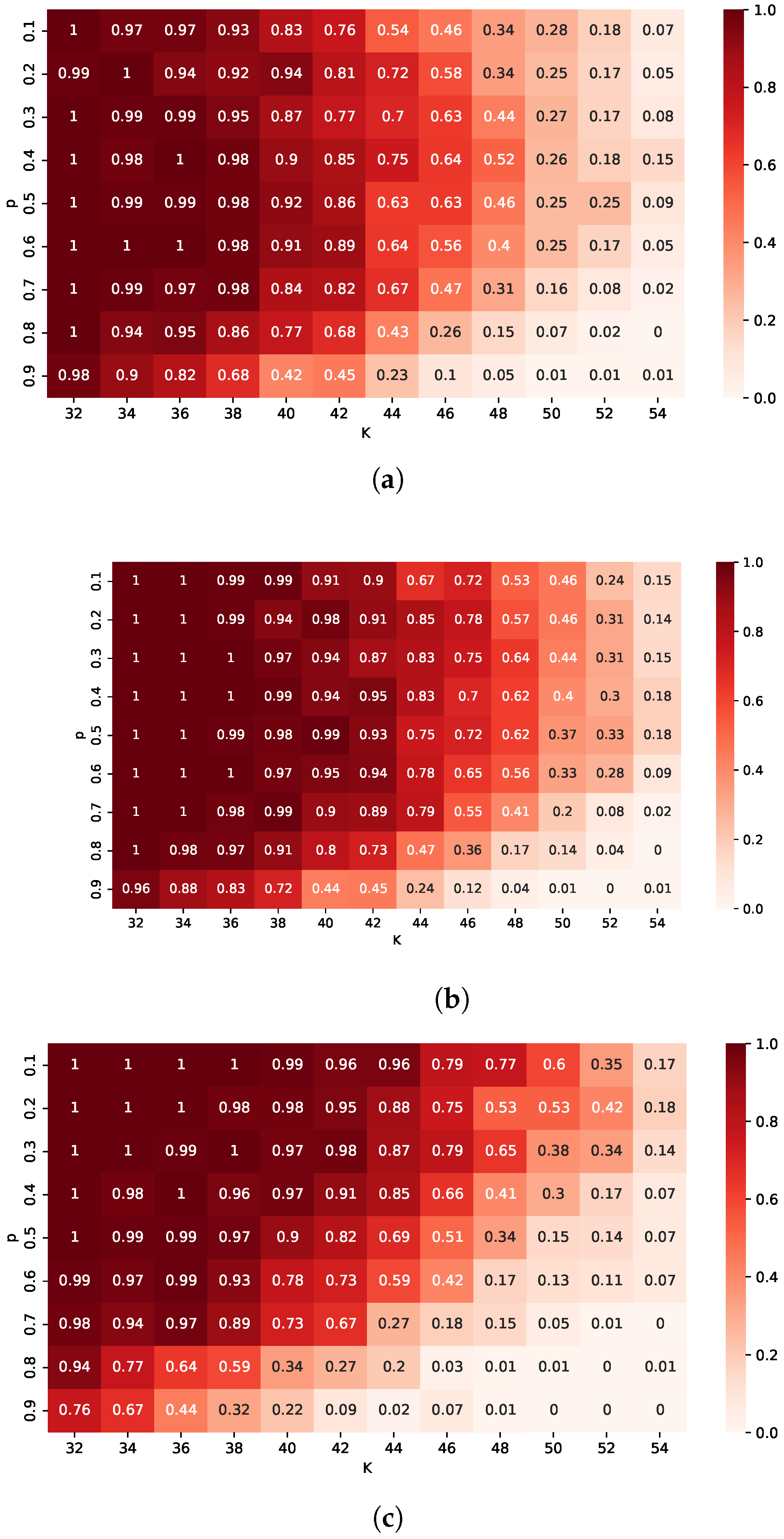
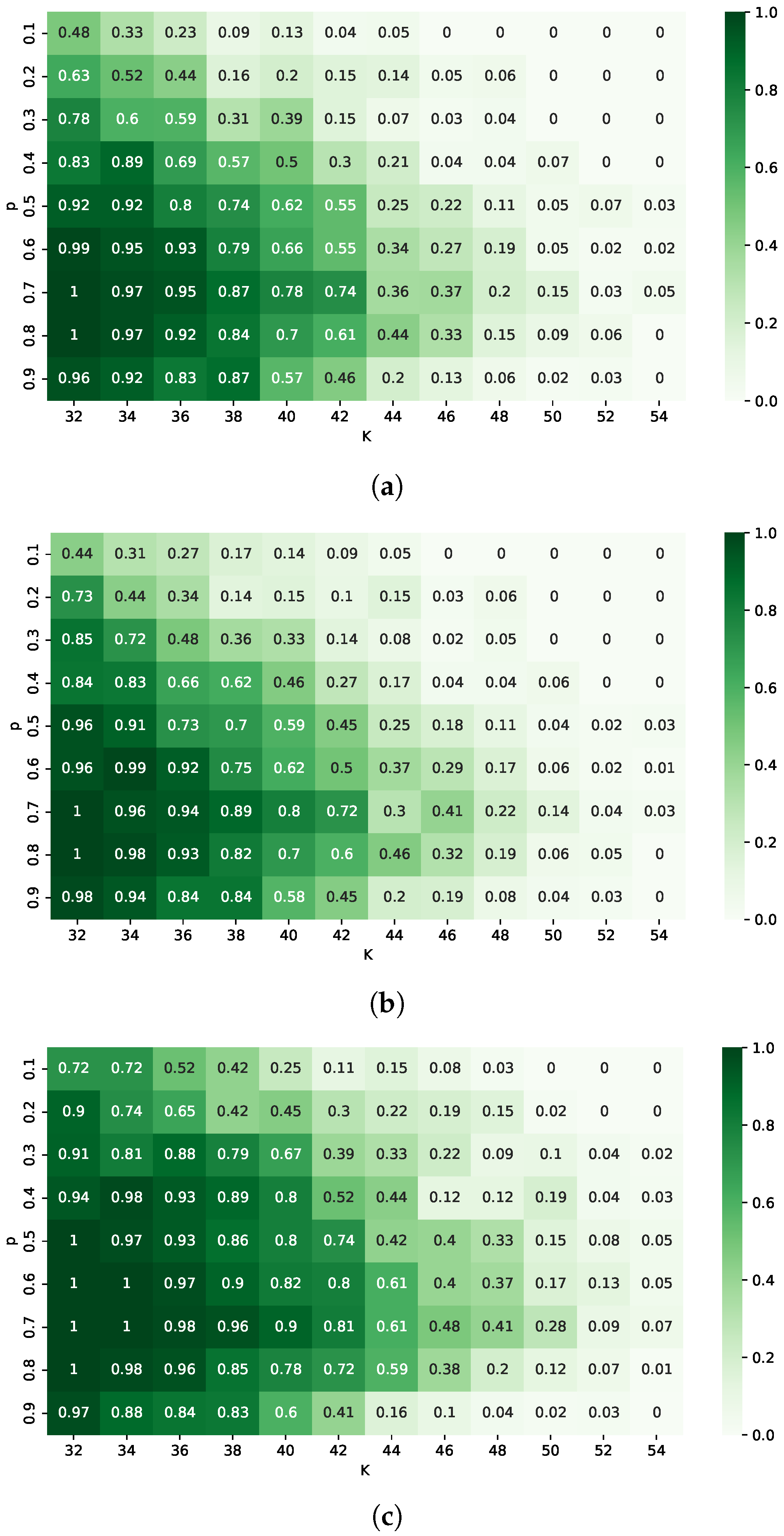
Recovery performance is visualized on the $9\times 12$ grid in Figure 1 and Figure 2. In these diagrams, the x-axis indicates the sparsity level K, while the y-axis represents the parameter p characterizing the quasi-norm. The color at each grid point indicates the recovery success rate averaged over 100 trials. Darker regions denote higher recovery success, while lighter regions indicate failure cases.

The experimental results indicate that the performance of the proposed IR${\ell }_1$ algorithms depends significantly on the signal magnitude and the choice of parameter p. When signal components have small magnitudes ($\sigma =1$), IR${\ell }_1$-2 achieves a notably higher success rate than IR${\ell }_1$-1, especially for smaller values of p. Meanwhile, IR${\ell }_1$-3 performs best at low p, successfully recovering the broadest range of signals. As p approaches one, the performance of IR${\ell }_1$-1 and IR${\ell }_1$-2 converges, whereas that of IR${\ell }_1$-3 deteriorates.

When signal magnitudes are relatively large ($\sigma =10$), the recovery behavior changes. IR${\ell }_1$-3 consistently achieves the highest recovery success, outperforming both IR${\ell }_1$-1 and IR${\ell }_1$-2, except at $p=0.9$, where the latter two perform slightly better. The advantage of $\mathrm{IR}{\ell }_1$-3 increases as p gets smaller. In this scenario, IR${\ell }_1$-1 and IR${\ell }_1$-2 exhibit comparable performance.

To evaluate the robustness of our algorithms to noise, we introduced white noise sampled from a Gaussian distribution with a mean of zero and variance of $\phi$ into the measurement vector b.

Table 1. Average increase in relative error of three algorithms under additive white noise.

		$\mathit{\phi }=0.001$			$\mathit{\phi }=0.005$
	p	IR${\ell }_1$-1	IR${\ell }_1$-2	IR${\ell }_1$-3	IR${\ell }_1$-1	IR${\ell }_1$-2	IR${\ell }_1$-3
$\mathit{\sigma }=\mathbf{1}$	0.1	0.0248%	0.0290%	0.0235%	0.1263%	0.1267%	0.1402%
	0.2	0.0207%	0.0219%	0.0222%	0.1184%	0.1261%	0.1302%
	0.3	0.0237%	0.0251%	0.0265%	0.1234%	0.1216%	0.1268%
	0.4	0.0262%	0.0267%	0.0265%	0.1363%	0.1443%	0.1507%
	0.5	0.0244%	0.0251%	0.0374%	0.1277%	0.1464%	0.1879%
	0.6	0.0298%	0.0332%	0.0410%	0.1337%	0.1266%	0.1964%
	0.7	0.0297%	0.0356%	0.0394%	0.1416%	0.1230%	0.2572%
	0.8	0.0325%	0.0367%	0.0345%	0.2519%	0.1804%	0.9638%
	0.9	0.0416%	0.0381%	0.0926%	0.4835%	0.3896%	1.8213%
	p	IR${\ell }_1$-1	IR${\ell }_1$-2	IR${\ell }_1$-3	IR${\ell }_1$-1	IR${\ell }_1$-2	IR${\ell }_1$-3
$\mathit{\sigma }=\mathbf{10}$	0.1	0.0022%	0.0022%	0.0023%	0.0117%	0.0120%	0.0107%
	0.2	0.0020%	0.0024%	0.0023%	0.0133%	0.0119%	0.0129%
	0.3	0.0024%	0.0025%	0.0023%	0.0120%	0.0118%	0.0122%
	0.4	0.0027%	0.0028%	0.0029%	0.0134%	0.0125%	0.0120%
	0.5	0.0026%	0.0025%	0.0027%	0.0119%	0.0118%	0.0124%
	0.6	0.0024%	0.0024%	0.0023%	0.0125%	0.0123%	0.0130%
	0.7	0.0029%	0.0029%	0.0030%	0.0121%	0.0125%	0.0145%
	0.8	0.0029%	0.0030%	0.0033%	0.0138%	0.0150%	0.0186%
	0.9	0.0027%	0.0028%	0.0034%	0.0199%	0.0204%	0.0307%

presents the average increase in relative recovery error across 100 trials at $K=36$. The results indicate that IR${\ell }_1$-2 exhibits noise robustness comparable to that of IR${\ell }_1$-1, while IR${\ell }_1$-3 is slightly more sensitive to noise, especially when p is close to one or the noise level is higher.

We also recorded the CPU time for each IR${\ell }_1$ algorithm at $K=36$, as shown in Figure 3. Each data point on the chart represents the average absolute CPU time over 100 trials. While computational times generally decrease as p increases, aligning with expectations since the optimization problem becomes closer to a convex formulation, we do not compare computational efficiency across different values of p. Instead, we focus on evaluating the relative performance of different IR${\ell }_1$ algorithms under identical parameter settings.

From an efficiency standpoint, IR${\ell }_1$-3 generally outperforms the other algorithms, with the performance gap widening as p decreases. When the signal component magnitudes are small, IR${\ell }_1$-2 is consistently faster than IR${\ell }_1$-1 but tends to be slightly slower than IR${\ell }_1$-3. When the signal magnitudes are relatively large, IR${\ell }_1$-1 and IR${\ell }_1$-2 exhibit comparable runtimes, while IR${\ell }_1$-3 maintains its efficiency advantage. To further assess efficiency, we also examine the average number of iterations required for convergence, which follows a similar trend to Figure 3. Since each IR${\ell }_1$ method involves similar per-iteration operations with roughly the same expense, the primary determinant of computational cost is the number of iterations. The observed efficiency improvements in the two newly proposed algorithms stem from more accurate approximations of the original ${\ell }_p$ quasi-norm objective, which accelerates convergence.

To summarize, IR${\ell }_1$-2 consistently improves recovery success rate and computational efficiency compared to IR${\ell }_1$ when signal magnitudes are small, while maintaining comparable robustness to noise. On the other hand, IR${\ell }_1$-3 shows the most significant improvements in recovery success rate and efficiency, particularly for large-magnitude signals. However, it is more sensitive to noise in the measurement process, and its performance deteriorates as the sparsity penalty becomes nearly convex (i.e., as p approaches 1).

4. Conclusions

In this paper, we focus on iteratively reweighted ${\ell }_1$-minimization methods for solving the sparse recovery problem based on optimizing the ${\ell }_p$ quasi-norm. Specifically, we propose two novel reweighting strategies, with weights derived from $ϵ$-approximations of ${\parallel x\parallel }_p^p$ that provide enhanced approximation under the same perturbation magnitude. Both reweighting strategies dynamically adjust the weights based on the magnitudes of the current iterate, leading to two distinct IR${\ell }_1$ formulations. Each provides a first-order approximation to a tighter surrogate for the original ${\ell }_p$ quasi-norm objective, thereby facilitating more effective recovery of sparse signals.

The two proposed IR${\ell }_1$ algorithms have been shown to converge to the true sparse solution under appropriate conditions on the sensing matrix. Our experimental results demonstrate that the proposed algorithms show significant improvements in terms of signal recovery success rate and computational efficiency compared to the conventional IR${\ell }_1$ algorithm. The degree of improvement varies depending on the characteristics of the sparse signal. The improvements demonstrated by the proposed IR${\ell }_1$ algorithms become prominent when the sparsity penalty is highly concave (i.e., for smaller p, which favors sparsity). In such cases, the recovered signal is highly likely to match the minimum ${\ell }_0$-norm solution of $Ax=b$ as given in (1).

While our proposed methods improve recovery success and efficiency, they also have certain limitations. One potential drawback is that the performance of our algorithms may be sensitive to noise in the measurement process, which could impact robustness in practical scenarios. Addressing these limitations through adaptive strategies or alternative formulations is an important direction for future research.

Beyond theoretical contributions, our proposed methods have significant practical applications in signal processing, for example, in compressed sensing for efficient signal reconstruction, in medical imaging (MRI and CT) to reduce measurement acquisition while preserving image quality, and in wireless communications for improving channel estimation and reducing interference. By enhancing the accuracy and efficiency of sparse recovery, our algorithms have the potential to contribute to advancements in these critical fields.

This work contributes to the expanding field of sparse recovery by providing more accurate and computationally efficient algorithms for signal reconstruction. Future research may focus on enhancing robustness to noise, and extending these methods to tackle more complex problems in signal processing and machine learning, particularly in applications such as compressed sensing and image recovery.

References

1. Mallat, S. A Wavelet Tour of Signal Processing: The Sparse Way, 3rd ed.; Academic: Cambridge, MA, USA, 2008. [Google Scholar]
2. Qin, Z.; Fan, J.; Liu, Y.; Gao, Y.; Li, G.Y. Sparse representation for wireless communications: A compressive sensing approach. IEEE Signal Process. Mag. 2018, 35, 40–58. [Google Scholar] [CrossRef]
3. Chartrand, R. Exact reconstruction of sparse signals via non-convex minimization. IEEE Signal Process. Lett. 2007, 14, 707–710. [Google Scholar]
4. Chartr, R.; Staneva, V. Restricted isometry properties and non-convex compressive sensing. Inverse Probl. 2008, 24, 035020. [Google Scholar] [CrossRef]
5. Ge, D.; Jiang, X.; Ye, Y. A note on the complexity of Lp minimization. Math. Program. 2011, 129, 285–299. [Google Scholar] [CrossRef]
6. Sun, S.; Pong, T.K. Doubly iteratively reweighted algorithm for constrained compressed sensing models. Comput. Optim. Appl. 2023, 85, 583–619. [Google Scholar] [CrossRef]
7. Yu, P.; Pong, T.K. Iteratively reweighted algorithms with extrapolation. Comput. Optim. Appl. 2019, 73, 353–386. [Google Scholar]
8. Rao, B.D.; Kreutz-Delgado, K. An affine scaling methodology for best basis selection. IEEE Trans. Signal Process. 1999, 47, 187–200. [Google Scholar]
9. Chartrand, R.; Yin, W. Iteratively reweighted algorithms for compressive sensing. In Proceedings of the 2008 IEEE International Conference on Acoustics, Speech and Signal Processing, Las Vegas, NV, USA, 31 March–4 April 2008; pp. 3869–3872. [Google Scholar]
10. Tausiesakul, B. Iteratively reweighted least squares minimization with nonzero index update. In Proceedings of the 2021 Smart Technologies, Communication and Robotics (STCR), Sathyamangalam, India, 9–10 October 2021; pp. 1–6. [Google Scholar]
11. Candès, E.J.; Wakin, M.B.; Boyd, S.P. Enhancing sparsity by reweighted 1 minimization. J. Fourier Anal. Appl. 2008, 14, 877–905. [Google Scholar]
12. Wipf, D.; Nagarajan, S. Iterative reweighted 1 and 2 methods for finding sparse solutions. IEEE J. Sel. Top. Signal Process. 2010, 4, 317–329. [Google Scholar] [CrossRef]
13. Khajehnejad, M.A.; Xu, W.; Avestimehr, A.S.; Hassibi, B. Analyzing weighted 1 minimization for sparse recovery with nonuniform sparse models. IEEE Trans. Signal Process. 2011, 59, 1985–2001. [Google Scholar]
14. Wang, H.; Zhang, F.; Shi, Y.; Hu, Y. Nonconvex and nonsmooth sparse optimization via adaptively iterative reweighted methods. J. Glob. Optim. 2021, 81, 717–748. [Google Scholar]
15. Lu, Z. Iterative reweighted minimization methods for regularized unconstrained nonlinear programming. Math. Program. 2014, 147, 277–307. [Google Scholar]
16. An, Q.; Zhang, N.; Jiang, S. Iterative methods for projection onto the p quasi-norm ball. Optim. Methods Softw. 2024, 1–22. [Google Scholar] [CrossRef]
17. Gorodnitsky, I.F.; Rao, B.D. Sparse signal reconstruction from limited data using FOCUSS: A re-weighted minimum norm algorithm. IEEE Trans. Signal Process. 1997, 45, 600–616. [Google Scholar] [CrossRef]
Figure 1. Success rates of exact recovery for the algorithms (a) IR 1 -1, (b) IR 1 -2, and (c) IR 1 -3, with σ = 1 .
Mathematics 13 01219 g001
Figure 2. Success rates of exact recovery for the algorithms (a) IR 1 -1, (b) IR 1 -2, and (c) IR 1 -3, with σ = 10 .
Mathematics 13 01219 g002
Figure 3. Average computational time of three algorithms with (a) σ = 1 and (b) σ = 10 .
Mathematics 13 01219 g003