A Hubness Information-Based k-Nearest Neighbor Approach for Multi-Label Learning

Abstract

Multi-label classification (MLC) plays a crucial role in various real-world scenarios. Prediction with nearest neighbors has achieved competitive performance in MLC. Hubness, a phenomenon in which a few points appear in the k-nearest neighbor (kNN) lists of many points in high-dimensional spaces, may significantly impact machine learning applications and has recently attracted extensive attention. However, it has not been adequately addressed in developing MLC algorithms. To address this issue, we propose a hubness-aware kNN-based MLC algorithm in this paper, named multi-label hubness information-based k-nearest neighbor (MLHiKNN). Specifically, we introduce a fuzzy measure of label relevance and employ a weighted kNN scheme. The hubness information is used to compute each training example’s membership in relevance and irrelevance to each label and calculate weights for the nearest neighbors of a query point. Then, MLHiKNN exploits high-order label correlations by training a logistic regression model for each label using the kNN voting results with respect to all possible labels. Experimental results on 28 benchmark datasets demonstrate that MLHiKNN is competitive among the compared methods, including nine well-established MLC algorithms and three commonly used hubness reduction techniques, in dealing with MLC problems.

1. Introduction

Multi-label learning solves one of the main categories of machine learning classification tasks, where each instance could belong to multiple labels simultaneously. For example, a news document could be labeled by multiple topics simultaneously, such as environment, health, and technology. An image scene could contain various concepts, such as buildings, cars, and pavement. Multi-label classification (MLC) problems widely exist in both daily life and specialized fields, such as social media tagging [1], product categorization [2], remote sensing image classification [3], and legal text mining [4]. This leads to a significant demand for efficient and accurate MLC algorithms.

A key difference in designing MLC algorithms compared to single-label classification (SLC) algorithms is that MLC algorithms can leverage label correlations, which are derived from the co-occurrence of labels in multi-label datasets (MLDs), to improve their performance. Many MLC algorithms across various domains have been proposed. Existing methods can be categorized into first-order, second-order, and high-order approaches, which consider no correlation, pairwise correlations, and correlations among multiple labels. Higher-order approaches can explore more complex relationships, which is helpful in improving the classifier performance. The k-nearest neighbor (kNN) search technique is employed in some popular MLC algorithms, such as first-order methods, BRkNN [5] and MLKNN [6], and high-order methods, DMLkNN [7] and IBLR [8]. These kNN-based approaches achieve competitive performance among existing MLC algorithms [9,10] and constitute one of the major branches in multi-label learning.

Recently, an issue related to the kNN search, hubness in high-dimensional data, has drawn extensive attention in various machine learning areas. It refers to the phenomenon where a small number of points appear in the k-neighborhoods of a large number of examples. Specifically, let the k-occurrence of point x, $O_k\left(x\right)$, denote the number of times x appears among the k nearest neighbors of all other points in a dataset. The average k-occurrence of all points is k. Some popular examples may have k-occurrences several times larger than k, and some may be included in the k-neighborhoods of very few or no other points. These two types of points are called hubs and antihubs, respectively. Hubness is an inherent property of data distributions in high-dimensional space under widely used assumptions and is not caused by other effects such as finite sample size [11]. Existing studies have shown that the hubness problem can have a significant impact on the performance of machine learning algorithms involving kNN search in high dimensions [11,12]. Take the classification task, for example. Let the term bad k-occurrence represent that a point lies in the k-neighborhood of another point, but the two points’ labels do not match. Empirical results indicate that hubs are more prone to picking up bad k-occurrence in high dimensions than other points. Similarly, hubs are more likely to appear in the kNN lists of query points and belong to different classes from those of the query points. Existing studies show that dimensionality reduction may not have a significant effect on reducing hubness until intrinsic dimensionality is reached [11]. However, there may be a loss of information if the dimensionality is further reduced. Some techniques have been proposed to mitigate the negative effects of hubness in machine learning and have achieved significant improvements. On the other hand, existing hubness-aware approaches for classification tasks mainly focus on single-label cases.

To illustrate the hubness phenomenon in MLDs, we show the distributions of $O_k\left(x\right)$ and the k-occurrence skewness $S_k$, which is typically used to measure the degree of hubness, of some benchmark MLDs with different dimensionalities in Figure 1. $S_k$ is the standardized third central moment of the k-occurrence distribution.

$$\begin{array}{c}\hfill S_k={\displaystyle \frac{E{(O_k-{\mu }_{O_k})}^3}{{\sigma }_{O_k}^3}},\end{array}$$

(1)

where ${\mu }_{O_k}$ and ${\sigma }_{O_k}$ are the mean and standard deviation of $O_k$, respectively. $S_k$ characterizes the asymmetry of $O_k$. It signifies skewness to the right (left) for $S_k$ with a positive (negative) value and no skewness for $S_k=0$. Higher skewness to the right indicates a higher degree of hubness. As shown in Figure 1, in the six datasets with relatively higher dimensions, the highest probability density occurs at $O_k=0$, corresponding to antihubs. Meanwhile, a few points have values of $O_k$ several tens of times greater than k, corresponding to hubs. In Figure 1, five multi-label datasets have the values of $S_k$ varying from 9.92 to 23.24. Note that among the 50 different machine learning datasets employed in an empirical comparison study of hubness reduction methods [12], 47 datasets have values of $S_k$ varying from −0.12 to 5.58. The other three datasets have $S_k$ values of 9.35, 10.71, and 15.52, respectively. By comparison, these MLDs exhibit high degrees of hubness. For that, in this paper, we propose a hubness-aware kNN-based MLC algorithm named MLHiKNN, i.e., multi-label hubness information-based k-nearest neighbor. To address the hubness issue, MLHiKNN introduces a fuzzy measure of label relevance for training examples and uses hubness weighting for different neighbors. Specifically, the degree of a training example’s support for a label is determined by its relevance to the label, its history k-occurrence, and the labels of its reverse nearest neighbors. Further, MLHiKNN trains a logistic regression model with the kNN voting results with respect to all possible labels. Thus, it is a high-order method with respect to label correlation. As far as we know, it is the first approach to address the hubness issue in MLC. We conducted experiments on twenty-eight benchmark MLDs from different domains to compare MLHiKNN with nine well-established MLC algorithms and three commonly used hubness reduction techniques. Experimental results show that MLHiKNN achieves the best performance in a considerable number of scenarios, indicating that it is highly competitive among the compared methods. The remainder of this paper is organized as follows: Section 2 reviews some MLC algorithms and hubness-aware techniques. Section 3 introduces the framework and details of the proposed method. Section 4 reports and discusses the results of experiments for method comparison, ablation analysis, and parameter analysis. Section 5 concludes this work.

Figure 1. Empirical distributions of $O^k$ and the k-occurrence skewness (for the datasets Slashdot, bibtex, and eurlex-dc-leaves, $O^k$ and $S_k$ are computed based on the dimensionality-reduced feature space), where $k=10$, of nine MLDs with different dimensionalities.

2. Related Work

This section reviews the existing MLC algorithms, followed by the works addressing the hubness phenomenon in high-dimensional spaces.

2.1. Multi-Label Classification Algorithms

Let a multi-label dataset be denoted by $D=\left\{({\mathbf{x}}_i,{\mathbf{y}}_{x_i})\right|1\le i\le n\}$, where the feature vector ${\mathbf{x}}_i={(x_{i1},x_{i2},\dots ,x_{id})}^T$, and the label indicator vector ${\mathbf{y}}_{x_i}={(y_{x_i}^1,y_{x_i}^2,\dots ,y_{x_i}^q)}^T$. n is the number of examples in D, q is the number of possible labels, and d is the number of features. $y_{x_i}^j=1$ if example $x_i$ belongs to the j-th label and $y_{x_i}^j=0$ otherwise. Multi-label learning is learning to map from the feature space to the label space with a dataset like D, and then predict the label indicator vector for each query example with its features. Existing MLC algorithms can be divided into problem transformation methods and algorithm adaptation methods based on the strategy for making an MLC problem solvable with SLC algorithms. Further, many efforts have been made to exploit correlations among labels to improve the generalization ability of an MLC algorithm. Existing MLC algorithms can also be roughly categorized into first-order, second-order, and high-order approaches according to the order of correlations being considered [13].

Problem transformation methods fit data to the algorithm by transforming a multi-label dataset into multiple single-label datasets (SLDs). Then, a sub-problem is solved with SLC algorithms for each single-label dataset. BR [14] transforms the original MLC problem into q binary classification sub-problems, where each sub-problem corresponds to one possible label and takes the original features as inputs. BR belongs to first-order approaches, which do not consider label correlations. Second-order approaches consider the correlations between each pair of labels. These approaches usually generate a sub-problem for each pair of possible labels, such as CLR [15] and RPC [16], which generate $q(q-1)/2$ sub-problems in total. High-order approaches consider the correlations among multiple labels. For example, CC [17] constructs a chain of binary classifiers, where each classifier corresponds to one label. Different from BR, each binary classifier in CC considers the labels corresponding to the previous binary classifiers as additional features for prediction. However, a drawback of CC is that the pattern of correlations depends on the order of binary classifiers, which is predetermined. ECC [17], the ensemble version of CC, deals with this problem by building a set of CC models, where the order of binary classifiers is randomly generated for each model. Another representative high-order approach, LP [14], transforms the original MLC problem into a multi-class classification problem, where each class corresponds to a distinct label set that appeared in the dataset. LP has two major limitations. One is that LP cannot predict unseen label sets based on the training set. The other is that LP is inefficient since the number of classes in the transformed problem may be very large for a dataset with a large q. RAkEL [18], the ensemble version of LP, tackles the two drawbacks by employing many LP models, where each model only deals with several labels. These LP models overlap in labels and cover all possible labels together. On the other hand, RAkELd [18] splits all the possible labels to these LP models without overlap.

Algorithm adaptation methods fit the algorithm to the data by modifying the components of an SLC algorithm to deal with MLDs directly. For example, ML-DT [19] modifies the C4.5 approach by allowing multiple labels in the leaves to deal with multi-label data. Rank-SVM [20] adapts the maximum-margin strategy to learn from multi-label data. ML-RBF [21] adapts the Radial Basis Function for multi-label learning. kNN-based methods also constitute a major branch of this category of approaches. BRkNN [5] is conceptually equivalent to using BR as the problem transformation method and the KNN algorithm as the base classifier. In practice, BRkNN only needs to search for the k nearest neighbors (kNNs) of each example for a single time. BRkNNa [5] extends BRkNN by avoiding the empty output when predicting a label set. Unlike BRkNN, which compares the positive and negative votes from the kNNs to make predictions, MLKNN [6] follows a maximum a posteriori (MAP) principle based on the counts of positive neighbors to predict the relevance to each label. Thus, the information of training examples far from the query sample also contributes to the prediction in MLKNN. Meanwhile, MLKNN is less affected by class imbalance than BRkNN. ML-k’sNN [22] extends MLKNN by searching and applying the best parameter k, which is the number of nearest neighbors to take into account, for the prediction of each label. The above kNN-based MLC algorithms are all first-order approaches. The high-order approach DMLkNN [7] extends MLKNN by taking into consideration the occurrences of all other labels in the MAP model besides the label to be predicted. IBLR [8] exploits high-order correlations by augmenting the original features with the labels of the kNNs of an instance when training a logistic regression model for each label.

Recently, many works have attempted to address some more specific challenges in multi-label learning [23], such as class imbalance [24], the different types of supervision like MLC with missing labels [25,26] and partial multi-label learning [27,28], the extremely large number of labels [29,30], and online multi-label learning [31,32]. Nevertheless, as far as we know, the hubness problem has not been addressed in MLC. The following subsection will review some studies about the hubness phenomenon and existing techniques focusing on learning with hubs in SLC.

2.2. Methods Addressing the Hubness Problem

Hubness is one aspect of the curse of dimensionality when performing a search for nearest neighbors. The hubness problem was first noted in audio-based music recommendation [33]. Specifically, a small number of hub songs are recommended conspicuously frequently in nearest neighbor-based playlists. Radovanović et al. studied the causes and implications of hubness extensively from both theoretical and empirical perspectives [11]. The hubness phenomenon is related to data concentration, another aspect of the dimensionality curse. The phenomenon of data concentration is usually expressed as the ratio between some measure of spread and magnitude, such as the ratio between the standard deviation and the mean of the distances to an arbitrary reference point of all points. If this ratio converges to zero as the dimensionality approaches infinity, it is said that the distances concentrate, indicating that all points are almost at the same distance from the reference point. Theoretical analysis in existing works indicates that points in high dimensions are approximately lying on a hypersphere centered at the data mean. Radovanović et al. proposed the argument that the points closer to the data mean are more likely to become hubs, and points further away from the data mean are more likely to be antihubs in high dimensions [11]. The nearest-neighbor search is an essential component in many commonly used algorithms for a wide range of machine learning applications, such as classification, regression, clustering, and outlier detection. For these algorithms, the hubness problem can have a significant impact on their performance in high dimensions. There have been some studies addressing this issue across various application domains. We roughly divide existing techniques into distance transformation and algorithm adaptation methods.

Distance transformation methods can be incorporated into the nearest-neighbor search process of various algorithms. These methods reduce hubness by modifying the neighbor graph through alternative dissimilarity measures and distance metrics, re-scaling, centering, and other techniques. Alternative dissimilarity measure techniques directly operate on the position vectors of each point for pairwise dissimilarities. Then, the dissimilarities are used instead of the original distances in the search for nearest neighbors to reduce hubness. These hubness-aware measures typically consider the information of other points as an addition when computing the dissimilarity between each pair of points. DSL [34] flattens the density gradient to reduce spatial centrality in Euclidean spaces. For two examples, $x_1$ and $x_2$, DSL calculates their dissimilarity by removing the sample-wise centrality from their distance,

$$\begin{array}{c}\hfill \mathrm{DSL}(x_1,x_2)=\parallel x_1-x_2{\parallel }_2^2-\parallel x_1-c_k\left(x_1\right){\parallel }_2^2-{\parallel x_2-c_k\left(x_2\right)\parallel }_2^2.\end{array}$$

(2)

Let $D_k\left(x\right)$ be a set consisting of the kNNs of x. $c_k\left(x\right)={\displaystyle \frac{1}{k}}{\sum }_{x^{\prime }\in D_k\left(x\right)}{x}^{\prime }$ is a local centroid with respect to x. Parameter k is the number of nearest neighbors considered to compute centroids. $m_p$-dissimilarity [35] is calculated based on probability mass and follows the principle that two points in a sparse region are more similar than two points in a dense region. $simhu{b}_s^{\mathrm{IN}}$ [36] is based on the observation that a rarely shared neighbor (antihub) is more informative than a commonly shared neighbor (hub) in similarity calculation. Unlike the above three measures, which rely only on feature vectors, the following two measures incorporate class information for dissimilarity computation and are specifically for classification tasks. MADD [37] is based on the mean absolute difference between inter-point pairwise distances. $simhu{b}_s^{\mathrm{PUR}}$ [36] prefers the points whose reverse neighbors are almost exclusively from the same class compared to those with reverse neighbors from various classes when computing similarities. The incorporation of class information in the two techniques does not generally reduce hubness like other distance transformation methods but can be regarded as trying to preserve similarities with the hubs, which can provide helpful information for classification, and to reduce similarities with the hubs that offer no benefit for classification. Note that the two techniques are not applicable to multi-label scenarios. Alternative distance metric techniques do not utilize the information of other points to compute the distance between each pair of points but use hubness-aware metrics to reduce hubness. Aggarwal et al. showed that fractional norms are less prone to distance concentration than the Euclidean norm [38]. To be specific, despite all ${\ell }_p$ norms exhibiting concentration, the degree of concentration is influenced by both the distribution of data and the value of p. Based on this observation, Flexer et al. define antihub occurrence as the percentage of antihubs in the dataset and hub occurrence as the percentage of hubs in all nearest-neighbor slots. Then, the authors reduce hubness by choosing the ${\ell }_p$ norm, by which the corresponding antihub occurrence or hub occurrence is minimal [39].

Re-scaling techniques compute the pairwise distances using a well-established metric, such as the Euclidean distance, first. Then, they scale the distance between each pair of points based on other pairwise distances, considering a local or global perspective. Local scaling (LS) and mutual proximity (MP) [40,41] are two representative re-scaling techniques. They reduce hubness by repairing asymmetric neighbor relations by computing pairwise secondary distances. For two examples $x_1$ and $x_2$, LS scales their original distance $d_{x_1,x_2}$ using the local distance information of the two examples,

$$\begin{array}{c}\hfill \mathrm{LS}(x_1,x_2)=1-exp(-{\displaystyle \frac{d_{x_1,x_2}^2}{d_k\left(x_1\right)d_k\left(x_2\right)}}),\end{array}$$

(3)

where $d_k\left(x\right)$ is the distance between x and its k-th nearest neighbor. Unlike LS, which uses local distance as the scaling parameter, MP considers all pairwise distances in the dataset. MP calculates the proximity between $x_1$ and $x_2$ by the number of instances whose distances to $x_1$ and $x_2$ are both greater than $d_{x_1,x_2}$,

$$\begin{array}{c}\hfill \mathrm{MP}(x_1,x_2)={\displaystyle \frac{|\left\{j\right|d_{x_1,j}>d_{x_1,x_2}\}\cap \left\{j\right|d_{x_2,j}>d_{x_2,x_1}\}|}{n-2}},\end{array}$$

(4)

where n is the number of examples in the dataset. Centering techniques were also shown to be effective in reducing hubness. CENT [42] shifts the origin space to the global data centroid and uses inner product similarities. LCENT [43] further considers local centroids for the datasets where the sample size is large and the dimension of vectors is not necessarily very high. Distance transformation hubness reduction techniques have been verified to be effective in improving algorithm performance across datasets from different domains and have been employed in various applications, such as knowledge graph embedding [44], single-cell omics profiling [45], and Sentence-BERT embedding [46].

Algorithm adaptation methods modify existing algorithms involving nearest-neighbor search to deal with the hubness problem. The kNN classifier has naturally become one of the most noted algorithms, with hubness-aware modifications being implemented in existing studies. hw-kNN [47] reduces the voting weights of bad hubs, which refer to the hub examples whose labels do not match those of their reverse nearest neighbors. Concretely, the weight assigned to a point x is based on the count of bad occurrences for x, where a bad occurrence is defined as a reverse nearest neighbor belonging to a different class from that of x. NHBNN [48] performs a Naive-Bayesian inference for each query point according to the kNNs. For each neighbor of a query point, a probability estimation is conducted based on the labels of its historical reverse nearest neighbors in the training set. h-FNN [49] modifies the class preference provided to query points of each training example by introducing fuzzy measures. The fuzzy membership of a training point x in each class is related to the percentage of samples in this class among all reverse nearest neighbors of x. Meanwhile, for points rarely appearing in the kNN lists of other points, h-FNN offers four alternative approaches to estimate their fuzziness from a global or local perspective. Distance weighting can also be incorporated into the h-FNN framework. HIKNN [50] utilizes the historical occurrence information to adjust both the weights and class preferences of training examples in kNN voting. Specifically, antihubs are more informative than hubs. The class preference of a training point depends on both its label and the labels of its reverse nearest neighbors.

There have also been some studies that focus on dealing with hubness in other machine learning tasks, such as regression, clustering, and outlier detection. For the case of regression, EWCkNN [51], on the one hand, performs error-based weighted k-nearest-neighbor regression, where the weight of a point x is inversely related to the normalized average absolute difference between the label of x and the labels of x’s k reverse nearest neighbors. On the other hand, it uses the corrected labels for prediction, where the corrected label of a training point x is defined as the average of the labels of x’s k reverse nearest neighbors. For the case of clustering, the K-hubs [52] approach uses hubs in the same way that centroids are typically used and converges to final clusters very quickly. GHPC [52] implements a squared hubness–proportional stochastic scheme and uses the simulated annealing approach for optimization. For the case of outlier detection, the ${\mathrm{AntiHub}}^2$ [53] approach computes an outlier score for each point x by considering the occurrence numbers of both x and x’s neighbors in the kNN lists of other points. PEHS [54] constructs a digraph based on the neighborhood relations of points and performs a tailored Markov random walk process on the digraph to derive a hubness score for each point. Then, it brings together the hubness score and the potential energy of a point, which is derived from the concept of potential of particles in physics, for an importance degree. Points with small degrees of importance are considered outliers.

Besides the works mentioned above, the hubness issue has also been addressed in some specific applications. For example, zero-shot learning involves nearest-neighbor searches in a learned high-dimensional embedding space as the last step and thus suffers from the hubness issue. It is also shown that ridge regression tends to promote hubness in regression-based zero-shot learning [55]. Different techniques have been pursued to deal with the hubness issue in zero-shot learning, such as considering the global distribution of test data in a transductive way [56], using the visual feature space of a CNN subnet as the embedding space [57], modifying the objective function to maximize the scatter between different classes besides the attribute regression accuracy [58], and learning a latent space preserving the semantic relationship and discriminating information [59]. Besides the works in zero-shot learning, HLM [60] extends the Bipartite Local Model (BLM), a leading method for drug–target interaction prediction, by incorporating the ECkNN approach, a hubness-aware regression technique that corrects the label of a training point by the labels of its reverse nearest neighbors. Wang et al. proposed a hybrid similarity measurement that combines rating-based and structural similarity measurements to deal with the hubness problem in memory-based collaborative filtering, a recommendation system method for user’s rating or preference prediction [61]. Tian et al. proposed a novel retrieval measuring metric that includes the hubness degree as a penalty factor to alleviate the hubness issue in similarity-based translation memory retrieval for ontology translation [62]. The proposed method, MLHiKNN, can be categorized into the algorithm adaptation category for dealing with the hubness issue. The details will be introduced in the following section.

3. The Proposed Method: MLHiKNN

The major components in the model of MLHiKNN include the label relevance score (Section 3.1) used to leverage the hubness information of nearest neighbors and a label predictor (Section 3.4), where the label relevance scores are considered as the features of a query instance. The elements used for computing label relevance scores are introduced in Section 3.2 and Section 3.3. The complete steps of MLHiKNN are introduced in Section 3.4.

3.1. Label Relevance Score for Query Points

For each query instance t whose label set is to be estimated, we first introduce its positive and negative voting scores with respect to label l, $v_1^l\left(t\right)$ and $v_0^l\left(t\right)$. Let $D_k\left(t\right)$ be the set consisting of the kNNs of t. $v_1^l\left(t\right)$ and $v_0^l\left(t\right)$ are the results of weighted voting by considering the label and hubness information of all instances in $D_k\left(t\right)$ as follows:

$$\begin{array}{c}\hfill v_b^l\left(t\right)=\sum _{x\in D_k\left(t\right)}{w}_d(t,x)·w_h(t,x)·u_b^l\left(x\right),b\in \{0,1\},\end{array}$$

(5)

where $u_b^l\left(x\right)$ is the fuzzy membership of x with respect to label l (Section 3.2). $w_d(t,x)$ and $w_h(t,x)$ (Section 3.3) are two factors to adjust the voting weights among the kNNs of t. Then, the label relevance score of t with respect to label l is obtained as follows:

$$\begin{array}{c}\hfill r^l\left(t\right)={\displaystyle \frac{v_1^l\left(t\right)}{v_0^l\left(t\right)+v_1^l\left(t\right)}}.\end{array}$$

(6)

Instance t is more likely to be relevant to label l if it has a larger $r^l\left(t\right)$. The computation of the label relevance score involves hubness information in both the fuzzy membership $u_b^l\left(x\right)$ and the weight factor $w_h$. The details are introduced in the following subsections.

3.2. Fuzzy Measure of Label Relevance for Training Points

For a point x, its degree of hubness is measured by its k-occurrence $O_k\left(x\right)$, which is the number of times x appears among the kNNs of all other points in the dataset. This is also known as the size of the k reverse neighborhood of x. The label hubness of x with respect to label l is measured by its label k-occurrence, $O_k^l\left(x\right)$, which refers to the number of instances relevant to label l in the k reverse neighborhood of x. In this work, we append each instance to its own k-neighborhood (resulting in $k+1$ points in the k-neighborhood) when computing k-occurrence and label k-occurrence in case k-occurrence is zero for some points, leading to tedious formulas in the proposed approach. The procedures of counting k-occurrence and label k-occurrence are shown in Algorithm 1.

Algorithm 1 k-occurrence counting.

Input:

D: training set;

k: number of nearest neighbors to take into account.

Output:

$O_k\left(x\right),O_k^l\left(x\right)$: the k-occurrence and label k-occurrence with respect to each possible label l of each instance x in D.   1: $q\leftarrow$ number of possible labels in D   2: find the k-neighborhood $D_k\left(x\right)$ for each instance x in D   3: for each instance x in D do   4:      $O_k\left(x\right)\leftarrow 0$   5:      for $l\leftarrow 1 \mathbf{to} q$ do   6:          $O_k^l\left(x\right)\leftarrow 0$   7:      end for   8:      for each instance $x^{\prime }$ in D do   9:          if $x\in D_k\left(x^{\prime }\right)$ then 10:             $O_k\left(x\right)\leftarrow O_k\left(x\right)+1$ 11:             for $l\leftarrow 1 \mathbf{to} q$ do 12:                 if $y_{x^{\prime }}^l=1$ then 13:                     $O_k^l\left(x\right)\leftarrow O_k^l\left(x\right)+1$ 14:                 end if 15:             end for 16:          end if 17:      end for 18: end for 19: return $\{O_k\left(x\right),O_k^l\left(x\right)|x\in D,1\le l\le q\}$

Given the condition that x is in the k-neighborhood of an unlabeled instance t, the probability that t is relevant to label l can be obtained based on $O_k\left(x\right)$ and $O_k^l\left(x\right)$ as follows:

$$\begin{array}{cc}\hfill & P(y_t^l=1|x\in D_k\left(t\right))={\displaystyle \frac{O_k^l\left(x\right)+s}{O_k\left(x\right)+s\times 2}},\hfill \end{array}$$

(7)

where s is a smoothing parameter. In this work, s is set to be 1 (Laplace smoothing). Let $p_1^l\left(x\right)$ denote the above conditional probability and $p_0^l\left(x\right)$ denote such a conditional probability that t is irrelevant to label l.

$$\begin{array}{c}\hfill p_0^l\left(x\right)=P(y_t^l=0|x\in D_k\left(t\right))=1-p_1^l\left(x\right).\end{array}$$

(8)

From the perspective of probability estimation, t is more likely to be relevant to label l if x has a greater $p_1^l\left(x\right)$. Estimation with $p_1^l\left(x\right)$ is appropriate for x with a large $O_k\left(x\right)$ according to the law of large numbers. For x with a small $O_k\left(x\right)$, an appropriate alternative, following the principle in the KNN classifier, is to assume that t is more likely to have label l if x has label l. The conclusions drawn from the two clues might be inconsistent for hubs that are more prone to picking up bad k-occurrence in high dimensions. Accordingly, we introduce the fuzzy measure of label relevance to consider both the label and hubness information of an instance in the training set. Let $u_1^l\left(x\right)$ and $u_0^l\left(x\right)$ denote the degrees of membership of instance x in terms of relevance and irrelevance to label l, respectively.

$$\begin{array}{cc}\hfill & u_1^l\left(x\right)=g\left(x\right)·y_x^l+(1-g\left(x\right))·p_1^l\left(x\right),\hfill \end{array}$$

(9)

$$\begin{array}{cc}\hfill & u_0^l\left(x\right)=g\left(x\right)·(1-y_x^l)+(1-g\left(x\right))·p_0^l\left(x\right),\hfill \end{array}$$

(10)

where $g\left(x\right)$ is a factor that weighs the label and hubness information of a labeled instance x.

For an appropriate function $g\left(x\right)$, the following conditions for the generation of fuzzy sets need to be satisfied first. For each label l,

$$\begin{array}{cc}\hfill & \sum _{b\in \{0,1\}}{u}_b^l\left(x\right)=1,\hfill \end{array}$$

(11)

$$\begin{array}{cc}\hfill & 0<\sum _{x\in D}{u}_b^l\left(x\right)<\left|D\right|,\hfill \end{array}$$

(12)

$$\begin{array}{cc}\hfill & u_b^l\left(x\right)\in [0,1].\hfill \end{array}$$

(13)

Equation (11) always holds according to the function of $u_b^l\left(x\right)$ in Equations (9) and (10). Equation (12) is to avoid the situation where all points certainly belong to the same fuzzy set. Equation (13) is to ensure the reasonable range of membership.

Second, we set $g\left(x\right)$ to be in $[0,1]$ as a weight factor. It reflects the intuition that the predictive importance of x’s own labels should decrease as x appears more frequently in the k-neighborhoods of other training instances. When a training instance x is rarely selected as a neighbor by other training instances (i.e., $O_k\left(x\right)$ is small), its own labels are essential for making predictions for a query point. In the extreme case where x does not appear in the k-neighborhood of any other training point, only its own labels are available for label prediction, and hence, we define $g\left(x\right)=1$.

$$\begin{array}{c}\hfill g\left(x\right)=1,\mathrm{if}{O}_k\left(x\right)=1.\end{array}$$

(14)

As $O_k\left(x\right)$ increases, it becomes possible to estimate the query label based on the labels of other instances for which x is in the k-neighborhoods. Thus, the weight assigned to x’s own label set should gradually decrease. The hubness information contributes more to the fuzzy membership $u_b^l\left(x\right)$. We define a threshold $\lambda k$, where $\lambda$ is a preset parameter, such that when $O_k\left(x\right)\ge \lambda k$, the contribution of x’s own label set is reduced to zero, i.e., $g\left(x\right)=0$. At this point, we consider that the hubness information provides significantly more informative value than the labels of x. The threshold is proportional to k since a larger k usually leads to a larger $O_k$ for each instance. The parameter $\lambda$ determines how the threshold changes with respect to k. The use of $\lambda k$ is also motivated by the observation in previous research that an example is typically identified as a hub if its k-occurrence is larger than $2k$. In such cases, a point’s frequent appearance in k-neighborhoods is often caused by the hubness phenomenon rather than label similarity, making its label less reliable for prediction. Empirically, we found that setting $\lambda =2$ yields good average performance, in line with the threshold commonly adopted in the literature for hub definition. A detailed parameter analysis is provided in Section 4.5.

$$\begin{array}{c}\hfill g\left(x\right)=0,\mathrm{if}{O}_k\left(x\right)\ge \lambda k.\end{array}$$

(15)

For x with $O_k\left(x\right)$ between 1 and $\lambda k$, $g\left(x\right)$ is in $(0,1)$.

$$\begin{array}{c}\hfill 0<g\left(x\right)<1,\mathrm{if}1<O_k\left(x\right)<\lambda k.\end{array}$$

(16)

Third, for x with $O_k\left(x\right)$ in the range of $(1,\lambda k)$, the derivative of $g\left(x\right)$ with respect to $O_k\left(x\right)$ is expected to be less than 0,

$$\begin{array}{c}\hfill {\displaystyle \frac{\mathrm{d}g\left(x\right)}{\mathrm{d}{O}_k\left(x\right)}}<0,\mathrm{if}1<O_k\left(x\right)<\lambda k,\end{array}$$

(17)

so that as $O_k\left(x\right)$ increases, the weight of $p_b^l\left(x\right),b\in \{0,1\}$, increases, and the weight of $y_x^l$ decreases. Meanwhile, the second-order derivative of $g\left(x\right)$ with respect to $O_k\left(x\right)$ is expected to be larger than 0 for x with $O_k\left(x\right)$ in $(1,\lambda k)$,

$$\begin{array}{c}\hfill {\displaystyle \frac{{\mathrm{d}}^{2}g\left(x\right)}{\mathrm{d}{O}_k{\left(x\right)}^2}}>0,\mathrm{if}1<O_k\left(x\right)<\lambda k.\end{array}$$

(18)

For example, assume four points $x_1$, $x_2$, $x_3$, and $x_4$ with k-occurrences of 1, 10, 51, and 60. The difference in k-occurrence between $x_1$ and $x_2$ is equal to that between $x_3$ and $x_4$, $O_k\left(x_4\right)-O_k\left(x_3\right)=O_k\left(x_2\right)-O_k\left(x_1\right)$. On the other hand, the difference in importance when calculating the membership of label relevance between $p_b^l\left(x_1\right)$ and $p_b^l\left(x_2\right)$ is expected to be greater than that between $p_b^l\left(x_3\right)$ and $p_b^l\left(x_4\right)$, due to the rate of change in k-occurrence being larger from $x_1$ to $x_2$ than from $x_3$ to $x_4$. This results in a corresponding difference in their weights. Specifically, $(1-g\left(x_2\right))-(1-g\left(x_1\right))>(1-g\left(x_4\right))-(1-g\left(x_3\right))$, which simplifies to $g\left(x_4\right)-g\left(x_3\right)>g\left(x_2\right)-g\left(x_1\right)$. Based on the above considerations in Equations (11)–(18), we define the function of $g\left(x\right)$ as follows:

$$\begin{array}{cc}\hfill g\left(x\right)& ={\displaystyle \frac{{log}_{\gamma }\lambda k-{log}_{\gamma }min(O_k\left(x\right),\lambda k)}{{log}_{\gamma }\lambda k}}\hfill \\ \hfill & =1-{log}_{\lambda k}min(O_k\left(x\right),\lambda k).\hfill \end{array}$$

(19)

3.3. Distance and Hubness Weighting

This subsection introduces the weighting factors $w_d$ and $w_h$ for calculating label relevance scores. As in Section 3.1, the label relevance score is computed based on kNN voting. For a query instance t, the importance of different points in its k-neighborhood may not be the same. One common consideration is that a neighbor is more important if it is closer to the query point. Following this principle, we introduce $w_d$ for distance weighting by employing an existing scheme as follows:

$$\begin{array}{c}\hfill w_d(t,x)={\displaystyle \frac{{\parallel t-x\parallel }^{-2/(\beta -1)}}{{\sum }_{x^{\prime }\in D_k\left(t\right)}\parallel t-x^{\prime }{\parallel }^{-2/(\beta -1)}}},\end{array}$$

(20)

where $\beta$ is a preset parameter to determine how heavily the distance is weighted.

For a point x in the training set, besides its distance to the query point, its k-occurrence also influences its relative importance among the k nearest neighbors. For example, assume that $O_k\left(x\right)=\left|D\right|$. That is, x is in the k-neighborhood of every sample in the training set. Thus, neighboring x is useless neighboring information for a query point t. For that, we introduce $w_h$ for hubness weighting. As one of the k nearest neighbors of query point t, the weight of x is denoted by $w_h(t,x)$. Following the above example,

$$\begin{array}{c}\hfill w_h(t,x)=0,\mathrm{if}{O}_k\left(x\right)=\left|D\right|.\end{array}$$

(21)

Similarly, x is more important as a neighbor of the query point if it appears less frequently in the k-neighborhoods of other points in the training set. Thus, for query point t,

$$\begin{array}{c}\hfill {\displaystyle \frac{\mathrm{d}{w}_h(t,x)}{\mathrm{d}{O}_k\left(x\right)}}<0,\mathrm{if}1<O_k\left(x\right)<\left|D\right|.\end{array}$$

(22)

Based on the similar consideration for $g\left(x\right)$ in Section 3.2, the second-order derivative of $w_h(t,x)$ with respect to $O_k\left(x\right)$ is supposed to be larger than 0 for x with $O_k\left(x\right)$ in $(1,|D\left|\right)$,

$$\begin{array}{c}\hfill {\displaystyle \frac{{\mathrm{d}}^2{w}_h(t,x)}{\mathrm{d}{O}_k{\left(x\right)}^2}}>0,\mathrm{if}1<O_k\left(x\right)<\left|D\right|.\end{array}$$

(23)

To balance the heaviness of distance weighting and hubness weighting, for each query point t, the sum of $w_h$ is expected to be equal to that of $w_d$.

$$\begin{array}{c}\hfill \sum _{x\in D_k\left(t\right)}{w}_h(t,x)=\sum _{x\in D_k\left(t\right)}{w}_d(t,x).\end{array}$$

(24)

Based on the above considerations in Equations (21)–(24), we define the function of $w_h(t,x)$ as follows:

$$\begin{array}{cc}\hfill w_h(t,x)& ={\displaystyle \frac{{log}_{\gamma }\left|D\right|-{log}_{\gamma }{O}_k\left(x\right)}{{\sum }_{x^{\prime }\in D_k\left(t\right)}{log}_{\gamma }\left|D\right|-{log}_{\gamma }{O}_k\left(x^{\prime }\right)}}\hfill \\ \hfill & ={log}_{{\displaystyle \frac{{\left|D\right|}^k}{{\prod }_{x^{\prime }\in D_k\left(t\right)}{O}_k\left(x^{\prime }\right)}}}{\displaystyle \frac{\left|D\right|}{O_k\left(x\right)}}.\hfill \end{array}$$

(25)

3.4. Learning with Label Relevance Scores

In the previous subsections, we have introduced the mathematical procedures of label relevance score with respect to label l, $r^l\left(t\right)$. Note that $0\le r^l\left(t\right)<0.5$ if the positive voting score with respect to label l, $v_1^l\left(t\right)$, is lower than the negative voting score with respect to label l, $v_0^l\left(t\right)$. And $0.5<r^l\left(t\right)\le 1$ if $v_1^l\left(t\right)$ is greater than $v_0^l\left(t\right)$. For a query instance t, an intuitive way to predict its relevance to label l is to assign l to t if and only if $r^l\left(t\right)\ge 0.5$. This scheme is straightforward but ignores label correlations. To explore and utilize the correlations among labels, for each label, we train a logistic regression model using $r^l\left(t\right),l\in \{1,2,\dots ,q\}$, as inputs and the label indicator as output, where q is the number of possible labels in the training set. Thus, the label relevance scores with respect to all other labels are also considered while predicting the relevance to label l, resulting in high-order label correlation exploration.

The training and prediction processes of MLHiKNN are shown in Algorithms 2 and 3, respectively. There are two phases in the training process. The first phase (Algorithm 2, lines 4–10) computes membership for each example in the training set. The second phase (Algorithm 2, lines 11–23) trains a logistic regression model with label relevance scores. In this phase, for each instance x in the training set, the label relevance score with respect to each possible label is first computed with its neighborhood $D_k\left(x\right)$. Note that for x, its membership $u_b^l\left(x\right)$ does not participate in the computation of its label relevance score $r^l\left(x\right)$ as in Algorithm 2, line 17. In the prediction process, the label relevance scores of t with respect to all possible labels $r^l\left(t\right),1\le l\le q$, are first computed (Algorithm 3, lines 3–10). Then, the prediction is obtained by the logistic regression model with $r^l\left(t\right),1\le l\le q$. Our proposed method has four parameters. s is set to 1 as part of Laplace smoothing. k is the number of nearest neighbors to take into account. $\lambda$ is a threshold parameter. $\beta$ is a distance weighting parameter. For $k,\lambda ,$ and $\beta$, their recommended values will be introduced in Section 4.5.

Algorithm 2 The training process of MLHiKNN.

Input:

D: training set;

k: number of nearest neighbors to take into account;

$\lambda$: threshold parameter for computing $g(·)$;

$\beta$: distance weighting parameter for computing $w_d(·)$;

s: smoothing parameter for computing $p_1^l(·)$.

Output:

trained MLHiKNN classifier;   1: $q\leftarrow$ number of possible labels in D   2: find the k-neighborhood $D_k\left(x\right)$ for each instance x in D   3: count k-occurrence $O_k\left(x\right)$ and label k-occurrence $O_k^l\left(x\right)$ for each instance x in D by Algorithm 1   4: for each instance x in D do   5:        $g\left(x\right)$← Equation (19) with $O_k\left(x\right),\lambda$, and k   6:        for $l\leftarrow 1 \mathbf{to} q$ do   7:              $p_b^l\left(x\right),b\in \{0,1\}$← Equation (7) and Equation (8) with $O_k\left(x\right),O_k^l\left(x\right)$, and s   8:              $u_b^l\left(x\right),b\in \{0,1\}$← Equation (9) and Equation (10) with $g\left(x\right),p_b^l\left(x\right)$, and $y_x^l$   9:        end for 10: end for 11: for each instance x in D do 12:        for each instance $x^{\prime }$ in $D_k\left(x\right)$ do 13:              $w_d(x,x^{\prime })$← Equation (20) with $x,D_k\left(x\right)$, and $\beta$ 14:              $w_h(x,x^{\prime })$← Equation (25) with $\left\{O_k\left(x^{″}\right)\right|x^{″}\in D_k\left(x\right)\}$ and $\left|D\right|$ 15:        end for 16:        for $l\leftarrow 1 \mathbf{to} q$ do 17:              $v_b^l\left(x\right),b\in \{0,1\}$← Equation (5) with $\{w_d(x,x^{\prime }),w_h(x,x^{\prime }),u_b^l\left(x^{\prime }\right)|x^{\prime }\in D_k\left(x\right)\}$ 18:              $r^l\left(x\right)$← Equation (6) with $v_1^l\left(x\right)$ and $v_0^l\left(x\right)$ 19:        end for 20: end for 21: for $l\leftarrow 1 \mathbf{to} q$ do 22:      ${ℱ}^l\leftarrow$ train a binary logistic regression model with $\{r^{l^{\prime }}\left(x\right),y_x^l|1\le l^{\prime }\le q,x\in D\}$, where for each instance x, $\left\{r^{l^{\prime }}\left(x\right)\right|1\le l^{\prime }\le q\}$ is the input, and $y_x^l$ is the output 23: end for 24: return trained MLHiKNN classifier ←$\{D,u_b^l,{ℱ}^l,\beta |1\le l\le q,b\in \{0,1\}\}$

Algorithm 3 The prediction process of MLHiKNN.

Input:

trained MLHiKNN classifier: $\{D,u_b^l,{ℱ}^l,\beta \}$;

t: query instance.

Output:

${\widehat{y}}_t$: label set prediction of instance t.

1: $q\leftarrow$ number of possible labels in D   2: find the k-neighborhood $D_k\left(t\right)$ for query instance t   3: for each instance x in $D_k\left(t\right)$ do   4:       $w_d(t,x)$← Equation (20) with $t,D_k\left(t\right)$, and $\beta$   5:       $w_h(t,x)$← Equation (25) with $\left\{O_k\left(x^{\prime }\right)\right|x^{\prime }\in D_k\left(t\right)\}$ and $\left|D\right|$   6: end for   7: for $l\leftarrow 1 \mathbf{to} q$ do   8:       $v_b^l\left(t\right),b\in \{0,1\}$← Equation (5) with $\{w_d(t,x),w_h(t,x),u_b^l\left(x\right)|x\in D_k\left(t\right)\}$   9:       $r^l\left(t\right)$← Equation (6) with $v_1^l\left(t\right)$ and $v_0^l\left(t\right)$ 10: end for 11: for $l\leftarrow 1 \mathbf{to} q$ do 12:       ${\widehat{y}}_t^l\leftarrow$${ℱ}^l$ with $\left\{r^{l^{\prime }}\left(t\right)\right|1\le l^{\prime }\le q\}$ 13: end for 14: return ${\widehat{y}}_t\leftarrow \left\{{\widehat{y}}_t^l\right|1\le l\le q\}$

3.5. Complexity Analysis

Let n be the number of samples in the training set, d be the dimension of a feature vector, q be the number of possible labels, and k be the number of nearest neighbors to take into account. First, for the training process, the cost of searching for nearest neighbors is $O\left(n^{2}d\right)$. The cost of counting k-occurrence and label k-occurrence is $O\left(n^{2}q\right)$. The complexity of computing membership is $O\left(nq\right)$. The cost of computing the weighting factors $w_d$ and $w_h$ is $O\left(nk\right)$. The cost of computing the label relevance score is $O\left(nqk\right)$. The complexity of training the logistic regression model is $O\left(n{q}^2\right)$. Accordingly, the overall complexity of the training process of MLHiKNN is $O(n^2(d+q)+n{q}^2+nqk)$. For the prediction of a query instance, the cost of searching for nearest neighbors is $O\left(nd\right)$. The cost of computing the weighting factors $w_d$ and $w_h$ is $O\left(k\right)$. The cost of computing the label relevance score is $O\left(qk\right)$. The complexity of prediction with the logistic regression model is $O\left(q^2\right)$. So, the overall complexity of MLHiKNN for predicting a query example is $O(nd+q^2+qk)$.

4. Experimental Results and Discussions

We conducted experiments on 28 benchmark datasets to validate the effectiveness of the proposed approach. In Section 4.2, the results of the experiments comparing MLHiKNN with nine state-of-the-art MLC algorithms are first reported, followed by those comparing MLHiKNN with four commonly used kNN-based MLC algorithms under five different settings of parameter k. The proposed approach is also compared with three hubness reduction techniques, which are incorporated into both BRkNNa and MLKNN. How these hubness reduction techniques work with the two MLC algorithms is introduced in Section 4.1.2. The experimental results are reported in Section 4.3. Afterward, some experimental results for further analysis of MLHiKNN are reported. In Section 4.4, we report the results of experiments for analyzing the effectiveness of each component in the proposed approach. In Section 4.5, the results of parameter analysis experiments are reported to provide recommendations for the parameters $k,\lambda ,$ and $\beta$ in MLHiKNN.

4.1. Experimental Setup

4.1.1. Datasets and Metrics

Twenty-eight benchmark datasets from domains including audio, music, biology, text, image, and video were used in the experiments and are listed in Table 1 ordered by sample size. Each dataset is available at the MULAN [63] or MEKA [64] Library. These datasets vary from 327 to 42,177 in sample size, from 53 to 1186 in the dimensionality of feature space, and from 6 to 215 in the number of possible labels. Table 1 also lists some common indicators for measuring properties of a multi-label dataset. LCard denotes $label$ $cardinality$, the average number of labels per instance. It measures the degree of multi-labeledness. $LDen$ denotes $label$ $density$, which is the normalization of label cardinality by the number of possible labels. $LDiv$ denotes $label$ $diversity$, which is the number of distinct label sets that have appeared in the dataset. $PLDiv$ denotes the $proportion$ $of$ $distinct$ $label$ $sets$, which is the normalization of label diversity by the number of examples. Some measures for characterizing the properties of the hubness of a dataset are also shown in this table. The proportion of nearest-neighbor slots occupied by hubs, denoted as $H_{occ}^k$, is defined in Equation (26):

$$\begin{array}{c}\hfill H_{occ}^k={\displaystyle \frac{{\sum }_{x\in D_{hub}}{O}_k\left(x\right)}{nk}},\end{array}$$

(26)

where $D_{hub}$ is the set consisting of all hubs. n is the number of samples in the dataset. Similarly, the proportion of antihubs in the dataset, $A_{occ}^k$, is given by Equation (27):

$$\begin{array}{c}\hfill A_{occ}^k={\displaystyle \frac{\left|\right\{x|O_k\left(x\right)=0\}|}{n}}.\end{array}$$

(27)

This equation represents the fraction of data points not selected as one of the k nearest neighbors by any other sample. In Table 1, the hubness measures were computed with $k=10$. Meanwhile, an example was identified as a hub if its k-occurrence was larger than $2k$ and an antihub if its k-occurrence was zero. To reduce the influence of extremely infrequent labels, those with fewer than 20 instances were removed from each dataset. Similar label-frequency thresholds have been adopted in previous work to mitigate the impact of rare labels [65,66]. The chi-squared test was used to reduce the dimensionality of feature space for text datasets. In each experiment, 2-fold cross-validation was performed five times. Specifically, each dataset was randomly split into two equal-sized parts, with each part used once as the training set and once as the testing set. This 2-fold cross-validation procedure was repeated five times with different random splits. The average results are reported.

Table 1. Datasets used in the experiments. k is set to be 10 for computing $S_k$, $H_{occ}^k$, and $A_{occ}^k$. #Attr denotes the number of attributes.

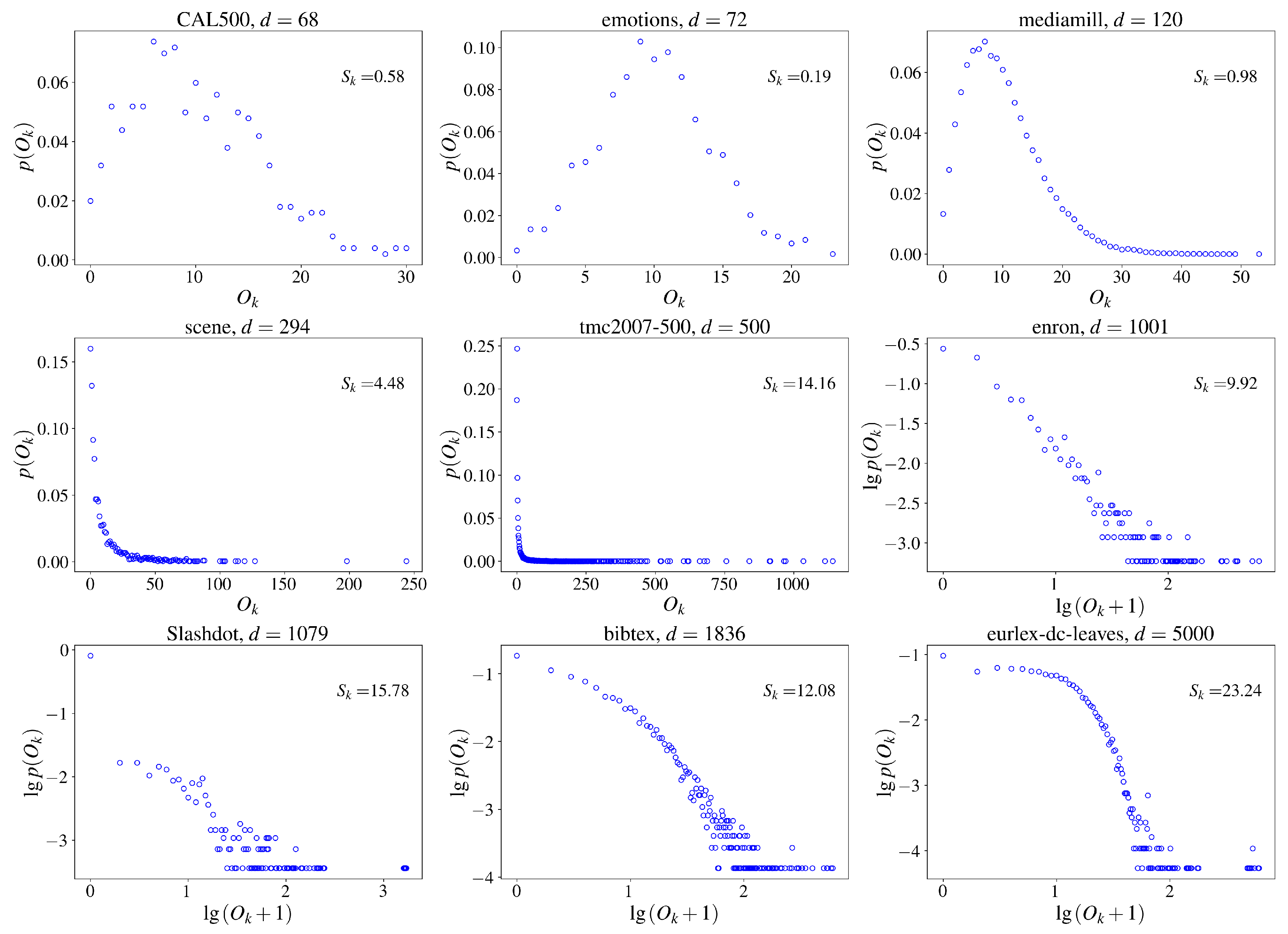
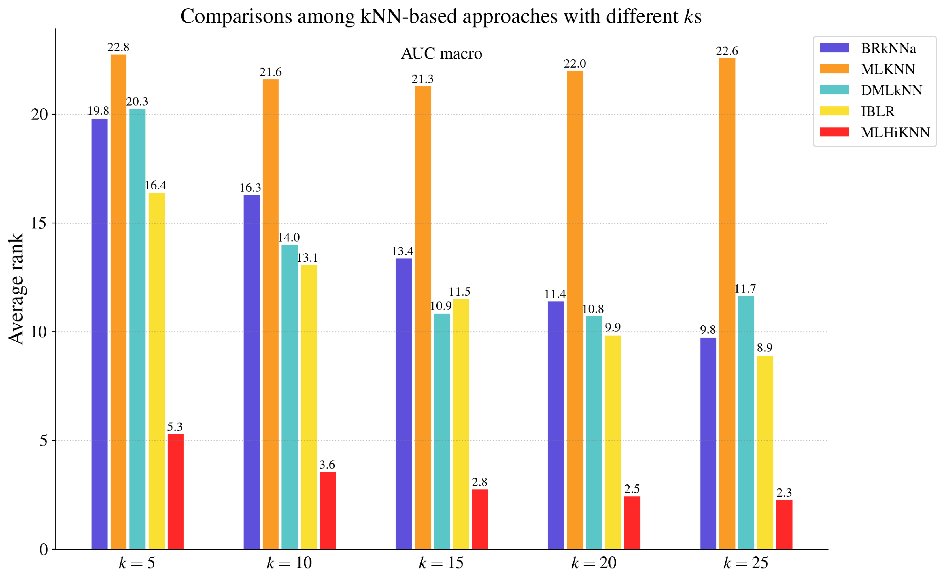
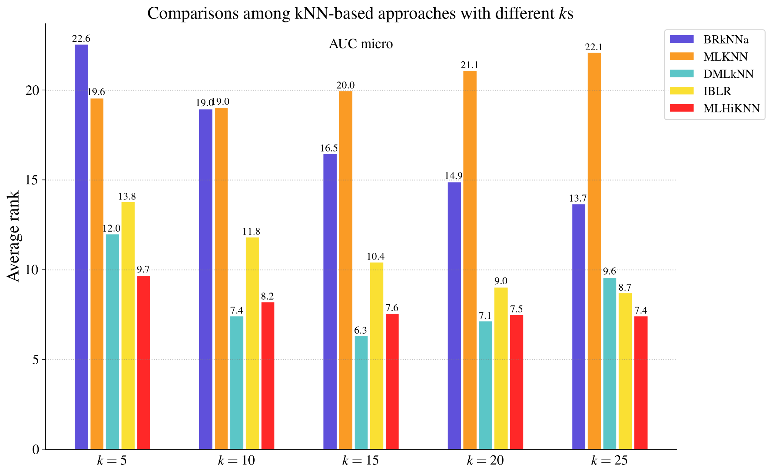
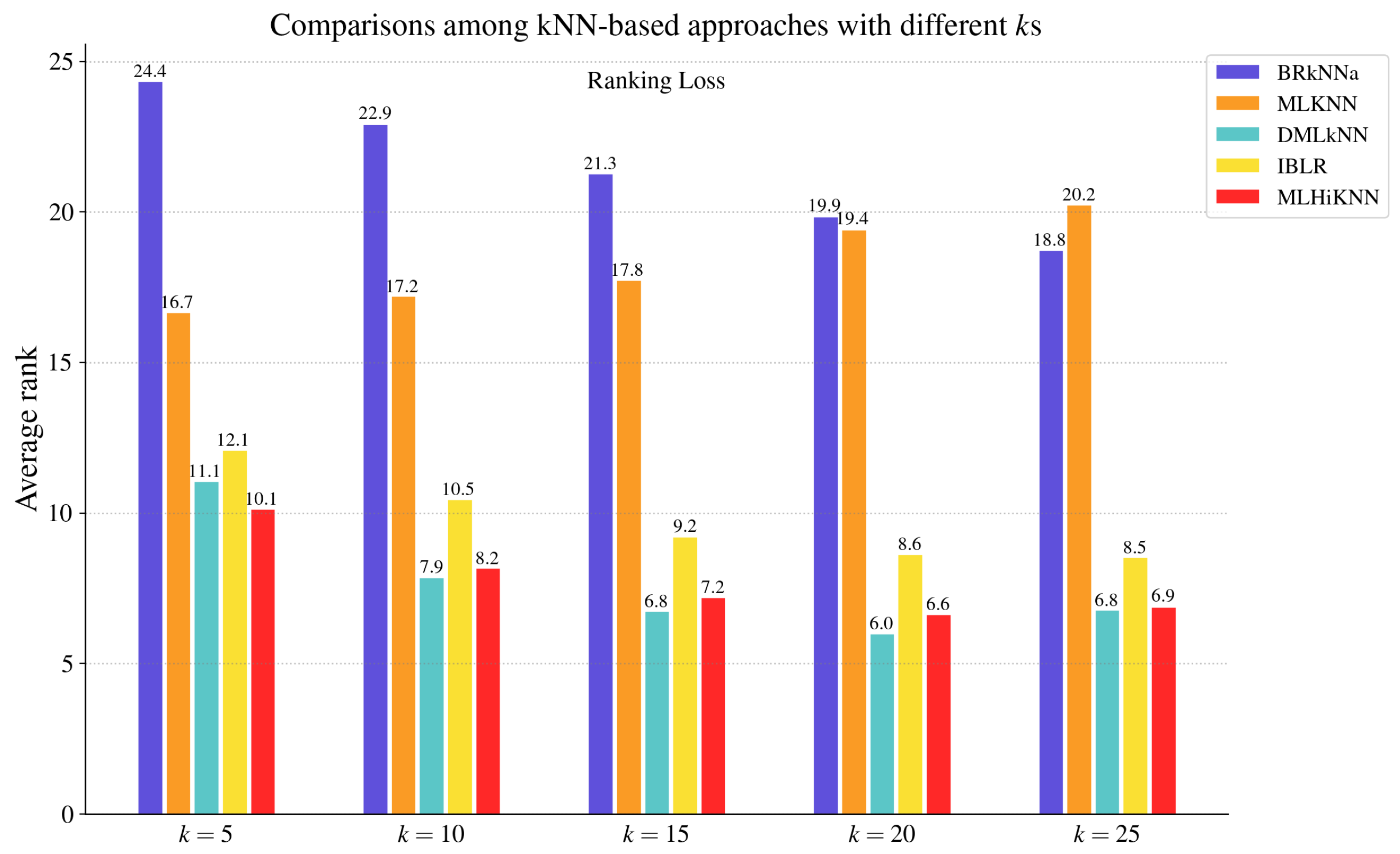
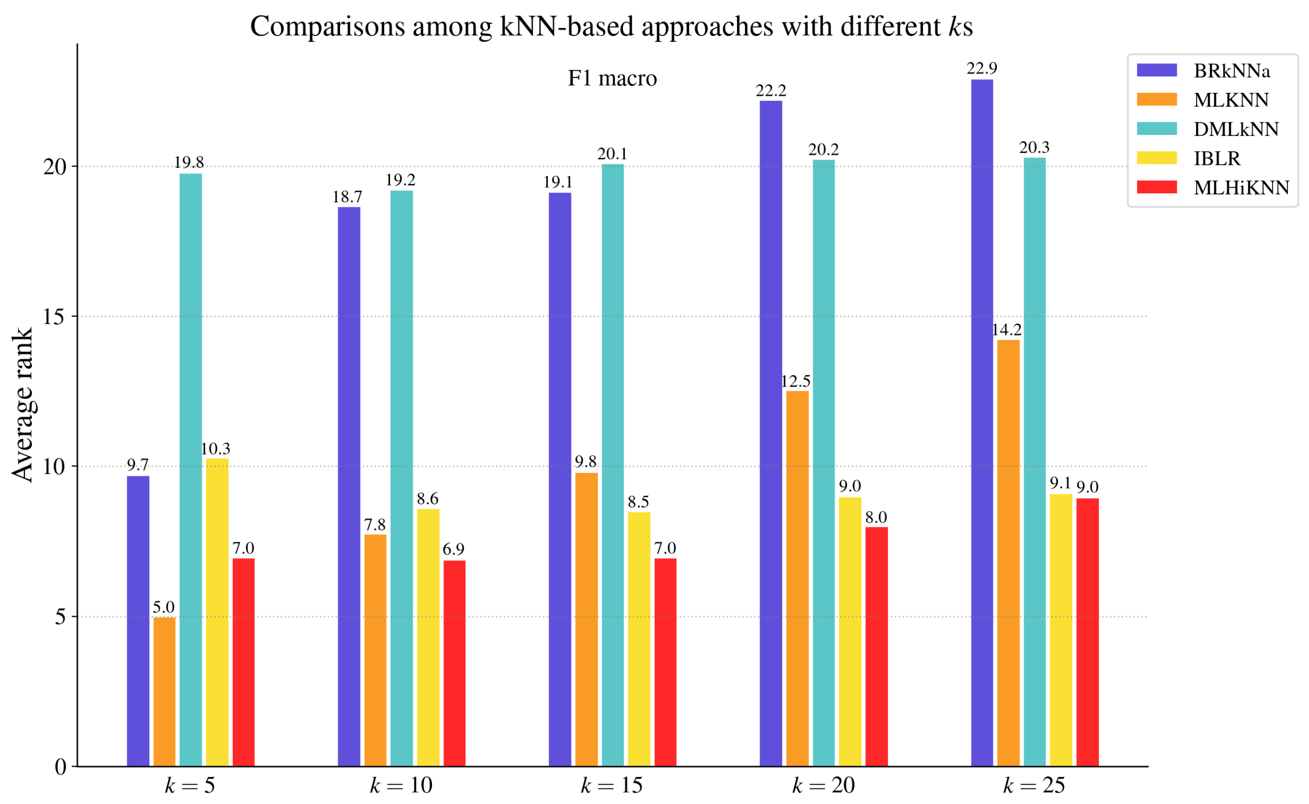
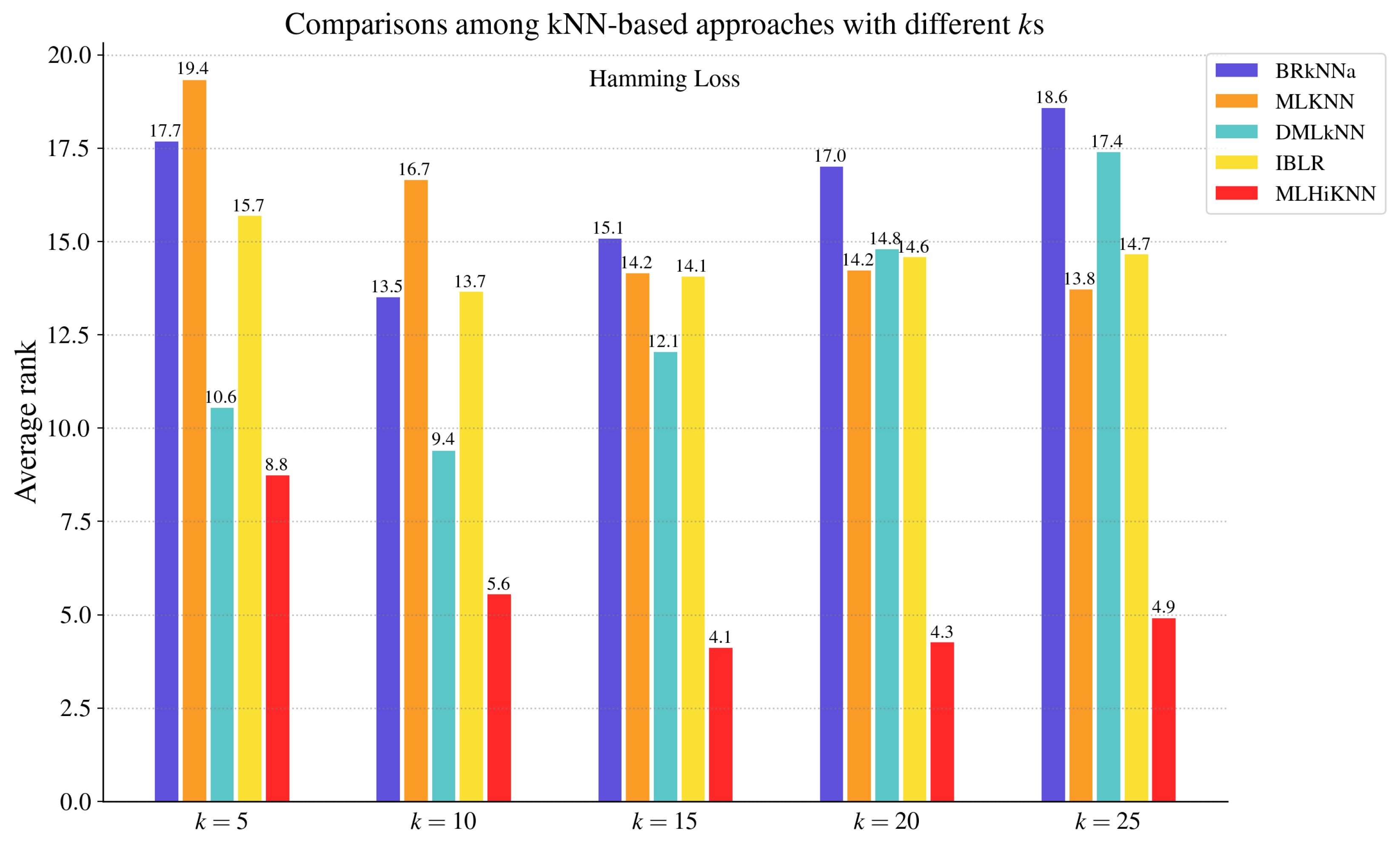
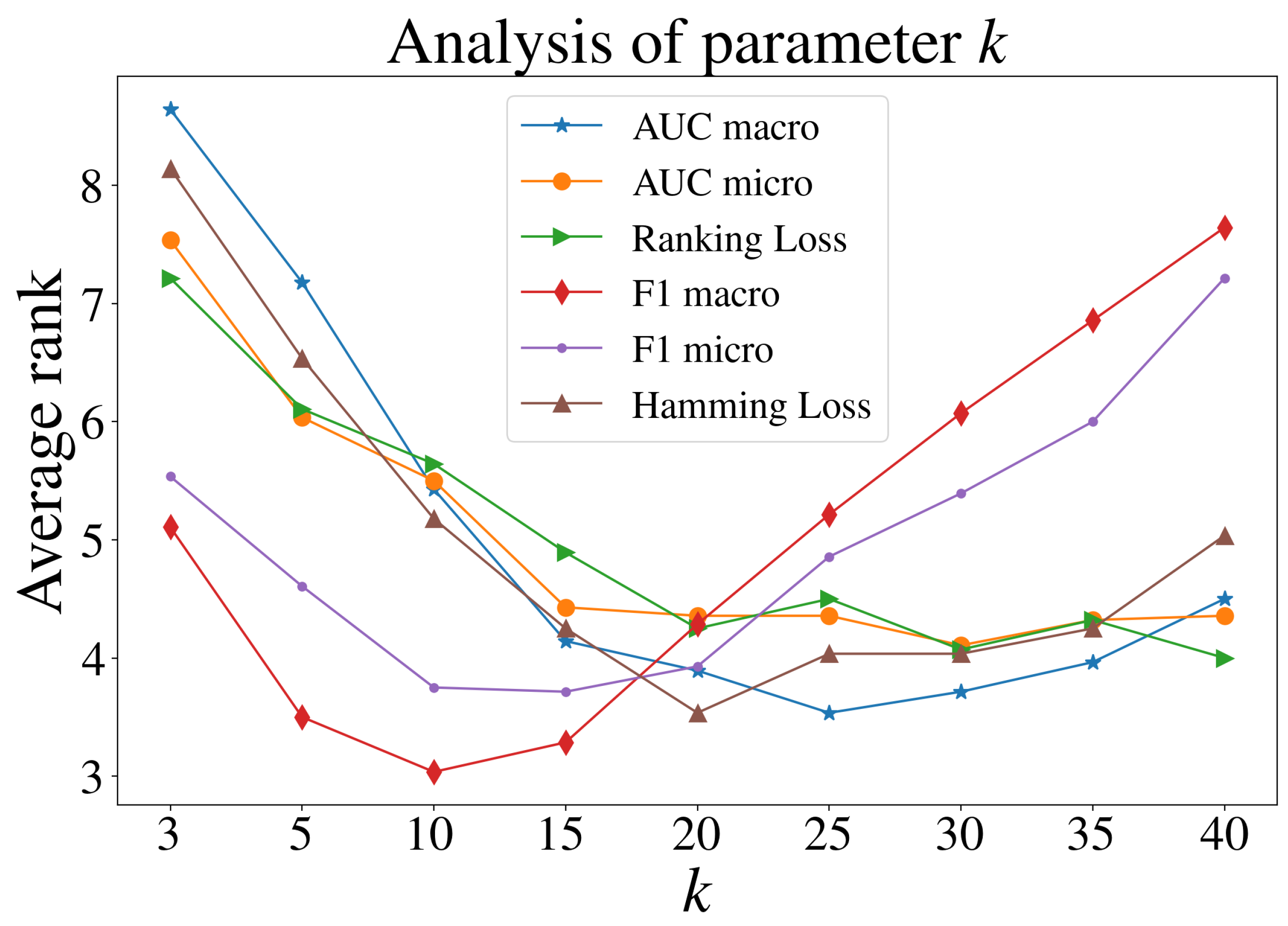
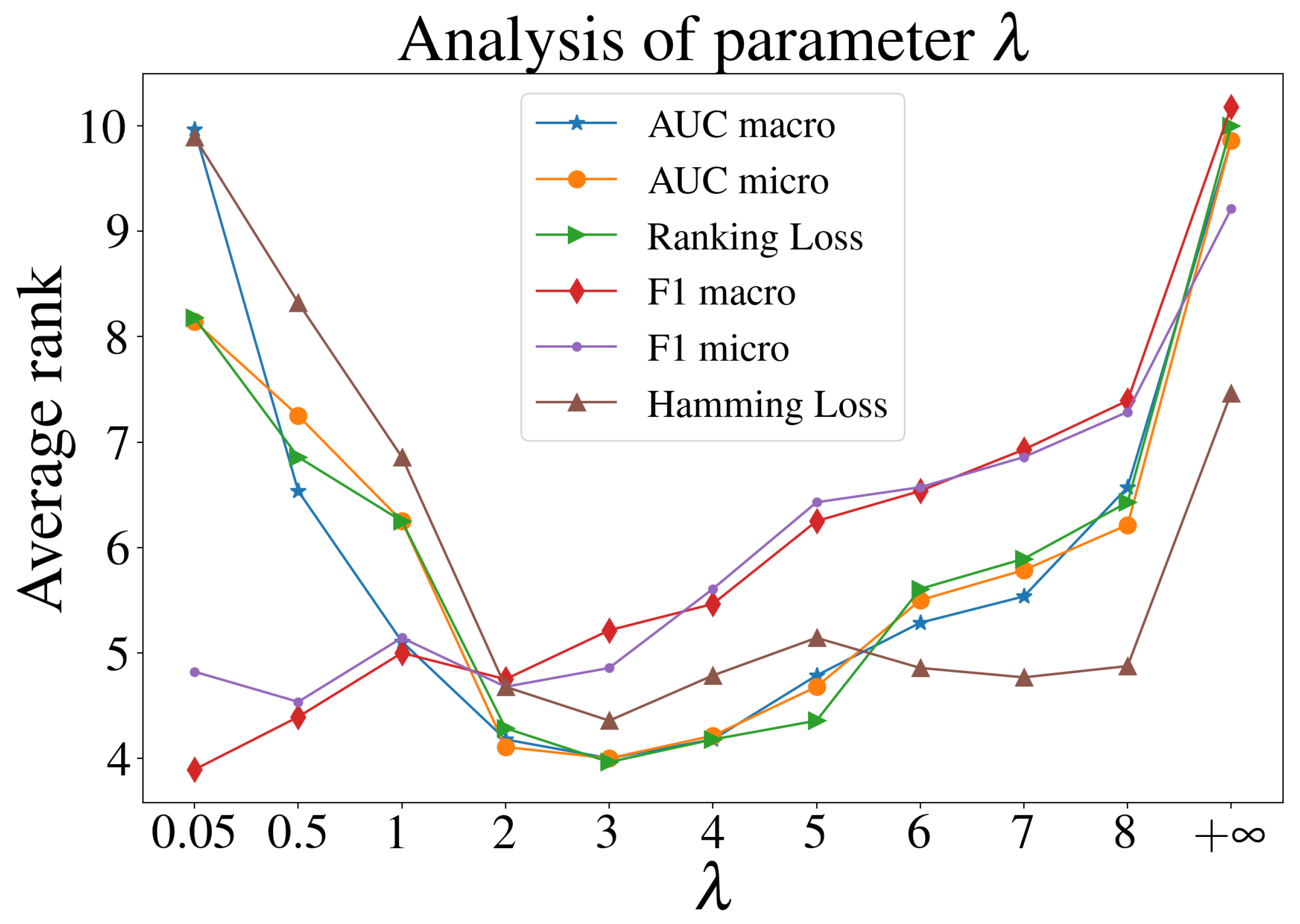
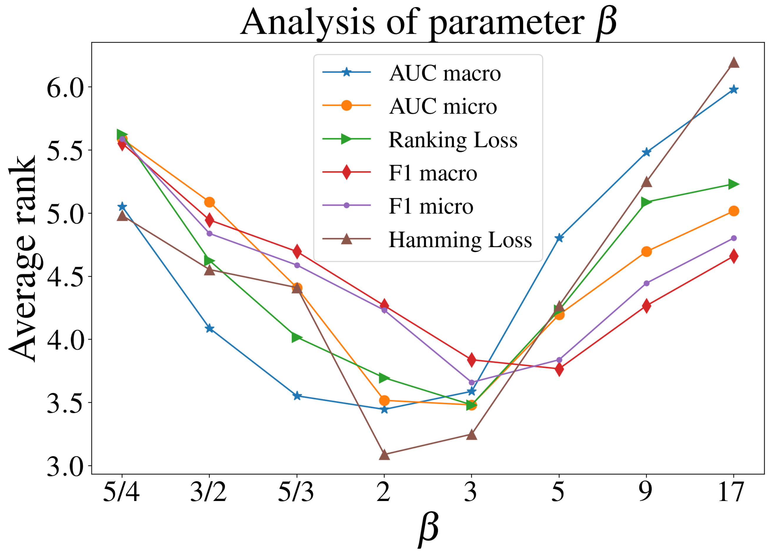
Dataset	#Samples	#Attr	#Labels	LCard	LDen	LDiv	PLDiv	${\mathit{S}}_{\mathit{k}}$	${\mathit{H}}_{\mathbf{occ}}^{\mathit{k}}$	${\mathit{A}}_{\mathbf{occ}}^{\mathit{k}}$	Domain
birds	327	260	12	1.76	0.15	92	0.28	-0.22	0.01	0.0000	audio
CAL500	502	68	124	25.06	0.20	502	1.00	0.58	0.12	0.0000	music
emotions	593	72	6	1.87	0.31	27	0.05	0.19	0.01	0.0000	music
genbase	662	1186	13	1.13	0.09	14	0.02	−0.06	0.00	0.0000	biology
LLOG	1429	100	75	16.28	0.22	1213	0.85	11.38	1.00	0.9685	text
enron	1702	1001	35	3.28	0.09	675	0.40	9.92	0.65	0.0000	text
scene	2407	294	6	1.07	0.18	15	0.01	4.48	0.52	0.0000	image
yeast	2417	103	14	4.24	0.30	198	0.08	1.55	0.26	0.0000	biology
Slashdot	2771	53	12	1.18	0.10	52	0.02	15.78	0.89	0.7694	text
corel5k	4985	499	153	3.18	0.02	2626	0.53	24.64	0.79	0.0000	images
rcv1subset1	6000	472	80	2.84	0.04	977	0.16	8.21	0.42	0.0010	text
rcv1subset2	6000	472	83	2.60	0.03	903	0.15	5.28	0.41	0.0047	text
rcv1subset3	6000	472	83	2.58	0.03	899	0.15	6.17	0.41	0.0048	text
rcv1subset4	6000	472	82	2.46	0.03	762	0.13	5.42	0.40	0.0053	text
rcv1subset5	6000	472	84	2.61	0.03	902	0.15	6.02	0.41	0.0097	text
bibtex	7395	184	159	2.40	0.02	2856	0.39	12.08	0.52	0.0368	text
Arts	7484	462	24	1.65	0.07	595	0.08	17.88	0.44	0.0345	text
Health	9205	612	21	1.64	0.08	314	0.03	14.84	0.44	0.0214	text
Business	11,204	438	25	1.60	0.06	221	0.02	26.53	0.54	0.1252	text
Education	12,016	550	27	1.46	0.05	488	0.04	12.24	0.43	0.0137	text
Computers	12,434	681	27	1.50	0.06	403	0.03	18.04	0.46	0.0314	text
Entertainment	12,730	640	17	1.41	0.08	317	0.02	23.59	0.45	0.0324	text
Recreation	12,828	606	22	1.43	0.06	530	0.04	28.08	0.46	0.0677	text
Society	14,512	636	26	1.67	0.06	1053	0.07	18.50	0.45	0.0300	text
eurlex-dc-l (In the tables of this paper, the dataset eurlex-dc-leaves is denoted by eurlex-dc-l for short)	18,593	250	215	1.26	0.01	1115	0.06	23.24	0.32	0.0575	text
eurlex-sm	19,282	250	136	2.20	0.02	2314	0.12	3.68	0.28	0.0200	text
tmc2007-500	28,596	500	22	2.22	0.10	1172	0.04	14.16	0.62	0.0002	text
mediamill	42,177	120	101	4.56	0.05	6554	0.16	0.98	0.16	0.0000	video

Many metrics have been proposed to evaluate the generalization performance of MLC algorithms. Generally, existing multi-label metrics can be categorized into two groups, example-based and label-based metrics, according to the way they deal with multiple labels. Example-based metrics first perform evaluations on each test example by considering all possible labels and then return the average value over all test instances. In contrast, label-based metrics first perform evaluations on each class label and then return the averaged value across all possible labels. In addition, similar to single-label settings, multi-label metrics can also be categorized into classification and ranking metrics according to the perspective from which the performance is measured. Importantly, different metrics vary in their sensitivity to majority and minority labels. Example-based metrics tend to be more sensitive to majority labels. For those measured from the classification perspective, majority labels contribute more often to per-instance calculations, since these labels are more likely to appear in the true label set of each instance and are also more frequently predicted by models that do not aggressively optimize recall for minority labels. For these ranking-based metrics, such as Ranking Loss, majority labels participate more often in pairwise comparisons against irrelevant labels because they are more likely to be included in the label set of each instance. Label-based metrics can be computed using two different averaging strategies: micro-averaging and macro-averaging. Micro-averaging aggregates predictions across all labels and instances and is also more influenced by majority labels. For example, in classification metrics, majority labels typically have higher overall counts of true positives and false negatives. Meanwhile, minority labels often yield smaller numbers of true positives and false positives, particularly when the classifier does not aggressively optimize their recall. Ranking-based metric AUC micro compares all relevant and irrelevant instance–label pairs. Majority labels generate more relevant instance–label pairs and thus dominate the set of relevant and irrelevant comparisons. In contrast, macro-averaging computes metric values independently for each label and then returns the averaged value. This strategy provides greater sensitivity to the performance of minority labels than micro-averaging and example-based metrics. To ensure a comprehensive evaluation of the classifier performance, we employed six evaluation metrics in our experimental analysis, including AUC macro, AUC micro, Ranking Loss, F1 macro, F1 micro, and Hamming Loss. The categorization of these metrics is summarized in Table 2.

Table 2. Categories of the metrics used in the evaluation.

Perspective	Macro-Averaging	Micro-Averaging	Example-Based
Ranking	AUC macro	AUC micro	Ranking Loss
Classification	F1 macro	F1 micro	Hamming Loss

4.1.2. Compared Approaches

To validate the effectiveness of the proposed method, we experimentally compared MLHiKNN with some well-established approaches, including nine MLC algorithms and three hubness reduction techniques. The compared MLC algorithms include BR [14], CC [17], ECC [17], RAkEL [18], RAkELd [18], BRkNNa [5], MLKNN [6], DMLkNN [7], and IBLR [8]. We employed the implementations in the Scikit-multilearn [67] library for BRkNNa and MLKNN and the implementations in the MULAN [63] library for the other seven approaches. For BR, CC, ECC, RAkEL, and RAkELd, we used C4.5 as the base classifier and employed its implementation J48 on the WEKA [68] platform. For ECC, we followed the default parameter settings. Specifically, ECC employed sampling with replacement to create the data for each base model in the ensemble. Each model was trained on 100% of the instances. The number of models was set to 10. For RAkEL and RAkELd, the size of the label subsets was set to 3. The number of models was determined adaptively based on the number of labels and the subset size, following the default settings. For the kNN-based methods, BRkNNa, MLKNN, DMLkNN, IBLR, and MLHiKNN, the number of nearest neighbors to take into account, k, was set to 20 based on both the prior literature and empirical results. Previous studies typically adopted k values ranging from 8 to 12 for MLKNN, from 8 to 10 for DMLkNN, and from 1 to 30 for BRkNNa, and used $k=10$ for IBLR. In our experiments, we further evaluated each method with $k\in \{5,10,15,20,25\}$ and observed that the optimal performance tended to occur when k was between 15 and 25 for BRkNNa, DMLkNN, and IBLR, and between 5 and 20 for MLKNN, in terms of AUC macro. To ensure a fair and consistent comparison across methods, we fixed $k=20$ for all methods and also report comparison results for these kNN-based methods under each k value in Figure 2, Figure 3, Figure 4, Figure 5, Figure 6 and Figure 7. The smooth parameter was set to 1.0 for MLKNN and DMLkNN. Other parameters followed the default parameter settings. For the proposed approach, MLHiKNN, $\lambda$ and $\beta$ were set to 3 and 2, respectively.

Figure 2. The average rank across all the datasets of each combination of algorithm and k out of twenty-five combinations in terms of AUC macro.

Figure 3. The average rank across all the datasets of each combination of algorithm and k out of twenty-five combinations in terms of AUC micro.

Figure 4. The average rank across all the datasets of each combination of algorithm and k out of twenty-five combinations in terms of Ranking Loss.

Figure 5. The average rank across all the datasets of each combination of algorithm and k out of twenty-five combinations in terms of F1 macro.

Figure 6. The average rank across all the datasets of each combination of algorithm and k out of twenty-five combinations in terms of F1 micro.

Figure 7. The average rank across all the datasets of each combination of algorithm and k out of twenty-five combinations in terms of Hamming Loss.

The compared hubness reduction techniques include local dissimilarity (DSL) [34], local scaling (LS) [40,41], and mutual proximity (MP) [40,41]. For the three hubness reduction techniques, we employed their implementations in the Scikit-hubness [69] library. For DSL and LS, k was set to be 20. For MP, the Gaussian method was used to model the distance distributions. Other parameters all followed the default settings.

To compare the hubness reduction techniques with MLHiKNN, we incorporated these techniques into BRkNNa and MLKNN, respectively, resulting in two groups of methods. They are hubness-reduced BRkNNa approaches (Algorithm 4), including BRkNNa-dsl, BRkNNa-ls, BRkNNa-mp, and hubness-reduced MLKNN approaches (Algorithm 5), including MLKNN-dsl, MLKNN-ls, and MLKNN-mp. Compared with the hubness-reduced BRkNNa approaches, the hubness-reduced MLKNN approaches also need to search for the k nearest neighbors for each training example with hubness reduction techniques to compute the posterior probabilities in the training process.

Algorithm 4 Hubness-reduced BRkNNa.

Input:

D: training set;

$P_h$: parameters needed for BRkNNa and the hubness reduction technique;

$D_{test}$: testing set.

Output:

${\widehat{Y}}_{test}$: label predictions of testing set. 1: for each instance t in $D_{test}$ do 2:       $G_{hbr}(t,D)\leftarrow$ Compute the transformed pairwise distances or relations between t and all examples in D with a hubness reduction technique based on the dataset $\{t\cup D\}$ 3:       $D_k\left(t\right)\leftarrow$ Identify the kNNs of t based on the relations in $G_{hbr}(t,D)$ 4:       ${\widehat{y}}_t\leftarrow$ Predict the label set of t with BRkNNa taking $D_k\left(t\right)$ as the kNNs 5: end for 6: return ${\widehat{Y}}_{test}\leftarrow \left\{{\widehat{y}}_t\right|t\in D_{test}\}$

Algorithm 5 Hubness-reduced MLKNN.

Input:

D: training set;

$P_h$: parameters needed for MLKNN and the hubness reduction technique;

$D_{test}$: testing set.

Output:

${\widehat{Y}}_{test}$: label predictions of testing set.   1: Compute the prior probabilities as performed with MLKNN   2: for each instance x in D do   3:       $G_{hbr}(x,D)\leftarrow$ Compute the transformed pairwise distances or relations between x and all examples in D with a hubness reduction technique based on the training set D   4:       $D_k\left(x\right)\leftarrow$ Identify the kNNs of x based on the relations in $G_{hbr}(x,D)$   5: end for   6: Compute the posterior probabilities as performed by MLKNN based on the neighboring relations in $\left\{D_k\left(x\right)\right|x\in D\}$   7: for each instance t in $D_{test}$ do   8:       $G_{hbr}(t,D)\leftarrow$ Compute the transformed pairwise distances or relations between t and all examples in D with a hubness reduction technique based on the dataset $\{t\cup D\}$   9:       $D_k\left(t\right)\leftarrow$ Identify the kNNs of t based on the relations in $G_{hbr}(t,D)$ 10:       ${\widehat{y}}_t\leftarrow$ Predict the label set of t with the prior and posterior probabilities as performed by MLKNN, taking $D_k\left(t\right)$ as the kNNs 11: end for 12: return ${\widehat{Y}}_{test}\leftarrow \left\{{\widehat{y}}_t\right|t\in D_{test}\}$

4.2. Comparisons with MLC Algorithms

In this subsection, we first report the experimental results of MLHiKNN and the nine MLC algorithms under the parameter settings mentioned in the previous subsection. Then, we report the comparison results among MLHiKNN and the four kNN-based MLC algorithms, BRkNNa, MLKNN, DMLkNN, and IBLR, under different settings of the parameter k. Table 3 shows the performance in terms of AUC macro of the compared MLC algorithms on each dataset. Each result contains the mean performance and the standard deviation across ten testing sets. For each dataset, the rank on the mean performance of each algorithm is enclosed in parentheses. For each dataset, the performance of the top-ranked algorithm is marked with •. For each algorithm, the average rank across all the datasets is shown in the second line from the bottom, with the best average rank shown in bold. The last line shows the win, tie, and loss counts of each algorithm, which were obtained by a pairwise Wilcoxon signed-rank test between each pair of algorithms on each dataset across the performance on ten testing sets. The significance level was set to 0.05. Specifically, a win (loss) was counted for an algorithm if it performed significantly better (worse) than another algorithm on a dataset. Otherwise, a tie was recorded. For brevity, the experimental results of the compared MLC algorithms on the other five metrics, AUC micro, Ranking Loss, F1 macro, F1 micro, and Hamming Loss, are shown in Table A2, Table A3, Table A4, Table A5 and Table A6. Meanwhile, the average ranks of these algorithms on each metric are summarized in Table 4 for ease of viewing, with the best average rank in each case shown in bold. As Table 3 shows, the proposed method MLHiKNN is top-ranked on 26 out of 28 benchmark datasets on AUC macro. MLHiKNN also achieves the best average rank, the highest win counts, and the lowest loss counts on AUC macro. For the other five metrics, MLHiKNN achieves the best average rank on AUC micro, Ranking Loss, and Hamming Loss, shares the third-best average rank with RAkELd on F1 macro, and ranks fifth on average based on F1 micro. In terms of F1 macro, RAkEL and BR achieve the first- and second-best ranks. In terms of F1 micro, RAkEL, ECC, BR, and RAkELd obtain the highest four average ranks. Meanwhile, MLHiKNN outperforms the other four kNN-based MLC algorithms on all metrics.

Table 3. The performance of nine compared MLC algorithms and MLHiKNN on AUC macro. The best average rank is shown in bold. For each dataset, the performance of the top-ranked algorithm is marked with •.

Dataset	AUC Macro
	BR	CC	ECC	RAkEL	RAkELd	BRkNNa	MLKNN	DMLkNN	IBLR	MLHiKNN
birds	0.624(9) ± 0.030	0.625(8) ± 0.020	0.753(1) ± 0.017 •	0.723(3) ± 0.016	0.651(7) ± 0.014	0.702(4) ± 0.016	0.606(10) ± 0.019	0.684(6) ± 0.021	0.691(5) ± 0.017	0.728(2) ± 0.030
CAL500	0.511(9) ± 0.005	0.508(10) ± 0.005	0.537(3) ± 0.006	0.527(5) ± 0.004	0.513(8) ± 0.003	0.543(2) ± 0.006	0.515(7) ± 0.004	0.530(4) ± 0.003	0.516(6) ± 0.008	0.571(1) ± 0.006 •
emotions	0.690(8) ± 0.018	0.680(10) ± 0.016	0.818(4) ± 0.008	0.793(6) ± 0.009	0.689(9) ± 0.014	0.834(3) ± 0.005	0.723(7) ± 0.013	0.805(5) ± 0.009	0.836(2) ± 0.010	0.846(1) ± 0.005 •
genbase	0.989(8) ± 0.010	0.987(9) ± 0.014	0.996(4) ± 0.005	0.997(2) ± 0.004	0.994(7) ± 0.008	0.996(5) ± 0.004	0.963(10) ± 0.013	0.998(1) ± 0.001 •	0.995(6) ± 0.006	0.997(3) ± 0.003
LLOG	0.526(9) ± 0.002	0.525(10) ± 0.004	0.539(6) ± 0.006	0.531(8) ± 0.002	0.536(7) ± 0.005	0.598(4) ± 0.006	0.588(5) ± 0.006	0.602(3) ± 0.006	0.602(2) ± 0.006	0.603(1) ± 0.006 •
enron	0.580(9) ± 0.008	0.576(10) ± 0.004	0.646(2) ± 0.005	0.631(5) ± 0.005	0.585(8) ± 0.009	0.627(6) ± 0.012	0.596(7) ± 0.011	0.634(4) ± 0.014	0.641(3) ± 0.017	0.676(1) ± 0.012 •
scene	0.761(8) ± 0.015	0.752(10) ± 0.014	0.921(5) ± 0.004	0.894(7) ± 0.003	0.760(9) ± 0.011	0.937(3) ± 0.003	0.898(6) ± 0.007	0.932(4) ± 0.004	0.940(2) ± 0.003	0.944(1) ± 0.002 •
yeast	0.569(8) ± 0.006	0.562(10) ± 0.007	0.641(5) ± 0.005	0.625(6) ± 0.004	0.562(9) ± 0.010	0.685(3) ± 0.005	0.583(7) ± 0.006	0.671(4) ± 0.006	0.692(2) ± 0.006	0.711(1) ± 0.006 •
Slashdot	0.560(8) ± 0.019	0.581(6) ± 0.021	0.535(10) ± 0.014	0.550(9) ± 0.010	0.595(5) ± 0.019	0.680(3) ± 0.017	0.563(7) ± 0.033	0.671(4) ± 0.034	0.682(2) ± 0.035	0.723(1) ± 0.021 •
corel5k	0.522(6) ± 0.002	0.516(10) ± 0.002	0.520(8) ± 0.002	0.516(9) ± 0.001	0.522(7) ± 0.002	0.582(4) ± 0.004	0.569(5) ± 0.004	0.587(3) ± 0.007	0.603(2) ± 0.008	0.690(1) ± 0.005 •
rcv1subset1	0.642(9) ± 0.008	0.614(10) ± 0.005	0.728(6) ± 0.004	0.661(7) ± 0.005	0.649(8) ± 0.011	0.819(4) ± 0.006	0.766(5) ± 0.006	0.835(2) ± 0.005	0.834(3) ± 0.005	0.891(1) ± 0.004 •
rcv1subset2	0.645(9) ± 0.007	0.595(10) ± 0.009	0.721(6) ± 0.005	0.652(8) ± 0.003	0.653(7) ± 0.006	0.819(3) ± 0.008	0.770(5) ± 0.007	0.841(2) ± 0.006	0.810(4) ± 0.007	0.888(1) ± 0.005 •
rcv1subset3	0.635(9) ± 0.007	0.584(10) ± 0.008	0.718(6) ± 0.005	0.646(8) ± 0.004	0.648(7) ± 0.006	0.816(3) ± 0.007	0.767(5) ± 0.007	0.834(2) ± 0.008	0.816(4) ± 0.005	0.880(1) ± 0.004 •
rcv1subset4	0.643(8) ± 0.012	0.600(10) ± 0.007	0.714(6) ± 0.004	0.642(9) ± 0.005	0.652(7) ± 0.010	0.816(3) ± 0.006	0.769(5) ± 0.006	0.840(2) ± 0.007	0.811(4) ± 0.007	0.887(1) ± 0.007 •
rcv1subset5	0.640(9) ± 0.010	0.594(10) ± 0.007	0.714(6) ± 0.005	0.647(8) ± 0.003	0.649(7) ± 0.008	0.810(4) ± 0.006	0.758(5) ± 0.005	0.834(2) ± 0.006	0.812(3) ± 0.008	0.873(1) ± 0.005 •
bibtex	0.639(7) ± 0.007	0.634(8) ± 0.007	0.661(6) ± 0.003	0.617(10) ± 0.004	0.626(9) ± 0.006	0.794(4) ± 0.003	0.754(5) ± 0.004	0.807(2) ± 0.003	0.806(3) ± 0.005	0.886(1) ± 0.001 •
Arts	0.598(8) ± 0.005	0.594(9) ± 0.007	0.650(5) ± 0.004	0.631(6) ± 0.004	0.601(7) ± 0.004	0.695(3) ± 0.009	0.545(10) ± 0.007	0.685(4) ± 0.009	0.704(2) ± 0.013	0.730(1) ± 0.009 •
Health	0.687(8) ± 0.008	0.686(9) ± 0.009	0.731(5) ± 0.006	0.713(6) ± 0.005	0.687(7) ± 0.011	0.745(3) ± 0.008	0.606(10) ± 0.008	0.737(4) ± 0.010	0.754(2) ± 0.011	0.778(1) ± 0.009 •
Business	0.609(7) ± 0.010	0.597(9) ± 0.007	0.641(5) ± 0.009	0.628(6) ± 0.005	0.609(8) ± 0.010	0.701(3) ± 0.009	0.589(10) ± 0.008	0.704(2) ± 0.009	0.699(4) ± 0.011	0.752(1) ± 0.007 •
Education	0.601(9) ± 0.011	0.607(7) ± 0.011	0.648(5) ± 0.005	0.635(6) ± 0.006	0.606(8) ± 0.015	0.698(2) ± 0.009	0.595(10) ± 0.006	0.683(4) ± 0.010	0.696(3) ± 0.014	0.748(1) ± 0.014 •
Computers	0.618(8) ± 0.007	0.602(10) ± 0.009	0.674(5) ± 0.008	0.657(6) ± 0.007	0.620(7) ± 0.010	0.707(4) ± 0.006	0.611(9) ± 0.004	0.710(3) ± 0.006	0.715(2) ± 0.009	0.750(1) ± 0.005 •
Entertainment	0.654(9) ± 0.010	0.661(8) ± 0.011	0.724(5) ± 0.007	0.694(6) ± 0.005	0.677(7) ± 0.013	0.743(4) ± 0.005	0.581(10) ± 0.008	0.749(3) ± 0.004	0.754(2) ± 0.006	0.782(1) ± 0.004 •
Recreation	0.648(8) ± 0.008	0.647(9) ± 0.009	0.709(5) ± 0.006	0.678(6) ± 0.006	0.658(7) ± 0.011	0.752(3) ± 0.006	0.559(10) ± 0.012	0.751(4) ± 0.010	0.762(2) ± 0.009	0.788(1) ± 0.009 •
Society	0.593(8) ± 0.006	0.585(9) ± 0.004	0.636(5) ± 0.004	0.622(6) ± 0.004	0.594(7) ± 0.006	0.675(3) ± 0.005	0.554(10) ± 0.007	0.673(4) ± 0.005	0.683(2) ± 0.006	0.707(1) ± 0.006 •
eurlex-dc-l	0.635(8) ± 0.005	0.630(10) ± 0.006	0.676(6) ± 0.002	0.637(7) ± 0.004	0.634(9) ± 0.005	0.820(2) ± 0.005	0.785(4) ± 0.005	0.798(3) ± 0.005	0.774(5) ± 0.006	0.900(1) ± 0.004 •
eurlex-sm	0.686(8) ± 0.005	0.683(10) ± 0.007	0.736(6) ± 0.003	0.707(7) ± 0.004	0.685(9) ± 0.006	0.852(2) ± 0.005	0.814(5) ± 0.004	0.842(3) ± 0.006	0.841(4) ± 0.006	0.908(1) ± 0.003 •
tmc2007-500	0.761(10) ± 0.005	0.765(9) ± 0.006	0.847(5) ± 0.003	0.837(6) ± 0.003	0.770(8) ± 0.010	0.863(4) ± 0.002	0.799(7) ± 0.003	0.888(3) ± 0.002	0.891(2) ± 0.002	0.920(1) ± 0.002 •
mediamill	0.596(8) ± 0.004	0.577(10) ± 0.004	0.638(7) ± 0.003	0.647(6) ± 0.003	0.584(9) ± 0.006	0.747(4) ± 0.003	0.704(5) ± 0.003	0.781(2) ± 0.003	0.761(3) ± 0.005	0.824(1) ± 0.002 •
average rank	8.29	9.29	5.29	6.57	7.64	3.39	7.18	3.18	3.07	1.11
win/tie/loss	29/30/193	17/20/215	128/8/116	88/18/146	49/32/171	175/19/58	75/8/169	181/16/55	184/22/46	244/7/1

Table 4. The average ranks across all the datasets of nine compared MLC algorithms and MLHiKNN on each metric. The best average rank in each case is shown in bold.

Metric	BR	CC	ECC	RAkEL	RAkELd	BRkNNa	MLKNN	DMLkNN	IBLR	MLHiKNN
AUC macro	8.29	9.29	5.29	6.57	7.64	3.39	7.18	3.18	3.07	1.11
AUC micro	6.43	7.86	6.18	8.18	8.39	4.14	6.39	2.29	2.89	2.25
Ranking Loss	5.86	6.57	7.79	9.04	8.21	5.75	5.11	2.18	2.61	1.89
F1 macro	3.79	5.00	5.07	2.89	4.39	9.29	6.64	8.68	4.86	4.39
F1 micro	4.21	5.54	2.93	2.57	5.00	8.82	6.21	8.46	5.86	5.39
Hamming Loss	5.93	8.32	2.89	3.89	7.64	6.11	5.54	5.46	6.50	2.71

To statistically analyze the MLC algorithms across all these datasets, the Friedman test was conducted at a significance level of 0.05. The results on each metric are shown in Table 5. Then, the pairwise Wilcoxon signed-rank test was employed for each pair of these algorithms across all the datasets as the post hoc test [70]. Meanwhile, the significant level of 0.05 was corrected by the Bonferroni method to control the family-wise Type-I error. The results are shown in Table 6, Table 7, Table 8, Table 9, Table 10 and Table 11. In each table, the $i,j$ entry is the p-value of the pairwise Wilcoxon signed-rank test, whose alternative hypothesis is that the i-th method performs significantly better than the j-th method based on their performance on all the datasets. The p-values less than the corrected significant level are filled in gray. As shown in Table 5, the test statistic of the Friedman test is larger than the Critical Value for each metric. So, the null hypothesis of the Friedman test is rejected in terms of each metric. According to Table 6, Table 7, Table 8, Table 9, Table 10 and Table 11, MLHiKNN significantly outperforms all the other nine MLC algorithms in terms of AUC macro. For the other two ranking-based metrics, AUC micro and Ranking Loss, MLHiKNN performs significantly better than all compared algorithms, except for DMLkNN and IBLR on both metrics, and BRkNNa on AUC micro. For the three classification-based metrics, MLHiKNN significantly outperforms BRkNNa and DMLkNN in all cases. In terms of Hamming Loss, it also achieves significantly better performance than all other compared algorithms, except for ECC and RAkEL. Moreover, no algorithm significantly outperforms MLHiKNN on any of the evaluated metrics. These experimental results indicate that MLHiKNN is highly competitive among the compared MLC algorithms.

Table 5. The Friedman test statistics $F_F$ for comparisons among ten MLC algorithms BR, CC, ECC, RAkEL, RAkELd, BRkNNa, MLKNN, DMLkNN, IBLR, and MLHiKNN. The critical value is calculated at a significance level of 0.05. # Algorithms and # Datasets denote the number of algorithms and the number of datasets, respectively.

Metric	${\mathit{F}}_{\mathit{F}}$	# Algorithms	# Datasets	Critical Value
AUC macro	200.743	10	28	1.919
AUC micro	161.135
Ranking Loss	180.210
F1 macro	118.442
F1 micro	114.732
Hamming Loss	95.447

Table 6. p-values of the post hoc tests for the comparison among ten MLC algorithms in terms of AUC macro. The $i,j$ entry corresponds to the test whose alternative hypothesis is that the i-th method performs significantly better than the j-th method. The corrected significance level is 5.56 $\times {10}^{-4}$. The p-values less than the corrected significant level are filled in gray.

AUC Macro	BR	CC	ECC	RAkEL	RAkELd	BRkNNa	MLKNN	DMLkNN	IBLR	MLHiKNN
BR	-	3.23 $\times {10}^{-4}$	1.000	1.000	0.996	1.000	0.986	1.000	1.000	1.000
CC	1.000	-	1.000	1.000	1.000	1.000	0.992	1.000	1.000	1.000
ECC	5.22 $\times {10}^{-8}$	1.23 $\times {10}^{-7}$	-	5.10 $\times {10}^{-7}$	9.42 $\times {10}^{-7}$	1.000	0.113	1.000	1.000	1.000
RAkEL	4.70 $\times {10}^{-6}$	5.10 $\times {10}^{-7}$	1.000	-	2.36 $\times {10}^{-4}$	1.000	0.685	1.000	1.000	1.000
RAkELd	0.004	3.28 $\times {10}^{-7}$	1.000	1.000	-	1.000	0.977	1.000	1.000	1.000
BRkNNa	3.73 $\times {10}^{-9}$	3.73 $\times {10}^{-9}$	2.84 $\times {10}^{-6}$	7.08 $\times {10}^{-8}$	3.73 $\times {10}^{-9}$	-	3.73 $\times {10}^{-9}$	0.685	0.959	1.000
MLKNN	0.015	0.009	0.891	0.323	0.024	1.000	-	1.000	1.000	1.000
DMLkNN	3.73 $\times {10}^{-9}$	3.73 $\times {10}^{-9}$	1.03 $\times {10}^{-5}$	7.08 $\times {10}^{-8}$	3.73 $\times {10}^{-9}$	0.323	3.73 $\times {10}^{-9}$	-	0.669	1.000
IBLR	3.73 $\times {10}^{-9}$	3.73 $\times {10}^{-9}$	2.84 $\times {10}^{-6}$	9.31 $\times {10}^{-8}$	3.73 $\times {10}^{-9}$	0.043	1.12 $\times {10}^{-8}$	0.339	-	1.000
MLHiKNN	3.73 $\times {10}^{-9}$	3.73 $\times {10}^{-9}$	1.86 $\times {10}^{-8}$	7.45 $\times {10}^{-9}$	3.73 $\times {10}^{-9}$	3.73 $\times {10}^{-9}$	3.73 $\times {10}^{-9}$	1.12 $\times {10}^{-8}$	3.73 $\times {10}^{-9}$	-

Table 7. p-values of the post hoc tests for the comparison among ten MLC algorithms in terms of AUC micro. The $i,j$ entry corresponds to the test whose alternative hypothesis is that the i-th method performs significantly better than the j-th method. The corrected significance level is 5.56 $\times {10}^{-4}$. The p-values less than the corrected significant level are filled in gray.

AUC Micro	BR	CC	ECC	RAkEL	RAkELd	BRkNNa	MLKNN	DMLkNN	IBLR	MLHiKNN
BR	-	1.03 $\times {10}^{-5}$	0.619	0.045	3.28 $\times {10}^{-7}$	1.000	0.967	1.000	1.000	1.000
CC	1.000	-	0.980	0.323	0.024	1.000	0.997	1.000	1.000	1.000
ECC	0.390	0.021	-	1.12 $\times {10}^{-8}$	1.09 $\times {10}^{-4}$	1.000	0.760	1.000	1.000	1.000
RAkEL	0.957	0.685	1.000	-	0.478	1.000	0.999	1.000	1.000	1.000
RAkELd	1.000	0.977	1.000	0.531	-	1.000	1.000	1.000	1.000	1.000
BRkNNa	1.14 $\times {10}^{-6}$	9.31 $\times {10}^{-8}$	3.98 $\times {10}^{-6}$	9.31 $\times {10}^{-8}$	1.86 $\times {10}^{-8}$	-	1.83 $\times {10}^{-5}$	1.000	0.999	0.998
MLKNN	0.035	0.004	0.247	0.001	1.19 $\times {10}^{-5}$	1.000	-	1.000	1.000	1.000
DMLkNN	3.73 $\times {10}^{-9}$	3.73 $\times {10}^{-9}$	3.28 $\times {10}^{-7}$	1.86 $\times {10}^{-8}$	3.73 $\times {10}^{-9}$	6.47 $\times {10}^{-6}$	3.73 $\times {10}^{-9}$	-	0.055	0.746
IBLR	1.14 $\times {10}^{-6}$	2.61 $\times {10}^{-8}$	1.83 $\times {10}^{-5}$	9.42 $\times {10}^{-7}$	1.86 $\times {10}^{-8}$	7.08 $\times {10}^{-4}$	6.47 $\times {10}^{-6}$	0.948	-	0.937
MLHiKNN	1.12 $\times {10}^{-8}$	3.73 $\times {10}^{-9}$	1.23 $\times {10}^{-7}$	1.86 $\times {10}^{-8}$	3.73 $\times {10}^{-9}$	0.002	1.14 $\times {10}^{-6}$	0.261	0.066	-

Table 8. p-values of the post hoc tests for the comparison among ten MLC algorithms in terms of Ranking Loss. The $i,j$ entry corresponds to the test whose alternative hypothesis is that the i-th method performs significantly better than the j-th method. The corrected significance level is 5.56 $\times {10}^{-4}$. The p-values less than the corrected significant level are filled in gray.

Ranking Loss	BR	CC	ECC	RAkEL	RAkELd	BRkNNa	MLKNN	DMLkNN	IBLR	MLHiKNN
BR	-	0.001	0.002	2.11 $\times {10}^{-5}$	3.73 $\times {10}^{-9}$	0.813	0.990	1.000	1.000	1.000
CC	0.999	-	0.010	3.60 $\times {10}^{-5}$	8.61 $\times {10}^{-5}$	0.957	0.998	1.000	1.000	1.000
ECC	0.998	0.990	-	1.12 $\times {10}^{-8}$	0.940	1.000	1.000	1.000	1.000	1.000
RAkEL	1.000	1.000	1.000	-	0.999	1.000	1.000	1.000	1.000	1.000
RAkELd	1.000	1.000	0.063	6.45 $\times {10}^{-4}$	-	1.000	1.000	1.000	1.000	1.000
BRkNNa	0.193	0.045	5.22 $\times {10}^{-8}$	7.45 $\times {10}^{-9}$	3.16 $\times {10}^{-5}$	-	0.842	1.000	1.000	1.000
MLKNN	0.010	0.002	4.70 $\times {10}^{-6}$	5.22 $\times {10}^{-8}$	9.31 $\times {10}^{-8}$	0.164	-	1.000	1.000	1.000
DMLkNN	1.12 $\times {10}^{-8}$	7.45 $\times {10}^{-9}$	7.45 $\times {10}^{-9}$	7.45 $\times {10}^{-9}$	7.45 $\times {10}^{-9}$	7.45 $\times {10}^{-9}$	3.73 $\times {10}^{-9}$	-	0.031	0.558
IBLR	2.05 $\times {10}^{-7}$	1.86 $\times {10}^{-8}$	1.60 $\times {10}^{-7}$	2.61 $\times {10}^{-8}$	3.73 $\times {10}^{-9}$	4.70 $\times {10}^{-6}$	7.57 $\times {10}^{-6}$	0.970	-	0.950
MLHiKNN	7.45 $\times {10}^{-9}$	3.73 $\times {10}^{-9}$	3.73 $\times {10}^{-9}$	3.73 $\times {10}^{-9}$	3.73 $\times {10}^{-9}$	3.73 $\times {10}^{-9}$	7.71 $\times {10}^{-7}$	0.451	0.052	-

Table 9. p-values of the post hoc tests for the comparison among ten MLC algorithms in terms of F1 macro. The $i,j$ entry corresponds to the test whose alternative hypothesis is that the i-th method performs significantly better than the j-th method. The corrected significance level is 5.56 $\times {10}^{-4}$. The p-values less than the corrected significant level are filled in gray.

F1 Macro	BR	CC	ECC	RAkEL	RAkELd	BRkNNa	MLKNN	DMLkNN	IBLR	MLHiKNN
BR	-	0.013	0.024	0.998	0.063	9.31 $\times {10}^{-8}$	4.66 $\times {10}^{-5}$	9.42 $\times {10}^{-7}$	0.060	0.187
CC	0.988	-	0.137	1.000	0.899	4.10 $\times {10}^{-7}$	9.34 $\times {10}^{-4}$	8.83 $\times {10}^{-6}$	0.169	0.451
ECC	0.977	0.868	-	1.000	0.972	1.60 $\times {10}^{-7}$	1.22 $\times {10}^{-4}$	3.28 $\times {10}^{-7}$	0.323	0.339
RAkEL	0.002	1.22 $\times {10}^{-4}$	6.77 $\times {10}^{-5}$	-	6.77 $\times {10}^{-5}$	3.73 $\times {10}^{-8}$	5.10 $\times {10}^{-7}$	7.08 $\times {10}^{-8}$	0.007	0.055
RAkELd	0.940	0.105	0.030	1.000	-	2.61 $\times {10}^{-7}$	8.61 $\times {10}^{-5}$	2.00 $\times {10}^{-6}$	0.060	0.219
BRkNNa	1.000	1.000	1.000	1.000	1.000	-	1.000	0.999	1.000	1.000
MLKNN	1.000	0.999	1.000	1.000	1.000	2.61 $\times {10}^{-8}$	-	3.73 $\times {10}^{-9}$	1.000	0.999
DMLkNN	1.000	1.000	1.000	1.000	1.000	5.86 $\times {10}^{-4}$	1.000	-	1.000	1.000
IBLR	0.943	0.836	0.685	0.993	0.943	1.86 $\times {10}^{-8}$	4.83 $\times {10}^{-4}$	3.73 $\times {10}^{-9}$	-	0.701
MLHiKNN	0.819	0.558	0.669	0.948	0.788	2.61 $\times {10}^{-8}$	0.001	1.86 $\times {10}^{-8}$	0.307	-

Table 10. p-values of the post hoc tests for the comparison among ten MLC algorithms in terms of F1 micro. The $i,j$ entry corresponds to the test whose alternative hypothesis is that the i-th method performs significantly better than the j-th method. The corrected significance level is 5.56 $\times {10}^{-4}$. The p-values less than the corrected significant level are filled in gray.

F1 Micro	BR	CC	ECC	RAkEL	RAkELd	BRkNNa	MLKNN	DMLkNN	IBLR	MLHiKNN
BR	-	0.003	0.996	1.000	4.66 $\times {10}^{-5}$	8.83 $\times {10}^{-6}$	0.003	6.77 $\times {10}^{-5}$	0.010	0.063
CC	0.997	-	1.000	1.000	0.794	1.71 $\times {10}^{-4}$	0.050	0.003	0.127	0.276
ECC	0.004	6.47 $\times {10}^{-6}$	-	0.153	0.003	3.98 $\times {10}^{-6}$	1.91 $\times {10}^{-4}$	6.47 $\times {10}^{-6}$	0.006	0.001
RAkEL	2.42 $\times {10}^{-5}$	6.30 $\times {10}^{-7}$	0.853	-	5.10 $\times {10}^{-7}$	7.71 $\times {10}^{-7}$	7.64 $\times {10}^{-5}$	9.42 $\times {10}^{-7}$	2.12 $\times {10}^{-4}$	0.001
RAkELd	1.000	0.212	0.997	1.000	-	5.29 $\times {10}^{-5}$	0.020	4.83 $\times {10}^{-4}$	0.043	0.101
BRkNNa	1.000	1.000	1.000	1.000	1.000	-	1.000	0.997	1.000	1.000
MLKNN	0.998	0.953	1.000	1.000	0.981	2.61 $\times {10}^{-7}$	-	1.86 $\times {10}^{-8}$	0.478	0.965
DMLkNN	1.000	0.997	1.000	1.000	1.000	0.003	1.000	-	1.000	1.000
IBLR	0.991	0.877	0.995	1.000	0.959	1.59 $\times {10}^{-5}$	0.531	1.60 $\times {10}^{-7}$	-	0.953
MLHiKNN	0.940	0.732	0.999	0.999	0.903	1.67 $\times {10}^{-6}$	0.037	1.14 $\times {10}^{-6}$	0.050	-

Table 11. p-values of the post hoc tests for the comparison among ten MLC algorithms in terms of Hamming Loss. The $i,j$ entry corresponds to the test whose alternative hypothesis is that the i-th method performs significantly better than the j-th method. The corrected significance level is 5.56 $\times {10}^{-4}$. The p-values less than the corrected significant level are filled in gray.

Hamming Loss	BR	CC	ECC	RAkEL	RAkELd	BRkNNa	MLKNN	DMLkNN	IBLR	MLHiKNN
BR	-	2.61 $\times {10}^{-8}$	1.000	1.000	1.38 $\times {10}^{-6}$	0.788	0.934	0.948	0.132	1.000
CC	1.000	-	1.000	1.000	0.963	0.997	1.000	1.000	0.895	1.000
ECC	2.38 $\times {10}^{-6}$	3.73 $\times {10}^{-9}$	-	1.19 $\times {10}^{-5}$	3.98 $\times {10}^{-6}$	0.013	0.013	0.016	0.004	0.753
RAkEL	6.30 $\times {10}^{-7}$	3.73 $\times {10}^{-9}$	1.000	-	3.73 $\times {10}^{-9}$	0.199	0.451	0.407	0.006	0.899
RAkELd	1.000	0.039	1.000	1.000	-	0.967	0.999	0.999	0.760	1.000
BRkNNa	0.219	0.003	0.988	0.807	0.035	-	0.940	0.940	0.381	1.000
MLKNN	0.069	3.96 $\times {10}^{-4}$	0.988	0.558	8.52 $\times {10}^{-4}$	0.063	-	0.373	0.158	1.000
DMLkNN	0.055	2.92 $\times {10}^{-4}$	0.985	0.602	6.45 $\times {10}^{-4}$	0.063	0.636	-	0.158	1.000
IBLR	0.873	0.109	0.996	0.994	0.247	0.627	0.847	0.847	-	1.000
MLHiKNN	5.29 $\times {10}^{-5}$	7.71 $\times {10}^{-7}$	0.254	0.105	8.83 $\times {10}^{-6}$	7.08 $\times {10}^{-8}$	2.38 $\times {10}^{-6}$	2.84 $\times {10}^{-6}$	2.11 $\times {10}^{-5}$	-

Further, since MLHiKNN is a k-nearest neighbor approach, we also compared MLHiKNN with the four kNN-based MLC algorithms, BRkNNa, MLKNN, DMLkNN, and IBLR, under different settings of k. Experiments were conducted on the five algorithms with parameter k set to be each value in $\{5,10,15,20,25\}$. Hence, there were a total of twenty-five combinations of algorithm and k. For each combination of algorithm and k, its average rank across all the datasets out of the twenty-five combinations is reported in Figure 2, Figure 3, Figure 4, Figure 5, Figure 6 and Figure 7 in terms of each metric. Thus, it is convenient to observe the performance rank differences among the five algorithms under each setting of k and among the combinations of one algorithm with different ks. Then, we try to answer three questions based on the results of these experiments. First, how does parameter k influence the performance of the kNN-based MLC algorithms? Second, how does the proposed method MLHiKNN perform compared with the other four kNN-based algorithms? Third, how does the performance of these algorithms vary across different metrics? According to Figure 2, Figure 3, Figure 4, Figure 5, Figure 6 and Figure 7, the following observations can be made to answer the above questions. First, in terms of the three ranking-based metrics, AUC macro, AUC micro, and Ranking Loss, the average performance of all algorithms generally improves at first and then tends to stabilize as k increases from 5 to 25 in steps of 5, except for MLKNN on all three metrics and DMLkNN on AUC micro. Naturally, considering more nearest neighbors can bring more information for predicting labels. However, the performance of these algorithms does not always exhibit the same tendency in terms of the three classification-based metrics as that in terms of the ranking-based metrics as k increases. One reason for that lies in the class imbalance. For MLKNN, the performance decreases as k increases from 5 to 25 in terms of Ranking Loss, F1 macro, and F1 micro. The reason is that MLKNN makes a prediction for each possible label l following an MAP principle based on the number of examples with label l among the kNNs. A larger k leads to more possible values of such a number. Thus, on average, there are fewer instances for each value of this number, since the total number of training examples is fixed. As a result, the posterior probability estimation may be less accurate for some values of this number due to the lack of examples. The second observation is that MLHiKNN achieves the best average rank on each value of k in terms of AUC macro and Hamming Loss. For AUC micro, MLHiKNN achieves the best average rank on two values of k and the second-best rank on three values of k. For Ranking Loss, MLHiKNN achieves the best average rank on one value of k and the second-best rank on four values of k. In terms of F1 macro and F1 micro, it achieves the best average rank on four values of k and the second-best rank on one value of k. These results indicate the competitive performance of MLHiKNN on different values of k compared with the other kNN-based MLC algorithms. Third, the performance of these algorithms varies greatly across different metrics. For example, MLKNN achieves better average ranks on F1 macro than on AUC macro. DMLkNN achieves better average ranks on Ranking Loss than on F1 macro. IBLR ranks better on average on F1 macro than on Hamming Loss. These differences in performance across the metrics show the different focuses of these algorithms. Specifically, minority classes have more influence on macro-averaging metrics than on micro-averaging metrics and example-based metrics. These metrics also have the difference of classification and ranking. Note that MLHiKNN always achieves the best or second-best average rank in terms of each metric. It shows the effectiveness of MLHiKNN across different focuses.

4.3. Comparisons with Hubness Reduction Techniques

In this subsection, we report the experimental results of the hubness-reduced MLC approaches, introduced in Section 4.1.2. The performance on each dataset is shown in Table 12, Table A7, Table A8, Table A9, Table A10 and Table A11. Meanwhile, the average ranks of the algorithms in terms of each metric are organized into Figure 8 for ease of viewing. For statistical analysis, the Friedman test and post hoc pairwise Wilcoxon signed-rank test were also employed. The significance level was set to 0.05. The results of the Friedman test are shown in Table A12. The p-values of the post hoc test are shown in Table 13, Table A13, Table A14, Table A15, Table A16 and Table A17. The representations of the contents in these tables follow those introduced in Section 4.2. We try to answer two questions based on the results reported in this subsection. First, do the hubness reduction techniques improve the performance of BRkNNa and MLKNN? Second, how does MLHiKNN perform compared with the hubness-reduced MLC approaches? For the first question, both BRkNNa-dsl and BRkNNa-ls achieve better average ranks than BRkNNa on all six metrics, indicating that incorporating the two hubness reduction techniques, DSL and LS, leads to performance improvements for BRkNNa. For MLKNN, the three variants, MLKNN-dsl, MLKNN-ls, and MLKNN-mp, all achieve worse average ranks than MLKNN across all these metrics, except for Hamming Loss. This is because MLKNN is less affected by the hubness phenomenon than BRkNNa, owing to its MAP strategy. It might not benefit much from hubness reduction. Instead, the distance transformation in the hubness reduction techniques, which is based on the distribution estimated using training examples, introduces the negative effects of the error between the estimated distribution and true distribution to MLKNN in its training and predicting processes. For the second question, MLHiKNN achieves the best average rank in terms of each metric. Meanwhile, it performs significantly better than all the compared approaches discussed in this subsection in terms of AUC macro, Ranking Loss, and Hamming Loss. For F1 macro and F1 micro, it also achieves significantly better performance than all compared approaches, except for MLKNN. In terms of AUC micro, MLHiKNN outperforms both MLKNN and its three variants, MLKNN-dsl, MLKNN-ls, and MLKNN-mp. It shows MLHiKNN is highly competitive compared with the hubness-reduced MLC approaches.

Table 12. The performance of the algorithms for hubness reduction technique comparisons on AUC macro. The best average rank is shown in bold. For each dataset, the performance of the top-ranked algorithm is marked with •.

Dataset	AUC Macro
	BRkNNa	BRkNNa-dsl	BRkNNa-ls	BRkNNa-mp	MLKNN	MLKNN-dsl	MLKNN-ls	MLKNN-mp	MLHiKNN
birds	0.702(4) ± 0.016	0.701(5) ± 0.028	0.728(1) ± 0.009 •	0.708(3) ± 0.010	0.606(6) ± 0.019	0.490(7) ± 0.025	0.472(8) ± 0.025	0.452(9) ± 0.032	0.728(2) ± 0.030
CAL500	0.543(4) ± 0.006	0.539(5) ± 0.007	0.545(3) ± 0.004	0.546(2) ± 0.006	0.515(6) ± 0.004	0.494(7) ± 0.005	0.494(8) ± 0.004	0.491(9) ± 0.004	0.571(1) ± 0.006 •
emotions	0.834(4) ± 0.005	0.830(5) ± 0.008	0.845(2) ± 0.007	0.842(3) ± 0.006	0.723(6) ± 0.013	0.707(7) ± 0.015	0.705(8) ± 0.016	0.701(9) ± 0.014	0.846(1) ± 0.005 •
genbase	0.996(4) ± 0.004	0.996(2) ± 0.004	0.996(3) ± 0.004	0.990(5) ± 0.006	0.963(6) ± 0.013	0.773(7) ± 0.042	0.771(8) ± 0.052	0.627(9) ± 0.080	0.997(1) ± 0.003 •
LLOG	0.598(2) ± 0.006	0.595(3) ± 0.006	0.594(5) ± 0.005	0.595(3) ± 0.006	0.588(6) ± 0.006	0.549(7) ± 0.020	0.512(9) ± 0.026	0.520(8) ± 0.019	0.603(1) ± 0.006 •
enron	0.627(4) ± 0.012	0.638(3) ± 0.012	0.644(2) ± 0.011	0.616(5) ± 0.009	0.596(6) ± 0.011	0.439(7) ± 0.015	0.434(8) ± 0.012	0.431(9) ± 0.010	0.676(1) ± 0.012 •
scene	0.937(5) ± 0.003	0.940(4) ± 0.002	0.945(1) ± 0.003 •	0.944(2) ± 0.003	0.898(6) ± 0.007	0.879(7) ± 0.016	0.879(8) ± 0.014	0.877(9) ± 0.018	0.944(3) ± 0.002
yeast	0.685(4) ± 0.005	0.663(5) ± 0.006	0.689(2) ± 0.004	0.689(3) ± 0.004	0.583(6) ± 0.006	0.522(9) ± 0.007	0.529(8) ± 0.011	0.531(7) ± 0.012	0.711(1) ± 0.006 •
Slashdot	0.680(5) ± 0.017	0.690(3) ± 0.020	0.700(2) ± 0.012	0.688(4) ± 0.015	0.563(6) ± 0.033	0.405(9) ± 0.031	0.409(8) ± 0.038	0.433(7) ± 0.029	0.723(1) ± 0.021 •
corel5k	0.582(5) ± 0.004	0.626(2) ± 0.007	0.625(4) ± 0.007	0.626(3) ± 0.008	0.569(6) ± 0.004	0.415(7) ± 0.007	0.414(8) ± 0.007	0.412(9) ± 0.006	0.690(1) ± 0.005 •
rcv1subset1	0.819(5) ± 0.006	0.844(3) ± 0.005	0.845(2) ± 0.004	0.823(4) ± 0.005	0.766(6) ± 0.006	0.396(7) ± 0.016	0.393(8) ± 0.016	0.367(9) ± 0.007	0.891(1) ± 0.004 •
rcv1subset2	0.819(5) ± 0.008	0.843(2) ± 0.007	0.840(3) ± 0.007	0.823(4) ± 0.006	0.770(6) ± 0.007	0.363(8) ± 0.014	0.376(7) ± 0.012	0.328(9) ± 0.016	0.888(1) ± 0.005 •
rcv1subset3	0.816(4) ± 0.007	0.838(3) ± 0.005	0.840(2) ± 0.011	0.815(5) ± 0.007	0.767(6) ± 0.007	0.360(7) ± 0.015	0.358(8) ± 0.023	0.336(9) ± 0.021	0.880(1) ± 0.004 •
rcv1subset4	0.816(5) ± 0.006	0.837(2) ± 0.007	0.837(3) ± 0.007	0.823(4) ± 0.009	0.769(6) ± 0.006	0.380(8) ± 0.010	0.387(7) ± 0.010	0.344(9) ± 0.010	0.887(1) ± 0.007 •
rcv1subset5	0.810(4) ± 0.006	0.830(2) ± 0.004	0.827(3) ± 0.006	0.809(5) ± 0.006	0.758(6) ± 0.005	0.324(8) ± 0.014	0.370(7) ± 0.021	0.316(9) ± 0.015	0.873(1) ± 0.005 •
bibtex	0.794(5) ± 0.003	0.813(4) ± 0.003	0.826(2) ± 0.002	0.814(3) ± 0.003	0.754(6) ± 0.004	0.352(9) ± 0.012	0.400(8) ± 0.007	0.432(7) ± 0.007	0.886(1) ± 0.001 •
Arts	0.695(4) ± 0.009	0.699(2) ± 0.010	0.696(3) ± 0.008	0.677(5) ± 0.007	0.545(6) ± 0.007	0.339(9) ± 0.008	0.343(8) ± 0.008	0.357(7) ± 0.007	0.730(1) ± 0.009 •
Health	0.745(4) ± 0.008	0.750(2) ± 0.008	0.746(3) ± 0.004	0.714(5) ± 0.008	0.606(6) ± 0.008	0.324(9) ± 0.013	0.346(7) ± 0.007	0.326(8) ± 0.007	0.778(1) ± 0.009 •
Business	0.701(4) ± 0.009	0.705(3) ± 0.008	0.718(2) ± 0.006	0.679(5) ± 0.007	0.589(6) ± 0.008	0.328(8) ± 0.007	0.317(9) ± 0.005	0.342(7) ± 0.007	0.752(1) ± 0.007 •
Education	0.698(4) ± 0.009	0.701(2) ± 0.009	0.701(3) ± 0.008	0.675(5) ± 0.010	0.595(6) ± 0.006	0.331(9) ± 0.011	0.336(8) ± 0.014	0.352(7) ± 0.011	0.748(1) ± 0.014 •
Computers	0.707(4) ± 0.006	0.711(3) ± 0.005	0.715(2) ± 0.006	0.685(5) ± 0.006	0.611(6) ± 0.004	0.319(9) ± 0.006	0.321(8) ± 0.004	0.336(7) ± 0.005	0.750(1) ± 0.005 •
Entertainment	0.743(4) ± 0.005	0.746(2) ± 0.005	0.744(3) ± 0.006	0.726(5) ± 0.008	0.581(6) ± 0.008	0.374(8) ± 0.006	0.379(7) ± 0.005	0.329(9) ± 0.008	0.782(1) ± 0.004 •
Recreation	0.752(4) ± 0.006	0.754(2) ± 0.006	0.752(3) ± 0.006	0.728(5) ± 0.005	0.559(6) ± 0.012	0.296(9) ± 0.006	0.301(8) ± 0.007	0.312(7) ± 0.006	0.788(1) ± 0.009 •
Society	0.675(4) ± 0.005	0.679(2) ± 0.005	0.677(3) ± 0.006	0.661(5) ± 0.006	0.554(6) ± 0.007	0.348(9) ± 0.005	0.350(8) ± 0.006	0.363(7) ± 0.006	0.707(1) ± 0.006 •
eurlex-dc-l	0.820(4) ± 0.005	0.822(2) ± 0.005	0.820(3) ± 0.005	0.805(5) ± 0.004	0.785(6) ± 0.005	0.296(8) ± 0.014	0.303(7) ± 0.012	0.197(9) ± 0.004	0.900(1) ± 0.004 •
eurlex-sm	0.852(3) ± 0.005	0.853(2) ± 0.004	0.852(4) ± 0.004	0.842(5) ± 0.004	0.814(6) ± 0.004	0.302(9) ± 0.010	0.303(7) ± 0.011	0.302(8) ± 0.008	0.908(1) ± 0.003 •
tmc2007-500	0.863(4) ± 0.002	0.885(2) ± 0.001	0.881(3) ± 0.002	0.858(5) ± 0.002	0.799(6) ± 0.003	0.440(7) ± 0.009	0.433(8) ± 0.012	0.374(9) ± 0.017	0.920(1) ± 0.002 •
mediamill	0.747(4) ± 0.003	0.747(5) ± 0.003	0.752(2) ± 0.003	0.752(3) ± 0.004	0.704(6) ± 0.003	0.326(7) ± 0.005	0.323(8) ± 0.005	0.322(9) ± 0.007	0.824(1) ± 0.002 •
average rank	4.14	2.95	2.64	4.16	6.00	7.93	7.82	8.25	1.11
win/tie/loss	129/21/74	158/21/45	164/27/33	127/16/81	84/0/140	19/16/189	23/21/180	16/15/193	216/7/1

Figure 8. The average rank across all the datasets of each algorithm for hubness reduction technique comparisons in terms of each metric.

Table 13. p-values of the post hoc tests for the comparisons with hubness reduction techniques in terms of AUC macro. The $i,j$ entry corresponds to the test whose alternative hypothesis is that the i-th method performs significantly better than the j-th method. The corrected significance level is 6.94 $\times {10}^{-4}$. The p-values less than the corrected significant level are filled in gray.

AUC Macro	BRkNNa	BRkNNa-dsl	BRkNNa-ls	BRkNNa-mp	MLKNN	MLKNN-dsl	MLKNN-ls	MLKNN-mp	MLHiKNN
BRkNNa	-	1.000	1.000	0.089	3.73 $\times {10}^{-9}$	3.73 $\times {10}^{-9}$	3.73 $\times {10}^{-9}$	3.73 $\times {10}^{-9}$	1.000
BRkNNa-dsl	5.32 $\times {10}^{-4}$	-	0.937	8.06 $\times {10}^{-4}$	3.73 $\times {10}^{-9}$	3.73 $\times {10}^{-9}$	3.73 $\times {10}^{-9}$	3.73 $\times {10}^{-9}$	1.000
BRkNNa-ls	4.10 $\times {10}^{-7}$	0.066	-	2.05 $\times {10}^{-7}$	3.73 $\times {10}^{-9}$	3.73 $\times {10}^{-9}$	3.73 $\times {10}^{-9}$	3.73 $\times {10}^{-9}$	1.000
BRkNNa-mp	0.915	0.999	1.000	-	3.73 $\times {10}^{-9}$	3.73 $\times {10}^{-9}$	3.73 $\times {10}^{-9}$	3.73 $\times {10}^{-9}$	1.000
MLKNN	1.000	1.000	1.000	1.000	-	3.73 $\times {10}^{-9}$	3.73 $\times {10}^{-9}$	3.73 $\times {10}^{-9}$	1.000
MLKNN-dsl	1.000	1.000	1.000	1.000	1.000	-	0.887	0.072	1.000
MLKNN-ls	1.000	1.000	1.000	1.000	1.000	0.118	-	0.050	1.000
MLKNN-mp	1.000	1.000	1.000	1.000	1.000	0.931	0.953	-	1.000
MLHiKNN	3.73 $\times {10}^{-9}$	3.73 $\times {10}^{-9}$	3.73 $\times {10}^{-8}$	7.45 $\times {10}^{-9}$	3.73 $\times {10}^{-9}$	3.73 $\times {10}^{-9}$	3.73 $\times {10}^{-9}$	3.73 $\times {10}^{-9}$	-

4.4. Ablation Analysis for MLHiKNN

To validate the effectiveness of each strategy in the proposed method, we conducted experiments on some variants of MLHiKNN for ablation analysis. MLHiKNN-g1: $g\left(x\right)$ was fixed at 1 for computing Equations (9) and (10). Thus, for each neighbor of a query instance t, its membership was either 0 or 1 according to its label. When computing its membership, the hubness information was not considered. There was no fuzziness, actually. MLHiKNN-g0: $g\left(x\right)$ was fixed at 0 for computing Equations (9) and (10). Thus, for each training example, its membership only depended on its hubness information. As a neighbor, x voted by its history k-occurrence and label k-occurrence information rather than its label. The labels of each neighbor were ignored in the kNN voting. MLHiKNN-h1: $w_h(t,x)$ was fixed at 1 for computing Equation (5). Thus, for the kNNs of a query instance, the history k-occurrence made no difference in their importance in kNN voting. The hubness weighting was removed. MLHiKNN-d1: $w_d(t,x)$ was fixed at 1 for computing Equation (5). Thus, for the kNNs of a query instance t, the distance to t made no difference in their importance in the kNN voting. The distance weighting was removed. MLHiKNN-fo: The label relevance score computed by Equation (6) was directly used for prediction without the logistic regression model. Specifically, label l was assigned to the query instance t if and only if $r^l\left(t\right)\ge 0.5$. MLHiKNN-fo is a first-order approach, accordingly. The above approaches are summarized in Table 14. The performance of MLHiKNN and each variant approach on each dataset is shown in Table 15 and Table A18, Table A19, Table A20, Table A21 and Table A22. The average ranks across all the datasets are shown in Figure 9. As the figure shows, MLHiKNN achieves the second-best average rank on F1 macro and the best average rank on the remaining five metrics. It verifies the effectiveness of each strategy in MLHiKNN.

Table 14. The variant approaches for ablation analysis.

Approach	Explanation
MLHiKNN-g1	$g\left(x\right)$ is fixed at 1 in Equations (9) and (10)
MLHiKNN-g0	$g\left(x\right)$ is fixed at 0 in Equations (9) and (10)
MLHiKNN-h1	$w_h(t,x)$ is fixed at 1 in Equation (5)
MLHiKNN-d1	$w_d(t,x)$ is fixed at 1 in Equation (5)
MLHiKNN-fo	${\widehat{y}}_t^l=\left\{\begin{array}{cc}1\hfill & \mathrm{if}{r}^l\left(t\right)\ge 0.5\hfill \\ 0\hfill & \mathrm{otherwise}\hfill \end{array}\right.$

Table 15. The performance of MLHiKNN and the variant approaches in terms of AUC macro. The best average rank is shown in bold. For each dataset, the performance of the top-ranked algorithm is marked with •.

Dataset	AUC Macro
	MLHiKNN-g1	MLHiKNN-g0	MLHiKNN-h1	MLHiKNN-d1	MLHiKNN-fo	MLHiKNN
birds	0.728(3) ± 0.031	0.723(4) ± 0.033	0.718(6) ± 0.032	0.719(5) ± 0.028	0.755(1) ± 0.019 •	0.728(2) ± 0.030
CAL500	0.561(5) ± 0.006	0.564(4) ± 0.007	0.573(1) ± 0.006 •	0.571(3) ± 0.005	0.558(6) ± 0.004	0.571(2) ± 0.006
emotions	0.845(2) ± 0.009	0.840(6) ± 0.006	0.845(3) ± 0.007	0.844(4) ± 0.007	0.843(5) ± 0.006	0.846(1) ± 0.005 •
genbase	0.996(6) ± 0.004	0.997(5) ± 0.003	0.997(3) ± 0.003	0.998(2) ± 0.003	0.998(1) ± 0.002 •	0.997(4) ± 0.003
LLOG	0.603(5) ± 0.006	0.603(1) ± 0.006 •	0.603(2) ± 0.006	0.603(3) ± 0.006	0.603(6) ± 0.006	0.603(4) ± 0.006
enron	0.663(6) ± 0.011	0.671(4) ± 0.007	0.670(5) ± 0.010	0.673(2) ± 0.012	0.672(3) ± 0.011	0.676(1) ± 0.012 •
scene	0.945(1) ± 0.003 •	0.942(6) ± 0.002	0.943(4) ± 0.002	0.943(3) ± 0.002	0.943(5) ± 0.001	0.944(2) ± 0.002
yeast	0.699(5) ± 0.004	0.690(6) ± 0.010	0.710(2) ± 0.006	0.707(3) ± 0.005	0.706(4) ± 0.006	0.711(1) ± 0.006 •
Slashdot	0.686(6) ± 0.016	0.719(5) ± 0.021	0.721(4) ± 0.020	0.730(2) ± 0.014	0.743(1) ± 0.014 •	0.723(3) ± 0.021
corel5k	0.666(4) ± 0.004	0.651(5) ± 0.009	0.689(2) ± 0.005	0.689(3) ± 0.005	0.635(6) ± 0.007	0.690(1) ± 0.005 •
rcv1subset1	0.882(4) ± 0.003	0.877(5) ± 0.005	0.886(3) ± 0.004	0.887(2) ± 0.004	0.863(6) ± 0.004	0.891(1) ± 0.004 •
rcv1subset2	0.873(4) ± 0.007	0.873(6) ± 0.006	0.881(3) ± 0.004	0.884(2) ± 0.005	0.873(5) ± 0.009	0.888(1) ± 0.005 •
rcv1subset3	0.863(6) ± 0.004	0.868(4) ± 0.003	0.874(3) ± 0.003	0.876(2) ± 0.002	0.868(5) ± 0.004	0.880(1) ± 0.004 •
rcv1subset4	0.873(5) ± 0.006	0.877(4) ± 0.006	0.881(3) ± 0.007	0.882(2) ± 0.007	0.863(6) ± 0.005	0.887(1) ± 0.007 •
rcv1subset5	0.857(6) ± 0.005	0.864(5) ± 0.005	0.869(4) ± 0.006	0.871(2) ± 0.005	0.869(3) ± 0.005	0.873(1) ± 0.005 •
bibtex	0.878(4) ± 0.002	0.862(5) ± 0.004	0.882(3) ± 0.002	0.885(2) ± 0.002	0.841(6) ± 0.005	0.886(1) ± 0.001 •
Arts	0.701(6) ± 0.009	0.725(4) ± 0.008	0.730(2) ± 0.009	0.731(1) ± 0.009 •	0.718(5) ± 0.008	0.730(3) ± 0.009
Health	0.749(6) ± 0.007	0.771(5) ± 0.010	0.775(3) ± 0.009	0.779(1) ± 0.011 •	0.771(4) ± 0.007	0.778(2) ± 0.009
Business	0.709(6) ± 0.007	0.732(5) ± 0.018	0.751(3) ± 0.007	0.751(4) ± 0.008	0.766(1) ± 0.007 •	0.752(2) ± 0.007
Education	0.711(6) ± 0.018	0.736(4) ± 0.011	0.748(2) ± 0.013	0.746(3) ± 0.013	0.734(5) ± 0.010	0.748(1) ± 0.014 •
Computers	0.716(6) ± 0.008	0.743(5) ± 0.007	0.749(4) ± 0.006	0.750(3) ± 0.007	0.750(2) ± 0.005	0.750(1) ± 0.005 •
Entertainment	0.757(5) ± 0.005	0.775(4) ± 0.009	0.780(2) ± 0.004	0.780(3) ± 0.006	0.756(6) ± 0.008	0.782(1) ± 0.004 •
Recreation	0.756(6) ± 0.009	0.786(4) ± 0.008	0.787(3) ± 0.008	0.790(1) ± 0.008 •	0.777(5) ± 0.007	0.788(2) ± 0.009
Society	0.685(6) ± 0.007	0.704(4) ± 0.004	0.707(2) ± 0.006	0.705(3) ± 0.004	0.693(5) ± 0.005	0.707(1) ± 0.006 •
eurlex-dc-l	0.883(4) ± 0.007	0.874(5) ± 0.003	0.900(2) ± 0.004	0.892(3) ± 0.005	0.856(6) ± 0.005	0.900(1) ± 0.004 •
eurlex-sm	0.899(4) ± 0.004	0.896(5) ± 0.004	0.907(2) ± 0.003	0.900(3) ± 0.002	0.881(6) ± 0.006	0.908(1) ± 0.003 •
tmc2007-500	0.914(4) ± 0.002	0.907(6) ± 0.002	0.918(3) ± 0.002	0.912(5) ± 0.002	0.919(2) ± 0.002	0.920(1) ± 0.002 •
mediamill	0.820(3) ± 0.003	0.791(6) ± 0.003	0.824(1) ± 0.002 •	0.801(4) ± 0.005	0.796(5) ± 0.003	0.824(2) ± 0.002
average rank	4.79	4.71	2.86	2.71	4.32	1.61
win/tie/loss	22/25/93	24/32/84	66/46/28	66/46/28	36/32/72	97/37/6

Figure 9. The average ranks across all the datasets of MLHiKNN and variant approaches in terms of each metric.

4.5. Parameter Analysis for MLHiKNN

Three parameters in MLHiKNN may affect the performance to some extent. k is the number of nearest neighbors to take into account. $\beta$ determines how heavily the distance is weighted. $\lambda$ is the threshold parameter for computing $g(·)$ in Equation (19). For a proper range of each parameter, we conducted experiments with MLHiKNN using different parameters on all the datasets. The default values of k, $\lambda$, and $\beta$ were 20, 3, and 2, respectively. In the experiments for one parameter, the other two were fixed at the default values. Note that the following two equations hold for $\lambda$, k, and $g\left(x\right)$, according to Equation (19),

$$\begin{array}{c}\hfill g\left(x\right)=0,\mathrm{if}0<\lambda \le {\displaystyle \frac{1}{k}},\end{array}$$

(28)

$$\begin{array}{c}\hfill g\left(x\right)=1,\mathrm{if}\lambda \to +\infty .\end{array}$$

(29)

Accordingly, $\lambda$ was set to vary in $\{0.05,0.5,1,2,3,4,5,6,7,8,+\infty \}$, where the first value, 0.05, equals one over the default value of k. Parameter $\beta$ was used for calculating $w_d(t,x)$ in Equation (20) and appeared in the exponent in the form of $-2/(\beta -1)$. $\beta$ was set to vary in $\{5/4,3/2,5/3,2,3,5,9,17\}$ in the experiments for parameter analysis. Thus, the exponent $-2/(\beta -1)$ varied in $\{-8,-4,-3,-2,-1,-1/2,-1/4,-1/8\}$. Parameter k began at 3 and then varied from 5 to 40 with a step size of 5. Table A23, Table A24, Table A25, Table A26, Table A27, Table A28, Table A29, Table A30, Table A31, Table A32, Table A33, Table A34, Table A35, Table A36, Table A37, Table A38, Table A39 and Table A40 report the performance of MLHiKNN under varying values of k, $\lambda$, and $\beta$, respectively. The performance trends with respect to parameter changes varied across datasets and also differed depending on the evaluation metrics. The average ranks across all the datasets of MLHiKNN with different parameters are reported in Figure 10, Figure 11 and Figure 12. For parameter k, as it increases, the average rank first becomes higher and then becomes lower on four metrics. In terms of AUC micro and Ranking Loss, the average rank first becomes higher and then levels off. For parameter $\lambda$, as it increases, the average rank first becomes higher and then becomes lower on four metrics. In terms of F1 macro and F1 micro, the average rank generally keeps becoming lower. For parameter $\beta$, as it increases, the average rank first becomes higher and then becomes lower on six metrics. Generally, the best average ranks appear in the middle region of the parameter variation ranges in most cases. It is more likely for MLHiKNN to achieve good performance when parameter k ranges from 10 to 25, parameter $\lambda$ from 2 to 5, and parameter $\beta$ from 2 to 5, respectively.

Figure 10. Results of k analysis experiments for MLHiKNN.

Figure 11. Results of $\lambda$ analysis experiments for MLHiKNN.

Figure 12. Results of $\beta$ analysis experiments for MLHiKNN.

5. Conclusions

In high-dimensional data, a small number of samples may appear in the k-neighborhoods of other examples much more frequently. This is known as the hubness phenomenon, which widely exists in the real world. To a certain extent, this phenomenon affects the performance of machine learning algorithms, which involves searching for nearest neighbors. However, the hubness phenomenon has not been tackled in MLC algorithms. Hence, in this work, we propose a novel MLC algorithm named MLHiKNN, which alleviates the negative effects of the hubness issue in a kNN-based multi-label learning framework. Specifically, MLHiKNN involves a kNN voting process. As a neighbor, the degree of its support for a label is determined by its relevance to this label, its history k-occurrence, and the labels of its reverse nearest neighbors. Meanwhile, in the voting process, each neighbor is weighted by information on its hubness and distance. Further, MLHiKNN exploits high-order label correlations by training a logistic regression model with the kNN voting results with respect to all possible labels. Experiments on twenty-eight benchmark datasets, nine commonly used MLC algorithms, and three hubness reduction techniques indicate that MLHiKNN is highly competitive among the well-established methods in dealing with MLC problems in both high- and low-dimensional cases.

The main difference between the hubness reduction techniques and MLHiKNN is that they address the hubness issue from data-level and algorithm-level perspectives, respectively. The hubness reduction techniques transform the original pairwise distance matrix to a hubness-reduced dissimilarity matrix, leading to changes in the neighbors graph. While MLHiKNN does not change the graph of kNNs for any point, it utilizes the occurrence information of the hubs to deal with the hubness problem. Our future work is to combine the two types of techniques to better handle multi-label datasets with hubs.

References

- Huang, A.; Xu, R.; Chen, Y.; Guo, M. Research on multi-label user classification of social media based on ML-KNN algorithm. Technol. Forecast. Soc. Change 2023, 188, 122271. [Google Scholar] [CrossRef]
- George, M.; Floerkemeier, C. Recognizing Products: A Per-exemplar Multi-label Image Classification Approach. In Proceedings of the Computer Vision—ECCV 2014, Zurich, Switzerland, 6–12 September 2014; Fleet, D., Pajdla, T., Schiele, B., Tuytelaars, T., Eds.; Springer: Cham, Switzerland, 2014; pp. 440–455. [Google Scholar] [CrossRef]
- Zhang, J.; Zhang, J.; Dai, T.; He, Z. Exploring Weighted Dual Graph Regularized Non-Negative Matrix Tri-Factorization Based Collaborative Filtering Framework for Multi-Label Annotation of Remote Sensing Images. Remote Sens. 2019, 11, 922. [Google Scholar] [CrossRef]
- Chalkidis, I.; Fergadiotis, E.; Malakasiotis, P.; Androutsopoulos, I. Large-Scale Multi-Label Text Classification on EU Legislation. In Proceedings of the 57th Annual Meeting of the Association for Computational Linguistics, Stroudsburg, PA, USA, 28 July–2 August 2019; pp. 6314–6322. [Google Scholar] [CrossRef]
- Spyromitros, E.; Tsoumakas, G.; Vlahavas, I. An Empirical Study of Lazy Multilabel Classification Algorithms. In Proceedings of the Artificial Intelligence: Theories, Models and Applications, Syros, Greece, 2–4 October 2008; Darzentas, J., Vouros, G.A., Vosinakis, S., Arnellos, A., Eds.; Springer: Berlin/Heidelberg, Germany, 2008; pp. 401–406. [Google Scholar] [CrossRef]
- Zhang, M.L.; Zhou, Z.H. ML-KNN: A lazy learning approach to multi-label learning. Pattern Recognit. 2007, 40, 2038–2048. [Google Scholar] [CrossRef]
- Younes, Z.; Abdallah, F.; Denoeux, T. Multi-label classification algorithm derived from K-nearest neighbor rule with label dependencies. In Proceedings of the 2008 16th European Signal Processing Conference, Lausanne, Switzeerland, 25–19 August 2008; pp. 1–5. [Google Scholar]
- Cheng, W.; Hüllermeier, E. Combining instance-based learning and logistic regression for multilabel classification. Mach. Learn. 2009, 76, 211–225. [Google Scholar] [CrossRef]
- Madjarov, G.; Kocev, D.; Gjorgjevikj, D.; Džeroski, S. An extensive experimental comparison of methods for multi-label learning. Pattern Recognit. 2012, 45, 3084–3104. [Google Scholar] [CrossRef]
- Bogatinovski, J.; Todorovski, L.; Džeroski, S.; Kocev, D. Comprehensive comparative study of multi-label classification methods. Expert Syst. Appl. 2022, 203, 117215. [Google Scholar] [CrossRef]
- Radovanović, M.; Nanopoulos, A.; Ivanović, M. Hubs in space: Popular nearest neighbors in high-dimensional data. J. Mach. Learn. Res. 2010, 11, 2487–2531. [Google Scholar]
- Feldbauer, R.; Flexer, A. A comprehensive empirical comparison of hubness reduction in high-dimensional spaces. Knowl. Inf. Syst. 2019, 59, 137–166. [Google Scholar] [CrossRef]
- Zhang, M.L.; Zhou, Z.H. A Review on Multi-Label Learning Algorithms. IEEE Trans. Knowl. Data Eng. 2014, 26, 1819–1837. [Google Scholar] [CrossRef]
- Boutell, M.R.; Luo, J.; Shen, X.; Brown, C.M. Learning multi-label scene classification. Pattern Recognit. 2004, 37, 1757–1771. [Google Scholar] [CrossRef]
- Fürnkranz, J.; Hüllermeier, E.; Mencía, E.L.; Brinker, K. Multilabel classification via calibrated label ranking. Mach. Learn. 2008, 73, 133–153. [Google Scholar] [CrossRef]
- Hüllermeier, E.; Fürnkranz, J.; Cheng, W.; Brinker, K. Label ranking by learning pairwise preferences. Artif. Intell. 2008, 172, 1897–1916. [Google Scholar] [CrossRef]
- Read, J.; Pfahringer, B.; Holmes, G.; Frank, E. Classifier chains for multi-label classification. Mach. Learn. 2011, 85, 333–359. [Google Scholar] [CrossRef]
- Tsoumakas, G.; Katakis, I.; Vlahavas, I. Random k-Labelsets for Multilabel Classification. IEEE Trans. Knowl. Data Eng. 2011, 23, 1079–1089. [Google Scholar] [CrossRef]
- Clare, A.; King, R.D. Knowledge Discovery in Multi-label Phenotype Data. In Proceedings of the Principles of Data Mining and Knowledge Discovery, Freiburg, Germany, 3–5 September 2001; De Raedt, L., Siebes, A., Eds.; Springer: Berlin/Heidelberg, Germany, 2001; pp. 42–53. [Google Scholar] [CrossRef]
- Elisseeff, A.; Weston, J. A Kernel Method for Multi-Labelled Classification. In Proceedings of the 14th International Conference on Neural Information Processing Systems: Natural and Synthetic, Cambridge, MA, USA, 3–8 December 2001; NIPS’01. pp. 681–687. [Google Scholar]
- Zhang, M.L. Ml-rbf: RBF Neural Networks for Multi-Label Learning. Neural Process. Lett. 2009, 29, 61–74. [Google Scholar] [CrossRef]
- Cuevas-Muñoz, J.M.; García-Pedrajas, N.E. ML-k’sNN: Label Dependent k Values for Multi-Label k-Nearest Neighbor Rule. Mathematics 2023, 11, 275. [Google Scholar] [CrossRef]
- Liu, W.; Wang, H.; Shen, X.; Tsang, I.W. The Emerging Trends of Multi-Label Learning. IEEE Trans. Pattern Anal. Mach. Intell. 2022, 44, 7955–7974. [Google Scholar] [CrossRef]
- Tarekegn, A.N.; Giacobini, M.; Michalak, K. A review of methods for imbalanced multi-label classification. Pattern Recognit. 2021, 118, 107965. [Google Scholar] [CrossRef]
- Qian, K.; Min, X.Y.; Cheng, Y.; Min, F. Weight matrix sharing for multi-label learning. Pattern Recognit. 2023, 136, 109156. [Google Scholar] [CrossRef]
- Bakhshi, S.; Can, F. Balancing efficiency vs. effectiveness and providing missing label robustness in multi-label stream classification. Knowl.-Based Syst. 2024, 289, 111489. [Google Scholar] [CrossRef]
- Xie, M.K.; Huang, S.J. Partial multi-label learning. In Proceedings of the 32nd AAAI Conference on Artificial Intelligence, AAAI 2018, New Orleans, LA, USA, 2–7 February 2018; pp. 4302–4309. [Google Scholar] [CrossRef]
- Hu, Y.; Fang, X.; Kang, P.; Chen, Y.; Fang, Y.; Xie, S. Dual Noise Elimination and Dynamic Label Correlation Guided Partial Multi-Label Learning. IEEE Trans. Multimed. 2024, 26, 5641–5656. [Google Scholar] [CrossRef]
- Xu, C.; Tao, D.; Xu, C. Robust Extreme Multi-label Learning. In Proceedings of the 22nd ACM SIGKDD International Conference on Knowledge Discovery and Data Mining, New York, NY, USA, 13–17 August 2016; KDD ’16. pp. 1275–1284. [Google Scholar] [CrossRef]
- Mittal, A.; Sachdeva, N.; Agrawal, S.; Agarwal, S.; Kar, P.; Varma, M. ECLARE: Extreme Classification with Label Graph Correlations. In Proceedings of the Web Conference 2021, New York, NY, USA, 19–23 April 2021; WWW ’21. pp. 3721–3732. [Google Scholar] [CrossRef]
- Venkatesan, R.; Er, M.J.; Wu, S.; Pratama, M. A novel online real-time classifier for multi-label data streams. In Proceedings of the 2016 International Joint Conference on Neural Networks (IJCNN), Vancouver, BC, Canada, 24–29 July 2016; pp. 1833–1840. [Google Scholar] [CrossRef]
- Esteban, A.; Cano, A.; Zafra, A.; Ventura, S. Hoeffding adaptive trees for multi-label classification on data streams. Knowl.-Based Syst. 2024, 304, 112561. [Google Scholar] [CrossRef]
- Aucouturier, J.J.; Pachet, F. Improving timbre similarity: How high is the sky. J. Negat. Results Speech Audio Sci. 2004, 1, 1–13. [Google Scholar]
- Hara, K.; Suzuki, I.; Kobayashi, K.; Fukumizu, K.; Radovanovíc, M. Flattening the density gradient for eliminating spatial centrality to reduce hubness. In Proceedings of the 30th AAAI Conference on Artificial Intelligence, AAAI 2016, Phoenix, AZ, USA, 12–17 February 2016; pp. 1659–1665. [Google Scholar] [CrossRef]
- Aryal, S.; Ting, K.M.; Washio, T.; Haffari, G. Data-dependent dissimilarity measure: An effective alternative to geometric distance measures. Knowl. Inf. Syst. 2017, 53, 479–506. [Google Scholar] [CrossRef]
- Tomašev, N.; Mladenić, D. Hubness-aware shared neighbor distances for high-dimensional k-nearest neighbor classification. Knowl. Inf. Syst. 2014, 39, 89–122. [Google Scholar] [CrossRef]
- Pal, A.K.; Mondal, P.K.; Ghosh, A.K. High dimensional nearest neighbor classification based on mean absolute differences of inter-point distances. Pattern Recognit. Lett. 2016, 74, 1–8. [Google Scholar] [CrossRef]
- Aggarwal, C.C.; Hinneburg, A.; Keim, D.A. On the Surprising Behavior of Distance Metrics in High Dimensional Space. In Proceedings of the Database Theory—ICDT 2001, London, UK, 4–6 January 2001; Van den Bussche, J., Vianu, V., Eds.; Springer: Berlin/Heidelberg, Germany, 2001; pp. 420–434. [Google Scholar] [CrossRef]
- Flexer, A.; Schnitzer, D. Choosing ℓp norms in high-dimensional spaces based on hub analysis. Neurocomputing 2015, 169, 281–287. [Google Scholar] [CrossRef]
- Schnitzer, D.; Flexer, A.; Schedl, M.; Widmer, G. Local and Global Scaling Reduce Hubs in Space. J. Mach. Learn. Res. 2012, 13, 2871–2902. [Google Scholar]
- Feldbauer, R.; Leodolter, M.; Plant, C.; Flexer, A. Fast Approximate Hubness Reduction for Large High-Dimensional Data. In Proceedings of the 2018 IEEE International Conference on Big Knowledge (ICBK), Singapore, 17–18 November 2018; pp. 358–367. [Google Scholar] [CrossRef]
- Suzuki, I.; Hara, K.; Shimbo, M.; Saerens, M.; Fukumizu, K. Centering similarity measures to reduce hubs. In Proceedings of the EMNLP 2013—2013 Conference on Empirical Methods in Natural Language Processing, Seattle, WA, USA, 18–21 October 2013; Proceedings of the Conference. pp. 613–623. [Google Scholar]
- Hara, K.; Suzuki, I.; Shimbo, M.; Kobayashi, K.; Fukumizu, K.; Radovanovic, M. Localized centering: Reducing hubness in large-sample data. Proc. Natl. Conf. Artif. Intell. 2015, 4, 2645–2651. [Google Scholar] [CrossRef]
- Obraczka, D.; Rahm, E. An Evaluation of Hubness Reduction Methods for Entity Alignment with Knowledge Graph Embeddings. Int. Jt. Conf. Knowl. Discov. Knowl. Eng. Knowl. Manag. IC3K Proc. 2021, 2, 28–39. [Google Scholar] [CrossRef]
- Amblard, E.; Bac, J.; Chervov, A.; Soumelis, V.; Zinovyev, A. Hubness reduction improves clustering and trajectory inference in single-cell transcriptomic data. Bioinformatics 2022, 38, 1045–1051. [Google Scholar] [CrossRef] [PubMed]
- Nielsen, B.M.; Hansen, L.K. Hubness Reduction Improves Sentence-BERT Semantic Spaces. Proc. Mach. Learn. Res. 2024, 233. [Google Scholar]
- Radovanović, M.; Nanopoulos, A.; Ivanović, M. Nearest neighbors in high-dimensional data: The emergence and influence of hubs. In Proceedings of the 26th Annual International Conference on Machine Learning, New York, NY, USA, 14–18 June 2009; ICML ’09. pp. 865–872. [Google Scholar] [CrossRef]
- Tomasev, N.; Radovanović, M.; Mladenić, D.; Ivanović, M. A probabilistic approach to nearest-neighbor classification: Naive hubness bayesian kNN. In Proceedings of the 20th ACM International Conference on Information and Knowledge Management, New York, NY, USA, 24–28 October 2011; CIKM ’11. pp. 2173–2176. [Google Scholar] [CrossRef]
- Tomašev, N.; Radovanović, M.; Mladenić, D.; Ivanović, M. Hubness-based fuzzy measures for high-dimensional k-nearest neighbor classification. Int. J. Mach. Learn. Cybern. 2014, 5, 445–458. [Google Scholar]
- Tomašev, N.; Mladenić, D. Nearest neighbor voting in high dimensional data: Learning from past occurrences. Comput. Sci. Inf. Syst. 2012, 9, 691–712. [Google Scholar] [CrossRef]
- Buza, K.; Nanopoulos, A.; Nagy, G. Nearest neighbor regression in the presence of bad hubs. Knowl.-Based Syst. 2015, 86, 250–260. [Google Scholar] [CrossRef]
- Tomasev, N.; Radovanovic, M.; Mladenic, D.; Ivanovic, M. The Role of Hubness in Clustering High-Dimensional Data. IEEE Trans. Knowl. Data Eng. 2014, 26, 739–751. [Google Scholar] [CrossRef]
- Radovanović, M.; Nanopoulos, A.; Ivanović, M. Reverse Nearest Neighbors in Unsupervised Distance-Based Outlier Detection. IEEE Trans. Knowl. Data Eng. 2015, 27, 1369–1382. [Google Scholar] [CrossRef]
- Liu, H.; Zhang, S.; Wu, Z.; Li, X. Outlier detection using local density and global structure. Pattern Recognit. 2025, 157, 110947. [Google Scholar] [CrossRef]
- Shigeto, Y.; Suzuki, I.; Hara, K.; Shimbo, M.; Matsumoto, Y. Ridge Regression, Hubness, and Zero-Shot Learning. In Proceedings of the Machine Learning and Knowledge Discovery in Databases, Porto, Portugal, 7–11 September 2015; Appice, A., Rodrigues, P.P., Santos Costa, V., Soares, C., Gama, J., Jorge, A., Eds.; Springer: Cham, Switzerland, 2015; pp. 135–151. [Google Scholar] [CrossRef]
- Dinu, G.; Lazaridou, A.; Baroni, M. Improving zero-shot learning by mitigating the hubness problem. In Proceedings of the 3rd International Conference on Learning Representations, ICLR 2015—Workshop Track Proceedings, San Diego, CA, USA, 7–9 May 2015; pp. 1–10. [Google Scholar]
- Zhang, L.; Xiang, T.; Gong, S. Learning a Deep Embedding Model for Zero-Shot Learning. In Proceedings of the 2017 IEEE Conference on Computer Vision and Pattern Recognition (CVPR), Honolulu, HI, USA, 21–26 July 2017; pp. 3010–3019. [Google Scholar] [CrossRef]
- Luo, C.; Li, Z.; Huang, K.; Feng, J.; Wang, M. Zero-Shot Learning via Attribute Regression and Class Prototype Rectification. IEEE Trans. Image Process. 2018, 27, 637–648. [Google Scholar] [CrossRef]
- Paul, A.; Krishnan, N.C.; Munjal, P. Semantically Aligned Bias Reducing Zero Shot Learning. In Proceedings of the 2019 IEEE/CVF Conference on Computer Vision and Pattern Recognition (CVPR), Long Beach, CA, USA, 15–20 June 2019; pp. 7049–7058. [Google Scholar] [CrossRef]
- Buza, K.; Peška, L. Drug–target interaction prediction with Bipartite Local Models and hubness-aware regression. Neurocomputing 2017, 260, 284–293. [Google Scholar] [CrossRef]
- Wang, D.; Yih, Y.; Ventresca, M. Improving neighbor-based collaborative filtering by using a hybrid similarity measurement. Expert Syst. Appl. 2020, 160, 113651. [Google Scholar] [CrossRef]
- Tian, M.; Giunchiglia, F.; Song, R.; Xu, H. Guiding ontology translation with hubness-aware translation memory. Expert Syst. Appl. 2025, 264, 125650. [Google Scholar] [CrossRef]
- Tsoumakas, G.; Spyromitros-Xioufis, E.; Vilcek, J.; Vlahavas, I. MULAN: A Java Library for Multi-Label Learning. J. Mach. Learn. Res. 2011, 12, 2411–2414. [Google Scholar]
- Read, J.; Reutemann, P.; Pfahringer, B.; Holmes, G. MEKA: A Multi-label/Multi-target Extension to WEKA. J. Mach. Learn. Res. 2016, 17, 1–5. [Google Scholar]
- Sun, L.; Ji, S.; Ye, J. Hypergraph spectral learning for multi-label classification. In Proceedings of the 14th ACM SIGKDD International Conference on Knowledge Discovery and Data Mining, New York, NY, USA, 24–27 August 2008; KDD ’08. pp. 668–676. [Google Scholar] [CrossRef]
- Zhang, M.L.; Li, Y.K.; Yang, H.; Liu, X.Y. Towards Class-Imbalance Aware Multi-Label Learning. IEEE Trans. Cybern. 2022, 52, 4459–4471. [Google Scholar] [CrossRef] [PubMed]
- Szymański, P.; Kajdanowicz, T. A scikit-based Python environment for performing multi-label classification. arXiv 2017, arXiv:1702.01460. [Google Scholar]
- Hall, M.; Frank, E.; Holmes, G.; Pfahringer, B.; Reutemann, P.; Witten, I.H. The WEKA Data Mining Software: An Update. SIGKDD Explor. Newsl. 2009, 11, 10–18. [Google Scholar] [CrossRef]
- Feldbauer, R.; Rattei, T.; Flexer, A. scikit-hubness: Hubness Reduction and Approximate Neighbor Search. J. Open Source Softw. 2020, 5, 1957. [Google Scholar] [CrossRef]
- Benavoli, A.; Corani, G.; Mangili, F. Should We Really Use Post-Hoc Tests Based on Mean-Ranks? J. Mach. Learn. Res. 2016, 17, 152–161. [Google Scholar]