Joint Event Density and Curvature Within Spatio-Temporal Neighborhoods-Based Event Camera Noise Reduction and Pose Estimation Method for Underground Coal Mine

Abstract

Aiming at the problems of poor image quality of traditional cameras and serious noise interference of event cameras under complex lighting conditions in coal mines, an event denoising algorithm fusing spatio-temporal information and a method of denoising event target pose estimation is proposed. The denoising algorithm constructs a spherical spatio-temporal neighborhood to enhance the spatio-temporal denseness and continuity of valid events, and combines event density and curvature to achieve event stream denoising. The attitude estimation framework adopts the noise reduction event and global optimal perspective-n-line (OPNL) methods to obtain the initial target attitude, and then establishes the event line correlation model through the robust estimation, and achieves the attitude tracking by minimizing the event line distance. The experimental results show that compared with the existing methods, the noise reduction algorithm proposed in this paper has a noise reduction rate of more than 99.26% on purely noisy data, and the event structure ratio (ESR) is improved by 47% and 5% on DVSNoise20 dataset and coal mine data, respectively. The maximum absolute trajectory error of the localization method is 2.365 cm, and the mean square error is reduced by 2.263% compared with the unfiltered event localization method.

1. Introduction

Global energy demand growth and rising efficiency and safety requirements for energy extraction have made the intelligent transformation of coal mines an inevitable trend in the coal industry [1]. In constructing intelligent coal mines, precise equipment positioning and object tracking are vital for automated mining and intelligent inspection. Traditional technologies, however, struggle in the complex underground environment and cannot meet high-precision and high-reliability demands. In recent years, non-contact and information-rich visual methods have gained attention for equipment positioning. Traditional image sensors, which capture the light intensity of an entire scene within a fixed exposure time, are limited by two key issues: overexposure/underexposure from extreme light levels and motion blur from fast camera-object relative motion [2]. These two issues cause traditional cameras to easily lose visual information and fail to produce clear images in low-illumination, high-vibration underground coal mine environments. This makes it difficult for visual systems to accurately perceive the environment and severely limits the effectiveness of visual methods [3]. To overcome the limitations of traditional visual sensors in underground coal mine environments, event cameras, as a new type of visual sensor, have been introduced into the coal mining field. Event-based image sensors can asynchronously detect the environmental brightness changes of each pixel and report log-intensity change signals at microsecond resolution [4,5], enabling rapid and accurate image capture in fast-motion and high-dynamic-range scenarios. Due to the fact that it detects and outputs only motion information, the event camera also has the advantages of low-power consumption and low-information redundancy, which gives it a great advantage in many fields [6]. The current hot directions of event-based camera research mainly include optical flow estimation, feature detection and tracking, video generation and blurring, and simultaneous localization and mapping. However, the extreme sensitivity of event cameras at the pixel level makes them more susceptible to background activity noise (BA noise), which is one of the most noticeable types of noise in event camera imaging, and the most significant influences on BA noise are the temperature-induced thermal noise from random thermal motions within the electronic components and the undesired electrical signals due to junction leakage currents [7]. The BA noise affects the image quality and contaminates the event data, which makes the subsequent image processing work more difficult, and the over-frequent BA noise also wastes the communication bandwidth and occupies the computational resources, so it is very necessary to pre-process the event data to filter out the BA noise.

For filtering methods for event cameras, Delbrück et al. [8] proposed a background activity filter that identifies and removes events that have no other events in their eight adjacent pixels within a fixed time window. Czech et al. [9] further introduced to improve the filter with parameters such as distinguishing polarity, changing the range size, specifying the number of adjacent events, etc. Liu et al.’s filter [10] groups the pixels and determines whether they are noise based on the temporal correlation among the events within each group. The filter removes the events if the temporal difference between them is less than a threshold T. The filter designed by Khodamoradi et al. [11] uses a specific storage method to store the timestamps of the events using two 32-bit storage cells in each row and column to store the coordinates, polarity, and timestamps of the most recent events, which reduces the algorithmic complexity and improves the performance of the background activity noise filter. Yang et al. [12] proposed a step-by-step filtering approach using an event density matrix and event density. The first step applies a looser threshold to filter out BA noise, while the second step uses a stricter threshold to determine if there are enough correlated events near each point to filter out thermal noise. EV-Gait [13] achieves denoising by calculating optical flow through local plane fitting and filtering out events with abnormal optical flow values; the guided event filter (GEF) [14] achieves denoising by combining the gradients of active pixel sensor (APS) frames, projecting event frames along the optical flow direction, and deleting unreasonable events; time surface (TS) [15] solves the sparsity problem in the local plane fitting process by transforming events from unit impulses to a representation that monotonically decays over time; inceptive event time surface (IETS) [16] eliminates redundant events within the same edge by introducing predefined time thresholds. EventZoom [17] takes a noise-to-noise approach, training a U-net with paired sequences of noise events and using high-quality video on the network branch for event reconstruction guidance. The noise reduction neural network EDnCNN [18] designed by R. Wes Baldwin and the asynchronous event denoising neural network AEDNet [19] proposed by Fang et al. are also neural network-based event camera noise reduction algorithms.

Research on pose estimation using event cameras often relies on sensor fusion. Weikersdorfer et al. [20] proposed an event-based visual SLAM method that enhances real-time performance but may face precision limitations in complex environments. Kueng et al. [21] and Censi et al. [22] introduced low-latency visual odometry methods using event-based feature tracking, leveraging the high temporal resolution of event cameras but still struggling with complex lighting and fast motions. As research progresses, event cameras have become more independent. Hanme Kim [23] introduced EGM, the first method for 6-DoF tracking and 3D reconstruction using only event streams. Rebecq et al. [24] developed EVO, which tracks camera motion and recovers 3D maps, performing well in high dynamic range conditions. Rosinol Vidal et al. [25] proposed Ultimate SLAM, tightly coupling event cameras with traditional cameras and IMUs, demonstrating significant precision advantages in challenging environments. Gehrig et al. [26] introduced EKLT, outperforming the traditional KLT algorithm by leveraging the complementarity of event and standard cameras. Hidalgo-Carrió [27] proposed EDS, the first algorithm to use both event and frame data for six-degree-of-freedom visual odometry, achieving higher localization accuracy and outperforming state-of-the-art frame-based solutions. The first 6-DOF object attitude estimation algorithm based on an event camera was proposed [28], which estimated and tracked moving objects by associating events with 3D points of objects under the condition of a known object model and initial attitude. D. Reverter Valeiras et al. [29] proposed an event-based PnP algorithm for continuous object attitude estimation. Jawaid et al. [30] proposed an event-based satellite attitude estimation method, which used classical learning methods to detect satellite landmarks and input a PnP solver to determine satellite attitude. Liu et al. [31] proposed an action recognition method based on an event camera, which uses motion information and a pulse neural network to estimate object attitude. Nannan Yu [32] proposes an adaptive vision converter for human pose estimation for event-based human pose estimation. ELOPET (event-based line-based pose estimation and tracking) proposed by Liu et al. is an event camera-based object position estimation and tracking method [33]. It uses line features to track and estimate the pose of objects.

Traditional spatio-temporal filters possess several advantages in industrial applications: compared to deep learning methods, they do not rely on labeled datasets, do not require GPU-accelerated training, and can achieve real-time performance on lightweight hardware, making them easily deployable in industrial environments where resources are constrained or safety is critical. However, traditional spatio-temporal filters discretize data into cubic grids, decoupling the inherent spatio-temporal relationships of event data, while this segmentation also destroys the geometric characteristics of the event stream, limiting their effectiveness in complex environments such as coal mines. In contrast, our method retains the lightweight nature of classical filters while introducing spherical neighborhood and event curvature, where spherical neighborhood preserves the spatio-temporal connections of event data, and event curvature leverages the geometric continuity of the event flow, thereby bridging the gap between deployability and robustness in complex scenarios. On the other hand, the noise reduction algorithm based on a neural network needs a lot of time and dataset for training, which makes it difficult to meet the need for fast real-time noise reduction of event cameras in the variable scene of a coal mine. At the same time, an event-based pose estimation system is easily disturbed by noise in event data. In the underground environment of a coal mine, the application of location based on an event camera is still blank. In response to the aforementioned issue, this paper proposes a method for joint denoising of event data based on spherical spatio-temporal neighborhoods using event density and event curvature, as well as A target pose estimation method based on denoising event for the underground environment of a coal mine. This method achieves accurate pose estimation by performing a series of operations, including joint denoising, generating 2D event frames, initial pose estimation, and event line feature tracking, to process and optimize event data, thereby enhancing the accuracy and stability of pose estimation. The main contributions of this paper are outlined below:

• A method for constructing a spherical spatio-temporal neighborhood is proposed by traversing events in the original set, discarding polarity, and using KD—trees for radius nearest neighbor search. The radius calculation is modified by adding a penalty coefficient before time, which addresses the challenge of non-uniform spatio-temporal data. This method enhances the tight correlation of spatio-temporal information in event data.
• The concept of event curvature is introduced, and its calculation process is mathematically derived. Based on the spherical spatio-temporal neighborhood, a method combining event density and event curvature for noise reduction is proposed. This method can preserve valid events as much as possible while considering the task of noise reduction, and obtaining clean and information-rich event flow data.
• A pose estimation method utilizing denoised events is presented. The event data are subjected to joint denoising. Two-dimensional event frames are generated from the filtered event data and used in conjunction with the OPNL method for initial pose estimation. Event line feature tracking and target pose optimization are carried out using the filtered event data and the initial pose estimation results.

The remainder of this paper is organized as follows: Section 2 introduces the working principle of the event camera and provides the mathematical derivation of the background activity noise generation rule. Section 3 introduces the concepts in the algorithm, designs the filter, and presents the event-based object pose estimation method. Section 4 verifies the effectiveness of the proposed filtering algorithm in event-based target pose estimation by comparing the denoising effects of various filters in different scenarios and discusses the experimental results in detail. Section 5 presents the conclusion.

2. Materials

2.1. Principle of Event Camera

The event camera is a new type of image sensor modeled on a biomimetic vision system. Unlike traditional frame-based image sensors, its principle of operation is based on events, where each pixel independently quantifies changes in the relative intensity of local illumination and generates a pulse signal, called an “event”, when the change exceeds a set threshold value. These events are generated locally by the sensor in an address-event format, where each event includes a polarity (ON or OFF), an x-position and a y-position indicating where the pixel event occurs, and marks the time of the event and outputs a stream of events with microsecond resolution. The event can be expressed as follows:

$$e=\left(x,y,p,t\right),$$

(1)

where $e$ denotes a single excited event; $\left(x,y\right)$ denotes the position of the pixel where the event occurred; $p$ is the signal coding of the luminance change, also called the polarity of the event, $p\in \{-1,1\}$, $p=1$ for ON events, which represents an increase in luminance, and $p=-1$ for OFF events, which represents a decrease in luminance; $t$ is the timestamp at which the event occurs.

2.2. Background Activity Noise Modelling

Noise types in event cameras fall into two main categories, thermal noise and background activity noise. Thermal noise is caused by pixel damage that causes the pixel to keep outputting event signals even when there is no input. This type of noise can be filtered out by identifying the location of the damaged pixel and blocking all of its output signals. BA noise is the most common type of noise in the practical use of event cameras, and it is an important factor affecting the image quality of event cameras. According to different causes, the BA noise can be divided into leakage noise and scattering noise. Under high light, the BA noise is dominated by leakage noise, which is the unwanted impulse signal caused by the junction leakage current of electronic components and the unintended photoelectric effect; under low light, the BA noise is dominated by scattering noise, which is the result of reduced light making the photoelectric effect increase in instability, resulting in more unintended impulse signals. The complexity of its causes makes it difficult to filter it as quickly and accurately as thermal noise, and general approaches distinguish between BA noise and valid events in terms of spatial and temporal correlation. Moving objects in the real world always have similar motion properties as a whole, which makes valid events excited by changes in scene light intensity triggered by object motion always spatio-temporally correlated in event camera imaging. The difference between BA noise and real events lies in the fact that valid events are spatio-temporally correlated with other valid events in the spatio-temporal neighborhood, whereas noise lacks spatio-temporal correlation with other impulse signals in the spatio-temporal neighborhood, which can also be expressed as the statistical properties of the BA noise that remain constant in time and space. Let $X(\mathit{u},t)$ denote the BA noise signal at time $t$ and spatial location $\mathit{u}$. Its spatio-temporal irrelevance can be expressed mathematically as follows:

$$P\left\{X\left(u_1,t_1\right)\le a\right\}=P\left\{X\left(u_2,t_2\right)\le a\right\},$$

(2)

where $\left(u_1,t_1\right)$ and $\left(u_2,t_2\right)$ denote the BA noise signals at any two different spatial and temporal locations, and the probability distribution function of the BA noise remains unchanged at different time points and spatial locations.

A spatio-temporal visualization of the target image and noise in a segment of the event stream is shown in Figure 1, with colors indicating the polarity of the events. The reconstructed event frame images illustrate that the valid events are two simple geometric shapes moving in the scene, and their corresponding valid events show denseness and persistence in the spatio-temporal domain, while the distribution of the BA noise is haphazard and random, both in the 3D spatio-temporal domain and in the 2D event frames.

As mentioned above, from the working principle of the event camera, it is known that each of its pixels works independently, and from Equation (2), it is known that the generation of background noise satisfies spatio-temporal irrelevance, and thus the background noise data generated on a single pixel satisfy an independent homogeneous distribution. Further making an ideal assumption, for the same event camera, each of its pixels has a deterministic probability of generating background noise per unit time of P when the light intensity of the ideal scene and the light intensity is constant, and the probability of generating n times of background noise on a single pixel with N observations at time t satisfies the binomial distribution:

$$P\left\{X=n\right\}=C_N^n{p}^n{\left(1-p\right)}^{N-n}.$$

(3)

Let $\lambda ={\displaystyle \frac{n}{t}}$, λ denotes the average rate of background noise generation on a single pixel [11], and for the probability P using the estimator $\widehat{p}={\displaystyle \frac{n}{N}}$, we have the following:

$$\widehat{p}={\displaystyle \frac{n}{N}}={\displaystyle \frac{\lambda t}{N}}.$$

(4)

For any given real number x, there are three mathematical facts about limits:

$$\left\{\begin{array}{c}\underset{N\to +\infty }{\lim }\left({\displaystyle \frac{N}{N}}{\displaystyle \frac{N-1}{N}}\cdots {\displaystyle \frac{N-n+1}{N}}\right){{\displaystyle \frac{x}{n!}}}^n=1\\ \underset{N\to +\infty }{\lim }{\left(1+{\displaystyle \frac{x}{N}}\right)}^{-n}=1\\ \underset{N\to +\infty }{\lim }{\left(1+{\displaystyle \frac{x}{N}}\right)}^N=e^x\end{array}\right..$$

(5)

As $N\to +\infty$, $\widehat{p}\to 0$. Equation (3) can be derived from Equation (5) as follows:

$$\begin{array}{cc}\hfill \underset{N\to +\infty }{\lim }P\left\{X=n\right\}& =\underset{N\to +\infty }{\lim }{C}_N^n{p}^n{\left(1-p\right)}^{N-n}\hfill \\ & =\underset{N\to +\infty }{\lim }{\displaystyle \frac{N!}{\left(N-n\right)!n!}}{\left({\displaystyle \frac{\lambda t}{N}}\right)}^n{\left(1-{\displaystyle \frac{\lambda t}{N}}\right)}^{N-n}\hfill \\ & =\underset{N\to +\infty }{\lim }\left({\displaystyle \frac{N}{N}}{\displaystyle \frac{N-1}{N}}\cdots {\displaystyle \frac{N-n+1}{N}}\right){{\displaystyle \frac{\left(\lambda t\right)}{n!}}}^n{\left(1-{\displaystyle \frac{\lambda t}{N}}\right)}^{N-n}\hfill \\ & =\underset{N\to +\infty }{\lim }1·{{\displaystyle \frac{\left(\lambda t\right)}{n!}}}^n{\left(1-{\displaystyle \frac{\lambda t}{N}}\right)}^{N-n}\hfill \\ & ={{\displaystyle \frac{\left(\lambda t\right)}{n!}}}^n\underset{N\to +\infty }{\lim }{\left(1-{\displaystyle \frac{\lambda t}{N}}\right)}^{N-n}\hfill \\ & ={{\displaystyle \frac{\left(\lambda t\right)}{n!}}}^n\underset{N\to +\infty }{\lim }{\left(1+{\displaystyle \frac{-\lambda t}{N}}\right)}^N·\underset{N\to +\infty }{\lim }{\left(1+{\displaystyle \frac{-\lambda t}{N}}\right)}^{-n}\hfill \\ & ={{\displaystyle \frac{\left(\lambda t\right)}{n!}}}^n\underset{N\to +\infty }{\lim }{\left[{\left(1+{\displaystyle \frac{-\lambda t}{N}}\right)}^{{\displaystyle \frac{N}{-\lambda t}}}\right]}^{-\lambda t}·1\hfill \\ & ={{\displaystyle \frac{\left(\lambda t\right)}{n!}}}^n{e}^{-\lambda t}~P(\lambda t).\hfill \end{array}$$

(6)

It can thus be assumed that the generation of BA noise for an event camera obeys a Poisson distribution, and the probability of the amount of BA noise generated over time on a single pixel is given by the Poisson distribution:

$$P\left\{X=n\right\}={\displaystyle \frac{{\left(\lambda t\right)}^n}{n!}}{e}^{-\lambda t},$$

(7)

where $t$ is the time interval, $n$ is the number of background activity pulse signals arriving at a single pixel during the time interval $t$, and $\lambda$ is the average rate at which background activity pulse signals are generated at each pixel. The average rate is an important indicator of the noise level, the previously mentioned leakage noise, and scatter-grain noise, in addition to different causes. There is also a difference between their individual pixel noise generation rate on average is different; in general, the generation rate of leakage noise is around 0.1 Hz, the generation rate of scatter-grain noise is around 5 Hz, and in extreme cases, there will even be more than the generation rate of the valid event signal. Despite the fact that event cameras possess a higher dynamic range compared to traditional cameras, the harsh conditions of low illumination in underground coal mines can still cause significant noise interference with the use of event cameras. As shown in Figure 2, when using a DAVIS346 event camera to capture images in an underground coal mine environment, the low lighting conditions result in the loss of much image information in the RGB images (utilizing the grayscale frame sensor integrated with the DAVIS346 camera). In the event frames, noise is observed to be intermingled with valid events, which is highly detrimental to the subsequent visual tasks.

3. Methods

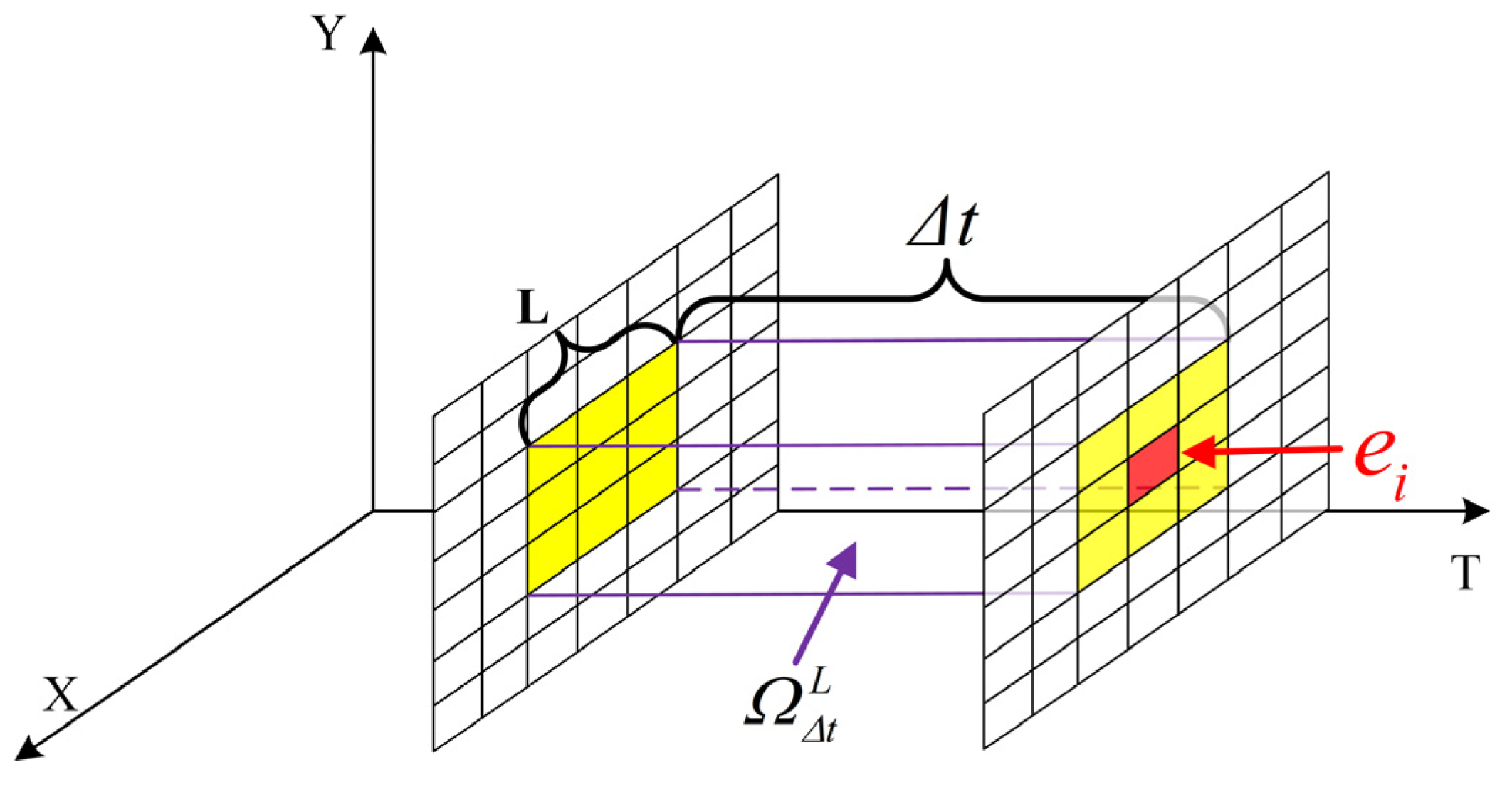
3.1. Spherical Spatio-Temporal Neighborhood

Among the existing event data denoising approaches, all employ the traditional cubic spatio-temporal neighborhood, as depicted in Figure 3.

This approach sets a cubic spatio-temporal neighborhood ${\Omega }_{\Delta t}^L$ for each event $e_i$ with an $L\times L$ spatial neighborhood as the base and an event duration $\Delta t$ as the height:

$${\Omega }_{\Delta t}^L\left(e_i\right)=\left\{e_j=({\mathit{u}}_j,t_j,p_j)\left|\left|{\mathit{u}}_j-{\mathit{u}}_i\right|<\Delta \mathit{u},t_j-t_i<\Delta t\right.\right\}.$$

(8)

However, to a certain extent, such processing methods separate the spatial and temporal information of events, losing the tightly coupled nature of some valid events regarding spatio-temporal information. Inspired by the spherical voxelization in the VRHCF point cloud processing method [34], we refined the traditional cubic spatio-temporal neighborhood and proposed a representation method based on the spherical spatio-temporal neighborhood to further enhance the tight coupling of spatio-temporal information in event data. Existing studies [35,36,37] have demonstrated that spherical neighborhoods are more suitable for processing unstructured 3D data. Replacing traditional cubic spatio-temporal neighborhoods with spherical counterparts offers several potential advantages, particularly when handling event data and performing nearest neighbor searches. Spherical neighborhoods can more effectively capture spatio-temporal relationships between events due to their inherent geometric continuity and smoothness, which better adapts to local variations in data distribution. This geometric continuity inherently reduces boundary artifacts during neighborhood partitioning compared to cubic divisions, where sharp boundaries may create imbalanced feature representations. Furthermore, event data in spatio-temporal representations typically manifest as unstructured 3D data, and spherical neighborhoods are fundamentally aligned with computing meaningful geometric features from such data. Consequently, spherical spatio-temporal neighborhoods exhibit superior performance over cubic counterparts in both feature representation and spatio-temporal relationship modeling.

To construct the spherical spatio-temporal neighborhood, in the original event set $E$, we traverse the event $e_i({\mathit{u}}_i,t_i,p_i)$, remove the event polarity, and at this point, the event is mathematically equivalent to a three-dimensional space point $e_i(x_i,y_i,t_i)$. Subsequently, for each $e_i$, a threshold $r$ is determined, and a KD tree is constructed in the original event set for radius-based nearest neighbor search. Then, the nearest neighbor events are aggregated to form the spherical spatio-temporal neighborhood $B\left(e_i\right)$.

This spatio-temporal neighborhood $B\left(e_i\right)$ is a subset of the original event set $E$ and can be expressed as follows:

$$B\left(e_i\right)≔E\cap B\left(e_i,r\right)=\left\{e_j\left|e_j\in RNN\left(E;e_i,r\right)\right.\right\},$$

(9)

where the $RNN$ operator represents the radius-based nearest neighbor search in $E$ centered at $e_i$ with radius $r$.

However, due to the non-uniformity of spatio-temporal data on the scale, the selection of the radius of the spherical spatio-temporal neighborhood is challenging in practical applications. In an extreme case, if objects in the scene move at an extremely slow speed, the characteristic of the event data is that its spatial scale is very small over a relatively long time scale. This leads to the inevitable dominance of time information when calculating the radius, resulting in the failure of the spatial constraint of the spherical spatio-temporal neighborhood. Therefore, we introduce a penalty coefficient ${Lt}^{-1}$ before the time during the radius-based nearest neighbor search:

$$r_{Lt}=\sqrt{(x_j-x_i{)}^2+(y_j-y_i{)}^2+\left({Lt}^{-1}\right(t_j-t_i){)}^2}.$$

(10)

Thus, the spherical spatio-temporal neighborhood $B\left(e_i\right)$ is modified as follows:

$$B_{Lt}\left(e_i\right)=\left\{e_j\left|e_j\in RNN(E;e_i,r_{Lt})\right.\right\};$$

(11)

the resulting spherical space–time neighborhood is shown in Figure 4:

3.2. Event Density and Curvature Noise Reduction

As described in Section 2.2, the denoising of event cameras, that is, how to distinguish whether an event is triggered by a moving object in the scene, is a crucial task for their practical usage and the completion of subsequent visual tasks. The majority of existing methods rely on the assumption that valid events and noise events have dissimilar spatio-temporal correlations, namely that the noise in the event stream is random and sparse, and is sufficiently separated from the valid events caused by object motion in space and time. However, this assumption may fail in certain circumstances. For instance, when the overall lighting conditions are unstable and the amount of noise is excessive and dense within its spatio-temporal neighborhood, the performance of noise in terms of spatio-temporal correlation may closely resemble that of valid events, interfering with the filter’s judgment of valid events; or when valid events are very sparse, the filter may mistakenly filter them out as noise. To overcome this issue, based on the spherical neighborhood, we propose an event camera denoising method that combines event density and the motion consistency of valid events. It can be inferred from the discussion on spatio-temporal correlation that if an event is caused by the real motion of an object, there will be other events consistent with the object’s motion within its spatio-temporal neighborhood. That is, within a reasonable spatio-temporal neighborhood, events caused by the object’s motion can theoretically form a coherent “motion surface”. A fundamental geometric attribute of the surface is its curvature, which describes the rate of rotation of the tangent direction of the surface with respect to the arc length and is precisely defined through differentiation. Its geometric significance lies in quantifying the degree of curvature of the object’s surface. Due to the consistency of motion of valid events, the surface formed in the spatio-temporal domain is also consistent. On this consistent surface, the curvatures of each event point should be similar. This consistency of curvature reflects the coherence and regularity of the object’s motion. In contrast, noise events are outside the surface, and their curvature characteristics are different from those of valid events. Figure 5 shows an example of this idea.

Figure 5 illustrates that the effective events are triggered by the actual motion of the object in space and time, they form a sufficiently smooth surface together with other events in their spatio-temporal domain, and these events have approximately the same curvature numerically. On the other hand, as shown in Figure 5, noise events usually cannot be classified or fitted into a consistent surface, and their curvatures differ significantly from those of valid events numerically. In our method, we first statistically analyze the event density in the spherical spatio-temporal neighborhood for initial denoising, and then further distinguish whether an event is a noise point by estimating its curvature based on the characteristics of the motion consistency of valid events.

Our algorithm first calculates the event density within the spherical spatio-temporal neighborhood. The event density is used to describe the sparsity of the event’s spatio-temporal neighborhood. For the current event $e_i(x_i,y_i,t_i)$, according to Section 3.1, its spherical spatio-temporal neighborhood is $B_{Lt}\left(e_i\right)$, and the number of events in the spherical spatio-temporal neighborhood centered at $e_i$ is calculated and referred to as the event density $\rho \left(e_i\right)$ of $e_i$:

$$\rho (e_i)={\sum }_1^{j}j,e_j\in B_{Lt}(e_i),$$

(12)

when the event density is greater than or equal to the set threshold ${\rho }_{TH}$, the subsequent curvature calculation and denoising processes are executed. The threshold for event density is set to determine whether an event is an outlier noise.

In the subsequent curvature filtering, we first define the curvature in the event data. During the estimation of the curvature of the event set, the concept of Gaussian curvature of the hypersurface is employed.

The Hessian matrix is first defined as an n × n symmetric matrix associated with a second-order differentiable multivariate function $f(x_1,\dots ,x_n)$. It is defined by the second-order partial derivatives of the function, where each element of the matrix represents the rate of change of these derivatives. Specifically, the Hessian matrix $H_f$ for a function $f(x_1,\dots ,x_n)$ is constructed as follows:

$$H_f=\left[\begin{array}{cccc}{\displaystyle \frac{{\partial }^{2}f}{\partial x_1^2}}& {\displaystyle \frac{{\partial }^{2}f}{\partial x_1\partial x_2}}& \cdots & {\displaystyle \frac{{\partial }^{2}f}{\partial x_1\partial x_n}}\\ {\displaystyle \frac{{\partial }^{2}f}{\partial x_2\partial x_1}}& {\displaystyle \frac{{\partial }^{2}f}{\partial x_2^2}}& \cdots & {\displaystyle \frac{{\partial }^{2}f}{\partial x_2\partial x_n}}\\ ⋮& ⋮& \ddots & ⋮\\ {\displaystyle \frac{{\partial }^{2}f}{\partial x_n\partial x_1}}& {\displaystyle \frac{{\partial }^{2}f}{\partial x_n\partial x_2}}& \cdots & {\displaystyle \frac{{\partial }^{2}f}{\partial x_n^2}}\end{array}\right],$$

(13)

where ${\displaystyle \frac{{\partial }^2\mathrm{f}}{\partial {\mathrm{x}}_{\mathrm{i}}\partial {\mathrm{x}}_{\mathrm{j}}}}$ is the second-order partial derivative of the multivariate function. There is the following theorem:

Theorem 1: 

Given that a hypersurface in $R^n$ can be represented by the explicit function $x_n=f(x_1,\dots ,x_{n-1})$ and ${{\displaystyle \frac{\partial f}{\partial x}}}_i=0$ when $1\le i\le n-1$, then its Gaussian curvature at the origin can be expressed by the determinant of the Hessian matrix $H_f={\displaystyle \frac{{\partial }^{2}f}{\partial x_i\partial x_j}}$.

For the event set $E$, where the events $\left\{e_0,\dots ,e_n\right\}$, are distributed around a hypersurface $S$ in the spatio-temporal domain, by using mathematical methods to project the event set onto this hypersurface, we define the local Gaussian curvature at the hypersurface coordinate $(x_i,y_i,t_i)$ as the curvature $c_i$ of the event $e_i$. The projection method utilizes the least squares method. The specific process is as follows: we establish a local coordinate system $(u,v,w)$ at the event $e_i$, translate the coordinate origin $O$ to $e_i$ using the translation transformation matrix $T$, and take $e_i$ as the origin $O^{\prime }$ of the local coordinate system.

$$T=\left[\begin{array}{cccc}1& 0& 0& 0\\ 0& 1& 0& 0\\ 0& 0& 1& 0\\ x_i& y_i& t_i& 1\end{array}\right].$$

(14)

Other events $e_j$ within its spatio-temporal neighborhood $B_{Lt}\left(e_i\right)$ are also translated:

$$e_j(u_j,v_j,w_j)=pro{j}_{R^3}\left(\right[x_j,y_j,t_j,1]\cdot T),$$

(15)

where the homogeneous coordinates of the event data are used to facilitate matrix operations, and the operator $pro{j}_{R^3}$ indicates that the homogeneous coordinates are projected back into three-dimensional space. Mathematically, this is as simple as removing the 1 that are filled in to keep the dimensions uniform and downscaling the result of the calculation.

The local shape of an arbitrary hypersurface in three-dimensional space can be approximately described by a quadratic surface equation, as follows:

$$S(u,v)=a{u}^2+b{v}^2+cuv+du+ev+f.$$

(16)

Suppose the neighborhood contains $k$ points, that is, $j\in [0,k]$. To solve the unknown coefficients, construct the observation vector $\mathit{S}$, the design matrix $\mathit{X}$, and the coefficient vector $\mathit{C}$:

$$\mathit{S}={\left[s_1,\dots ,s_k\right]}^T=\left[\begin{array}{cccccc}{u}_1^2& v_1^2& u_1{v}_1& u_1& v_1& 1\\ ⋮& ⋮& ⋮& ⋮& ⋮& ⋮\\ u_k^2& v_k^2& u_k{v}_k& u_k& v_k& 1\end{array}\right]{\left[a,b,c,d,e,f\right]}^T=\mathit{X}\cdot \mathit{C}.$$

(17)

where $\mathit{X}$ is a k × 6 matrix, where k is the number of points in the neighborhood. Each row represents an observation of a point and each column corresponds to a parameter in the model. $\mathit{C}$ is a column vector consisting of the parameters of the surface equations.

In order to minimize the sum of squared errors $SSE\left(\mathit{C}\right)={‖{\mathit{S}}^{\prime }-\mathit{X}\cdot \mathit{C}‖}^2$ between the actual observations ${\mathit{S}}^{\prime }$ and the model predictions $\mathit{X}\cdot \mathit{C}$, the normal equation ${\mathit{X}}^T\mathit{X}\mathit{C}={\mathit{X}}^T{\mathit{S}}^{\prime }$ is obtained by taking its derivative with respect to $\mathit{C}$ and setting the derivative to zero, $\partial SSE\left(\mathit{C}\right)/\partial \mathit{C}=0$, from which the vector of coefficients is solved:

$$\mathit{C}=({\mathit{X}}^T\mathit{X}{)}^{-1}{\mathit{X}}^T{\mathit{S}}^{\prime }.$$

(18)

Once the optimal solution vector C is obtained, then all the parameters in the corresponding Equation (16) are known, by Theorem 1 and the definition, the curvature $c_i$ of the event $e_i$ at the origin $O^{\prime }\left(e_i\right)$ can be computed from the determinant of the Hessian matrix $H_S$ of the hypersurface equation:

$$c_i=\mathit{det}(H_S)=\mathit{det}\left[\begin{array}{cc}{\displaystyle \frac{{\partial }^{2}S}{\partial u^2}}& {\displaystyle \frac{{\partial }^{2}S}{\partial u\partial v}}\\ {\displaystyle \frac{{\partial }^{2}S}{\partial v\partial u}}& {\displaystyle \frac{{\partial }^{2}S}{\partial v^2}}\end{array}\right].$$

(19)

An alternative calculation of the Gaussian curvature of a surface is as follows, starting with the parameterization of the surface by Equation (16):

$$K(p,q)=\left(u\right(p,q),v(p,q),w(p,q\left)\right)$$

(20)

where $K$ denotes the parameterized surface, $p, q$ are parameters, and $u, v, w$ are the 3D coordinates of the fitted surface. Subsequently, the first-order partial derivatives and second-order partial derivatives of the parameterized surface are calculated as follows:

$$K_p={\displaystyle \frac{\partial K}{\partial p}}, K_q={\displaystyle \frac{\partial K}{\partial q}}.$$

(21)

$$K_{uupp}={\displaystyle \frac{{\partial }^{2}K}{\partial p^2}}, K_{pq}={\displaystyle \frac{{\partial }^{2}K}{\partial p\partial q}}, K_{qq}={\displaystyle \frac{{\partial }^{2}K}{\partial q^2}}.$$

(22)

The unit normal vector $\mathit{N}$ can be obtained by the fork product of the first-order partial derivatives and normalized:

$$\mathcal{N}={\displaystyle \frac{K_p\times K_q}{\left.∥K_p\times K_q\right|}}.$$

(23)

Finally, the first fundamental quantities $E, F, G$ and the second fundamental quantities $L, M, N$ of the parameterized surface are calculated as follows:

$$\left\{\begin{array}{c}E=K_p·K_p,F=K_p·K_q,G=K_q·K_q\\ L=K_{pp}·N,M=K_{pq}·N,N=K_{qq}·N\end{array}\right..$$

(24)

The final Gaussian curvature $\mathcal{K}$ is defined as follows:

$$\mathcal{K}={\displaystyle \frac{LN-M^2}{EG-F^2}}.$$

(25)

According to Equation (18), the Hessian matrix method estimates the local curvature of the surface through the second-order partial derivatives of the function, but this method is more sensitive to the computational error of the Hessian matrix, and the error of the first-order partial derivatives will directly affect the computation of the second-order partial derivatives, resulting in the accumulation of the error, which makes the curvature estimation become unstable. According to Equation (25), the parametric surface method requires an explicit parametric representation of the surface to compute the Gaussian curvature through the first and second fundamental quantities, and this method is more sensitive to the parameterization error, especially in the sharp edges or high curvature regions of the surface, where small parameterization changes may lead to significant changes in the curvature. It can be seen that the parametric surface method requires further parameterization of the surface and performs poorly at the edges of the surface, so we use the Hessian matrix method to estimate the Gaussian curvature directly, which is more able to satisfy the requirements of the event curvature calculation process.

After traversing and obtaining the curvature $c_i$ of each event in the event set, the curvature values are expected to be consistent overall due to the curvature consistency of the “motion surface” caused by the consistency of the true event motion. This implies that the local geometry of the “motion surface” is flat, i.e., the Gaussian curvature is close. Therefore, a percentage threshold is set to select events that represent a fixed proportion of the total events and have Gaussian curvature values close. This approach allows for the statistical definition of a set of events whose local geometric properties exhibit flatness, that is to say, Gaussian curvature approximates. By adjusting this percentage threshold, the method can be adapted to different noise levels, ensuring that the filtered event set maintains consistent geometric properties.

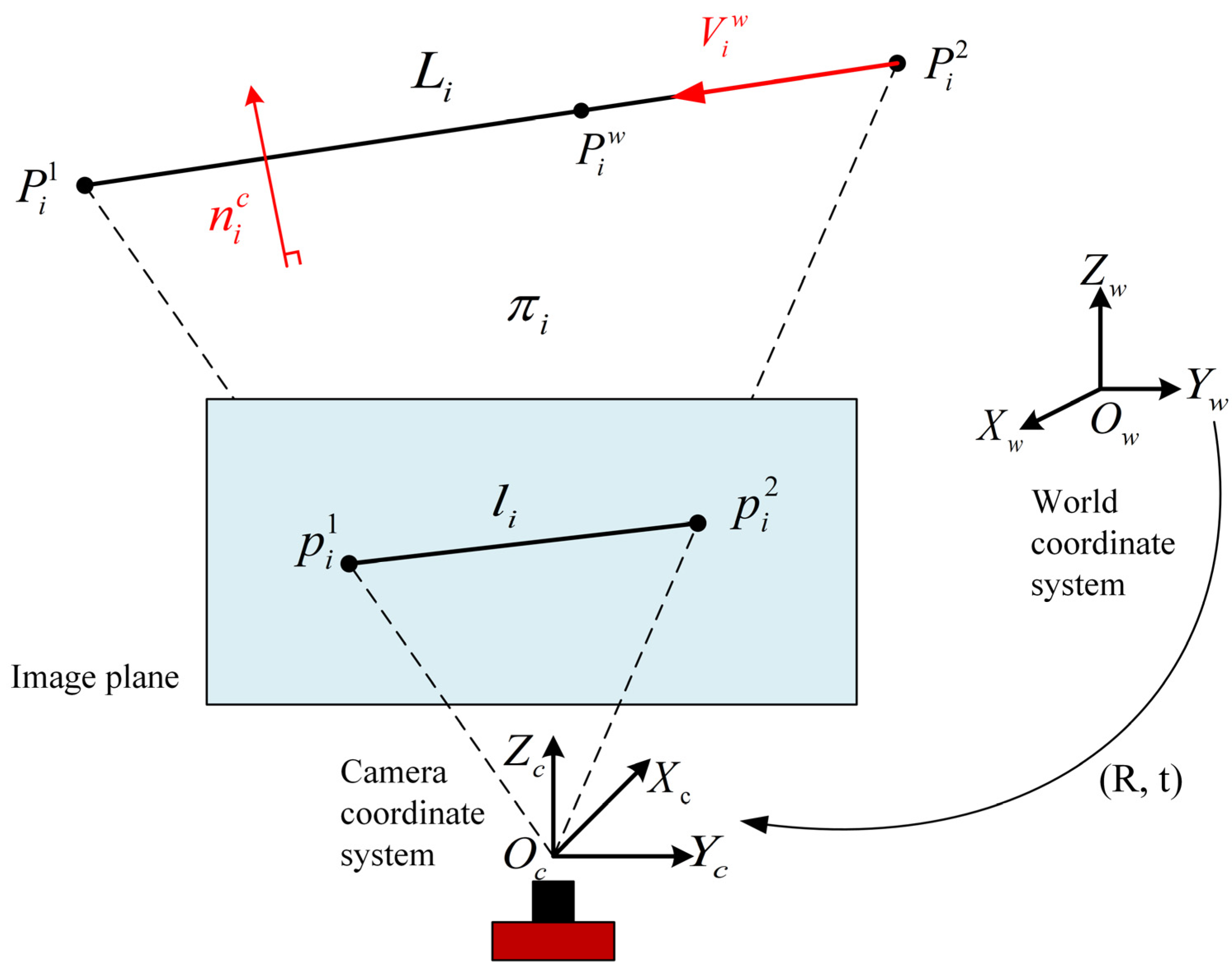
3.3. Noise-Reduced Event-Based Pose Estimation Framework

In this section, a framework for object pose estimation using an event camera is constructed to evaluate the performance improvements attributed to the noise reduction approach within the context of event-based object pose estimation utilizing line features. This framework is tightly integrated by combining the noise reduction algorithm with the OPnL algorithm [38] and the ELOPET method [33] proposed by Liu et al. The noise reduction algorithm is applied to the event stream to effectively mitigate the impact of noise and outliers, ensuring that subsequent pose estimation processes are conducted on a cleansed event stream. The noise-reduced event images are then utilized to obtain the 2D line feature parameters of the object required by the OPnL algorithm for initial pose estimation.

The noise suppression algorithm plays a pivotal role in the initial phase of the framework, which is directly applied to the event stream generated by the event camera. This preprocessing step is crucial as it significantly reduces the effect of noise and outliers present in the raw event data. After noise reduction, the 2D line feature parameters of the target are extracted using the noise-reduced event image. These parameters are essential for the OPnL algorithm because the OPnL algorithm requires accurate feature data to initiate the pose estimation and compute the initial estimate of the target pose. The noise-canceled event stream and the initial pose estimated by the OPNL algorithm are the basis of the ELOPET method, which further refines the pose estimation by tracking these line features in the event stream. The combination of the noise reduction algorithm with the OPnL and ELOPET methods is not only sequential but also synergistic. The noise suppression algorithm prepares the data by improving the quality of the data, which is essential for the OPnL algorithm to accurately identify and utilize the 2D line features for the initial pose estimation. Once the initial pose is estimated, the ELOPET method builds on this estimate, utilizing the noise-reduced event stream to track the line features and iteratively improve the pose estimate.

The common PNL problem is shown in Figure 6, which can be simply expressed as a method of calculating the camera’s rotation matrix $R$ and translation vector $t$ in space from a single view using n sets of (n ≥ 4) 2D/3D line correspondents.

$L_i$ is a three-dimensional line feature defined by the normalized direction vector ${\mathit{v}}_{\mathit{i}}^{\mathit{w}}$ and the random point $P_{\mathit{i}}^w$ on it, and its corresponding two-dimensional projection is determined by the point pairs $(p_i^1,p_i^2)$. The projection plane ${\pi }_i$ is determined by the three-dimensional line feature $L_i$ and the camera’s optical center $O_c$, and its normal vector is $n_i^c$. From the mathematical fact that $n_i^c$ and ${\pi }_i$ are perpendicular to each other, the measurement equation of the PNL problem can be obtained as follows:

$$\left\{\begin{array}{c}(n_i^c{)}^{T}R{\mathit{v}}_i^w=0\\ \left(n_i^c{)}^T\right(R{P}_{\mathit{i}}^{\mathit{w}}+t)=0\end{array}\right.,$$

(26)

where $n_i^c={[x_i,y_i,z_i]}^T$, ${\mathit{v}}_i^w={[X_{vi},Y_{vi},Z_{vi}]}^T$, and $P_i^w={[X_{Pi},Y_{Pi},Z_{Pi}]}^T$.

In the OPNL method, the rotation matrix $R$ is first represented by the unit quaternion $q$, $q={[q_0,q_1,q_2,,q_3]}^T$ and satisfies $‖q=1‖$:

$$\left.R=\left[\begin{array}{ccc}{q}_0^2+q_1^2-q_2^2-q_3^2& 2(q_1{q}_2-q_0{q}_3)& 2(q_1{q}_3+q_0{q}_2)\\ 2(q_1{q}_2+q_0{q}_3)& q_0^2-q_1^2+q_2^2-q_3^2& 2(q_2{q}_3-q_0{q}_1)\\ 2(q_1{q}_3-q_0{q}_2)& 2(q_2{q}_3+q_0{q}_1)& q_0^2-q_1^2-q_2^2+q_3^2\end{array}\right.\right].$$

(27)

It is then parameterized Cayley–Gibbs–Rodriguez (CGR):

$$\left.R={\displaystyle \frac{1}{H}}\left[\begin{array}{ccc}{1+q}_1^2-q_2^2-q_3^2& 2q_1{q}_2-2q_3& 2q_1{q}_3+2q_2\\ 2q_1{q}_2+2q_3& 1-q_1^2+q_2^2-q_3^2& 2q_2{q}_3-2q_1\\ 2q_1{q}_3-2q_2& 2q_2{q}_3+2q_1& 1-q_1^2-q_2^2+q_3^2\end{array}\right.\right]={\displaystyle \frac{1}{H}}M,$$

(28)

where $H={1+q}_1^2+q_2^2+q_3^2$.

Combining Equations (26) and (28), the unconstrained minimized equations are constructed and the following is obtained:

$$\left\{\begin{array}{c}(n_i^c{)}^{T}M{\mathit{v}}_i^w=0\\ \left(n_i^c{)}^T\right(M{P}_i+Ht)=0\end{array}\right..$$

(29)

Let $s={[1 ,q_1 ,q_2 ,q_3 , q_1^2 ,q_1{q}_2 ,q_1{q}_3 ,q_2^2 ,q_2 ,q_3 , q_3^2]}^T$, then Equation (21) yields:

$$Q_i^{T}s=\left[\begin{array}{ccc}0& 0& 0\\ {-x}_i& -y_i& -z_i\end{array}\right]Ht=N_{i}Ht,$$

(30)

where $Q_i$ is a 10 × 2 matrix obtained by linearly combining the elements of $n_i^c$, ${\mathit{v}}_i^w$, and ${\mathit{P}}_{\mathit{i}}^{\mathit{w}}$.

There are generally $n$ lines in the PNL problem, that is, when $i=0,1,2,\cdots n$, then Equation (29) can be further derived as follows:

$$\left[\begin{array}{c}{Q}_1^T\\ Q_2^T\\ ⋮\\ Q_n^T\end{array}\right]s=\left[\begin{array}{c}{N}_1\\ N_2\\ ⋮\\ N_n\end{array}\right]Ht\iff Qs=NHt.$$

(31)

If $s$ is known, then $Ht$ can be solved using the Moore–Penrose matrix inverse as follows:

$$Ht={\left(N^{T}N\right)}^{-1}{N}^{T}Qs=N^{+}Qs.$$

(32)

By substituting $Ht$ in Equation (30) with Equation (32), the following equation is obtained:

$$Q_i^{T}s=N_i{N}^{+}Qs.$$

(33)

Because of noise, Equation (33) is not always exactly equal, and the residual is defined as follows:

$${\eta }_i=(Q_i^T-N_i{N}^{+}Q)s=E_{i}s,$$

(34)

thus, the least square cost function of the PNL problem is obtained:

$$\epsilon ={\sum }_{i=1}^n{\eta }_i^2=s^T\left({\sum }_{i=1}^n{E_i }^T{E}_i\right)s=s^{T}Gs.$$

(35)

The first-order optimality condition of the cost function is as follows:

$${\displaystyle \frac{\partial \epsilon }{\partial q_1}}=0 , {\displaystyle \frac{\partial \epsilon }{\partial q_2}}=0 , {\displaystyle \frac{\partial \epsilon }{\partial q_3}}=0.$$

(36)

Finally, the Gröbne basis technique is used to solve the multivariate polynomial equation constructed from Equation (11), and the initial rotation $R$ and translation vectors $t$ can be obtained by substituting the result $s$ back to Equations (28) and (32).

The ELOPET method is utilized for pose optimization and tracking after obtaining the initial pose. This method first establishes the correspondence between 2D event frame and 3D model lines through event–line matching. Specifically, 3D line features are projected onto the 2D image via the initial pose. As shown in Figure 6, points $P_{\mathit{i}}^1$ and $P_{\mathit{i}}^2$ on the 3D line feature $L_i$, are selected, and their 2D projections are the endpoints $(p_{\mathit{i}}^1,p_{\mathit{i}}^2)$ of $l_i$. The $l_i$ can be defined by the homogeneous coordinates of $p_{\mathit{i}}^1$ and $p_{\mathit{i}}^2$:

$$l_i={\displaystyle \frac{p_i^1\times p_i^2}{\left|p_i^1\times p_i^2\right|}}={\left[l_{ix},l_{iy},l_{iz}\right]}^T.$$

(37)

Based on the correspondence between 2D and 3D line features, the event–line distance between the event $e_j$ and the projected line $l_i$ can be obtained:

$$d_{ij}={\displaystyle \frac{e_j^T{l}_i}{\sqrt{l_{ix}^2+l_{iy}^2}}}.$$

(38)

Events are screened according to the event–line distance to ensure that each event $e_j$ corresponds to a unique 2D line feature $l_i$. The line feature tracking and pose optimization are performed using a pose-tracking method that minimizes the event–line distance while assigning different weights ${\omega }_{ij}$ to each event. Let the pose parameters $X=\{R,t\}$, the optimal pose parameter estimate $X^{*}$ is obtained by solving the following optimization problem:

$$X^{*}=\underset{X}{\mathit{arg\; min}}C\left(X\right)=\underset{X}{\mathit{arg\; min}}{\sum }_{i,j}\rho \left(d_{ij}/{\widehat{\sigma }}_{\alpha }\right)=\underset{X}{\mathit{arg\; min}}{\sum }_{i,j}\rho \left(u_{ij}\right),$$

(39)

where $\alpha$ represents different estimation methods, the scale estimator ${\widehat{\sigma }}_S$ is as follows:

$${\widehat{\sigma }}_S=\sqrt{{\displaystyle \frac{1}{0.199mn}}{\sum }_{j=1}^m{\sum }_{i=1}^n{\omega }_{ij}\cdot d_{ij}^2},$$

(40)

${\widehat{\sigma }}_{MM}$ is the standard deviation obtained from the residual of S estimation. $\rho (·)$ is the robust cost function, Tukey’s bisquare objective function is as follows:

$$\rho \left(u_{ij}\right)=\left\{\begin{array}{cc}{\displaystyle \frac{u_{ij}^2}{2}}-{\displaystyle \frac{u_{ij}^4}{2c^2}}+{\displaystyle \frac{u_{ij}^6}{6c^4}}& ,\left|u_{ij}\right|\le c\\ {\displaystyle \frac{c^2}{6}}& ,\left|u_{ij}\right|>c\end{array}\right.,$$

(41)

where $c$ is a finite constant. Further minimization is converted into finding the stationary points of the function:

$${\sum }_{i,j}\rho \left(u_{ij}\right){\displaystyle \frac{\partial \rho }{\partial \left(u_{ij}\right)}}=0.$$

(42)

The influence curve and weight function are also defined:

$$\psi \left(u_{ij}\right)={\rho }^{\prime }\left(u_{ij}\right)\triangleq {\displaystyle \frac{\partial \rho }{\partial \left(u_{ij}\right)}}=\left\{\begin{array}{cc}{u}_{ij}{\left[1-{\left({\displaystyle \frac{u_{ij}}{c}}\right)}^2\right]}^2\hfill & ,\left|u_{ij}\right|\le c\hfill \\ 0\hfill & ,\left|u_{ij}\right|>c\end{array}\right.,$$

(43)

$${\omega }_{ij}\triangleq {\displaystyle \frac{\psi \left(u_{ij}\right)}{u_{ij}}}=\left\{\begin{array}{cc}{\left[1-{\left({\displaystyle \frac{u_{ij}}{c}}\right)}^2\right]}^2\hfill & ,\left|u_{ij}\right|\le c\\ 0\hfill & ,\left|u_{ij}\right|>c\end{array}\right..$$

(44)

The initial estimation parameters are obtained using S estimation, where the threshold $c=1.547$ in Equation (42). The obtained initial estimation parameters are iteratively optimized using MM estimation, where the threshold $c=4.685$ in Equation (42). After updating the weight ${\omega }_{ij}$ according to Equation (43), calculate the gradient of the residual function until it is less than the set threshold:

$$‖\nabla C\left(X\right)‖<Threshold.$$

(45)

The $X$ satisfying Equation (45) is the optimal pose estimation parameter $X^{*}$. The specific process of the overall framework is shown in Figure 7.

4. Results

In this section, we evaluate the noise reduction algorithms using simulated purely noisy data and data collected by an event camera in the real world, respectively. The event camera noise reduction method proposed in this paper is compared with three filtering methods: BAF (background activity filter) [8], KNoise [11], and YNoise [12].

The setting of filter parameters is crucial, and manual tuning of parameters is indispensable. To ensure a fair comparison, the parameter selection referred to those employed in the original literature [8,11,12] and was subsequently fine-tuned based on practical experience with event cameras, with the parameters ultimately chosen as follows: BAF, with a maximum time difference in microseconds for events to be considered correlated and not filtered out, set at 2000 μs. KNoise, with the time interval to look up the spatio-temporal neighbors (deltaT) at 1000 μs and the number of supporting pixels (supporters) at 1. YNoise, with a spatio-temporal neighborhood time window of 10,000 μs, an L × L density matrix with L set to 3, and a density threshold of 1. The algorithm parameters in this paper are set as follows: the density threshold is set to 5, and the spatio-temporal neighborhood radius is set to 2. As described in Section 3.1, the scale inhomogeneity of spatio-temporal data can cause the failure of spatial constraints, which in turn affects the formation of spherical spatio-temporal neighborhoods, while the event camera time resolution is usually at the microsecond level, the length of the event frame is usually 30,000 microseconds in the usual use scenarios; this time length can adapt to most of the motion intensities in most of the scenarios. In order to match the spatial scale with a resolution of (360, 246) used in this experiment, it is necessary to multiply by a penalty coefficient capable of shrinking the temporal values to the same scale. In practice, we found that $Lt={10}^4$ can satisfy the noise reduction needs in most scenes, and for a fair comparison with other algorithms, we fixed this value in all scenes. And the curvature percentage threshold is set to 80%.

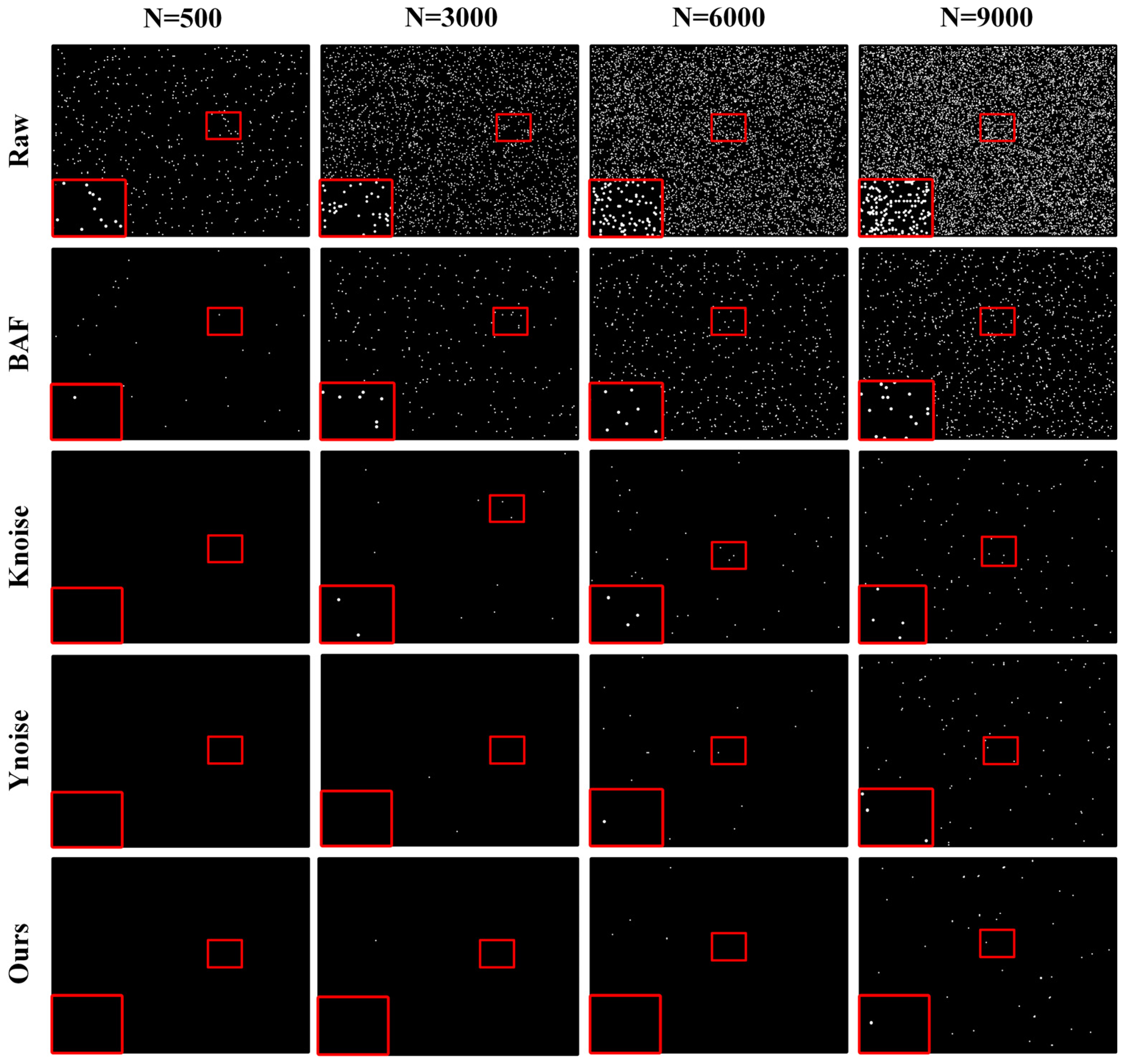
4.1. Pure Noise Event Flow Noise Reduction

In the evaluation of denoising algorithms, different metrics are employed for distinct categories of noisy data. Specifically, the noise reduction ratio (NRR) is used to assess the performance of denoising algorithms applied to simulated data. The NRR is a direct denoising metric, defined as the ratio of the number of events filtered out to the total number of original events before filtering:

$$NRR={\displaystyle \frac{E_{noise}^{fo}}{E_{noise}^o}},$$

(46)

where $E_{noise}^{fo}$ denotes the number of events filtered out and $E_{noise}^o$ denotes the total number of original events before filtering. The simpler pure noise reduction experiment is first set up, in which simulation-generated pure noise event stream data are used. The event camera pixels operate independently, and under normal conditions, each pixel does not interfere with the other, i.e., the probability of generating BA noise at a pixel at a certain moment is equal and follows a uniform distribution. It is known from Section 2.2 that the mathematical model of BA noise of the event camera conforms to the Poisson distribution, and its level is determined by the parameter λ of the Poisson distribution. The simulation approach is therefore to determine the total number of noises based on the noise level, generate uniformly distributed random events in pixel space, and subsequently generate noise stream data close to that in the real world by adding incremental timestamps to these events. Four sets of purely noisy event stream data with different noise levels are generated, each with a spatial resolution of 346 × 260 and a time length of 30 ms, which is the time length of an event frame in most event data representation methods. The noise level is set based on the following calculation: in the ideal case, when the BA noise is dominated by leakage noise, the noise generation rate is about 0.1 Hz, resulting in a total noise count of approximately 269 events for a 30-millisecond frame. In the low-light environment, the BA noise is dominated by scattering noise, and the noise generation rate increases, reaching around 5 Hz, leading to a total noise count of approximately 13,494 events. Therefore, the total number of noise events in the four groups is set to be 500, 3000, 6000, and 9000, respectively, which can represent the gradual increase of the BA noise level of the event camera from the ideal situation to the extreme situation. The first row in Figure 8 visualizes purely noisy event frames at different noise levels, respectively. It can be seen that at extremely low illumination, the ratio of BA noise is large and causes very serious interference with the imaging of the event camera.

Subsequently, various noise reduction algorithms were applied to process the simulated pure noise event stream data. To quantitatively evaluate the performance of various filtering algorithms, the noise reduction ratio (NRR) was utilized to analyze the performance of different methods. The experimental results and the performance of each algorithm are presented in

Table 1. Experimental results of noise reduction for purely noisy event streams.

Noise level	BAF		KNoise		YNoise		Ours
	Residual Noise	NRR	Residual Noise	NRR	Residual Noise	NRR	Residual Noise	NRR
500	34	93.20%	0	100%	0	100%	0	100%
3000	246	91.80%	13	99.57%	3	99.90%	2	99.93%
6000	581	90.32%	42	99.30%	16	99.73%	6	99.90%
9000	1077	88.03%	106	98.82%	89	99.01%	67	99.26%

, where the first column displays the total number of noise events, and the remaining columns show the number of residual noise events after applying different methods, along with the corresponding noise reduction ratios.

As demonstrated in the tabular data, at a noise level of N = 500, all the algorithms exhibit high NRR. Notably, KNoise, YNoise, and our algorithm all attain 100%, which is attributable to the fact that the spatio-temporal correlation between the noises at this time is found to be very weak, and the spatio-temporal filtering algorithms are all capable of accurately identifying the noises. However, as the noise level increases, the performance of the BAF algorithm exhibits a substantial decline, accompanied by an increase in residual noise. Concurrently, the remaining algorithms begin to manifest residual noise, though their denoising rate indicators remain less impacted, with all maintaining a rate above 98%. However, at the maximum noise level of N = 9000, the BAF algorithm has completely failed. At this time, the residual noise events have reached 1077, and the NRR is only 88.03%, compared to the performance of KNoise and YNoise, which has also declined, with NRRs 98.82% and 99.01%, respectively. However, the Ours algorithm demonstrates notable efficacy, with an NRR of 99.26% and a mere 67 residual noise events, indicating its effectiveness even under conditions of extreme noise. A visual representation of the noise reduction results is provided in Figure 8.

It can be observed that for relatively clean leakage noise (N = 500), all algorithms perform well, being able to completely filter out pure noise. As the noise level increases, the standard spatio-temporal filter BAF begins to fail, unable to accurately identify noise, which is predictable given that this method only performs simple density statistics on the event stream. When the experimental conditions reach low-light scenarios (N = 6000), Knoise also begins to exhibit missed detection of noise. Under extreme conditions (N = 9000), the noise generation rate is close to the generation rate of valid events, and we can see that the white noise is densely distributed in all pixels of the event frames, and the event camera may not work properly at this time. The white noise is uniformly distributed in the denoised event frames of KNoise and BAF, which indicates that the two algorithms are completely ineffective in achieving the filtration of the pure noise. At this point, although both YNoise and our algorithms maintain good noise reduction rates, stubborn noise has begun to appear in the denoised image, which may still interfere with the normal operation of the event camera. This is an important factor that limits event cameras to practical industrial production. At the same time, it was observed that the minimal residual noise not filtered out by the noise reduction algorithm presented in this paper, at a noise level of N = 9000, is more compact and dense in the denoised images compared to those resulting from the YNoise algorithm. This increased compactness and density indicate a stronger spatio-temporal correlation, which is a notable advantage of the spherical spatio-temporal neighborhood used in our approach—its enhanced sensitivity to dense events. This characteristic contributes to the improved performance of our algorithm in noise reduction.

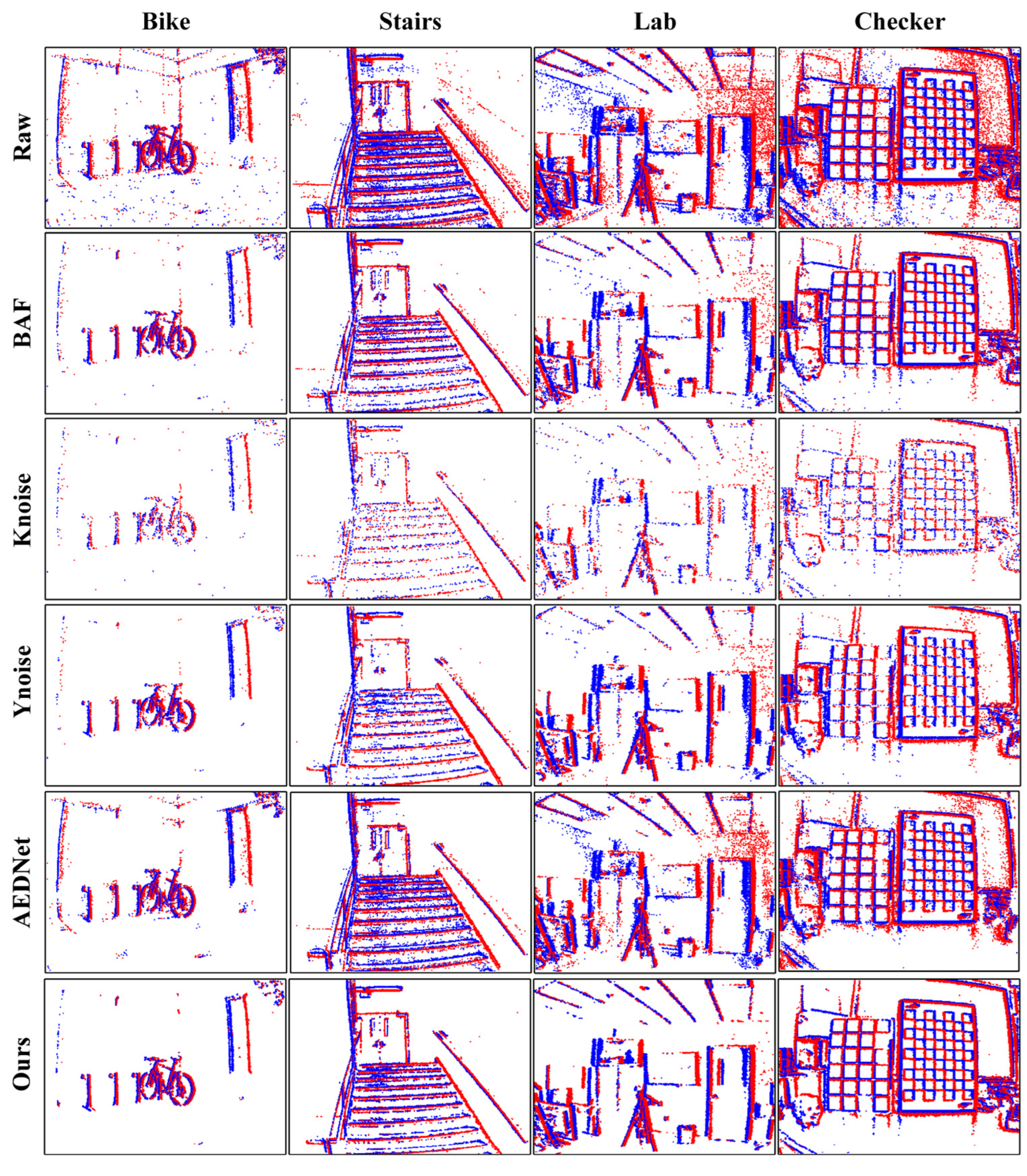
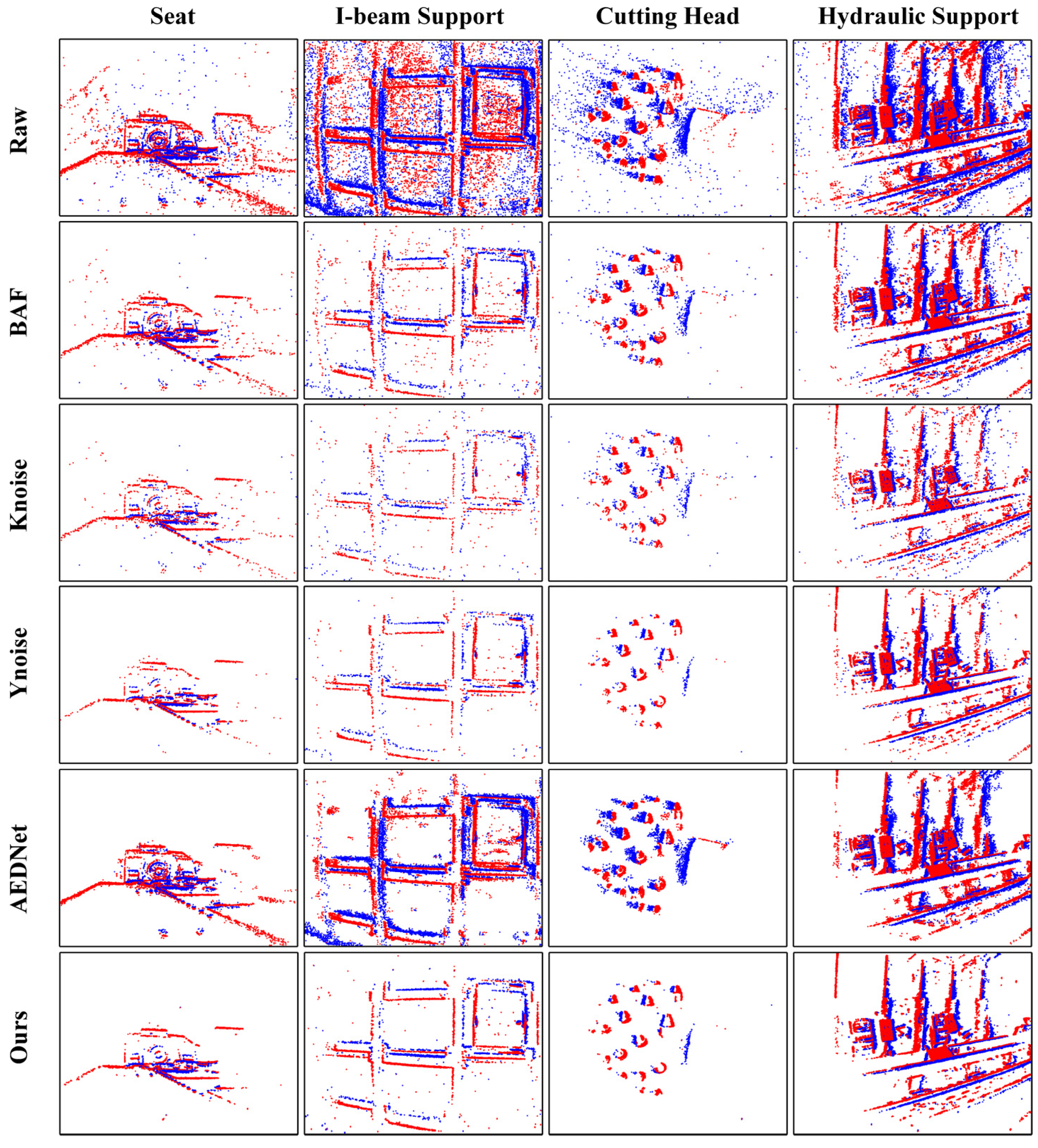
4.2. Event Data in Real-World Experimentation

As discussed in Section 2.2, event cameras are highly susceptible to noise. In practice, although some obvious outliers can be accurately identified as noise, other randomly distributed noise may be intermingled with valid events, making it challenging to obtain a ground truth image in the context of event camera applications. Consequently, numerous metrics have been proposed to evaluate the denoising effects on real event data, each with its specific application scenarios. The event structural ratio (ESR) is a novel non-reference metric for event denoising, which is independent of both the number of events and their projection directions. Instead, it is an intrinsic property of the events themselves. The literature [12] demonstrates that ESR exhibits a negative correlation with noise levels, as evidenced by rigorous mathematical derivations and empirical experiments. Additionally, the ESR is computationally efficient and does not rely on active pixel sensor information or manual labeling. Therefore, this paper selects the ESR as the evaluation metric for denoising algorithms applied to real-world data. To further validate the superiority of our proposed noise reduction algorithm, we also compared it with the deep learning-based noise reduction algorithm, AEDNet, in experiments with real-world collected event data. The deep learning experiments were conducted using the Windows 10 operating system, PyTorch11.3 deep learning development framework, and Python3.8 as the development language. The CPU used in the experiments is Intel Core i7-8750H and the GPU is NVIDlA GeForce GTX 1070. The batchsize is set to 8, the initial learning rate is set to 0.001, and the epoch is 50.

4.2.1. DVSNoise20 Dataset Experimentation

Noise reduction experiments were conducted on the DVSNoise20 dataset. This dataset, constructed by R. Wes Baldwin et al., utilizes a DAVIS346 event camera with a resolution of 346 × 260 and comprises 48 event sequences across 16 fixed scenes. It provides comprehensive data including traditional intensity images, event streams, IMU data, and ground truth labels representing the probability of event generation. These data are primarily used to evaluate the performance of event-denoising algorithms based on real sensor data. In this experiment, four sequences with varying levels of complexity and speed were selected: bike and labFast represent complex texture scenes, while stairs and checkerSlow represent regular textures; In addition, labFast is characterized by high-speed motion, whereas bike, stairs, and checkerSlow exhibit low-speed motion.

The proposed algorithm was compared against algorithms BAF, KNoise, and YNoise using the aforementioned sequences.

Table 2. ESR results of different denoising methods on the DVSNoise20 dataset. The bold numbers are the highest ESR values, signifying the best noise reduction performance.

	Bike	Stairs	LabFast	CheckerSlow
Raw	1.912	1.395	1.313	1.147
BAF	0.799	0.829	0. 961	1.068
KNoise	0.568	0.532	0.688	0.594
YNoise	0.796	0.790	0.917	1.128
AEDNet	0.809	0.830	1.130	1.197
Ours	1.898	1.392	1.286	1.289

presents the ESR (event signal-to-noise ratio) indicators for different algorithms on the DVSNoise20 dataset, where the bold numbers are the highest ESR values, signifying the best noise reduction performance.

As indicated in Table 2, BAF and YNoise demonstrate superior performance compared to KNoise under various textures and motion velocities. The proposed algorithm in this paper achieves the highest ESR across all four sequences, thereby indicating the best noise reduction effect. Specifically, our algorithm outperformed BAF by 60.38%, KNoise by 146.22%, YNoise by 61.53%, and AEDNet by 47.48% in terms of average ESR assessment. It is also observed that, compared to the original data, the ESR values of the other three non-deep learning algorithms decrease after denoising: BAF experiences an average reduction of 33.15%, KNoise of 57.02%, and YNoise of 33.40%. The AEDNet algorithm does not have a high ESR score in the first two scenarios, but the ESR degradation is not very severe in the last two scenarios. In contrast, the ESR of event data processed by the algorithm in this paper only decreased by 1.01% in the first three sequences compared with the original data, and increased by 3% in the checkerSlow sequence. This outcome is anticipated, as the visualization results in Figure 9 reveal that the noise level in the current frames of these sequences is not particularly high. Under such conditions, the algorithm inevitably misclassifies some valid events as noise, thereby disrupting the event structure ratio of the original event data and leading to a decrease in the ESR metric. The proposed algorithm enhances the correlation of spatio-temporal information in event data by employing a spherical spatio-temporal neighborhood; on this basis, it integrates filtering based on event density and event curvature, thereby achieving higher recognition capabilities for spatio-temporal dense and continuous effective events. This approach enables the algorithm to accurately identify and filter out noise while retaining as many valid events as possible, thereby significantly improving the performance of the event-filtering algorithm.

Figure 9 provides a qualitative comparison of the noise reduction effects of different algorithms on the four sequences.

While optimizing for memory efficiency, KNoise results in poor filtering performance, primarily characterized by a severe loss of valid events. Although BAF retains a sufficient number of valid events, it also preserves more noise. In contrast, YNoise and the proposed algorithm achieve a better balance in this regard. Whereas AEDNet performs well visually in simple scenes, retaining valid events while trying to remove most of the noise, it appears to retain a lot of noise in the lab scene and checker scene, which may be related to the training dataset, where the training dataset of the original AEDNet algorithm is for event imaging of single objects, which is likely to lead to its different scene differences in performance. In terms of image details, the proposed algorithm demonstrates superior performance on the stairs sequence, presenting clearer lines of the staircase. On the labFast and checkerSlow sequences, the filtering results of the proposed algorithm not only remove more noise but also render the ceiling patterns and the lines of the calibration board more distinct.

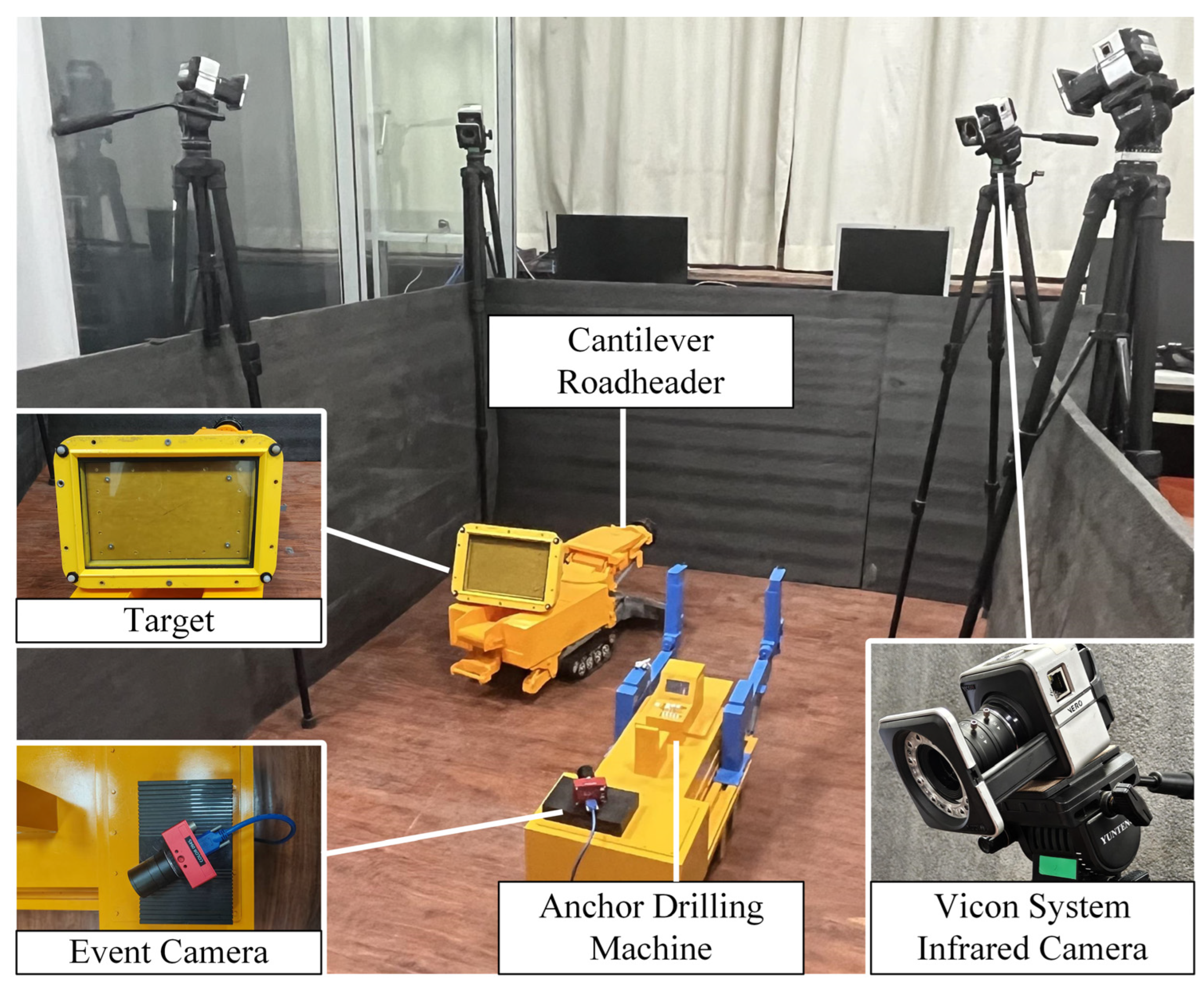
4.2.2. Underground Coal Mine Laboratory Experimentation

To further ascertain the robustness of the proposed algorithm, additional tests were conducted using independently collected event camera data. Event camera DAVIS346 (346 × 260) was used to collect data in the simulated coal mine underground environment laboratory at Xi’an University of Science and Technology (XUST), which is characterized by poor lighting and complex textures. Data were gathered across three distinct scenarios: the fully mechanized face, the digging face, and the return tunnel. The fully mechanized face was characterized by the most complex textures, the digging face predominantly featured the event camera’s imaging of machinery and equipment in a dimly lit setting, and the return tunnel exhibited the most adverse lighting conditions. The experimental setup is illustrated in Figure 10.

Four distinct noise reduction algorithms were employed in the experiment to process four representative datasets (namely, the driving seat of the roadheader, the I-beam support, the cutting head of the roadheader, and the hydraulic support). The event structural ratio (ESR) metrics for these algorithms on the simulated coal mine laboratory data are presented in

Table 3. ESR results for different denoising methods on the coal mine laboratory data. The bold numbers are the highest ESR values, signifying the best noise reduction performance.

	Seat	I-Beam Support	Cutting Head	Hydraulic Support
Raw	0.697	0.665	1.114	0.752
BAF	0.729	0.732	1.088	0.608
KNoise	0.520	0.589	0.887	0.586
YNoise	0.783	0.722	1.037	0.660
AEDNet	0.709	0.663	1.075	1.027
Ours	0.772	0.762	1.126	1.045

, with the bolded figures indicating the superior noise reduction performance associated with the highest ESR values.

As depicted in Table 3, the KNoise algorithm exhibits the least favorable performance under challenging conditions, such as low-light environments and scenarios with intricate textures. This underperformance is attributed to the algorithm’s memory optimization strategy, which, while beneficial for reducing memory usage, adversely affects its ability to handle complex data. In contrast, our proposed algorithm demonstrates superior performance across three tested scenarios, achieving the highest overall ESR scores. Specifically, our algorithm outperforms the BAF algorithm by an average margin of 17.36%, surpasses the KNoise algorithm by 43.49%, betters the YNoise algorithm by 15.71%, and higher than the AEDNet by 5.76% in terms of average ESR evaluation. Notably, our algorithm’s advantage is particularly pronounced in sequences handling hydraulic support, which are characterized by their complex textures and where our algorithm achieves significantly higher ESR values compared to its counterparts.

Figure 11 presents a qualitative comparison of noise reduction outcomes.

Consistent with our previous experimental findings, KNoise achieves moderate success in less complex scenarios, such as those involving seats and cutting heads. However, its performance deteriorates in more structurally complex scenarios, like those involving hydraulic stents. This decline is again attributable to the algorithm’s constrained memory resources, which lead to the premature filtering out of numerous valid events due to memory limitations and elevated noise density. The BAF algorithm is the least effective at noise mitigation, frequently resulting in the retention of substantial noise. While the YNoise algorithm’s performance is comparable to that of our algorithm in sequences featuring seats and cutting heads, our algorithm excels at preserving valid events, as evidenced by the denser and clearer lines in the images it processes, which is indicative of a higher density of valid events. The AEDNet algorithm, on the other hand, has a clear tendency to retain more events in all event frames, which has good visualization in simple scenes such as seating and truncated heads, but erroneously retains some noise in complex scenes.

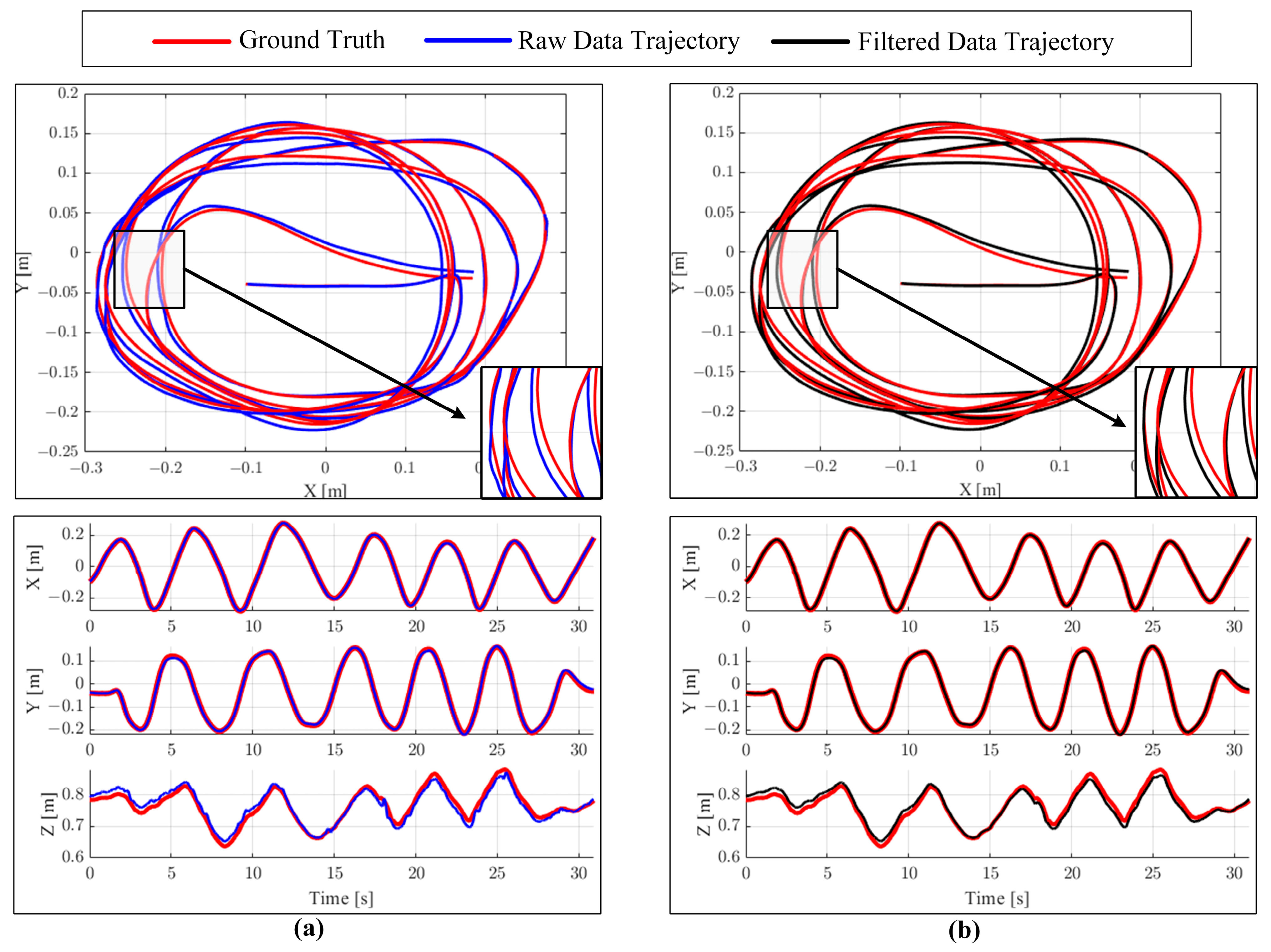
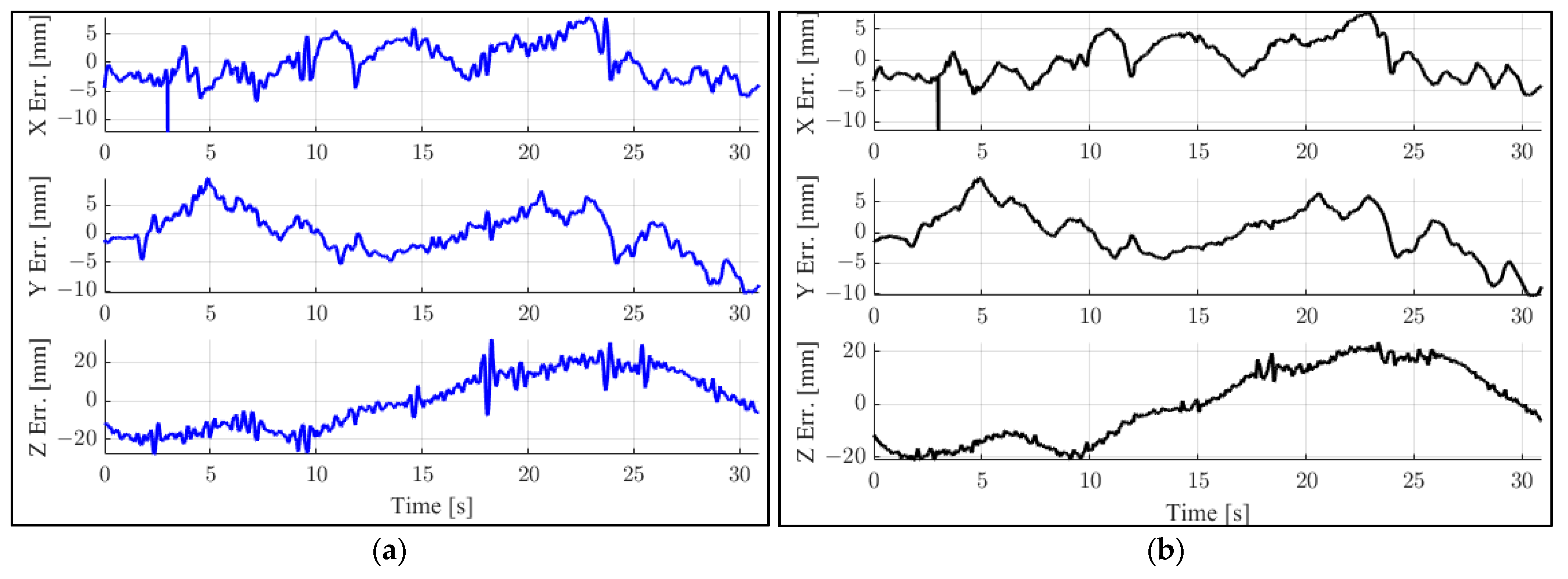
4.3. Pose Estimation Experiment

In order to verify the effectiveness of the proposed noise reduction algorithm in event-based vision tasks, in this section, we test a target using the integrated framework for event-based object position estimation presented in Section 3.3. The layout of the experimental scenario is shown in Figure 12.

A pre-calibrated DAVIS 346 event camera (346 × 260 pixels) and the Vicon motion capture system were employed in the experiments. Scaled-down models of the roadheader and the anchor drilling machine were used to simulate the actual equipment in tunneling operations. The physical models of the cantilever roadheader (900 mm × 393 mm × 308 mm) and the anchor drilling machine (913 mm × 262 mm × 404 mm) are shown in Figure 12, with a tracked robot positioned beneath the models to replicate the motions of the roadheading and bolting equipment in real tunneling scenarios. The objective of the experiment was to measure the position of the roadheader relative to the bolting machine in space. The event camera was mounted on the physical model of the bolting machine, while the target was placed on the physical model of the roadheader and moved within the camera’s field of view. The motion of the target was captured by the camera, and the corresponding events were recorded. Concurrently, positioning balls from the Vicon motion capture system were attached to the target, and the true trajectory of the target was obtained using the Vicon optical motion capture system. The partial results of pose estimation using both raw event data and filtered event data, as compared with the true values, are presented in

Table 4. Partial data for attitude estimation using raw event data.

Group	Ground Truth			Raw Data Pose			Error
	x/mm	y/mm	z/mm	x/mm	y/mm	z/mm	x/mm	y/mm	z/mm
1	−102.021	−38.690	783.997	−98.574	−39.162	785.433	−3.447	0.472	−1.436
2	136.335	−32.794	796.859	136.784	−33.207	808.408	−0.449	0.413	−11.549
3	−8.076	−194.822	746.984	−7.716	−198.890	755.323	−0.360	4.068	−8.339
4	−213.819	75.092	781.518	−212.221	66.891	785.323	−1.598	8.201	−3.805
5	184.510	76.218	825.650	182.618	71.050	829.153	1.892	5.168	−3.503
6	113.864	−180.765	690.410	116.264	−184.283	693.892	−2.400	3.518	−3.482
7	−260.360	−117.377	668.856	−260.736	−121.136	672.407	0.376	3.759	−3.551
8	−27.696	129.619	761.616	−34.266	130.458	763.206	6.570	−0.839	−1.590
9	273.760	18.117	797.805	275.008	17.510	796.989	−1.248	0.607	0.816
10	57.244	−178.920	673.903	52.542	−176.189	665.965	4.702	−2.731	7.938
11	−204.065	−35.890	693.285	−208.566	−35.867	680.658	4.501	−0.023	12.627
12	23.052	153.002	801.715	20.567	152.348	786.682	2.485	0.654	15.033
13	167.950	−139.796	786.579	164.610	−141.578	754.401	3.340	1.782	32.178
14	−225.644	−89.067	738.320	−232.302	−92.933	720.855	6.658	3.866	17.465
15	−274.243	−31.389	779.347	−273.044	−32.758	742.196	−1.199	1.369	37.151

and

Table 5. Partial data for attitude estimation using filtered event data.

Group	Ground Truth			Filtered Data Pose			Error
	x/mm	x/mm	x/mm	x/mm	y/mm	z/mm	x/mm	y/mm	z/mm
1	−102.021	−100.586	−100.586	−100.586	−39.162	785.433	−1.435	0.119	0.174
2	136.335	136.065	136.065	136.065	−33.207	808.408	0.270	−0.197	−9.834
3	−8.076	−7.196	−7.196	−7.196	−198.890	755.323	−0.880	3.807	−7.915
4	−213.819	−212.234	−212.234	−212.234	66.891	785.323	−1.585	8.475	−4.121
5	184.510	182.887	182.887	182.887	71.050	829.153	1.623	4.888	−2.542
6	113.864	116.133	116.133	116.133	−184.283	693.892	−2.269	3.376	−3.214
7	−260.360	−261.775	−261.775	−261.775	−121.136	672.407	1.415	3.911	−6.857
8	−27.696	−34.020	−34.020	−34.020	130.458	763.206	6.324	−0.504	−1.726
9	273.760	273.980	273.980	273.980	17.510	796.989	−0.220	0.429	2.924
10	57.244	52.472	52.472	52.472	−176.189	665.965	4.772	−2.456	7.421
11	−204.065	−208.350	−208.350	−208.350	−35.867	680.658	4.285	−0.392	14.149
12	23.052	20.952	20.952	20.952	152.348	786.682	2.100	0.071	16.264
13	167.950	166.029	166.029	166.029	−141.578	754.401	1.921	3.031	19.000
14	−225.644	−231.394	−231.394	−231.394	−92.933	720.855	5.750	4.358	23.491
15	−274.243	−274.063	−274.063	−274.063	−32.758	742.196	−0.180	0.017	32.700

. The comparison of the estimated trajectories against the ground truth, using data both before and after filtering, is depicted in Figure 13.

As illustrated in the first line of Figure 13, the trajectory estimated using the noise-reduced event data is closer to the actual trajectory and exhibits a smoother profile. The second line provides a quantitative comparison of errors in different directions, revealing that the position derived from the unfiltered event data exhibits significant fluctuations over a certain time interval. In contrast, the fluctuations are effectively dampened by the event data processed through the proposed algorithm. Figure 13 shows that effective events are accurately retained while noise is filtered out to the greatest extent possible by the proposed algorithm, thereby enhancing the accuracy of event line feature extraction and optimizing the overall performance of the tracking and positioning system.

To quantitatively evaluate the effect of the proposed denoising algorithm on the precision of the pose tracking system for the target, the absolute trajectory error (ATE) and the root mean square error (RMSE) of the ATE, mean error, median error, and standard deviation were calculated for both trajectory. The results of the quantitative error comparison are presented in

Table 6. Quantitative comparison with raw event data in terms of absolute trajectory error.

Data Type	Absolute Trajectory Error (mm)
	Rmse	Mean	Median	Std
Raw	15.392	14.208	15.099	5.922
Filtered	15.043	14.052	15.218	5.374

, and Figure 14 displays the ATE in the three directional components.

Based on the data presented in Table 5, the root mean square error (RMSE) of the absolute trajectory error for the event-based object tracking and localization system is reduced by 2.263% following processing with the proposed algorithm. This enhancement is attributed to the algorithm’s efficacy in mitigating the interference of noise on valid events, thereby enabling more precise and rapid extraction and tracking of event line features. Consequently, the accuracy and stability of localization are improved. The results depicted in Figure 14 indicate that after processing with the algorithm presented in this paper, the pose estimation method based on denoised event data has resulted in reduced errors in the trajectories along the X, Y, and Z axes, with particularly evident suppression of fluctuations. This improvement is attributed to the cleaner event data, which provides more accurate feature matching, thereby enhancing the overall performance of the positioning method.

5. Conclusions

Addressing the issue of the loss of partial spatio-temporal information due to the tight coupling properties of cubic spatio-temporal neighborhoods in current event camera denoising algorithms, this paper proposes a novel denoising algorithm for event cameras based on spherical spatio-temporal neighborhoods that jointly considers event density and event curvature. This method takes into account the irregular distribution of event streams in local areas of the spatio-temporal domain. By improving the spatio-temporal neighborhood, the spatio-temporal correlation of valid events is further enhanced. The method leverages the difference in spatio-temporal correlation between valid events and background noise to achieve preliminary event density denoising. Subsequently, the concept of event curvature is employed, utilizing the difference in the continuity of spatio-temporal distribution between valid events and noise events to achieve further denoising based on event curvature. The superiority of this method has been experimentally verified. Compared with other algorithms, it achieves a higher noise reduction rate (NRR) on simulated pure noise data. On the DVSNoise20 dataset, the average ESR evaluation metric of this algorithm is more than 60% higher than other algorithms. On event data from underground coal mine environments, the average ESR metric of this algorithm is more than 15% higher than other algorithms. Comparisons of the visual effects of denoising among various algorithms also indicate that this algorithm can better identify and preserve areas of high density (such as corners and edge lines, which are key features of images) while demonstrating superior denoising performance.

In response to the limitations of traditional image sensors in underground coal mine visual positioning due to harsh conditions such as low lighting, event cameras are introduced into the coal mine environment, and an object pose estimation method based on denoised events is proposed. The method processes event data through the denoising algorithm proposed in this paper. Using the OPNL method with object models and denoised event streams to provide an initial pose of the target, the association between denoised events-lines is established, and the MM estimation method is adopted to minimize the distance of denoised events–lines, thereby achieving precise optimization and tracking of the target’s pose. Experimental results demonstrate that after denoising event data, the error in pose estimation results for the target is at the millimeter level, and the root mean square error (RMSE) of the absolute trajectory error is reduced by 2.263%. Visual comparison results also show smoother and more accurate outcomes. This method can handle event noise and outliers, exhibits higher robustness against noise, and accurately estimates the pose of the target.

One of the future work directions involves research on the adaptive optimization of parameters in the denoising algorithm, with the aim of proposing a method that can automatically adjust the filter parameters according to different scenarios and requirements, thereby enhancing the generalization capability of the algorithm. Additionally, although the pose estimation method based on denoised events has been validated on a simulated experimental platform, whether it still maintains sufficiently high accuracy in actual industrial production environments is also a key focus of future research.

References

1. Zhang, L.; Wang, G.; Liu, Z.; Fu, J.; Wang, D.; Hao, Y.; Meng, L.; Zhang, J.; Zhou, Z.; Qin, J.; et al. Research of the present situation and development trend of intelligent coal mine construction market. Coal Sci. Technol. 2024, 52, 29–44. [Google Scholar]
2. Taverni, G.; Moeys, D.P.; Li, C.; Cavaco, C.; Motsnyi, V.; Bello, D.S.S.; Delbruck, T. Front and Back Illuminated Dynamic and Active Pixel Vision Sensors Comparison. IEEE Trans. Circuits Syst. II Express Briefs 2018, 65, 677–681. [Google Scholar] [CrossRef]
3. Du, Y.; Zhang, H.; Liang, L.; Zhang, J.; Song, B. Applications of Machine Vision in Coal Mine Fully Mechanized Tunneling Faces: A Review. IEEE Access 2023, 11, 102871–102898. [Google Scholar] [CrossRef]
4. Delbrück, T.; Linares-Barranco, B.; Culurciello, E.; Posch, C. Activity-driven, event-based vision sensors. In Proceedings of the 2010 IEEE International Symposium on Circuits and Systems, Paris, France, 30 May–2 June 2010. [Google Scholar]
5. Lichtsteiner, P.; Posch, C.; Delbruck, T. A 128 × 128 120 dB 15 μs latency asynchronous temporal contrast vision sensor. IEEE J. Solid-State Circuits 2008, 43, 566–576. [Google Scholar] [CrossRef]
6. Gallego, G.; Delbrück, T.; Orchard, G.; Bartolozzi, C.; Taba, B.; Censi, A.; Leutenegger, S.; Davison, A.J.; Conradt, J.; Scaramuzza, D.; et al. Event-based vision: A survey. IEEE Trans. Pattern Anal. Mach. Intell. 2020, 44, 154–180. [Google Scholar] [CrossRef] [PubMed]
7. Hu, Y.; Liu, S.-C.; Delbruck, T. v2e: From video frames to realistic DVS events. In Proceedings of the IEEE/CVF Conference on Computer Vision and Pattern Recognition, Nashville, TN, USA, 20–25 June 2021. [Google Scholar]
8. Delbruck, T. Frame-free dynamic digital vision. In Proceedings of the International Symposium on Secure-Life Electronics Advanced Electronics for Quality Life and Society, Tokyo, Japan, 6–7 March 2008; Volume 1. [Google Scholar]
9. Czech, D.; Orchard, G. Evaluating noise filtering for event-based asynchronous change detection image sensors. In Proceedings of the 2016 6th IEEE International Conference on Biomedical Robotics and Biomechatronics (BioRob), Singapore, 26–29 June 2016. [Google Scholar]
10. Liu, H.; Brandli, C.; Li, C.; Liu, S.C.; Delbruck, T. Design of a spatiotemporal correlation filter for event-based sensors. In Proceedings of the 2015 IEEE International Symposium on Circuits and Systems (ISCAS), Lisbon, Portugal, 24–27 May 2015. [Google Scholar]
11. Khodamoradi, A.; Kastner, R. O(N)-Space Spatiotemporal Filter for Reducing Noise in Neuromorphic Vision Sensors. IEEE Trans. Emerg. Top. Comput. 2018, 9, 15–23. [Google Scholar] [CrossRef]
12. Feng, Y.; Lv, H.; Liu, H.; Zhang, Y.; Xiao, Y.; Han, C. Event Density Based Denoising Method for Dynamic Vision Sensor. Appl. Sci. 2020, 10, 2024. [Google Scholar] [CrossRef]
13. Wang, Y.; Du, B.; Shen, Y.; Wu, K.; Zhao, G.; Sun, J.; Wen, H. EV-gait: Event-based robust gait recognition using dynamic vision sensors. In Proceedings of the IEEE/CVF Conference on Computer Vision and Pattern Recognition, Long Beach, CA, USA, 15–20 June 2019. [Google Scholar]
14. Duan, P.; Wang, Z.W.; Shi, B.; Cossairt, O.; Huang, T.; Katsaggelos, A.K. Guided event filtering: Synergy between intensity images and neuromorphic events for high performance imaging. IEEE Trans. Pattern Anal. Mach. Intell. 2021, 44, 8261–8275. [Google Scholar]
15. Lagorce, X.; Orchard, G.; Galluppi, F.; Shi, B.E.; Benosman, R.B. HOTS: A Hierarchy of Event-Based Time-Surfaces for Pattern Recognition. IEEE Trans. Pattern Anal. Mach. Intell. 2016, 39, 1346–1359. [Google Scholar] [CrossRef] [PubMed]
16. Baldwin, R.W.; Almatrafi, M.; Kaufman, J.R.; Asari, V.; Hirakawa, K. Inceptive event time-surfaces for object classification using neuromorphic cameras. In Proceedings of the Image Analysis and Recognition: 16th International Conference, ICIAR 2019, Waterloo, ON, Canada, 27–29 August 2019; Proceedings, Part II 16. Springer International Publishing: Berlin/Heidelberg, Germany, 2019. [Google Scholar]
17. Duan, P.; Wang, Z.W.; Zhou, X.; Ma, Y.; Shi, B. EventZoom: Learning to denoise and super resolve neuromorphic events. In Proceedings of the IEEE/CVF Conference on Computer Vision and Pattern Recognition, Nashville, TN, USA, 20–25 June 2021. [Google Scholar]
18. Baldwin, R.W.; Almatrafi, M.; Asari, V.; Hirakawa, K. Event Probability Mask (EPM) and Event Denoising Convolutional Neural Network (EDnCNN) for Neuromorphic Cameras. In Proceedings of the IEEE/CVF Conference on Computer Vision and Pattern Recognition, Seattle, WA, USA, 13–19 June 2020. [Google Scholar]
19. Fang, H.; Wu, J.; Li, L.; Hou, J.; Dong, W.; Shi, G. AEDNet: Asynchronous Event Denoising with Spatial-Temporal Correlation among Irregular Data. In Proceedings of the 30th ACM International Conference on Multimedia, Lisbon, Portugal, 10–14 October 2022. [Google Scholar]
20. Hoffmann, R.; Weikersdorfer, D.; Conradt, J. Autonomous indoor exploration with an event-based visual SLAM system. In Proceedings of the 2013 European Conference on Mobile Robots, Barcelona, Spain, 25–27 September 2013. [Google Scholar]
21. Kueng, B.; Mueggler, E.; Gallego, G.; Scaramuzza, D. Low-latency visual odometry using event-based feature tracks. In Proceedings of the 2016 IEEE/RSJ International Conference on Intelligent Robots and Systems (IROS), Daejeon, Republic of Korea, 9–14 October 2016. [Google Scholar]
22. Censi, A.; Scaramuzza, D. Low-Latency Event-Based Visual Odometry. In Proceedings of the IEEE International Conference on Robotics and Automation (ICRA), Hong Kong, China, 31 May–7 June 2014; pp. 703–710. [Google Scholar]
23. Kim, H.; Leutenegger, S.; Davison, A.J. Real-time 3D reconstruction and 6-DoF tracking with an event camera. In Proceedings of the Computer Vision–ECCV 2016: 14th European Conference, Amsterdam, The Netherlands, 11–14 October 2016; Springer International Publishing: Berlin/Heidelberg, Germany, 2016. [Google Scholar]
24. Rebecq, H.; Horstschaefer, T.; Gallego, G.; Scaramuzza, D. EVO: A Geometric Approach to Event-Based 6-DOF Parallel Tracking and Mapping in Real Time. IEEE Robot. Autom. Lett. 2016, 2, 593–600. [Google Scholar] [CrossRef]
25. Vidal, A.R.; Rebecq, H.; Horstschaefer, T.; Scaramuzza, D. Ultimate SLAM? Combining Events, Images, and IMU for Robust Visual SLAM in HDR and High-Speed Scenarios. IEEE Robot. Autom. Lett. 2018, 3, 994–1001. [Google Scholar] [CrossRef]
26. Gehrig, D.; Rebecq, H.; Gallego, G.; Scaramuzza, D. EKLT: Asynchronous photometric feature tracking using events and frames. Int. J. Comput. Vis. 2020, 128, 601–618. [Google Scholar] [CrossRef]
27. Hidalgo-Carrió, J.; Gallego, G.; Scaramuzza, D. Event-aided direct sparse odometry. In Proceedings of the IEEE/CVF Conference on Computer Vision and Pattern Recognition, New Orleans, LA, USA, 18–24 June 2022. [Google Scholar]
28. Reverter Valeiras, D.; Orchard, G.; Ieng, S.H.; Benosman, R.B. Neuromorphic event-based 3d pose estimation. Front. Neurosci. 2016, 9, 522. [Google Scholar] [CrossRef] [PubMed]
29. Reverter Valeiras, D.; Kime, S.; Ieng, S.H.; Benosman, R.B. An event-based solution to the perspective-n-point problem. Front. Neurosci. 2016, 10, 208. [Google Scholar]
30. Jawaid, M.; Elms, E.; Latif, Y.; Chin, T.-J. Towards Bridging the Space Domain Gap for Satellite Pose Estimation using Event Sensing. In Proceedings of the 2023 IEEE International Conference on Robotics and Automation (ICRA), London, UK, 29 May–2 June 2023. [Google Scholar]
31. Liu, Q.; Xing, D.; Tang, H.; Ma, D.; Pan, G. Event-based Action Recognition Using Motion Information and Spiking Neural Networks. In Proceedings of the Thirtieth International Joint Conference on Artificial Intelligence {IJCAI-21}, Montreal, QC, Canada, 19–27 August 2021. [Google Scholar]
32. Yu, N.; Ma, T.; Zhang, J.; Zhang, Y.; Bao, Q.; Wei, X.; Yang, X. Adaptive Vision Transformer for Event-Based Human Pose Estimation. In Proceedings of the 32nd ACM International Conference on Multimedia, Melbourne, VIC, Australia, 28 October–1 November 2024. [Google Scholar]
33. Liu, Z.; Guan, B.; Shang, Y.; Yu, Q.; Kneip, L. Line-Based 6-DoF Object Pose Estimation and Tracking with an Event Camera. IEEE Trans. Image Process. 2024, 33, 4765–4780. [Google Scholar] [CrossRef] [PubMed]
34. Zhao, G.; Du, Z.; Guo, Z.; Ma, H. VRHCF: Cross-Source Point Cloud Registration via Voxel Representation and Hierarchical Correspondence Filtering. arXiv 2024, arXiv:2403.10085. [Google Scholar]
35. Tombari, F.; Salti, S.; Di Stefano, L. Unique signatures of histograms for local surface description. In Proceedings of the Computer Vision–ECCV 2010: 11th European Conference on Computer Vision, Heraklion, Greece, 5–11 September 2010; Proceedings, Part III 11. Springer: Berlin/Heidelberg, Germany, 2010. [Google Scholar]
36. Lei, H.; Akhtar, N.; Mian, A. Octree guided cnn with spherical kernels for 3D point clouds. In Proceedings of the IEEE/CVF Conference on Computer Vision and Pattern Recognition, Long Beach, CA, USA, 15–20 June 2019. [Google Scholar]
37. Wang, Z.; Hu, J.; Shi, Y.; Cai, J.; Pi, L. Target Fitting Method for Spherical Point Clouds Based on Projection Filtering and K-Means Clustered Voxelization. Sensors 2024, 24, 5762. [Google Scholar] [CrossRef] [PubMed]
38. Yu, Q.; Xu, G.; Cheng, Y. An efficient and globally optimal method for camera pose estimation using line features. Mach. Vis. Appl. 2020, 31, 48. [Google Scholar] [CrossRef]
Figure 1. The event data captured by the DAVIS346 camera were temporally projected to generate a 2D event frame image, with positive and negative polarities distinguished by red and blue colors, respectively. Notably, background noise is intermixed with valid events in both the spatio-temporal domain and within the event frame.
Mathematics 13 01198 g001
Figure 2. Event frame and RGB grayscale frame captured by DAVIS346 event camera were used in coal mine environment. (a) Event frame; (b) RGB grayscale frame.
Mathematics 13 01198 g002
Figure 3. Schematic of the cubic spatio-temporal neighborhood. The red pixel denotes an event e i occurring at a specific moment. The yellow region represents the spatial neighborhood of this event, while Δ t indicates the temporal neighborhood associated with this event. The combination of the temporal and spatial neighborhoods constitutes the spatio-temporal neighborhood Ω Δ t L .
Mathematics 13 01198 g003
Figure 4. Schematic of a spherical spatio-temporal neighborhood. The red dots represent positive polar events and the blue dots represent negative polar events. The green pixels represent events occurring at a specific moment in time. By considering both the temporal and spatial (pixel) dimensions, we construct a spherical spatio-temporal neighborhood using the concepts of penalty coefficients and KD-tree algorithms.
Mathematics 13 01198 g004
Figure 5. Examples of curvature-based noise cancellation methods, with color values representing different curvature values. Valid events (green) can be fitted on the same surface, having approximately equal curvature values. Noise events (purple), on the other hand, cannot be fitted to the same surface as neighboring events and have different curvature than valid events.
Mathematics 13 01198 g005
Figure 6. PNL problem diagram.
Mathematics 13 01198 g006
Figure 7. The flowchart of the proposed framework for object pose tracking and estimation based on event denoising.
Mathematics 13 01198 g007
Figure 8. Visual comparison of different denoising algorithms in a pure noise processing task. All event frames are 30 ms in duration. Here, we do not consider event polarity, and white dots are simulated BA noise. Event frames at identical locations are magnified to facilitate comparison (the red box in the lower left corner).
Mathematics 13 01198 g008
Figure 9. Denoising visualization results on the DVSNoise20 (event frame duration of 30 ms). The initial row depicts the event frame resulting from the projection of raw event data. Subsequent rows, namely the second through sixth, illustrate the outcomes of event data processing via distinct denoising algorithms.
Mathematics 13 01198 g009
Figure 10. Experimental platform for event camera data acquisition in underground environment of coal mine. (a) The digging face; (b) The fully mechanized face.
Mathematics 13 01198 g010
Figure 11. Visualization of denoising outcomes on event data acquired in a laboratory setting that simulates an underground coal mine environment (event frame duration of 30 ms). Arranged in descending order, the event frames showcase projections derived from the original data and subsequent data that have been subjected to various noise reduction algorithms.
Mathematics 13 01198 g011
Figure 12. Experimental platform construction for target attitude estimation and tracking.
Mathematics 13 01198 g012
Figure 13. Experimental results on position estimation and tracking. The first row provides a qualitative comparison of the overall trajectories, while the second row offers a quantitative comparison of the translational estimates of the trajectories. (a) Comparison of trajectory and truth value of attitude estimation using raw event data. (b) The trajectory of attitude estimation is compared with the truth value using filtered event data.
Mathematics 13 01198 g013
Figure 14. Schematic diagram of absolute trajectory error in three directions. (a) The ATE obtained by the pose estimation method using raw event data. (b) The ATE obtained by the pose estimation method using filtered event data.
Mathematics 13 01198 g014