Unit Size Determination for Exploratory Brain Imaging Analysis: A Quest for a Resolution-Invariant Metric

Abstract

Defining an adequate unit size is often crucial in brain imaging analysis, where datasets are complex, high-dimensional, and computationally demanding. Unit size refers to the spatial resolution at which brain data is aggregated for analysis. Optimizing unit size in data aggregation requires balancing computational efficiency in handling large-scale data sets with the preservation of brain activity patterns, minimizing signal dilution. We propose using the Calinski–Harabasz index, demonstrating its invariance to sample size changes due to varying image resolutions when no distributional differences are present, while the index effectively identifies an appropriate unit size for detecting suspected regions in image comparisons. The resolution-independent metric can be used for unit size evaluation, ensuring adaptability across different imaging protocols and modalities. This study enhances the scalability and efficiency of brain imaging research by providing a robust framework for unit size optimization, ultimately strengthening analytical tools for investigating brain function and structure.

1. Introduction

Defining an adequate unit size is a crucial step in brain imaging analysis, where data is inherently complex, high-dimensional, and computationally intensive. Unit size refers to the spatial resolution at which the brain is analyzed, ranging from individual voxels to aggregated regions such as regions of interest (ROIs). The choice of unit size has substantial implications for both the interpretability of results and the computational feasibility of downstream analyses.

In this paper, we investigate a resolution-free metric for data aggregation (combining the data points) in brain imaging, which aggregates large three-dimensional voxel data into more manageable unit sizes. Maintaining distributional properties of data during data aggregation or fission [1] is not of particular interest of this paper. Rather, we aim to propose a relevant criterion for adjusting resolution to determine an appropriate unit size for subsequent analysis, such as clustering. Ultimately, this approach does not require prior knowledge of brain structures and, thus, it may be suitable for initial exploratory analysis.

While ROI-based approaches efficiently reduce dimensionality by averaging signals within predefined brain regions [2], they require prior knowledge and may obscure localized effects. This limitation makes them less suitable for initial exploratory analyses, where a more flexible and data-driven approach is needed. Voxel-based methods, such as voxel-based morphometry (VBM) [3] provide fine-grained spatial resolution, enabling detailed anatomical analysis. However, they often suffer from high computational costs and increased susceptibility to noise. On the other hand, grid-based methods segment the brain into uniform cubic regions, offering a straightforward approach to defining unit sizes. While fine-grained grids preserve detailed information, they significantly increase the number of regions, making clustering, machine learning, and statistical modeling computationally expensive and memory-intensive. Conversely, overly large grids obscure finer-scale features, reducing sensitivity to localized effects.

An optimal unit size must balance the trade-off between preserving relevant signal patterns and maintaining computational efficiency. Thus, we propose two essential conditions for defining an adequate unit size in brain imaging:

i.

Minimizing signal dilution for detecting meaningful regional differences—The unit size should be small enough to capture localized biological variations that distinguish different phenotypic traits or pathological conditions. Overly large units may obscure these critical differences, reducing the ability to accurately characterize relevant biological patterns.

ii.

Optimizing computational efficiency—The unit size should be large enough to prevent unnecessary computational overhead. Brain imaging datasets, such as those from functional magnetic resonance imaging (fMRI) or diffusion tensor imaging (DTI), often contain millions of data points. Aggregating adjacent voxels into larger units can reduce the computational burden while preserving data fidelity.

To illustrate the importance of computational efficiency, consider the $k$-means clustering algorithm, commonly used in brain imaging for segmentation and pattern identification. Each iteration of $k$-means requires $O\left(nkd\right)$ computations, where $n$is the number of data points, $k$ is the number of clusters, and $d$ is the data dimensionality. Given the NP-hard nature of $k$-means [4], the problem becomes computationally intractable as $n$ increases. Doubling the number of units approximately doubles the computational time, making unit size a critical factor in large-scale imaging studies. Careful aggregation of voxels into appropriate units can significantly improve computational efficiency without losing meaningful information.

Another key challenge in brain imaging is the need for a scale- and sample-size-independent metric for evaluating unit size. Such a metric should remain invariant to the merging or splitting of subunits and be adaptable to variations in spatial resolution due to differences in imaging modalities or preprocessing pipelines. At the same time, it must be sensitive enough to indicate when unit size is optimal for capturing relevant neural activity or structural characteristics.

In this paper, we propose a novel framework for determining a desirable unit size that balances the detection of meaningful patterns relevant to the disease of interest and computational efficiency. We aim to evaluate the Calinski–Harabasz index [5] as a metric for guiding data aggregation in brain imaging analysis, particularly focusing on its stability with respect to varying sample sizes. Our goal is to develop a preprocessing framework that simplifies high-dimensional brain imaging data by determining proper unit sizes, reducing computational burden while preserving essential information for downstream analyses. By selecting an appropriate unit size, we seek to enhance the efficiency and interpretability of brain imaging studies, ultimately facilitating deeper insights into neural function at meaningful spatial scales.

2. Methods

Suppose we have $K$ groups of interest and our objective is to identify brain regions that most clearly distinguish among them in the framework of supervised methods. For instance, we may be interested in identifying brain regions that differentiate case and control groups. To achieve this, we use a clustering approach to uncover regions most strongly associated with group-level differences. Minimizing signal dilution in this context translates to determining an optimal unit size that effectively captures differences between $K$ groups. However, as data aggregation is performed, the dataset size continuously changes. Therefore, it is crucial to establish a robust metric that remains minimally influenced by changes in sample size.

Herein, we propose the Calinski–Harabasz index (CHI) as such a metric. The index, in its original role, provides a robust way to quantify the separation between clusters while accounting for within-cluster variance, making it a valuable metric for evaluating clustering performance [5]. We provide a detailed explanation and demonstrate analytically that, under the absence of true group differences, the CHI remains independent of sample size. Conversely, when genuine group differences exist, the CHI clearly and distinctly highlights these differences at or around appropriate unit sizes.

Let ${\mathbf{Y}}_{kj}={\left(Y_{1kj},\dots ,Y_{pkj}\right)}^T$ represent the $j$-th data point in group $k \left(k=1,\dots ,K\right),$ where each data point is a$p$-dimensional vector with variance $\mathrm{V}\mathrm{a}\mathrm{r}\left({\mathbf{Y}}_{kj}\right)=\mathsf{\Sigma }$. The full dataset is represented by $\mathcal{Y}$ of dimension $N\times p$. We express the transposed data set as

$${\mathcal{Y}}^T=\left[{\mathcal{Y}}_1^T,\dots ,{\mathcal{Y}}_K^T\right],$$

where ${\mathcal{Y}}_k^T$ is the data in group $k$ ($k=1,\dots ,K$). Let $C_k$ denote the set of data points in group $k$, with cardinality $\left|C_k\right|=n_k$. Thus, the total number of data points in the data set is $N={\sum }_{k=1}^K{n}_k$. The mean vector of group $k$ is ${\overline{\mathbf{Y}}}_k={{\displaystyle \frac{1}{n_k}}\mathcal{Y}}_k^T{1}_{n_k}^T$, where $1_n$ is the $n$-dimensional all-ones vector. Similarly, the overall mean vector of the data set is $\overline{\mathbf{Y}}$ ${={\displaystyle \frac{1}{N}}\mathcal{Y}}^T{1}_N^T$. The CHI is expressed as the ratio

$$H={\displaystyle \frac{{\sum }_{k=1}^K\left|C_k\right|{\hspace{0.17em}‖{\overline{\mathbf{Y}}}_k-\overline{\mathbf{Y}}‖}^2/\hspace{0.17em}\left(K-1\right)}{{\sum }_{k=1}^K{\sum }_{\mathrm{Y}\in C_k}{‖\mathbf{Y}-{\overline{\mathbf{Y}}}_k‖}^2\hspace{0.17em}/\hspace{0.17em}\left(N-K\right)}},$$

(1)

where ${‖\cdot ‖}^2$ denotes the Euclidian $L_2$ norm. Alternatively, $H$is expressed as

$$H={\displaystyle \frac{\mathrm{t}\mathrm{r}\left({\mathbf{S}}_B\right)/\hspace{0.17em}\left(K-1\right)}{\mathrm{t}\mathrm{r}\left({\mathbf{S}}_W\right)/\hspace{0.17em}\left(N-K\right)}}={\displaystyle \frac{\left\{{\sum }_{k=1}^K{\sum }_{j=1}^{n_i}{\left({\overline{Y}}_{1k.}-{\overline{Y}}_{1..}\right)}^2+\cdots +{\sum }_{k=1}^K{\sum }_{j=1}^{n_i}{\left({\overline{Y}}_{pk.}-{\overline{Y}}_{p..}\right)}^2\right\}/\left(K-1\right)}{\left\{{\sum }_{k=1}^K{\sum }_{j=1}^{n_i}{\left(Y_{1kj}-{\overline{Y}}_{1k.}\right)}^2+\cdots +{\sum }_{k=1}^K{\sum }_{j=1}^{n_i}{\left(Y_{pkj}-{\overline{Y}}_{pk.}\right)}^2\right\}/\left(N-K\right)}},$$

where ${\mathbf{S}}_B={\sum }_{k=1}^K\left|C_k\right| ({\overline{\mathbf{Y}}}_k-\overline{\mathbf{Y}}){\left({\overline{\mathbf{Y}}}_k-\overline{\mathbf{Y}}\right)}^T, {\mathbf{S}}_W={\sum }_{k=1}^K{\sum }_{\mathbf{Y}\in C_k}\left(\mathbf{Y}-{\overline{\mathbf{Y}}}_k\right) {\left(\mathbf{Y}-{\overline{\mathbf{Y}}}_k\right)}^T$, and $\mathrm{t}\mathrm{r}$ denotes the trace of a matrix. Since the CHI is defined using the trace of scatter matrices, it is well known to be invariant under the orthogonal transformation of the data. We state this property in Lemma 1 and a proof is given in the Appendix A.

Lemma 1.

The Calinkski–Harabasz Index value remains unchanged by the orthogonal transformation the data.

For the data aggregation, we consider the following setup. Aggregated data for group $k$ are denoted as ${\tilde{\mathbf{Y}}}_{k1},\dots ,{\tilde{\mathbf{Y}}}_{k{\tilde{n}}_k}$, where ${\tilde{n}}_k$ is $\lceil n_k/d \rceil$ and $d$ is the number of original datapoints without replacement aggregated into a single data point, i.e., ${\tilde{\mathbf{Y}}}_{ki}={\displaystyle \frac{1}{d}}{\sum }_{j\in s_i}{\mathbf{Y}}_{kj}$, where $s_i (i=1,\dots$, ${\tilde{n}}_k)$ is a subset of $\left\{1,\dots ,n_k\right\}$ with cardinality $d$. The total number of aggregated data points across all groups is given by ${\sum }_{k=1}^K{\tilde{n}}_k=\tilde{N}.$At the element level, ${\tilde{\mathbf{Y}}}_{ki}$ is expressed as ${\tilde{\mathbf{Y}}}_{ki}={\left({\tilde{Y}}_{1ki},\dots , {\tilde{Y}}_{pki}\right)}^T$. Technically, the subset $s_i$ can be chosen randomly from the index set but, for simplicity, we can consider that aggregations are carried out over $d$ consecutive indices. If $n_k$ is not divisible by $d$, only the last element ${\tilde{\mathbf{Y}}}_{k{\tilde{n}}_k}$ is formed by fewer than $d$ original data points. Without loss of generality, consider that $n_k$ is divisible by $d$, thus we assume all aggregated data points comprise $d$ original data points. Consequently, the variance of the aggregated data point is $\mathrm{V}\mathrm{a}\mathrm{r}\left({\tilde{\mathbf{Y}}}_{ki}\right)={\displaystyle \frac{1}{d}}\mathsf{\Sigma }$. For the subsequent argument, we assume that ${\mathbf{Y}}_{ki}$ has a multivariate normal distribution with the mean $\mathrm{E}\left({\mathbf{Y}}_{ki}\right)={\mathit{\mu }}_k$, for all $k=1,\dots ,K$. Now, we state the following result.

Theorem 1.

For independent observations ${\mathit{Y}}_{ki}$ following a multinormal distribution $(k=1,\dots ,K, i=1,\dots n_k)$, suppose $E\left({\mathit{Y}}_{ki}\right)=\mathit{\mu }$ and $Var\left({\mathit{Y}}_{ki}\right)=\mathit{\Sigma }$ for all $k=1,\dots ,K$. Then, the $m$-th moments of the CHI for a positive integer $m$ is asymptotically independent of the sample size.

The proof is given in the Appendix A. Theorem 1 states that the rate of convergence of the moments of the CHI is independent of the sample size upon the data aggregation under the assumption that all groups have the same distribution, i.e., aggregation of data will not change the CHI’s distribution asymptotically. Regarding the usage of the CHI, it is important to note that the assumption of independence between observations is not strictly required. In practice, this assumption is often unrealistic, particularly in structured or correlated data settings. However, our theorem demonstrates that the CHI remains relatively stable and less sensitive to variations in sample size, suggesting its usefulness for comparisons across different sample size conditions.

Now, with original $N\times p$ data, consider only one variate $l$ among $p$ variates, $(l=1,\dots .,p)$. We define

$$\begin{array}{c}{S}_{B_l}={\displaystyle \sum _{k=1}^K}{\displaystyle \sum _{j=1}^{n_i}}{\left({\overline{Y}}_{pk.}-{\overline{Y}}_{p..}\right)}^2/(K-1),\\ S_{w_l}={\displaystyle \sum _{k=1}^K}{\displaystyle \sum _{j=1}^{n_i}}{\left(Y_{lkj}-{\overline{Y}}_{lk.}\right)}^2 /\left(N-K\right),\\ H_l={\displaystyle \frac{{\sum }_{k=1}^K{\sum }_{j=1}^{n_i}{\left({\overline{Y}}_{lk.}-{\overline{Y}}_{l..}\right)}^2/\left(K-1\right)}{{\sum }_{k=1}^K{\sum }_{j=1}^{n_i}{\left(Y_{lkj}-{\overline{Y}}_{lk.}\right)}^2/\left(N-K\right)}},\end{array}$$

(2)

where $S_{w_l}$ is the unbiased estimator of ${\sigma }_l^2.$ Suppose that group $k^{*}$ among $K$ groups consists of a mixture of two distributions, i.e., $N({\mu }_1, {\sigma }_l^2)$ and $N({\mu }_2, {\sigma }_l^2)$, where ${\mu }_1\ne {\mu }_2$. Under these conditions, we have the following result.

Theorem 2.

Consider the same distributional assumptions as Theorem 1, except that data or image of group $k^{*}$ consists of the two mixed distributions. Then, for sufficiently large $n_{k^{*}}$, the expectation of $H_l$ satisfies $E\left(H_l\right)\le E\left(S_{B_l}\right)/ {\sigma }_l^2$.

Theorem 2 can be easily provable by the standard ANOVA results [6]. Specifically, when a group of the data consists of mixed distributions, the estimator $S_{w_l}$ is an estimator based on a reduced model or underspecified model. In that circumstance, the underspecified model provides an inflated variance estimate, which leads to the result stated in Theorem 2, using the fact that the numerator and the denominator of the CHI are independent. The detailed proof is given in the Appendix A. Now, the following corollary extends the result in Theorem 2 for general $p$ variates.

Corollary 1.

Consider the same distributional assumptions as Theorem 1, except that data or image of group $k^{*}$ consists of the two mixed distributions. Then, for sufficiently large $n_{k^{*}}$, the expectation of $H$ satisfies $E\left(H\right)\le E\left({\displaystyle \frac{{\mathit{S}}_B}{K-1}}\right)/tr\left(\mathit{\Sigma }\right)$.

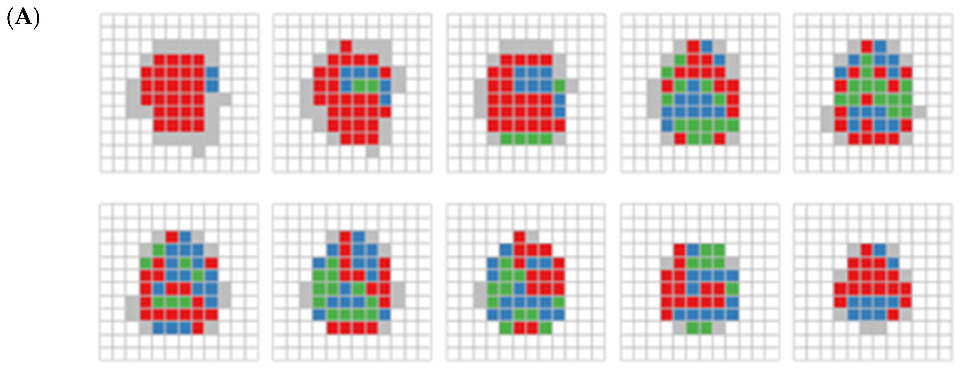
The proof is given in the Appendix A. Corollary 1 indicates that the CHI statistic yields smaller values in the presence of mixed distributions than when these mixtures are absent. Data aggregation can increase the presence of mixed distributions, as illustrated in Figure 1. Initially, data consisting of two distributions becomes several distributions after aggregation, causing a decrease in the CHI statistic due to model underspecification. On the other hand, as aggregation progresses, we may observe that the number of mixed distributions gradually declines due to a reduced number of data points.

Conversely, if the data undergoes splitting starting from the optimal unit size, the number of data points increases, preserving the two distinct distributions. This splitting process leads to a sharp increase in the CHI values. The simulation in the next section demonstrates this phenomenon, showing a sharp rise or “elbow point” in the CHI values around the optimal unit size.

3. Simulation

We investigate the behavior of the CHI under data aggregation through simulation. In this simulation, we compare two groups of synthetic 3D image data (a control image and a case image), where the control and case images are different not at the pixel level but at the level of certain blocks of uniformly sized squares. Both image groups consist of synthetic image data containing 3600 pixels arranged in a $60\times 60$ grid. Every pixel contains 3 features ($p=3$), independently generated from a multi-normal distribution. Initially, both the control and case images are independently generated with identical distributions. The mean vector is set to (1, 1, 2) and the covariance matrix is constructed with a correlation of 0.2 between features and a diagonal standard deviation of 1. Then, contamination is introduced into the case image as follows. In the first scenario, certain blocks within the case image are replaced with data generated from a shifted mean vector (2, 2, 3). The contaminated regions consist of $4\times 4$ pixel blocks, resulting in 225 total number of candidate blocks for contamination. From these 225 blocks, 10 to 30% are randomly selected for contamination. This localized disturbance creates differences between the control and case images at the block level.

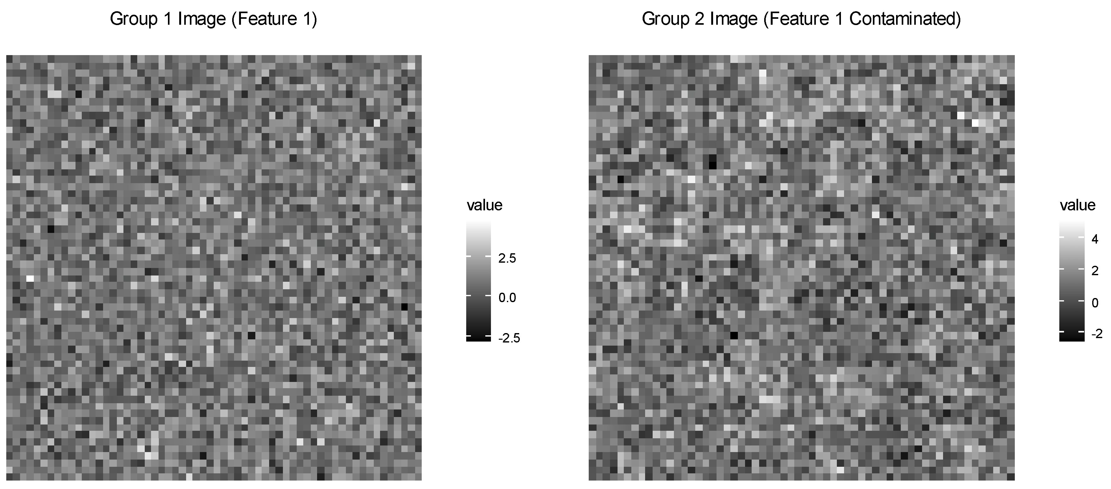
The visualization (Figure 2) extracts the first feature from each image and displays it using a grayscale gradient, with dark pixels indicating low values and bright pixels indicating high values. In the figure, the control image appears as a relatively uniform grayscale texture with random noise, while the case image shows some brighter patches corresponding to contaminated blocks.

We perform an analysis by dividing each image into blocks of varying sizes: 1, 2, 4, 5, 10, 15, and 20 pixels per block. For each block size, we calculate the mean values of the features within each block, resulting in reduced data matrices for both image groups. We then compute the CHI for these aggregated blocks to provide insights into how contamination affects the CHI at various aggregation levels.

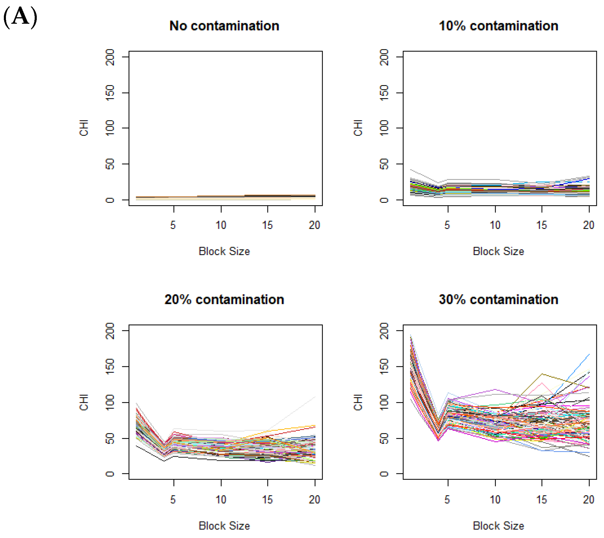
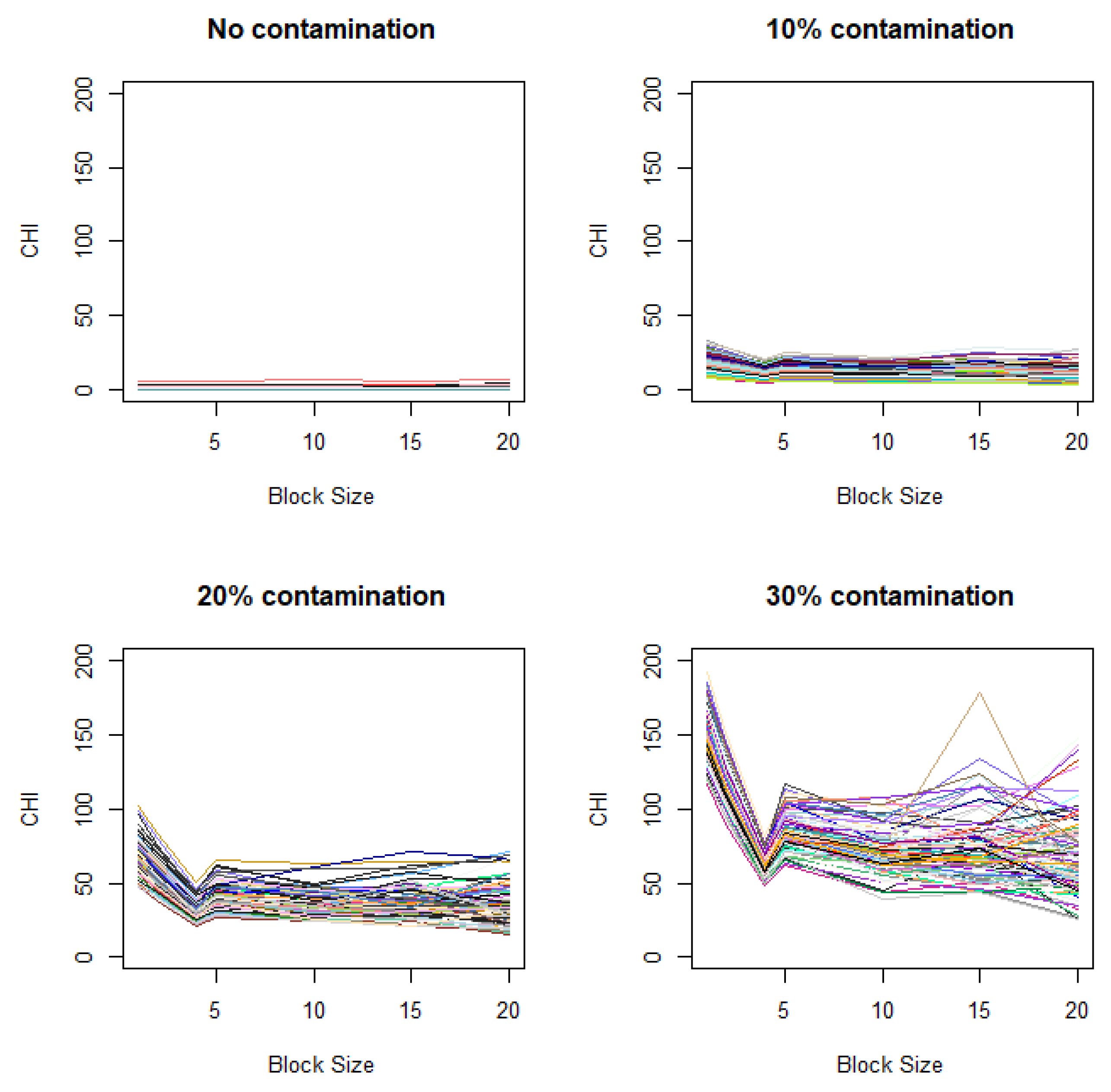
The changes in the CHI values resulting from varying levels of data aggregations are displayed in Figure 3A, based on 100 simulations for each plot. Figure 3A displays the CHI value changes across different contamination rates, with the fixed contamination unit size of $4\times 4$. When there is no difference in distributions between the control and case images (i.e., in the absence of contamination), the CHI values remain relatively low with no notable patterns observed. When contaminated blocks are present in the case images, the figure clearly shows a distinctive pattern, where the CHI values substantially increase during data splitting (moving from right to left on the x-axis in Figure 3A). Clear elbows appear at 4 on the x-axis, even with relatively low contamination rates (e.g., 10%). When the level of contamination is higher, the overall patterns remain similar, except that the elbow points become more pronounced.

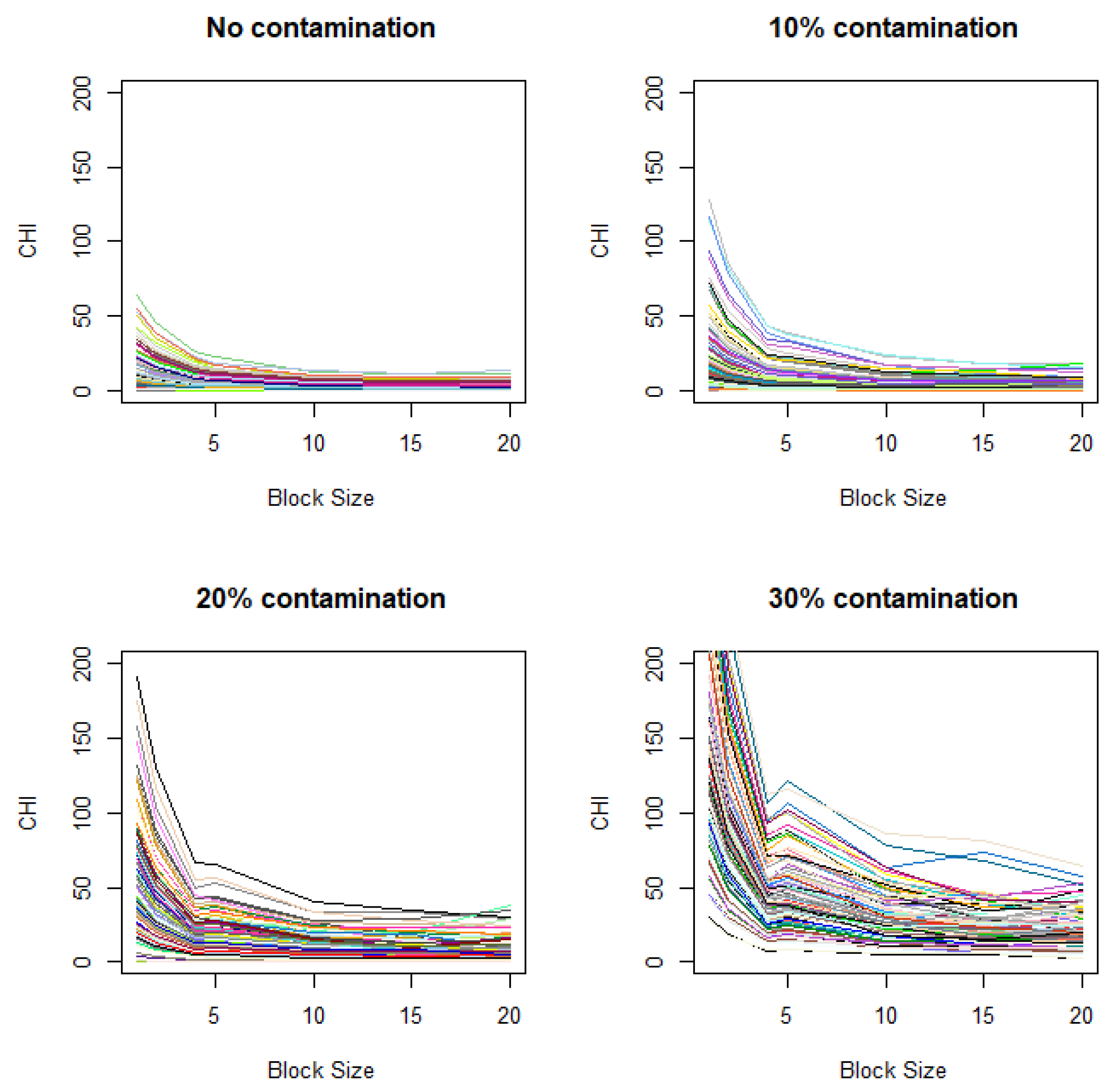
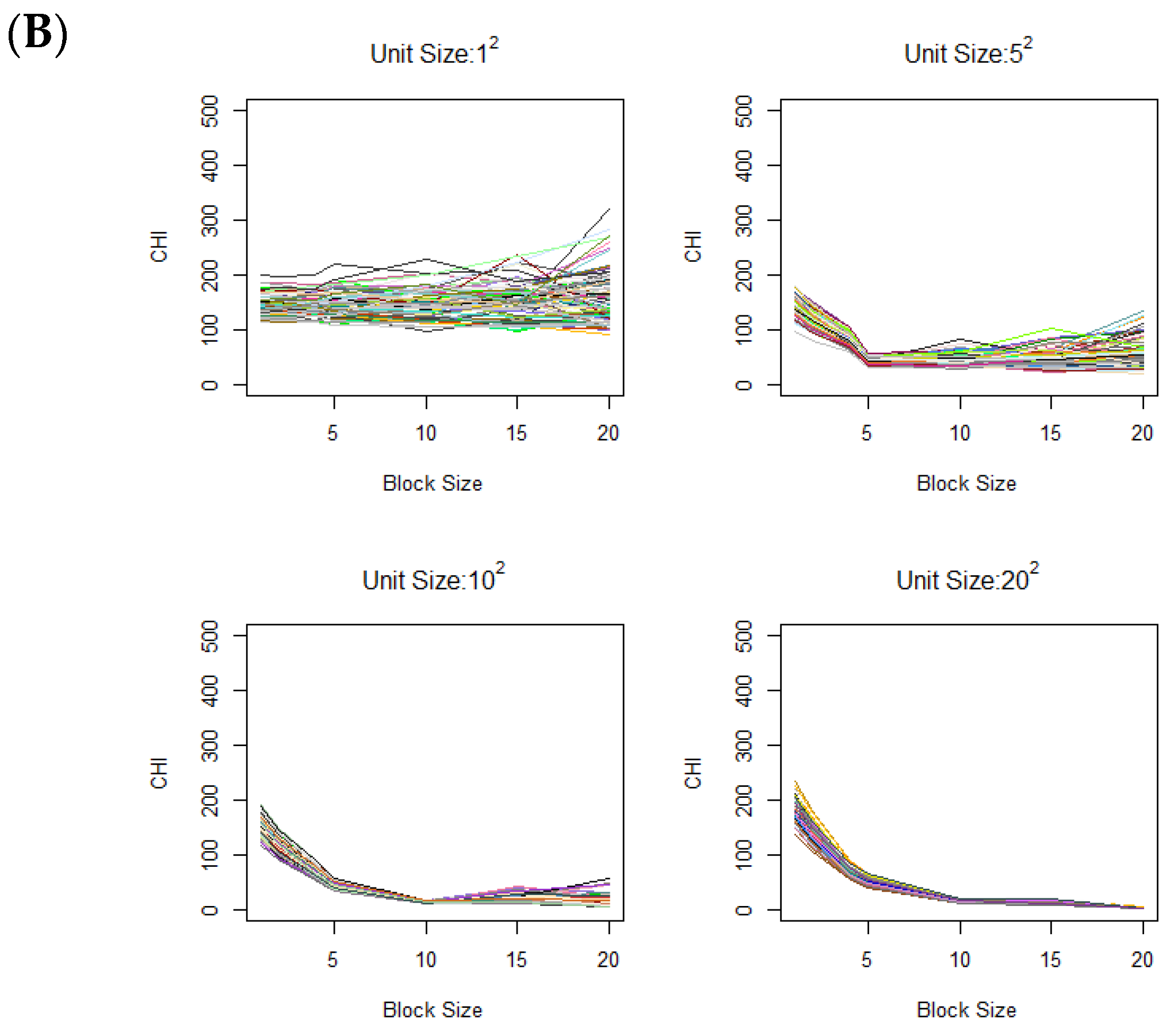
As another scenario, we also vary the unit size of contamination, i.e., the vertical lengths of the square contamination units are set to 1, 5, 10, and 20, while the overall contamination rate remains fixed at 30%. Figure 3B shows the CHI value changes across different contamination unit sizes. Clear elbows appear at respective contamination unit sizes. Notably, when the unit size is large, there is a gradual increase without a distinctive elbow as explained under Corollary 1.

These simulations are based on the assumptions that closely align with those for ANOVA. For more realistic conditions, we also consider scenarios that violate these assumptions. Specifically, we investigate changes in CHI values under a setting similar to that in Figure 3A, except that the variance between two groups differs (Figure A1 in Appendix B) and adjacent observations exhibit spatial correlation (Figure A2 in Appendix B). We observe that distinctive elbows still appear at the expected locations, though they are less pronounced, demonstrating some robustness in the results under the violation of ANOVA assumptions. It is notable that, when spatial correlation exists, even in the absence of contamination, the plot may show gradual increases when the unit size decrease (Figure A2). This indicates that there is potential for the gradual increase of the CHI with decreasing unit size to produce false signals when spatial background correlation exists.

The simulation supports our theoretical findings, demonstrating that units of contamination clearly manifest as elbow points. It provides insights into how contamination and block-level data structure influence the variability of the Calinski–Harabasz Index (CHI), highlighting the detectability of proper unit sizes in image data.

4. Data Analysis

In this section, we first describe the data sources and the preparation process. We then discuss the downstream analysis, focusing specifically on brain partitioning or clustering using a Bayesian clustering approach called the Restricted Dirichlet Mixture of Dependent Partitions method [7]. The final subsection presents the results from both unit determination and downstream analyses.

4.1. Data Source

The data source is the Transforming Research and Clinical Knowledge in Traumatic Brain Injury (TRACK-TBI) project [8], organized by the International Traumatic Brain Injury Research Initiative (https://tracktbi.ucsf.edu/transforming-research-and-clinical-knowledge-tbi (accessed on 31 March 2025). The dataset, which includes contributions from multiple trauma centers across the United States, is available through the Federal Interagency Traumatic Brain Injury Research (FITBIR) informatics platform. The study includes 2539 adult TBI patients enrolled between 2013 and 2018, of whom a subset has available DTI data. The study also features demographic variables such as age and sex.

For this analysis, we use a subset of randomly selected 94 subjects from those for whom baseline DTI data are available. Specifically, we include 64 individuals from a younger age group ($\le$45 years, mean = 29.3, SD = 7.03) and 30 individuals from an older age group ($>$45 years, mean = 56.6, SD = 5.83). The 45-year cutoff is based on existing literature, which has shown significant structural and cognitive changes in the brain during middle age (roughly between 40 and 59 years) [9,10]. Among these, 23 participants (35.9%) in the younger group and 11 participants (36.7%) in the older group are female, with no significant difference in gender distribution between the groups. Baseline DTI scans for these subjects are provided in the Neuroimaging Informatics Technology Initiative (NIfTI) format, along with demographic details. DTI scans are spatially standardized to align with the MNI152 template [11,12]. Tensor estimates are calculated for each voxel, and then DTI metrics are exported in a compressed NIfTI format using DSI Studio (http://dsi-studio.labsolver.org/ (accessed on 31 March 2025)). DTI metrics used include Fractional Anisotropy (FA), Mean Diffusivity (MD), Axial Diffusivity (AD), and Radial Diffusivity (RD) [13,14].

The resulting data are imported into R software (version 4.3.2) using the package ‘oro.nifti’ [15]. The image dimensions for DTI data are either 128 × 128 × 59 (along the left–right (x), anterior–posterior (y), and superior–inferior (z) axes, totaling 973,312 voxels) or 256 × 256 × 59 (3,875,328 voxels), depending on resolution.

4.2. Unit Size Selection

To reduce computational complexity, neighboring voxels in the DTI data need to be aggregated by calculating the average values of DTI metrics within defined spatial units. DTI metrics (FA, MD, AD, RD) are read for 94 subjects, then the brain mask files are applied to restrict the analysis to relevant brain regions, filtering out non-brain areas. The respective DTI metric data are then converted into a 3D array.

A data frame containing voxel positions (transverse: $x$-axis, anteroposterior: $y$-axis, and superior–inferior directions: $z$-axis) and their corresponding metric values is created. The cleaned matrix forms the basis for the CHI calculation comparing the old and young groups ($K=2)$. The data are combined by aggregating voxels into larger cubes. For each aggregation level, DTI metric values are averaged, and the CHI is recalculated, assessing the impact on the CHI values at different levels of aggregation. Visualization of the results by plotting the CHI values for respective metrics against aggregation levels is discussed in Section 4.4.

4.3. Method for Partitioning Brain Regions

For an analysis to select features and partition brain regions in terms of the relevance of age groups, we use the Restricted Dirichlet Mixture of Dependent Partitions (RDMDP) method [7], which is a Bayesian clustering approach designed to model complex data that includes both a binary response and associated covariates. The RDMDP method builds on previous work, extending traditional Chinese Restaurant Process clustering [16,17,18,19] by incorporating covariate-dependent regression models as well as maintaining spatial coherence in clustering. A detailed explanation of this method can be found in Park et al. [7].

A brief description of the RDMDP method is as follows. The method as a supervised learning technique involves defining parameters that describe both the relationship between the response variable and the covariates and the distribution of the covariates themselves. Each data point consists of a binary response (age groups) and a set of covariates, and the parameters governing these relationships are clustered using a Dirichlet Process (DP) prior [20]. In the RDMDP framework, clusters are formed dynamically based on both prior information and data observations. Notably, unlike RDMDP, widely used clustering techniques such as $k$-means and hierarchical clustering do not inherently model relationships between variables, and they do not adaptively determine the number of clusters without additional criteria or evaluation methods [7]. The probability of a data point being assigned to a cluster depends on the number of points already in that cluster and a concentration parameter in the DP prior. This concentration parameter controls the formation of new clusters—higher values increase the likelihood of forming new clusters, while lower values favor fewer clusters. A significant feature of the RDMDP method is the use of an adjacency matrix to impose spatial constraints on clustering, ensuring that clusters consist of observations sharing a boundary or other defined neighborhood relationships.

The RDMDP method updates cluster assignments and parameters through a series of iterative steps using Markov Chain Monte Carlo (MCMC) methods. Key parameters, including the regression coefficients, means, and variances of the covariates, are sampled from their respective posterior distributions. The binary response is modeled using a Bayesian probit regression, where a latent variable augmentation technique simplifies posterior computation. The adjacency matrix modifies the clustering process by restricting cluster assignments to neighboring observations, leading to more structured partitions in spatially organized data.

MCMC methods generate numerous cluster assignments from the posterior distribution. To summarize these iterations, we use the mode clustering method [21], which identifies the partition with the highest posterior probability, also known as the maximum a posteriori (MAP) estimate. Since cluster labels can change across iterations (i.e., label switching), deterministic relabeling aligns clusters consistently [22]. Posterior similarity matrices are used to track how often two subjects are assigned to the same cluster, and the final mode partition minimizes the $L_2$ loss.

4.4. Results

Through the procedure outlined in Section 4.2, we determine an adequate block size for summarizing data. Figure 4 shows how CHI values change with varying unit sizes during data aggregation across different DTI metrics. Specifically, Figure 4 presents individual CHI values for each metric (left plot), a magnified view of these individual CHI values (middle plot) and multivariate CHI ($p=3)$ values (right plot). In the middle plot of Figure 4, FA displays a distinctive elbow point around the unit size of 2000 voxels (a cube with dimensions $20\times 20\times 5$) for images with dimensions $256\times 256\times 59$. This corresponds to 500 voxels (a cube with dimensions $10\times 10\times 5$) for images with dimensions $128\times 128\times 59$. For the other DTI metrics, clear elbow points are not observed, suggesting that changes in the CHI may reflect spatial background noise rather than true group separation, similar to the scenario shown in Figure A2. Based on these findings, we select the unit size guided by the CHI pattern in FA. This identified size suggests that an appropriate unit size may be chosen below this threshold. Note that some cubes toward the boundaries of the brain images may have fewer voxels than the selected unit sizes.

Consequently, we consider two unit sizes, large and small, and assess the consistency of the results across them. The large unit size refers to the selected value by the CHI, while the small unit size is substantially smaller, measuring one-quarter the size of the large unit. The large unit size yields a total of 1440 cubes with dimensions $12\times 12\times 10$, enabling full coverage of the brain while significantly reducing the dimensionality of the data. For the small unit size, we select a unit size of 500 voxels (a cube with dimensions $10\times 10\times 5$) for $256\times 256\times 59$ image dimensions and 150 voxels (a cube with dimensions $5\times 5\times 5$) for $128\times 128\times 59$ image dimensions. The small unit size yields a total of 5760 cubes with dimensions 24 × 24 × 10. For each of these cubes, average DTI metrics such as FA, MD, AD, and RD are computed for all 94 subjects.

For the large unit, we further select 359 cubes from the initial 1440 cubes, which contain data for at least 10 subjects. These cubes are then used in cube-based analyses. The predictive performance for each cube is assessed using the entropy [7] based on the confusion matrix that compares clusters formed by unsupervised $k$-means clustering ($k=2$) with the age group (younger or older). Higher entropy indicates greater mismatch between the unsupervised clustering and the true groups. Then a classification index (CI) is created for each cube based on its entropy values. If the entropy for a cube exceeds a predefined threshold (set at 0.5), the CI is assigned a value of 1; otherwise, it is set to 0. The final dataset comprises 359 cubes and their associated four DTI metrics (covariates) from 94 subjects, and the classification index (outcome). The same analysis is conducted for the small unit, where the number of final units comprises 1169 cubes with data from at least 10 subjects.

The RDMDP method involves 1000 iterations, with the first 100 iterations designated as burn-in. For both the small and large unit sizes in

Table 1. (A) Clustering results for 359 cubes (whole-brain scans). C1, C2, and C3 represent the three clusters identified by the proposed method. For each cluster, the table shows the average values of four DTI metrics across all cubes: AveFA (Fractional Anisotropy), AveMD (Mean Diffusivity), AveRD (Radial Diffusivity), and AveAD (Axial Diffusivity). (B) Clustering results for 1,169 cubes, with the same description as in (A).

(A) 359 Cubes (Unit Size: 12 × 12 × 10)
Clusters	AvgFA	AvgMD	AvgRD	AvgAD	Entropy
C1 (Red)	0.1055	0.6532	0.5905	0.7787	0.1548
C2 (Blue)	0.1593	1.0932	1.0086	1.2622	0.1122
C3 (Green)	0.2416	0.9139	0.8058	1.1299	0.1613
(B) 1169 Cubes (Unit Size: 24 × 24 × 10)
C1 (Red)	0.1699	1.0419	0.9566	1.2123	0.1058
C2 (Blue)	0.0983	0.6338	0.5736	0.7542	0.1063
C3 (Green)	0.2793	0.8526	0.7320	1.0939	0.2203

, a certain degree of consistency is observed in the results. Cluster C3 shows the highest entropy in both unit sizes, suggesting that it may have the weakest relevance to the age group. This difference is more pronounced with the small unit size. In both unit sizes, the largest FA values are observed in cluster C3 ($p<0.001$, based on pairwise t-tests with other clusters), while no consistent trend is found in the other metrics.

Figure 5 illustrates the spatial distribution of clusters for both large unit size (Figure 5A) and the small unit size (Figure 5B) across 10 x-y slices. Each slice contains 12 × 12 cubes for the large unit and 24 × 24 cubes for the small unit along the z-axis. These slices span from the brain’s base (slice 1) to the top (slice 10). In both Figure 5A (large unit) and Figure 5B (small unit), cluster C1 (red), identified by RDMDP, consistently dominates lower parts of the brain, and also appears in some boundary regions, particularly toward the upper part. In Figure 5A, clusters C2 (blue) and C3 (green) are mostly spread across the middle and upper parts of the brain without distinctive patterns. In Figure 5B, cluster C2 is adjacent to cluster C1, whereas cluster C3 occupies the more central regions of the brain. This suggests that the brain’s core regions may be less associated with age group differences, as indicated in Table 1.

The results from the smaller unit size (Figure 5B) exhibit a more distinct and clearer separation of clusters than the larger unit size, while still presenting some of the consistent patterns observed in Figure 5A. While the large unit size offers a broader clustering structure, the small unit size provides finer-grained resolution, allowing for sharper differentiation of brain regions. This indicates that larger units do not eliminate the need for fine-grained data analysis, especially when the separation indicated by the DTI metrics is weak. Whereas clustering with large units may capture large-scale trends and assess the capacity to identify relevant clusters of interest in imaging data, small unit clustering may be more advantageous when precise regional distinctions are needed, complementing the broader insights gained from larger-scale analyses.

As the analysis is exploratory, further investigation is necessary to ascertain the anatomical importance of these clusters. This can be achieved through comparative analysis with established brain atlases [23], to determine the specific brain regions encompassed by each cluster. However, such comparisons involve additional processing steps—such as spatial normalization and specialized visualization techniques—that are beyond the current scope of this paper. We acknowledge this as a limitation of our exploratory analysis. Well-controlled experimental designs could provide stronger evidence by assessing the functional relevance of identified regions (e.g., [24]). If neuroimaging measures independent of the data used in cluster analysis are available, statistical analysis such as correlation between the measures in the identified regions and neurocognitive assessments [25] such as memory, executive function, and attention, could further validate the significance of the identified clusters in relation to brain function and pathology.

5. Conclusions

In this study, we proposed a data aggregation approach that combines voxel data into manageable units to improve computational efficiency, while preserving data utility relevant to group-level differences. Our approach provides a straightforward guideline for selecting an upper threshold of unit sizes appropriate for clustering and other analyses.

We emphasize the importance of a scale- and sample-size-independent metric for evaluating unit size. This metric must remain invariant to resolution or sample size changes, allowing consistent comparisons across datasets with varying spatial properties. We demonstrate this principle through simulations of image data aggregation, focusing on the behavior of the CHI during the process. Through the simulation, we assessed how the CHI responds to data aggregation across different block sizes. Our findings reveal that, in the absence of contamination, the CHI values remained stable without showing distinct patterns. However, when contaminated regions were introduced, the CHI values showed a clear elbow point at the contamination unit size.

Applying this method to DTI data, we found some consistency in the cluster definitions between the unit size selected by the CHI and a smaller unit size; however, the age relevance of the identified clusters remained inconclusive at the unit size indicated by the CHI values. It shows some limitation in real-world data analysis, particularly when the signal from the DTI metrics is weak. While the unit size determination provides a useful guideline for balancing resolution and computational efficiency, finer-grained analysis may still be worthwhile, as it can yield more detailed and interpretable insights into specific brain regions.

In conclusion, this study presents a method for defining and evaluating unit size in brain imaging analysis, with the goal of enhancing computational efficiency and scalability. Our approach provides a practical guideline: the unit size can be selected below the elbow point guided by the CHI, balancing detail and practical implementation. By proposing data aggregation using the metric CHI, we offer a foundation for effective image analysis, which may support future methodological developments in investigation of neural and structural brain characteristics.