Set-Valued Approximation—Revisited and Improved

Abstract

We address the problem of approximating a set-valued function F, where $F:[a,b]\to K\left({\mathbb{R}}^d\right)$ given its samples ${\left\{F(a+ih)\right\}}_{i=0}^N$, with $h=(b-a)/N$. We revisit an existing method that approximates set-valued functions by interpolating signed-distance functions. This method provides a high-order approximation for general topologies but loses accuracy near points where F undergoes topological changes. To address this, we introduce new techniques that enhance efficiency and maintain high-order accuracy across $[a,b]$. Building on the foundation of previous publication, we introduce new techniques to improve the method’s efficiency and extend its high-order approximation accuracy throughout the entire interval $[a,b]$. Particular focus is placed on identifying and analyzing the behavior of F near topological transition points. To address this, two algorithms are introduced. The first algorithm employs signed-distance quasi-interpolation, incorporating specialized adjustments to effectively handle singularities at points of topological change. The second algorithm leverages an implicit function representation of $Graph\left(F\right)$, offering an alternative and robust approach to its approximation. These enhancements improve accuracy and stability in handling set-valued functions with changing topologies.

1. Introduction

We address the problem of approximating set-valued functions from a finite set of samples. Specifically, we focus on the class of set-valued functions F that map $[a,b]\subset \mathbb{R}$ to $K\left({\mathbb{R}}^d\right)$—the collection of all compact subsets of ${\mathbb{R}}^d$. The images of F can possess an arbitrary topological genus and may include the empty set. To facilitate a high-order approximation, we assume that the graph of F has a $C^k$-smooth boundary.

In [1], a general method for interpolating set-valued functions of any dimension and topology was introduced. Numerical algorithms derived from this work have been applied in various domains, including computer graphics animation (e.g., [2]). This method leverages the interpolation of signed-distance functions and is reviewed in detail in the Preliminaries Section below. The error analysis in [1] is confined to closed sub-intervals in $[a,b]$ where the topology of F remains unchanged. This paper aims to extend the approximation results from [1] to the entire interval $[a,b]$.

Recently, in [3], the author, in collaboration with Q. Muzaffar and N. Dyn, developed efficient algorithms for interpolating a set-valued function that maps a closed interval to compact sets in $\mathbb{R}$. These algorithms utilize samples of F at equidistant points in $[a,b]$, specifically the 1D sets ${\left\{F(a+ih)\right\}}_{i=0}^N$, where $h={\displaystyle \frac{b-a}{N}}$. Each algorithm computes a set-valued function that matches F at the given sample points. A thorough analysis of the approximation error for the computed interpolants is also provided. The algorithms are inspired by the concept of ‘metric polynomial interpolation’, based on the theory presented in [4]. According to this theory, a ‘metric polynomial interpolant’ consists of a collection of polynomial interpolants applied to all the ‘metric chains’ derived from the given samples of F. The algorithm proposed in [3] identifies and computes a small, finite subset of ‘significant metric chains’, which is sufficient for accurately approximating F.

In the setting of 1D set-valued functions explored in [3], the authors provide a detailed discussion on the global approximation error over $[a,b]$. The key contribution of [3] is its method and analysis for achieving a high-order approximation rate, even near points of topology change.

In this paper, for the general case of d-dimensional set-valued functions, we build upon one of the approximation techniques introduced in [3] to attain high-order approximation of set-valued functions near points of topology change. Additionally, we utilize the implicit function representation of sets, as proposed in [1].

In analyzing real-valued function approximation, achieving high-order accuracy typically requires the function to be sufficiently smooth. Similarly, for the approximation of a set-valued function F, we assume in this work that the graph of F, defined as $Graph\left(F\right)=(t,y)|y\in F(t),t\in [a,b]\in K\left({\mathbb{R}}^{d+1}\right)$, has smooth boundaries.

We consider, without loss of generality, the approximation of a set-valued function $F:[0,1]\to K\left({(0,1)}^d\right)$ for $d\ge 1$, based on its samples ${F\left(ih\right)}_{i=0}^N$, where $h=1/N$. Our goal is to construct an approximation $\tilde{F}\left(t\right)$ of the set $F\left(t\right)$ for any $t\in [0,1]$.

One approach to represent the set $F\left(t\right)$ is through its boundaries. Here, we define the boundary of a compact set in ${\mathbb{R}}^n$ as the set itself minus its interior. Approximating $F\left(t\right)$ in this representation involves approximating its boundaries.

A second way to represent $F\left(t\right)$ is through an inclusion algorithm that determines whether a point in ${\mathbb{R}}^d$ belongs to the set $F\left(t\right)$. In this paper, we utilize both approaches: representing the approximation $\tilde{F}\left(t\right)$ to $F\left(t\right)$ either by computing its boundary or by applying an inclusion algorithm.

Another target of approximation is the graph of F, denoted as $Graph\left(F\right)$. This approximation can similarly be achieved either through an explicit representation of the boundaries of $Graph\left(F\right)$ or via an implicit inclusion-based approach.

For dimensions $d\le 3$, established methods are available for addressing this problem:

• For $d=1$, the boundaries of $Graph\left(F\right)$ are curves in ${\mathbb{R}}^2$. In [3], an approximation order $O\left(h^{\nu }\right)$, as $h\to 0$, is achieved for $\nu >1$. The order $\nu$ depends on the degree of the polynomials and splines used in the algorithms presented in [3], assuming the boundaries of $Graph\left(F\right)$ are sufficiently smooth.
• For $d=2$, the boundaries of $Graph\left(F\right)$ are surfaces in ${\mathbb{R}}^3$. We remark that the case $d=2$ has many practical applications as it amounts to reproducing a 3D object (the graph of F) from its parallel 2D cross-sections (the samples of F). A variety of methods devised for this case are in [1,5,6,7]. None of these methods claim an approximation error higher than $O\left(h\right)$.
• For $d=3$, the boundaries of the graph of F are 3D manifolds in ${\mathbb{R}}^4$, which are complicated to imagine. On the other hand, the evolution of F as a function of t is a familiar entity, which is the animation of the changing 3D sets in between the given sets. At each animation frame, we display the 2D boundary of the approximated 3D object $F\left(t\right)$. Based upon the method in [1], an efficient algorithm for solving this problem is presented in [2].

A recent study [8] builds on the 1D results from [3] to develop high-order approximation methods for the more general case of d-dimensional set-valued functions, $d>1$.

This paper introduces a distinct approximation approach, building on several approximation results developed in recent years by the author and collaborators [1,3,9,10,11,12,13,14,15].

In particular, in Section 3, we use the procedure in [13] to solve the singularity approximation problem near points of topology change. In Section 4, we use projection algorithms from [12,14] within the construction of an implicit approximation of the boundary of $Graph\left(F\right)$.

2. Preliminaries

2.1. Review of Multidimensional Reconstruction by Set-Valued Approximations

In [1], the approximation of a set-valued function $F:[0,1]\to K\left({(0,1)}^d\right)$ for $d\ge 1$ is studied, based on its samples ${F\left(ih\right)}_{i=0}^N$, where $h=1/N$. The independent variable of F is denoted by t, while the variables in ${[0,1]}^d$ are represented by $x_1,x_2,\dots ,x_d$. It is assumed that the graph of F, denoted as $Graph\left(F\right)$, has a smooth boundary. We denote $Graph\left(F\right)$ by $\Omega$ for brevity and its boundary by $\partial \Omega$. It is assumed that $\partial \Omega$ consists of a finite number of $C^k$-continuous hypersurfaces that are mutually disconnected. The given samples are denoted as ${\Omega }_i=F\left(ih\right)$, with their respective boundaries $\partial {\Omega }_i$, for $0\le i\le N$. Each ${\Omega }_i$ is a compact set in ${\mathbb{R}}^d$, while $\Omega$ is a compact set in ${\mathbb{R}}^{d+1}$.

The sampled sets $\left\{{\Omega }_i\right\}$ can have different topological structures and representations, such as boundaries or inclusion formulas. It is assumed that the distance from any point in ${[0,1]}^d$ to the set’s boundary can always be measured.

The first step in [1] involves defining a distance field representation for each of the given samples. For each sample ${\Omega }_i$, the corresponding distance field function $D_i$ is defined on ${[0,1]}^d$ as follows:

$$D_i\left(x\right)=\left\{\begin{array}{cc}dist(x,\partial {\Omega }_i)\hfill & x\in {\Omega }_i\hfill \\ -dist(x,\partial {\Omega }_i)\hfill & x\in {\Omega }_i^c,\hfill \end{array}\right.$$

(1)

where $dist$ represents the Euclidean distance in ${\mathbb{R}}^d$.

Next, we use univariate interpolation with respect to the parameter t to interpolate the distance values ${\left\{D_i\left(x\right)\right\}}_{i=0}^N$ for points sharing the same d-coordinates across the cross-sections. The resulting interpolant, denoted by $I(t;x)$, evaluated at a point t, approximates the Euclidean distance (in ${\mathbb{R}}^d$) between the point x and the boundary of the set $F\left(t\right)$. Once this approximated distance field is available, the set $F\left(t\right)$ is approximated by the set

$$\tilde{F}\left(t\right)\equiv \{x:I(t;x)\ge 0\}.$$

(2)

This approach, known as the Distance Field Interpolation method (DFI), is introduced in [1] with a theoretical approximation result specifically formulated for the case $d=2$. However, this result can be easily extended to higher dimensions as follows:

Theorem 1.

Let Ω be a closed $d+1$-dimensional domain whose boundary $\partial \Omega$ consists of a finite number of mutually disconnected, $C^k$-continuous hypersurfaces. Let $t=t_j^{\ast }$, $1\le j\le J$, represent the planes that are locally tangent to $\partial \Omega$ and let δ be any positive constant. Suppose a finite-support interpolation method of approximation order $O\left(h^k\right)$ is used to interpolate the values ${\left\{D_i\left(x\right)\right\}}_{i=0}^N$. For each $h>0$, consider any point $(t^h,x^h)$ satisfying $\min \left\{\right|t^h-t_j^{\ast }{\left|\right\}}_{j=1}^J\ge \delta$ that represents a discrepancy between $F\left(t^h\right)$ and the reconstructed domain, i.e.,

$$x^h\in F\left(t^h\right)\cap \tilde{F}{\left(t^h\right)}^{c}or{x}^h\in F{\left(t^h\right)}^c\cap \tilde{F}\left(t^h\right).$$

Then, the distance of this point to the boundary $\partial \Omega$ satisfies

$$dist((t^h,x^h),\partial \Omega )=O\left(h^k\right),ash\to 0.$$

(3)

The above approximation result applies only to points not close to the tangency planes $\{t=t_j^{\ast }\}$. In most cases, these special values $\left\{t_j^{\ast }\right\}$ correspond to points of topology change, meaning that for a small $ϵ$, the genus of the set $F(t_j^{\ast }+ϵ)$ differs from that of $F(t_j^{\ast }-ϵ)$. The primary goal of this paper is to address this limitation in the DFI method and to introduce a new approach that achieves high-order global approximation of both F and $\Omega$.

Remark 1.

As with the approximation order result in (3), the theoretical findings in this paper are asymptotic in nature. In practice, the proposed methods yield accurate results as long as h is sufficiently small relative to the minimal radius of curvature of $\partial \Omega$, the boundary hypersurfaces of $Graph\left(F\right)$.

2.2. Approximating Piecewise-Smooth Functions

An efficient method for approximating piecewise-smooth functions is introduced in [13].

The paper primarily focuses on approximating functions with jump discontinuities in their derivatives but also extends the discussion to other types of singularities. For example, it considers singularities of the form ${(x-s)}_{+}^{\alpha }$ for $\alpha \in {\mathbb{R}}^{+}$, where

$${\left(y\right)}_{+}=\left\{\begin{array}{cc}y,\hfill & y\ge 0,\hfill \\ 0,\hfill & y<0.\hfill \end{array}\right.$$

In this case, the $(\alpha +1)\mathrm{th}$ derivative limit from the right at s is not finite.

The algorithm proposed in [13] follows a three-step procedure. First, it identifies the singularity interval by analyzing the errors in a spline quasi-interpolation approximation. Next, a nonlinear optimization method is applied to obtain a high-order approximation of the singularity, determining key parameters such as the location s and the exponent $\alpha$. Finally, the initial approximation is refined using the extracted singularity details. The method achieves high-order approximation rates, formally established and proven in [13].

2.3. Spline Quasi-Interpolation Operators

In this paper, we employ spline quasi-interpolation operators for two key approximation tasks. First, we use univariate quasi-interpolation to approximate piecewise-smooth functions. Second, we construct an implicit function representation of boundary surfaces by applying spline-based quasi-interpolation operators to gridded data. The multivariate quasi-interpolation operators are derived through tensor products of the univariate quasi-interpolation operators introduced below.

Suppose $f\in {\mathcal{C}}^k\left(\mathbb{R}\right)$ and $h>0$ is a constant. Consider $B_{k-1}\left(x\right)$, the $(k-1)$-degree B-spline supported on the interval $I_k=\left[-{\displaystyle \frac{k}{2}},{\displaystyle \frac{k}{2}}\right]$, with equidistant knots $S_k=\left\{-{\displaystyle \frac{k}{2}},\dots ,{\displaystyle \frac{k}{2}}\right\}$. Define the vector $f_{n,k}=(f_{n-⌊{\displaystyle \frac{k-1}{2}}⌋},\dots ,f_{n+⌊{\displaystyle \frac{k-1}{2}}⌋}),$ where $f_i=f\left(ih\right)$ and $⌊·⌋$ denotes the floor function. The following explicit local quasi-interpolation operator accurately reproduces polynomials of degree up to $k-1$, and it approximates f with an error of order $O\left(h^k\right)$ as $h\to 0$; see [16]:

$$Q_{k-1}\left(f\right)\left(t\right)=\sum _{n\in \mathbb{Z}}{L}_{k-1}\left(f_{n,k}\right)B_{k-1}\left({\displaystyle \frac{t}{h}}-n\right),$$

(4)

where $L_{k-1}$ is a linear functional given by

$$L_{k-1}\left(f_{n,k}\right)=\sum _{j=-⌊{\displaystyle \frac{k-1}{2}}⌋}^{⌊{\displaystyle \frac{k-1}{2}}⌋}{c}_{k,j}{f}_{n+j}.$$

(5)

A general formula for the coefficients $c_{k,j}$, where $j=-⌊{\displaystyle \frac{k-1}{2}}⌋,\dots ,⌊{\displaystyle \frac{k-1}{2}}⌋$, is provided in [16].

3. Improving the DFI Method

3.1. The Signed-Distance Function

The Distance Field Interpolation (DFI) method introduced in [1] assumes that the boundary of the graph of the approximated function is smooth. However, the corresponding distance field function is generally only piecewise smooth and may contain points where its derivative is singular. We denote the distance field function as

$$D(t;x)=\left\{\begin{array}{cc}dist(x,\partial F(t\left)\right)\hfill & x\in F\left(t\right)\hfill \\ -dist(x,\partial F(t\left)\right)\hfill & x\in F{\left(t\right)}^c,\hfill \end{array}\right.$$

(6)

where $\partial F\left(t\right)$ represents the boundary of $F\left(t\right)$. In Theorem 1, we introduced the set of values ${\left\{t_j^{\ast }\right\}}_{j=1}^J$ where the planes $t=t_j^{\ast }$ are tangent to $\Omega =Graph\left(F\right)$. We now denote by ${\left\{x_j^{\ast }\right\}}_{j=1}^J$ the corresponding points in ${(0,1)}^d$ such that $(t_j^{\ast },x_j^{\ast })\in {\mathbb{R}}^{d+1}$ lies on the tangent to $\partial \Omega$. The first step in our improved method involves obtaining a high-order approximation of the values ${\left\{t_j^{\ast }\right\}}_{j=1}^J$. These values serve as potential locations for singularities in the signed-distance function $D(t;x)$ when viewed as a function of t.

For a given $x^{\ast }\in {(0,1)}^d$, the DFI method employs spline interpolation to approximate the signed-distance functions $D(t;x^{\ast })$ using its sampled values ${\left\{D_i\left(x^{\ast }\right)\right\}}_{i=0}^N$. The roots of this interpolant are then used to approximate the intersection of the line $x=x^{\ast }$ with $\partial \Omega$. The accuracy of these approximations varies depending on the location of $x^{\ast }$. In some cases, the method provides good results, while in others, the approximation may be significantly inaccurate. The most problematic cases arise when $x^{\ast }$ is close to one of the critical points ${\left\{x_j^{\ast }\right\}}_{j=1}^J$, which correspond to the tangency locations of $\partial \Omega$.

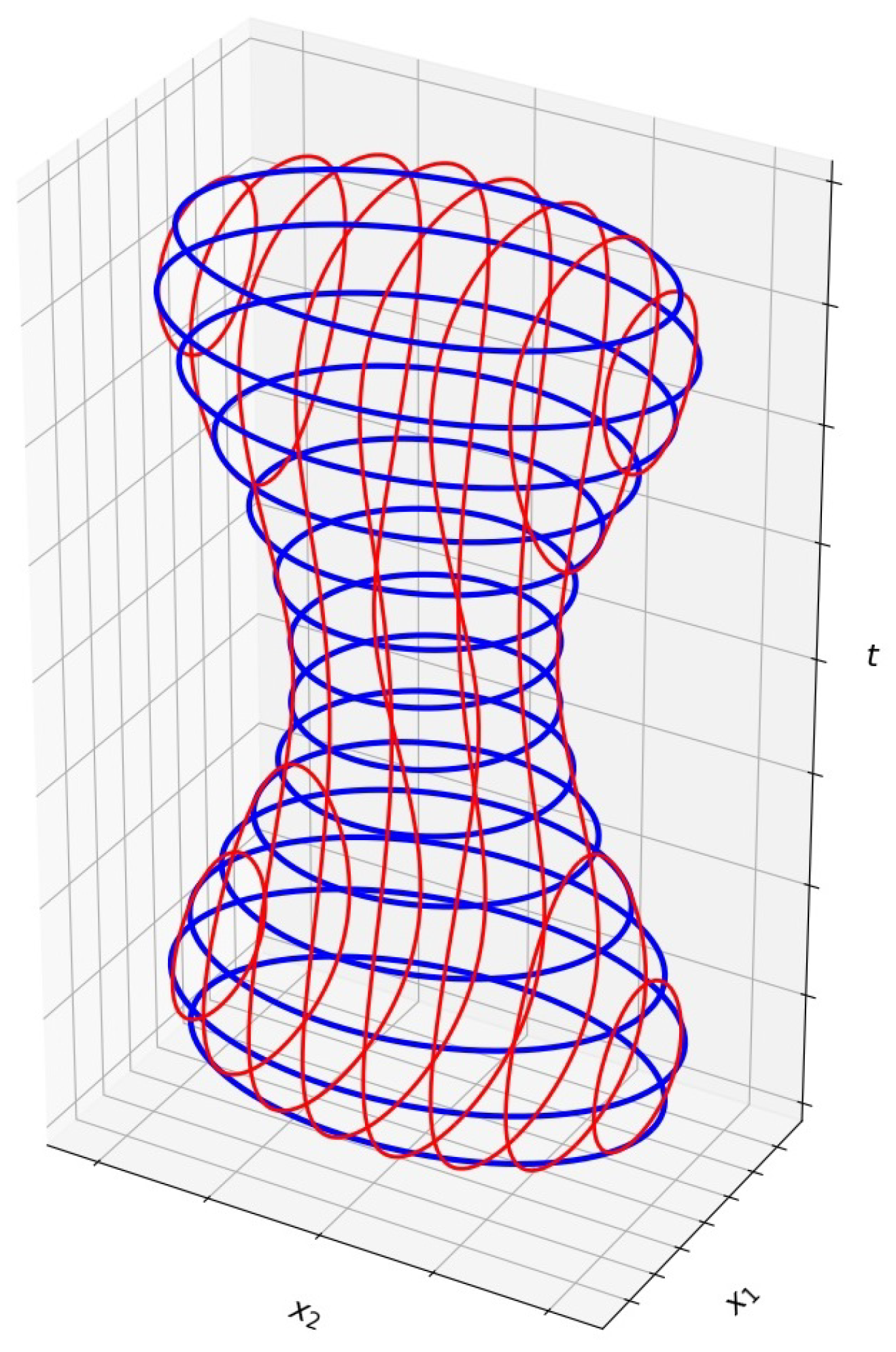
Figure 1 illustrates the challenges near tangency points. The figure depicts the graph of a continuous function $F:[0,1]\to K\left({[0,1]}^2\right)$, with smooth boundaries. The blue curves represent the boundaries of the given samples of F. The lowermost and uppermost points of the graph correspond to tangency points. As evident from the figure, the given samples do not provide sufficient information over a large neighborhood of these points. Typically, if the spacing between the given samples is h, the size of these neighborhoods is $O\left(h^{0.5}\right)$.

Figure 1. An example ($d=2$) of $Graph\left(F\right)$ and the given samples (in blue).

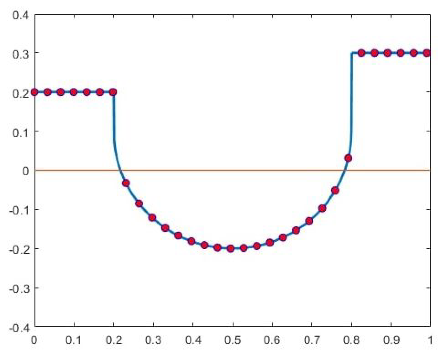
Another way to approach the problem is by examining the behavior of the signed-distance function near tangency points, offering deeper insight into a potential solution. Figure 2 illustrates this concept with the graph of a 2D set-valued function F, depicting a yellow ellipsoid containing a blue ellipsoidal hole. The planes $t=0.2$ and $t=0.8$ are tangent to the lower and upper boundaries of the hole, respectively. These parameter values also mark points where the topology of $F\left(t\right)$ changes: for $0<t\le 0.2$ and $0.8\le t<1$, $F\left(t\right)$ is a disc, whereas for $0.2<t<0.8$, $F\left(t\right)$ forms an annulus. Relevant to this specific case, Figure 3 presents the graph of the signed-distance function, $D(t;x^{\ast })$ as a function of t, for an $x^{\ast }$ near the hole. The function exhibits singularities at $t=0.2$ and $t=0.8$, characterized by the forms

$$\sim C_1{(t-0.2)}_{+}^{0.5},\mathrm{a}nd\sim C_2{(0.8-t)}_{+}^{0.5}.$$

Such singularities typically occur in the signed-distance function near smooth holes in $Graph\left(F\right)$. The circles in the graph represent the given data points, and the objective is to approximate the intersection of the graph with the line $y=0$ without prior knowledge of the location or nature of the singularities. Additionally, the figure reveals that the density of data points along the graph decreases as we approach the singular points. This specific example serves as a reference while presenting our proposed solution to the problem.

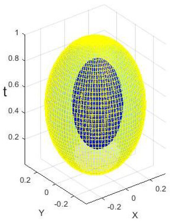
Figure 2. An example ($d=2$) of $Graph\left(F\right)$ - Ellipsoid with an ellipsoidal hole.

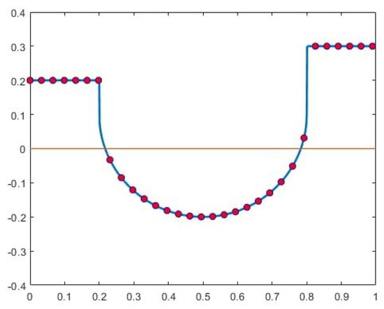
Figure 3. A typical signed-distance function $D(t;x^{\ast })$ with singularities.

3.2. High-Order Approximation of Singular Signed-Distance Functions

We now describe the algorithm for approximating the function $D(t;x^{\ast })$, as shown in Figure 3. Our approach is based on the method presented in [13], adapted to suit our specific needs.

1.

Deriving the signature of the singularities

We begin by applying a p-degree quasi-interpolation operator (see Section 2.3) to the given data ${\left\{D_i\left(x^{\ast }\right)\right\}}_{i=0}^N$ (represented by the circles in Figure 3). To facilitate this process, we extend the values ${\left\{D_i\left(x^{\ast }\right)\right\}}_{i=0}^N$ to the left and right by padding with zero values.

$$Q_{k-1}\left(D\right)\left(t\right)=\sum _{n\in \mathbb{Z}}{L}_{k-1}\left(D_{n,k}\left(x^{\ast }\right)\right)B_{k-1}\left({\displaystyle \frac{t}{h}}-n\right).$$

(7)

Next, we compute the errors in the quasi-interpolation approximation at the given data points:

$$E_i\left(D\right)=D_i\left(x^{\ast }\right)-Q_{k-1}\left(D\right)\left(ih\right).$$

(8)

We recall that the quasi-interpolation operator is a local operator, utilizing only a finite number of data points for each t. It provides an $O\left(h^k\right)$ approximation order to $C^k$ functions. Consequently, the errors $\left\{E_i\left(D\right)\right\}$ remain small at points where the signed-distance function is smooth but become significantly larger near the singular points $0.2$ and $0.8$. Additionally, large errors appear near the boundary points $t=0$ and $t=1$. For our application, we focus on the neighborhood of the singular points and disregard the large errors near the boundaries. We refer to the values $\left\{E_i\left(D\right)\right\}$ as ‘the signature of $D(t;x^{\ast })$’. For instance, the signature of the function in Figure 3 (with $k=4$) is illustrated in Figure 4.

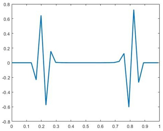Figure 4. An example of the signature of $D(t;x^{\ast })$ with singularities.

2.

Using the signature to identify singularity parameters

The next step, following [13], is to identify a singular function $\sigma$ whose signature closely matches that of $D(t;x^{\ast })$. As observed in Figure 4, for sufficiently small h, the effects of different singularities are well separated and can be analyzed independently.

In our case, while the exact locations of the singularities are unknown, their type is known. To address the left singularity in the given example, we fit a singular function of the form

$$\sigma \left(t\right)=\sum _{j=0}^q{a}_j{(t-s)}_{+}^{{\displaystyle \frac{j}{2}}}.$$

(9)

The unknown singularity location s along with the unknown coefficients $\left\{a_j\right\}$ are determined by performing ${\mathit{\ell }}_2$ minimization of the difference between the signature of $D(t;x^{\ast })$ and $\sigma \left(t\right)$, i.e.,

$$\{s^{\ast },\left\{a_j^{\ast }\right\}\}={\mathrm{argmin}}_{\{\{s,\left\{a_j\right\}\}}\left(\sum _{i=I_1}^{I_2}{(E_i\left(D\right)-E_i\left(\sigma \right))}^2\right),$$

(10)

where the indices $I_1$ and $I_2$ specify the interval of high signature corresponding to the left singularity. The operator $E_i\left(\sigma \right)$ computes the error of the quasi-interpolation approximation $Q_{k-1}\left(\sigma \right)$ at $t=ih$. The parameter q is chosen as $q=2(k-1)$ to achieve the highest possible approximation order. We denote the resulting optimal parameters as $s^{\ast }$, ${\left\{a_j^{\ast }\right\}}_{j=1}^q$.

As proved in [13], the resulting singularity parameters approximate the exact singularity parameters with a high order of accuracy. In particular, the singularity location satisfies $|s-s^{\ast }|=O\left(h^k\right)$ as $h\to 0$.

3.

The ‘corrected approximation’ framework.

We can now construct the desired approximation of $D(t;x^{\ast })$ with the above singularity information. This process is performed locally, relying upon the locality property of the quasi-interpolation operator $Q_{k-1}$.

First, we apply $Q_{k-1}$ to the smoothed data $\{D_i\left(x^{\ast }\right)-{\sigma }^{\ast }\left(ih\right)\}$, where

$${\sigma }^{\ast }\left(t\right)=\sum _{j=0}^{2p}{a}_j^{\ast }{(t-s^{\ast })}_{+}^{j/2}.$$

(11)

This yields the smooth-part approximation $Q_{k-1}(D(·,x^{\ast })-{\sigma }^{\ast })\left(t\right)$. Following [13], the final approximation is obtained by correcting the smooth-part approximation by reintroducing the singular component:

$$\tilde{D}(t;x^{\ast })\equiv Q_{k-1}(D(·,x^{\ast })-{\sigma }^{\ast })\left(t\right)+{\sigma }^{\ast }\left(t\right).$$

(12)

Using the error estimates from [13], we obtain

$$|\tilde{D}(t;x^{\ast })-D(t,x^{\ast })|=O\left(h^k\right),\mathrm{a}sh\to 0.$$

(13)

4.

Computational aspects

The optimization problem in (10) is linear in the unknown coefficients $\left\{a_j\right\}$ but non-linear in the singularity location s. However, since $s^{\ast }$ is an approximation of one of the values $t_j^{\ast }$ where a tangent plane $t=t_j^{\ast }$ is tangent to $\partial \Omega$, and given that there are only a finite number of such values, much of the computational effort involved in solving the nonlinear problem can be reduced. Specifically, once $t_j^{\ast }$ is well approximated for a particular point $x^{\ast }$, the same approximation $s^{\ast }\approx t_j^{\ast }$ can be used for all points in a neighborhood of $x^{\ast }$, significantly reducing the need for repeated nonlinear optimization.

In general, the singularity exponent is also unknown. However, the assumption that $\partial \Omega$ is smooth implies that, in non-degenerate cases, the singularity exponent is expected to be $1/2$. Nevertheless, other possible exponents, such as $1/3$ and $1/4$, should also be considered.

Remark 2

(Approximating the tangency point $(t_j^{\ast },x_j^{\ast })$). The parameters obtained in the approximation ${\sigma }^{\ast }$ can also be utilized to derive an estimate of the tangency point $(t_j^{\ast },x_j^{\ast })$. Specifically, the value $|a_0^{\ast }|$ serves as an approximation of the distance between $x_j^{\ast }$ and $x^{\ast }$. Additionally, recall that computing each distance $D_i\left(x^{\ast }\right)$ involves determining the direction to the nearest point on the boundary. Let ${\overrightarrow{e}}_i$ be the direction associated with $D_i\left(x^{\ast }\right)$, where $ih$ is the closest point to s satisfying $ih\ge s$. Then, the approximation of $x_j^{\ast }$ is given by

$${\tilde{x}}_j^{\ast }\sim x^{\ast }+a_0^{\ast }{\overrightarrow{e}}_i.$$

While the approximation $t_j^{\ast }\sim s^{\ast }$ achieves approximation order $O\left(h^k\right)$, the approximation of $x_j^{\ast }$ is of order $O\left(h\right)$.

3.3. The Improved DFI Approximation

In Section 2.1, the function $D(t;x)$ is approximated by interpolating the data $\left\{D_i\left(x\right)\right\}$, resulting in the approximation $I(t;x)$. However, the new approach deviates from interpolation. Similarly to the original DFI method, instead of using Equation (2), we define the improved approximation of the set $F\left(t\right)$ by the set

$$\tilde{F}\left(t\right)\equiv \{x:\tilde{D}(t;x)\ge 0\}.$$

(14)

With this improvement, the approximation results established in Theorem 1 are now enhanced as follows.

Theorem 2.

Let Ω be a closed $(d+1)$-dimensional domain whose boundary $\partial \Omega$ consists of a finite number of mutually disconnected hypersurfaces that are $C^k$-continuous. Suppose we use the quasi-interpolation method using the operator $Q_{k-1}$ to obtain the approximation $\tilde{D}(t;x)$. For each $h>0$, consider any point $(t^h,x^h)$ where the reconstructed set $\tilde{F}\left(t^h\right)$ disagrees with the true set $F\left(t^h\right)$, i.e.,

$$x^h\in F\left(t^h\right)\cap \tilde{F}{\left(t^h\right)}^{c}or{x}^h\in F{\left(t^h\right)}^c\cap \tilde{F}\left(t^h\right).$$

(15)

Then, the distance from $(t^h,x^h)$ to the boundary $\partial \Omega$ satisfies

$$dist((t^h,x^h),\partial \Omega )=O\left(h^k\right),\mathrm{a}sh\to 0.$$

Proof. 

If the plane $t=t_h$ is not close to a plane that is locally tangent to $\partial \Omega$, the result follows from [1], as stated in Theorem 1 above. Assume now that the plane $t=s$ is tangent to $\partial \Omega$ at the point $(s,x_s)$. Without loss of generality, suppose the singularity in the signed-distance function near the tangency point has the form given in (9). Using the algorithms in Section 3.2, we obtain an approximation $s^{\ast }\approx s$. If $t_h$ lies between s and $s^{\ast }$, the result follows from the earlier observation that $\parallel s-s^{\ast }\parallel =O\left(h^k\right)$ as $h\to 0$, along with the assumption that $\partial \Omega$ is $C^k$-smooth.

The challenging situation is when $t_h>\max \{s,s^{\ast }\}$ and $x^h$ is near $x_s$. For a point of disagreement $(t^h,x^h)$ as defined in (15), it follows that $D(t^h,x^h)$ and $\tilde{D}(t^h,x^h)$ have opposite signs. Applying the error estimate (13), we conclude that $D(t^h,x^h)=O\left(h^k\right)$ as $h\to 0$. The proof follows by noting that

$$dist((t^h,x^h),\partial \Omega )\le D(t^h,x^h).$$

□

4. Building Implicit Approximation of $\mathbf{\partial }\mathbf{\Omega }$

4.1. Implicit Approximation of Smooth Curves and Hypersurfaces

When approximating a set with smooth boundaries, a natural and constructive approach is to approximate its boundaries directly. An effective method, applicable in any dimension, is to use an implicit representation. Specifically, the approximation of a $(d-1)$-dimensional hypersurface in ${\mathbb{R}}^d$ is defined as the zero-level set of a function $S:{\mathbb{R}}^d\to \mathbb{R}$. A key insight in this context is the following curve approximation result, as presented in [10].

Proposition 1.

Assume Γ is a $C^4$-smooth curve in ${[0,1]}^2$ with a minimal curvature radius greater than R. Furthermore, suppose its R-neighborhood is neither self-intersecting nor intersecting the boundaries of ${[0,1]}^2$. Let P be a square mesh of points in ${[0,1]}^2$ with mesh size $\delta <R/10$. The curve Γ subdivides ${[0,1]}^2$ into two domains, ${\Omega }_1$ and ${\Omega }_2$, thereby partitioning the mesh points P into two corresponding subsets, $P_1$ and $P_2$. We assign signed-distance values to the mesh points P as follows:

$$D\left(q\right)=dist(q,\Gamma ),q\in P_1,$$

$$D\left(q\right)=-dist(q,\Gamma ),q\in P_2.$$

Let $Q_3$ be the quasi-interpolation operator that maps vectors of values on P to the space of bi-cubic splines on ${[0,1]}^2$. Define $S_{ϵ}$ as the bi-cubic spline obtained by applying $Q_3$ to a perturbed signed-distance dataset

$$\tilde{D}\left(q\right)=D\left(q\right)+{ϵ}_q,\left|{ϵ}_q\right|\le ϵ.$$

Let ${\Gamma }_{ϵ}$ be the zero-level curve of $S_{ϵ}$. Then, the Hausdorff distance between Γ and ${\Gamma }_{ϵ}$ satisfies

$$d_{Haus}(\Gamma ,{\Gamma }_{ϵ})\le C_0{\delta }^4+\parallel Q_3\parallel ϵ.$$

(16)

The above result can be naturally extended to higher dimensions and higher-order approximations as follows.

Proposition 2.

Assume Γ is a $C^m$-smooth hypersurface in ${[0,1]}^d$ with a minimal curvature radius greater than R. Furthermore, suppose that the R-neighborhood of Γ is not self-intersecting and is not intersecting the boundaries of ${[0,1]}^d$. Let P be a square mesh of points in ${[0,1]}^d$, with mesh size $\delta <R/2m$. The hypersurface Γ subdivides ${[0,1]}^d$ into two domains ${\Omega }_1$ and ${\Omega }_2$, thereby partitioning the mesh points P into two corresponding subsets, $P_1$ and $P_2$. We assign signed-distance values to the mesh points P as follows:

$$D\left(q\right)=dist(q,\Gamma ),q\in P_1,$$

$$D\left(q\right)=-dist(q,\Gamma ),q\in P_2.$$

Consider $Q_{m-1}$ to be the quasi-interpolation operator mapping vectors of values on P to the space of $(m-1)$-order tensor product splines on ${[0,1]}^d$. Let $S_{ϵ}$ be the $(m-1)$-order tensor product spline defined by applying $Q_{m-1}$ to a perturbed signed-distance data

$$\tilde{D}\left(q\right)=D\left(q\right)+{ϵ}_q,\left|{ϵ}_q\right|\le ϵ,$$

and let ${\Gamma }_{ϵ}$ be the zero-level hypersurface of $S_{ϵ}$. Then,

$$d_{Haus}(\Gamma ,{\Gamma }_{ϵ})\le C{\delta }^m+\parallel Q_{m-1}\parallel ϵ.$$

(17)

4.2. Estimating the Distance of a Point from a Hypersurface

To compute distances from a hypersurface $\Gamma$, we propose using the projection procedure introduced in [12] and later extended to manifolds in [14].

Given a set of points X on an unknown hypersurface $\Gamma$ and a query point p near $\Gamma$, the procedure identifies a local reference plane and projects p onto a point $\Pi \left(p\right)$ near the hypersurface. This projection is computed through a local least-squares fit using a polynomial patch $T_p$. The distance $\parallel p-\Pi \left(p\right)\parallel$, or the Euclidean distance $|p-\Pi (p\left)\right|$, serves as a second-order approximation of $dist(p,\Gamma )$. A higher approximation order of $dist(p,\Gamma )$ can be obtained by evaluating $dist(p,T_p)$. The approximation order depends on the smoothness of $\Gamma$, the fill-distance of the set X, and the degree of the local polynomial approximation. A precise formulation of this relationship is provided below.

Definition 1

(Fill-distance). The fill-distance of a set of points X with respect to a hypersurface (or manifold) Γ is defined as the diameter of the largest open ball centered at a point on Γ that does not contain any point of X.

Proposition 3.

Let Γ be a $C^k$ d-dimensional hypersurface, and let X be a set of points on Γ with fill-distance $O\left(h\right)$. Consider a point p near Γ. Let $T_p$ be the local polynomial patch defined by the projection procedure in [14], with total degree $k-1$. Then, the distance from p to Γ satisfies

$$dist(p,\Gamma )=dist(p,T_p)+O\left(h^k\right),\mathit{as}h\to 0.$$

(18)

The proof follows from the approximation properties of local moving least-squares, as outlined in [11].

4.3. Distributing Points near $\mathbf{\partial }\mathbf{\Omega }$

To generate the implicit function representation, we adopt the approach outlined in [9]. In the first step, we distribute a set of points, denoted as $Q_h$, around the boundaries of the body, ensuring that they remain at a small, controlled distance from the boundary. These points must be densely distributed near the boundaries of the object to guarantee a high-quality approximation of the signed-distance function.

The primary source of points comes from the boundary of the given samples. These points are distributed along the boundaries of the given sets ${F\left(ih\right)}_{i=0}^N$, with a fill-distance of approximately h relative to the boundaries. We denote this collection of points as $Q_h^0$. It is important to note that this collection is not unique; the method of selecting the points depends on the representation of the given samples.

On its own, $Q_h^0$ is not sufficient for providing an efficient approximation of the boundary of F. Specifically, these points do not adequately cover regions of the boundary $\Gamma$ of $Graph\left(F\right)$, particularly near points where the boundary is tangent to the plane $t=\mathrm{constant}$. This limitation is clearly illustrated in the upper and lower sections of the boundary in Figure 1.

To ensure complete coverage of the boundary of $Graph\left(F\right)$, we propose two approaches outlined below.

4.4. Completion of $Q_h$ near Tangency Points

We propose two methods for adding the missing information near the tangency points. Both methods utilize the local singularity expansion defined in Section 3.2, with parameters specified by (10). We assume that a good approximation of the tangency points $(s_j^{\ast },{\tilde{x}}_j^{\ast })\sim (t_j^{\ast },x_j^{\ast })$ is already available, as described in Remark 2, for $1\le j\le J$.

First, we estimate the size of the neighborhood around $(t_j^{\ast },x_j^{\ast })$ where additional points need to be inserted. The size of this neighborhood is determined using the parameter $a_1^{\ast }$ in ${\sigma }^{\ast }$. A simple analysis shows that this neighborhood corresponds to a ball with radius $R_j={\left(a_{1,j}^{\ast }\right)}^2$. To define the missing points, we consider the set of points

$$X^{\ast }=\{x:x\in X_h\cap B({\tilde{x}}_j^{\ast },R_j)\},$$

(19)

where $X_h=\{(i_1,i_2,...,i_d)h,:(i_1,i_2,...,i_d)\in {\mathbb{Z}}^d\}$ and $B(x,R)$ is the closed ball of radius R centered at x.

For each $x^{\ast }\in X^{\ast }$, we apply the procedure outlined in Section 3 and find the zero of $\tilde{D}(t;x^{\ast })$, $t^{\ast }$. The point $q^{\ast }=(t^{\ast },x^{\ast })$ serves as an approximation of the intersection of the line $x=x^{\ast }$ in ${\mathbb{R}}^{d+1}$ with $\partial \Omega$. This process is repeated for all neighborhoods around the tangency points. The collection of all points $q^{\ast }$ forms the set of points $Q_h^{\ast }$, which, when combined with the points $Q_h^0$, constitutes the required set of points $Q_h$ for constructing the implicit function.

An alternative, computationally simpler approach to complete the points $Q_h^{\ast }$ is inspired by a similar technique used in [3] for the case $d=1$, and proceeds as follows.

We construct a local polynomial approximation $P_j^{\ast }\left(x\right)$ of the boundary of $\Omega$ near each tangency point. This polynomial is obtained by performing a local least-squares fitting to the points in $Q_h^0$ that are the closest to ${\tilde{x}}_j^{\ast }$. By using a polynomial of total degree $\le 2n-1$, we achieve a local approximation of order $O\left(h^n\right)$ to the boundary $\partial \Omega$. The points near $\partial \Omega$ are then computed as follows:

$$Q_{j,h}^{\ast }\equiv \{(P_j^{\ast }\left(x^{\ast }\right),x^{\ast }):x^{\ast }\in X^{\ast }\}.$$

(20)

We apply this construction to all neighborhoods of the tangency points, gathering the resulting points into the set

$$Q_h^{\ast }={\cup }_{j=1}^J{Q}_{j,h}^{\ast }.$$

We then redefine the complete set as

$$Q_h=Q_h^0\cup Q_h^{\ast }.$$

In both approaches, the points in $Q_h$ provide a well-approximated representation of $\partial \Omega$ while maintaining a fill-distance of order $O\left(h\right)$ with respect to $\partial \Omega$.

Remark 3

(Approximation orders of $Q_h^{\ast }$). Each of the algorithms described above generates points near $\partial \Omega$ with a specific approximation order $O\left(h^{\nu }\right)$ as $h\to 0$.

• In the first approach, according to Theorem 2, the approximation order is $\nu =k$, where k is the smoothness index of the boundary.
• For the second approach, $\nu =n$ where $2n-1$ is the degree of the polynomial used for the local approximation.

4.5. Building and Analyzing the Implicit Function Approximation

Our goal is to construct a tensor product cubic spline $S(x_1,x_2,...,x_{d+1})$, whose zero-level set provides the approximation to $\partial \Omega$. Following the approach in [10], we look for S, which is an approximation to the signed-distance function from $\Gamma =\partial \Omega$. To construct S, we first overlay a uniform (d+1)-dimensional grid of ${(N+1)}^{d+1}$ points P on the domain ${[0,1]}^{d+1}$.

Recalling that $h=1/N$, each point $p\in P$ lies on one of the given cross-sections ${\left\{F\left(ih\right)\right\}}_{i=0}^N$. This allows us to determine whether p is inside or outside $Graph\left(F\right)$. To each point p, we assign the value of its approximate distance from $\Gamma$, with a plus sign if it is inside $Graph\left(F\right)$ and a negative sign if it is outside.

For each point $p\in P$, we aim to approximate its distance from $\Gamma$ using the procedure outlined in Section 4.2. Instead of exact data on the boundary of $\Gamma$, we utilize the points $Q_h$, which are located at a distance $O\left(h^{\nu }\right)$ from $\Gamma$ (see Remark 3). By applying the projection approach from Proposition 3, and choosing a sufficiently high degree for the local polynomial approximation, we achieve distance estimations with an error of $O\left(h^{\nu }\right)$ as $h\to 0$.

Using the quasi-interpolation operators introduced in Section 2.3, we construct a bivariate spline S of degree m on a uniform grid with knot spacing $h=1/N$, using the signed-distance values collected at the points P.

We define the zero-level of the resulting spline S as $\tilde{\Gamma }$, which serves as the desired approximation of $\Gamma$. The following approximation result follows directly from Proposition 2.

Corollary 1.

Let the boundary $\Gamma =\partial \Omega$ satisfy the smoothness assumptions stated in Proposition 2. Suppose the approximated signed-distance values at the grid points P are defined as described above. Let S be the tensor product spline of degree m, constructed using quasi-interpolation applied to these approximated signed-distance values. Denoting the zero-level of S by $\tilde{\Gamma }$, we obtain the following error bound:

$$d_{Haus}(\partial \Omega ,\tilde{\Gamma })\le C_1{h}^{m+1}+C_2{h}^{\nu },$$

(21)

where ν is defined in Remark 3.

5. Summary

In this work, we introduce ideas and algorithms for the high-order approximation of d-dimensional set-valued functions. In particular, we improve the approximation results of [1], demonstrating that a high approximation rate can be achieved even near points of topological change.

References

- Levin, D. Multidimensional reconstruction by set-valued approximations. IMA J. Numer. Anal. 1986, 6, 173–184. [Google Scholar] [CrossRef]
- Cohen-Or, D.; Solomovic, A.; Levin, D. Three-dimensional distance field metamorphosis. ACM Trans. Graph. (TOG) 1998, 17, 116–141. [Google Scholar] [CrossRef]
- Dyn, N.; Levin, D.; Muzaffar, Q. Interpolation of set-valued functions. IMA J. Numer. Anal. 2024, drae031. [Google Scholar] [CrossRef]
- Dyn, N.; Farkhi, E.; Mokhov, A. Approximation of Set-Valued Functions: Adaptation of Classical Approximation Operators; Imperial College Press: London, UK, 2014. [Google Scholar]
- Barequet, G.; Shapiro, D.; Tal, A. Multilevel sensitive reconstruction of polyhedral surfaces from parallel slices. Vis. Comput. 2000, 16, 116–133. [Google Scholar] [CrossRef]
- Kels, S.; Dyn, N. Reconstruction of 3D objects from 2D cross-sections with the 4-point subdivision scheme adapted to sets. Comput. Graph. 2011, 35, 741–746. [Google Scholar] [CrossRef]
- Schumaker, L.L. Reconstruction of 3-D objects using splines. In Proceedings of the Curves and Surfaces in Computer Vision and Graphics, Santa Clara, CA, USA, 13–15 February 1990; Volume 1251. [Google Scholar]
- Dyn, N.; Levin, D. Approximation of Set-Valued Functions with images sets in Rd. arXiv 2025, arXiv:2501.14591. [Google Scholar]
- Amat, S.; Levin, D.; Ruiz-Alvárez, J.; Yáñez, D.F. Global and explicit approximation of piecewise-smooth two-dimensional functions from cell-average data. IMA J. Numer. Anal. 2023, 43, 2299–2319. [Google Scholar] [CrossRef]
- Amat, S.; Levin, D.; Ruiz-Álvarez, J. A two-stage approximation strategy for piecewise smooth functions in two and three dimensions. IMA J. Numer. Anal. 2022, 42, 3330–3359. [Google Scholar] [CrossRef]
- Levin, D. The approximation power of moving least-squares. Math. Comput. 1998, 67, 1517–1531. [Google Scholar] [CrossRef]
- Levin, D. Mesh-independent surface interpolation. In Geometric Modeling for Scientific Visualization; Springer: Berlin/Heidelberg, Germany, 2004. [Google Scholar]
- Lipman, Y.; Levin, D. Approximating piecewise-smooth functions. IMA J. Numer. Anal. 2010, 30, 1159–1183. [Google Scholar]
- Sober, B.; Levin, D. Manifold approximation by moving least-squares projection (MMLS). Constr. Approx. 2020, 52, 433–478. [Google Scholar]
- Dyn, N.; Farkhi, E.; Mokhov, A. Approximations of set-valued functions by metric linear operators. Constr. Approx. 2007, 25, 193–209. [Google Scholar] [CrossRef]
- Speleers, H. Hierarchical spline spaces: Quasi-interpolants and local approximation estimates. Adv. Comput. Math. 2017, 43, 235–255. [Google Scholar] [CrossRef]
Disclaimer/Publisher’s Note: The statements, opinions and data contained in all publications are solely those of the individual author(s) and contributor(s) and not of MDPI and/or the editor(s). MDPI and/or the editor(s) disclaim responsibility for any injury to people or property resulting from any ideas, methods, instructions or products referred to in the content. |
© 2025 by the author. Licensee MDPI, Basel, Switzerland. This article is an open access article distributed under the terms and conditions of the Creative Commons Attribution (CC BY) license (https://creativecommons.org/licenses/by/4.0/).