Abstract
The optimization of overhead hoist transport (OHT) systems in semiconductor manufacturing plays a crucial role in improving production efficiency. In this study, the development of a discrete event simulation model to analyze the physical and control characteristics of an OHT system is presented, focusing on building a modular simulation framework for evaluating operational strategies by applying various optimization techniques. Additionally, a step-by-step analysis is introduced to optimize OHT operation using the developed model. The simulation model is broadly divided into three parts according to their purposes. The physical system encompasses the physical entities such as the equipment and vehicles. The experimental frame comprises a generator, which triggers experiments, and a result analyzer. Finally, the system controller is structured hierarchically and consists of an upper layer, known as the manufacturing control system, and subordinate layers. The subordinate layers are modularly divided according to their roles and encompass a main controller responsible for OHT control and a scheduling agent manager for dispatching and routing based on SEMI commands. The proposed simulation model adopts a structure based on the discrete event systems specification (DEVS). Since the hierarchical system controller may face challenges such as computational overhead and adaptability issues in real-world implementation, the modular design based on DEVS is utilized to maintain independence between layers while ensuring a flexible system configuration. Through an exploratory analysis using the simulation model, we adopt a step-by-step approach to optimize the OHT operation. The optimal operation is achieved by identifying the optimal number of OHT units and pieces of equipment per manufacturing zone. The results of the exploratory analysis for the three scenarios validate the effectiveness of the proposed framework. Increasing the number of OHT units beyond 17 resulted in only a 0.08% reduction in lead time, confirming that 17 units is the optimal number. Additionally, by adjusting the amount of equipment based on their utilization rates, we found that reducing the amount of equipment from 12 to five in process E-1 and from seven to three in the OUT process did not degrade performance. The proposed simulation framework was thus validated as being effective in evaluating OHT operational efficiency and useful for analyzing key performance indicators such as OHT utilization rates. The proposed model and analysis method effectively model and optimize OHT systems in semiconductor manufacturing, contributing to improved production efficiency and reduced operational costs. Furthermore, this work can bridge the gap between theoretical modeling and practical complexities in semiconductor logistics.
Keywords:
semiconductor manufacturing; logistics optimization; discrete event simulation; DEVS formalism; overhead hoist transfer operation; exploratory analysis MSC:
90B06
1. Introduction
In semiconductor manufacturing, the integration of simulation technologies has recently emerged as a critical approach, significantly contributing to the efficient management and optimization of complex production processes [1]. Wafer fabrication involves a highly complex production system encompassing hundreds of repetitive tasks. The efficient operation of numerous pieces of equipment and vehicles is essential to ensure the accuracy and efficiency of production in repetitive operations [2,3]. As the simultaneous production of semiconductor chips escalates, automated material handling systems (AMHSs) become increasingly important for automatic wafer transportation [4,5]. In an AMHS, 25 wafers are typically stored in a lot, called a front-opening unified pod (FOUP), which is transported between processing equipment through an overhead hoist transport (OHT) system along guide rails attached to the ceiling. As AMHSs were designed to reduce the production time, the optimization of OHT operations has been widely studied [6,7,8,9].
Previous studies on AMHSs have focused on optimizing OHT operation using simulation-based analyses through manufacturing-dedicated simulation tools such as eM-Plant (plant simulation), AutoModTM, and FlexSim [8,10,11]. For Example, Lin et al. [12] conducted a what-if analysis of optimized combinations of four vehicle types in an AMHS and evaluated the manufacturing performance based on the number of vehicles from a physical viewpoint [13]. Although specific tools have enabled detailed analyses, they are computationally expensive and have complex architectures that include several unused functions. Moreover, conducting various what-if analyses in a short time is challenging [11,14,15]. Therefore, OHT systems have been described using statistical models such as queuing and Markov chains, but they have limitations in expressing and modifying the complexity (i.e., dynamics) of OHT systems [11]. While advanced optimization algorithms, such as the discrete whale optimization algorithm (DWOA) proposed to solve the low-carbon flexible job shop scheduling problem (FJSP), have shown promise in addressing complex scheduling problems, they also face challenges such as high computational demands and difficulties in adapting dynamic changes in real time [16]. To facilitate a what-if analysis for optimal operation, a model should be modified and redesigned according to the target scenario. Hence, for efficient simulation-based analysis of an OHT system, a simulation model that exclusively encompasses the functions pertinent to the analysis objectives must be developed [17,18]. In addition, a modular model that facilitates the modification of its physical and logical parts during development is necessary. An analysis method with evolutionary optimization of the OHT system is also desirable while reconstructing the model during analysis. A modular model can allow for partial modifications when expanding the evaluated scenario without requiring modifications to the entire system. Hence, diverse experiments can be conducted.
We propose an overall process for OHT systems including (1) the development of a discrete event simulation model for analyzing the physical and control characteristics of OHT systems and (2) a step-by-step analysis method for optimizing the OHT operation based on the developed model. The model allows for easy reconfiguration using the discrete event system specification (DEVS) formalism in a multistage semiconductor manufacturing environment [19,20]. Compared to the modeling methods applied for operational optimization in semiconductor manufacturing processes to date, the discrete event system specification (DEVS) formalism can compensate for the limitations faced in OHT operational optimization to date because the modeling and simulation engine classes are separated, which maximizes model reuse and facilitates model management and extension [21]. Furthermore, it is applicable not only to OHT operational optimization in semiconductor manufacturing processes to date but also to many complex optimization problems. Our proposed DEVS-based OHT simulation model is divided into a physical system, a system controller, and an experimental frame. The hierarchical system controller comprises an upper layer called the manufacturing control system (MCS) and lower layers, which are further modularly divided into a main controller for the OHT system and a scheduling agent (SA) manager for dispatching and routing based on SEMI commands. This hierarchical structure was designed to facilitate the modification of each model. We implemented the physical behavior and OHT system control of every vehicle in the DEVSim++ environment [22], which adopts the DEVS formalism and allows for discrete event systems to be modeled in the C++ programming language.
We conducted an exploratory analysis to incrementally optimize the number of OHT units and amount of equipment by categorizing step-by-step scenarios to optimize OHT operations using the implemented simulation model. Experimental evidence has confirmed that employing gradual optimization, like determining the optimal number of vehicles and pieces of equipment for an entire process, improves key performance indicators (KPIs). The results from one scenario revealed that the OHT utilization rate reached 98.47% when 17 units were employed. For two other scenarios, the KPIs were substantially improved by using three pieces of equipment in a specific zone.
In this study, we present a method for developing simulation models and demonstrate an exploratory analysis to identify the optimal number of OHT units and pieces of equipment through a data analysis of the simulation results. Compared with existing simulation frameworks, the proposed model adopts a lightweight modular structure, which reduces computational overhead and improves adaptability to real-time scenario changes. In addition, by integrating a hierarchical system controller with the DEVS-based modular design, the model enables independent adjustments at different control levels, improving the efficiency of the optimization process. The proposed modular model allows for easy modification of logical components during development and introduces an exploratory analytical method that optimizes the OHT unit and equipment operations through scenario expansion. The experimental results confirm that the proposed approach not only improves OHT utilization and equipment efficiency but also provides a flexible basis for future optimization of semiconductor manufacturing logistics. By applying this approach to various scenarios, rapid comparison and analysis of different algorithms in real-time operational environments can be performed, enabling flexible OHT scheduling and route optimization. This is expected to improve semiconductor manufacturing efficiency and to reduce operating costs.
The remainder of this article is organized as follows. Section 2 presents related work, and Section 3 details the proposed modeling and simulation (M&S) approach, including the model design and an exploratory analysis. Section 4 explains the experimental design to demonstrate the exploratory analysis proposed in this study. Section 5 presents the experimental results for a semiconductor manufacturing environment, and Section 6 presents a discussion of the findings. Finally, Section 7 provides our concluding remarks.
2. Related Work
Over the past few decades, most studies on AMHSs have focused on what-if analyses and simulation-based optimization from physics and control perspectives using M&S approaches, as listed in Table 1 [23,24,25].

Table 1.
Related research on AMHSs using the M&S approach.
Tool-based approaches often rely on plant simulations, such as eM-Plant developed by Siemens, owing to their embedded manufacturing libraries and built-in optimization functions. Lin et al. [12] conducted what-if analyses of both the optimized combinations of four vehicle types in an AMHS and manufacturing performance based on the number of vehicles from a physical viewpoint [13]. Regarding physical factors, AMHS routing has been applied to eM-Plant [26,27,28,29], and routing algorithms have been optimized [8,30].
The AutoModTM manufacturing simulator developed by Applied Materials has been used to analyze AMHSs. Nazzal and McGinnis [4] performed a simulation-based analysis of station utilization, that is, physical aspects in a 300 mm wafer factory. Furthermore, routing optimization using deep or machine learning has recently attracted considerable attention [2,9,31,32,33]. A general-purpose simulator with multiple degrees of freedom for simulation model development has also been used for AMHS analyses. Using the FlexSim simulator, Wang [5] analyzed the performance of an improved lot delivery time in 450 mm semiconductor manufacturing, and Wang et al. [10] and Chen et al. [34] analyzed the performance of AMHSs according to vehicle routing algorithms. Ben-Salem et al. [35] analyzed an AMHS by considering the number of vehicles and routing algorithm using the AnyLogic simulator.
Although current simulators reduce the time required to develop an AMHS model by providing a manufacturing library and graphical user interface, they often require long execution times. Liang and Wang [14] combined statistical models obtained from individual model execution results by constructing a modular AMHS simulation model to reduce the simulation execution time in eM-Plant. Although this approach shortened the simulation time, it failed to suitably represent the system dynamics.
To reflect the system dynamics, Mohammadi et al. [15] considered an AMHS as a queuing model in a MATLAB 2014 environment for method-based M&S. Subsequently, they performed an accuracy comparison with a simulation model developed using AutoModTM. Because a queueing model is abstract, its simulation characteristics are difficult to maintain. Therefore, Nazzal and McGinnis [4] and Wu et al. [11] constructed Markov chain models and compared their accuracy with that of the AutoModTM and eM-Plant simulation models, respectively.
Discrete event systems are more complex models than stochastic queueing models and have limitations in considering event characteristics because they must represent the processing of dynamically occurring events. To overcome this problem, AMHS simulation models have been constructed based on the DEVS formalism, which can express a representative model for a discrete event system. However, it is a simulation model for verifying the operation of physical assets in a cyber–physical system environment instead of an analytical model [36,37]. Similarly, Lee et al. [38] attempted to create an analytical model based on the DEVS formalism but could not analyze the results based on the implemented model.
Overall, although previous studies have attempted to reduce the simulation execution time, their results did not suitably reflect the system dynamics due to the underlying queuing and Markov chain models. However, our AMHS simulation model based on the DEVS formalism is useful when reproducing or analyzing complex dynamic systems as realistically as possible. In addition, studies that have included a DEVS structure with system dynamics did not support their empirical simulation results. Hence, we focused on constructing an AMHS simulation model based on the DEVS formalism and an analysis method for empirical simulation results to improve the operation of an OHT system.
3. Methods
A semiconductor fabrication plant, or fab for short, comprises various physical systems and can be modeled with a continuous discrete event system. Despite their complexity and logic, modeling approaches can differ depending on the simulation purpose. In purpose-oriented object-driven modeling, some characteristics should be abstracted. Hence, reconfigurable extensions of the simulator and a hierarchical structure should be considered for fab simulation. Accordingly, we developed a fab simulation based on the DEVS formalism to optimize the number of physical systems in the fab.
3.1. Proposed Process Approach
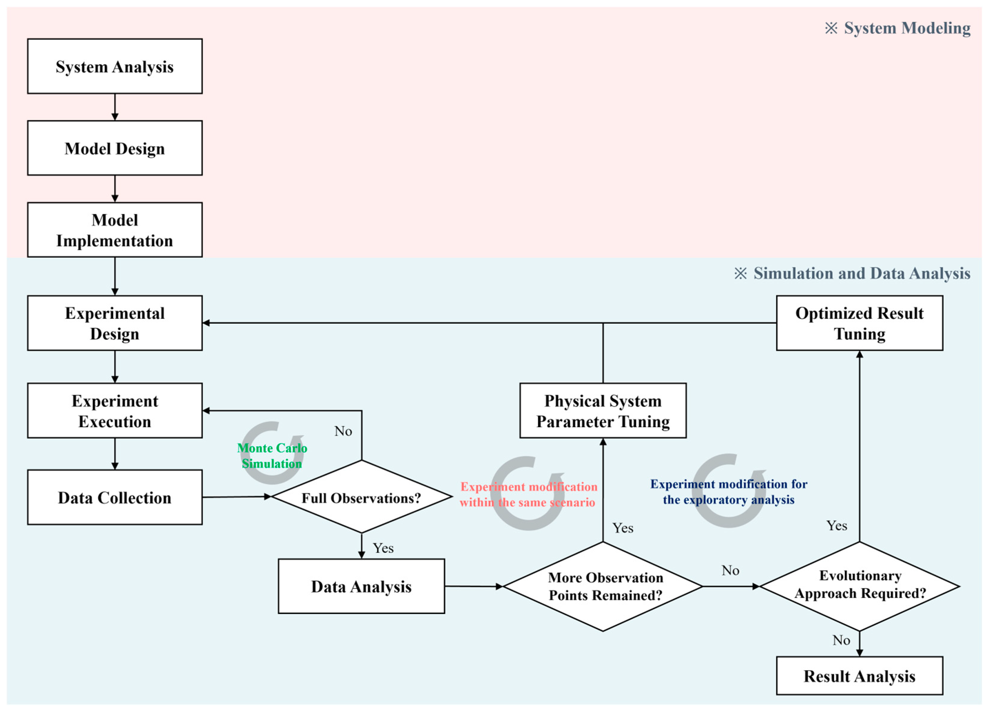
To develop the simulation model and analyze its results, we divided this study into two processes, as illustrated in Figure 1. The red-shaded region shows the process of target system analysis, modeling, and implementation. For modeling and result analysis, M&S approaches are often grouped, but we focused on both the development of the target system model and an exploratory analysis. Therefore, we divided the simulation (blue-shaded region) into three experimental phases. When the system is modeled (red-shaded region), the experimental design is determined and experiments are executed. For the statistical analysis, we repeated Monte Carlo simulations 20 times per case. With the full observations and their analyses, the second phase of the experimental modification was conducted for the same scenario, and the first phase was repeated. If no observations remained, the parameters from the previous scenario were tuned for the next scenario to perform an exploratory analysis. Finally, when the observations of all the scenarios were obtained, the results were analyzed.
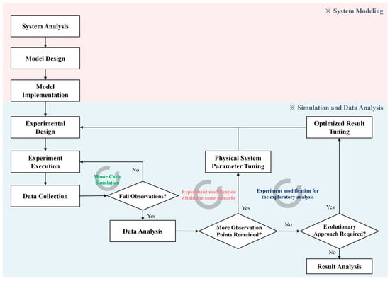
Figure 1.
Processes of target system M&S and exploratory analysis.
3.2. Overall System Architecture
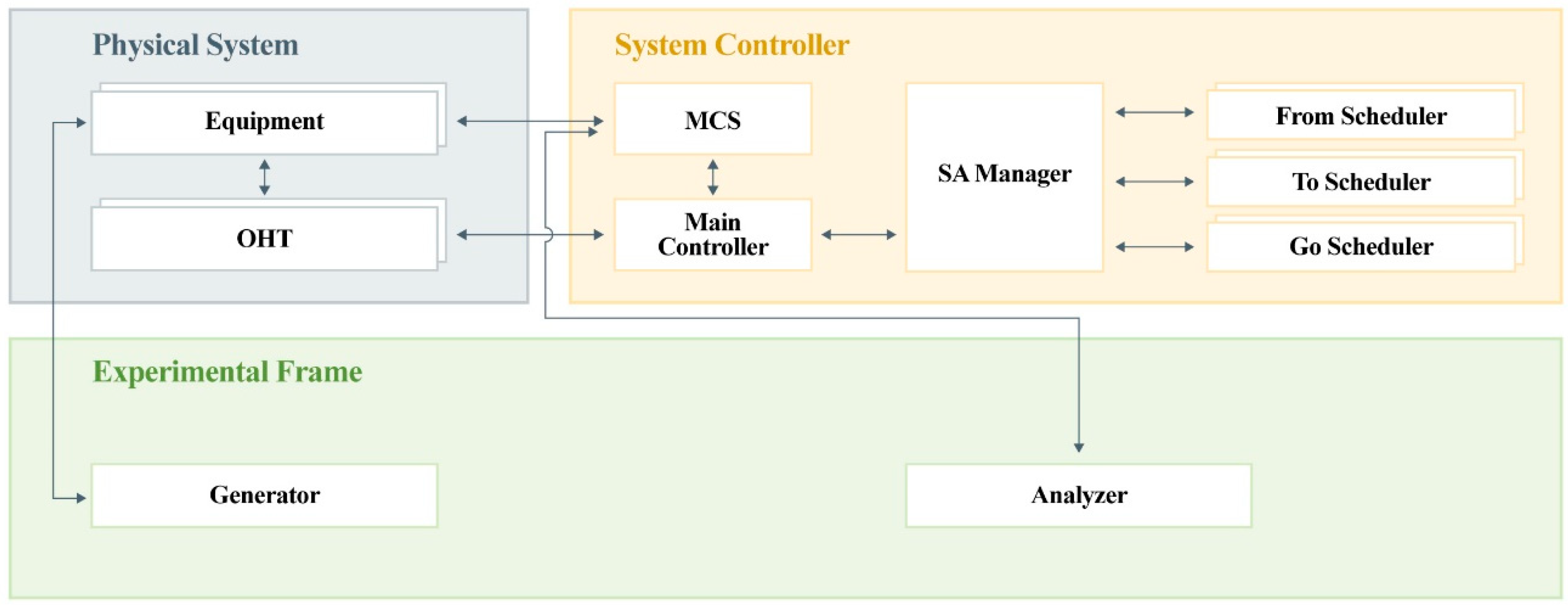
The proposed models were designed after analyzing the target system. The overall architecture of the proposed system is shown in Figure 2. The model consists of three parent systems: a physical system, a system controller, and an experimental frame.
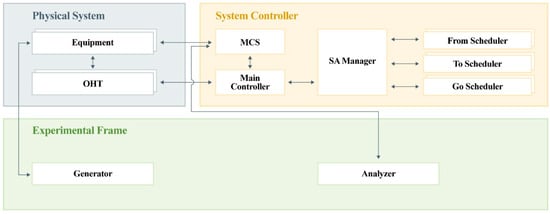
Figure 2.
Overall structure of proposed model.
The physical system is the parent system that performs actual tasks in the simulation and consists of the OHT system and processing equipment. The physical system generally receives commands from the system controller to perform actions. In practice, the OHT rail can also be considered part of the physical system, but we include it in the map configuration data instead because the equipment and the OHT unit interact under the designed models and their characteristics can be considered an active case. On the other hand, the rail can be considered a passive component that does not interact with any other model once loaded. Therefore, we include the rail in the map configuration and environmental data, such as the OHT specifications. The equipment specification and map configurations are written in JSON format and loaded via the generator model at the beginning of the simulation.
The system controller is the parent system that manages the physical system and material flow in the fab and consists of an MCS, a main controller, an SA manager, and schedulers. The MCS is the highest-level layer and monitors the completion of all processes and the status of the physical system. For simulation, the MCS sends a command of the from–to pair message to the main controller using its designed logic. The main controller mainly controls the operation of the physical system. When it receives commands from the MCS, the main controller sends a scheduling request to the SA manager. After the result is received, it sends a command to the OHT unit to proceed with production. The SA manager controls the schedules depending on the given command. Commands are identified as from, to, and go messages. For example, to load the complete FOUP from the equipment, a from command is given to an OHT unit. For the OHT unit to move to the next process and unload the FOUP, a to command is created as a pair with the from command. Finally, a go command is created to remove any blocking OHT unit in a congested region. Depending on the received command, the SA manager dynamically creates and removes schedulers. The main controller has three predefined parts: action commands, input/output ports, and a logic processor. The SA manager is divided into three message-processing parts.
The experimental frame is the parent system that is mainly responsible for starting the simulation and analyzing the results and is composed of a generator and an analyzer. The generator loads the environmental data and generates input jobs for the first process equipment to start operation. When the target simulation is complete, the analyzer receives the simulated information from the MCS and analyzes the KPIs.
3.3. Exploratory Analysis
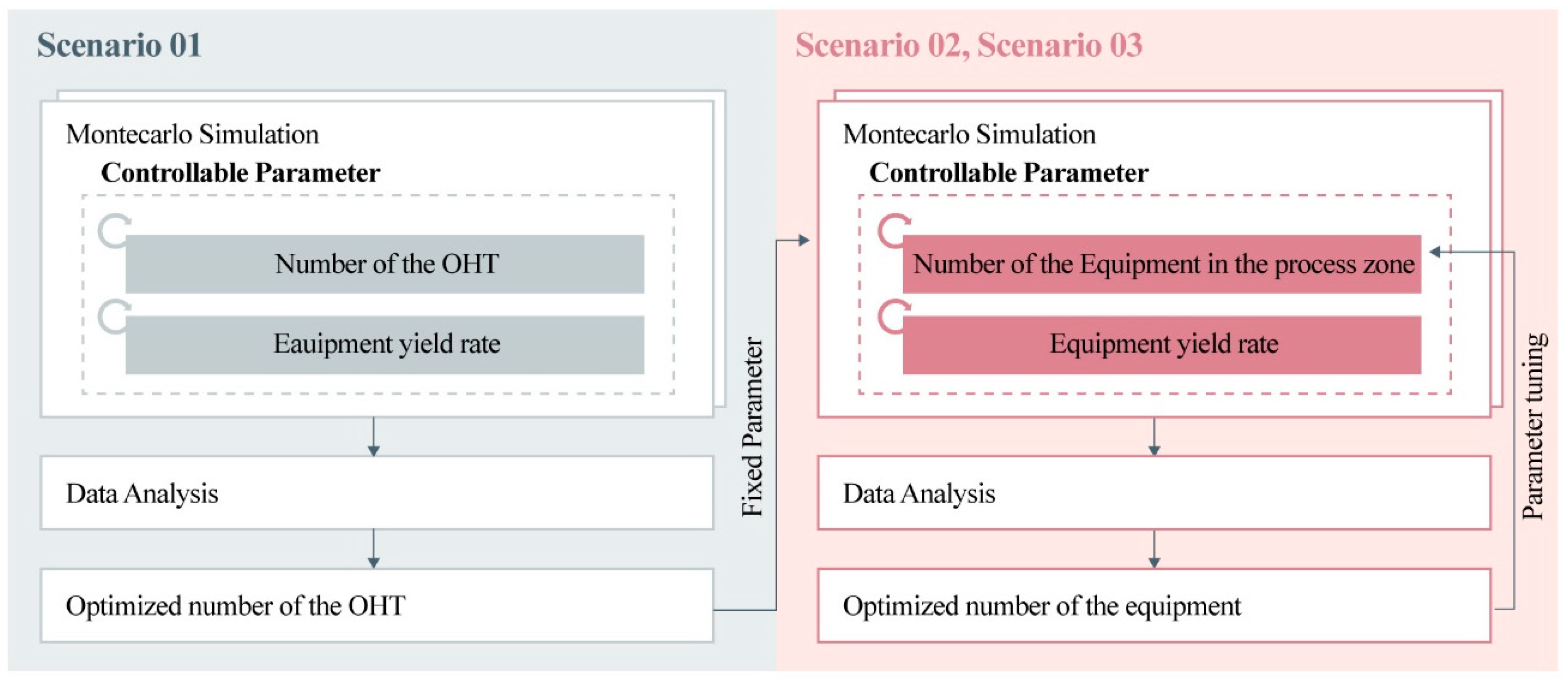
As illustrated in Figure 3, this exploratory analysis comprises three scenarios, all of which are based on a stepwise sensitivity analysis approach. The first scenario of the exploratory analysis, which we propose from a sensitivity analysis perspective, identifies how changes in OHT units affect key performance indicators (KPIs). Through this parametric sensitivity analysis, the optimal number of OHT units for all equipment yield rates was determined and reflected in the following scenarios. In the following two scenarios, we conducted exploratory sensitivity analysis to optimize the number of equipment in a specific process area. Scenario 2 focuses on optimizing the number of equipment in the most bottlenecked process area, while scenario 3 fixed the number of OHT units and equipment optimized in scenarios 1 and 2 to optimize the number of equipment in the second most bottlenecked process area. Detailed scenarios and case study results are discussed in Section 5.
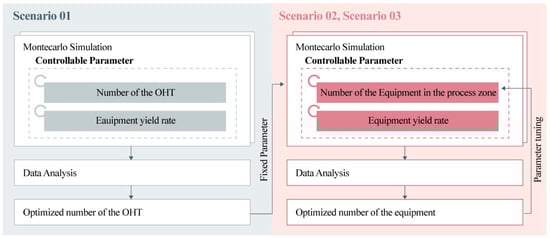
Figure 3.
Exploratory analysis scenarios.
3.4. Design of Modular Simulation Model
3.4.1. MCS
For fluent control of the materials in a fab, the overall process must be monitored, and decisions should be made automatically. Various baselines are available for the MCS to dispatch jobs, such as first-in first-out, the shortest processing time, and the shortest setup time [39]. We adopted a first-in first-out approach for job distribution. Command matching proceeded as follows. If a piece of equipment finished production, the MCS searched for the next equipment for the process and generated a from–to pair command to connect it with the OHT unit. This command specifies the departure equipment and the destination equipment for OHT. In other words, it provides routing instructions to ensure that the completed FOUP is smoothly transported to the appropriate next process. Each command is assigned a unique command identifier to specify its type. To match the equipment, the MCS first verifies the status of the physical system and then meets the FOUP specifications. If the FOUP quality is acceptable, the MCS matches the next regular process. In contrast, for low-quality results, a repair process is matched before the regular process. If all the physical systems are busy, the MCS stacks the message into the buffer and searches for the next message to match. If no matching message is found, the MCS waits and sends messages from the buffer after the OHT unit completes the transportation and is ready to receive a new task. For the data analysis, when the target FOUP is completed, the MCS sends information about its movement path and processing time to the analyzer.
3.4.2. Main Controller
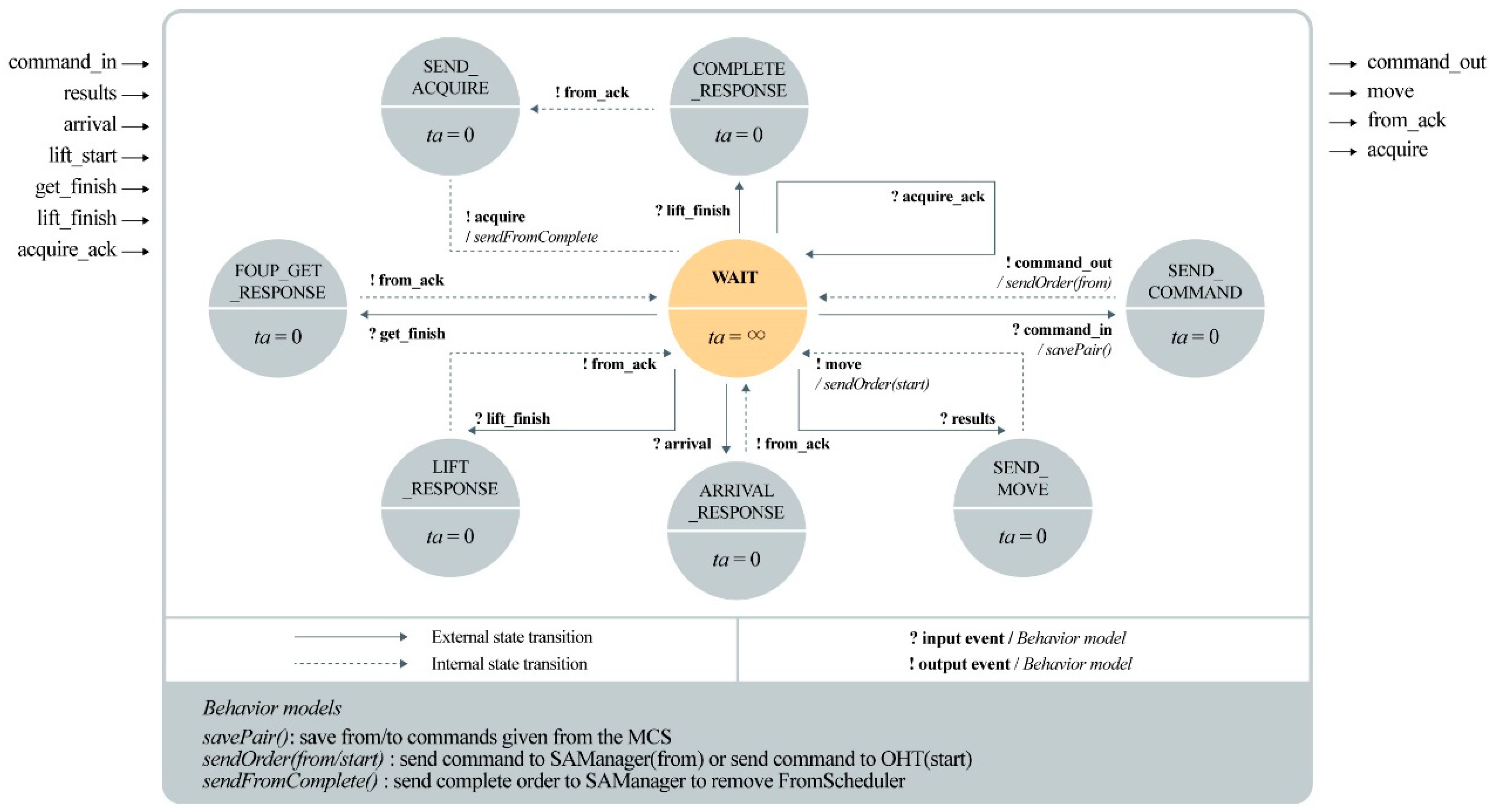
The main controller was designed to control the OHT system using commands from the MCS. Figure 4 presents the operation logic of a from message as a DEVS diagram. The left and right sides of the rectangle indicate the input and output ports. Inside the rectangle, the states, time advances, and behaviors of the OHT system are described. For example, the main controller begins in the WAIT state until a command is received. When it receives from–to pair commands from the MCS, it divides them into two separate commands for sequential discrete operation, and a transition occurs to state SEND_COMMAND. For the from process, the main controller sends a from request command to the SA manager as the output. After the OHT unit is allocated and scheduled, the main controller receives the scheduling results, sends a move command to the OHT unit, and interacts with each process. To automate the sequence, all time advances of the main controller are set to zero. When a requested from command is completed by the OHT unit, the main controller sends an acquire message to the SA manager to remove the tasks completed by the schedulers and a to command continues as the next process.
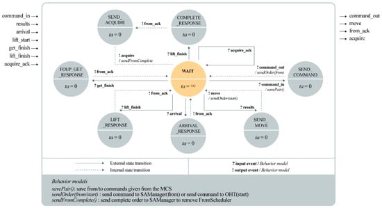
Figure 4.
Atomic DEVS model diagram of the main controller and the from message process.
The DEVS expressions are given in Equations (1)–(8). The dynamics of the atomic model in the DEVS formalism can be expressed using seven components, as shown in Equation (1), and its component logic is expressed in Equations (2)–(8). X and Y represent the input and output events, respectively; S represents the state set of the main controller; δext is an external transition function that changes states by inputting X; and δint is an internal transition function that changes the states according to its defined time advance TA, which is a function that indicates the time spent in a state. When an internal transition occurs, output function λ generates output Y.
3.4.3. SA Manager and Schedulers
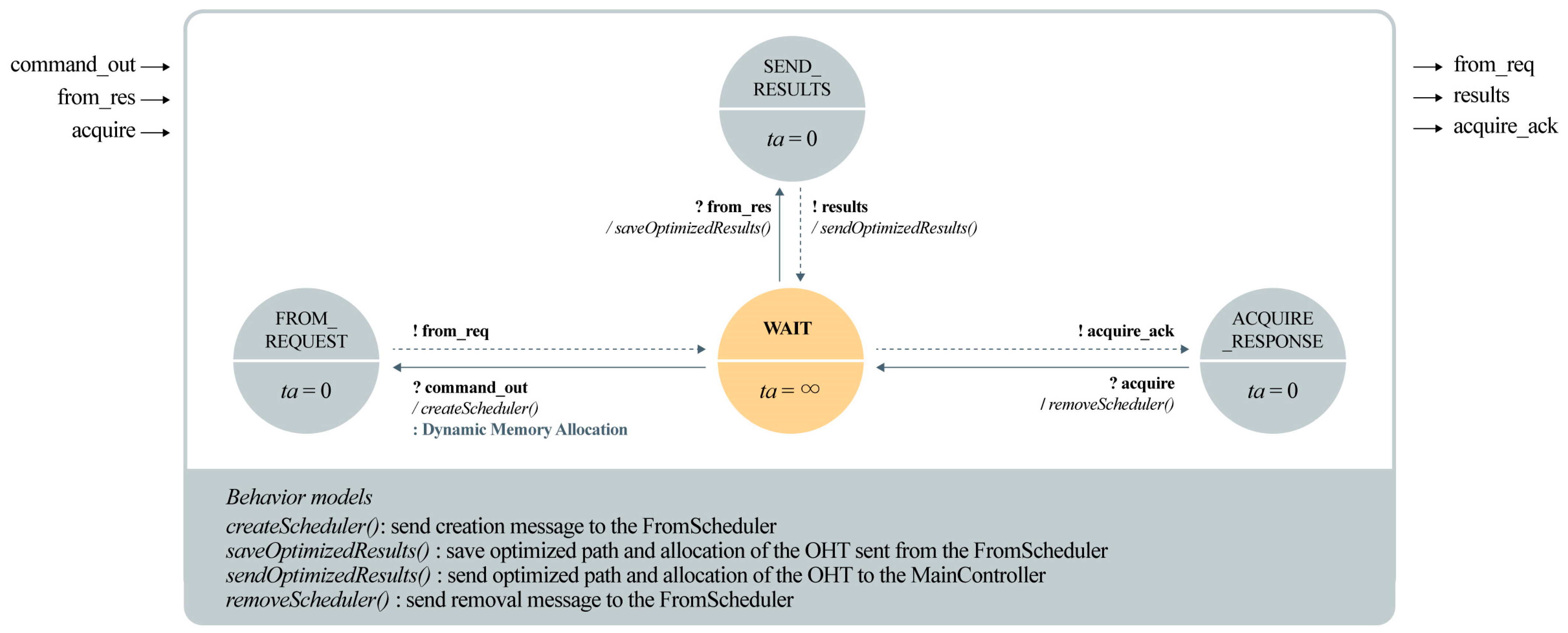
The SA manager controls the schedulers by receiving commands from the main controller and dynamically creates and removes schedulers according to the command requests. The from message process is depicted in Figure 5, and the DEVS expressions are described in Equations (9)–(16). When the SA manager receives an OHT and allocation command via the command_out input port, it transitions to the FROM_REQUEST state, creating a scheduler to handle the request. The scheduler then sends a transport request message. Once the OHT assignment and route optimization results are received via the from_res input port, the state transitions to SEND_RESULTS, forwarding the optimized result to the main controller. After the command is executed, the SA manager receives an acquire message, and the designated scheduler is removed. Although not shown in any figure or DEVS expression, if the from process is completed, a to scheduler is created for the unload operation of the OHT unit, which only schedules an optimized path because the unit is already allocated by the previous scheduler. If the scheduled path is blocked by another OHT unit, the to scheduler sends a NACK message to the SA manager, which in turn forwards the NACK message to the main controller to remove the blocking OHT unit. A go scheduler can be created to move the OHT unit away from the congested region if the scheduled commands are completed by the OHT unit.
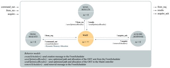
Figure 5.
Atomic DEVS model diagram of the SA manager and the from message process.
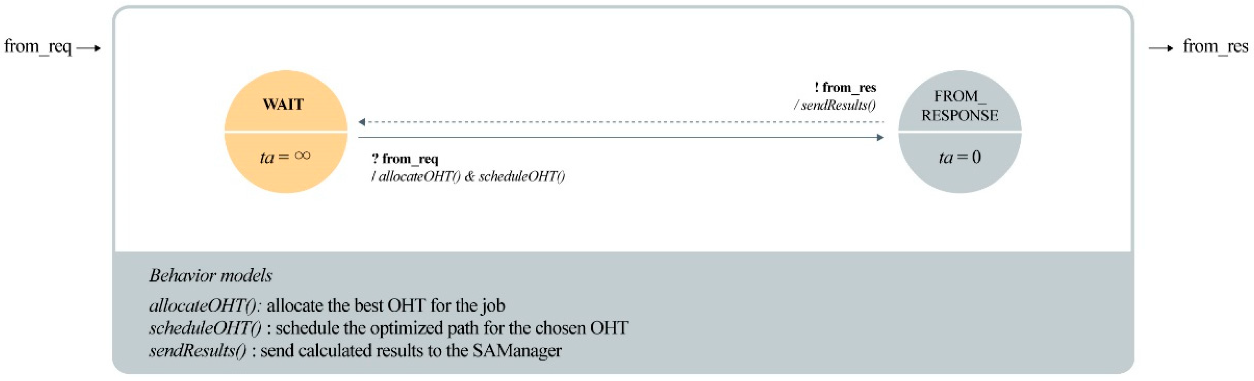
The scheduler mainly allocates and organizes the operations of OHT units according to received commands. Figure 6 presents a DEVS diagram of the from scheduler. The process is described in Equations (17)–(24). With the received request command, the from scheduler allocates the nearest OHT unit to the equipment, which is in an IDLE state, and determines the optimized path. The allocated and scheduled results are then sent to the SA manager. Because the simulation is experimented for a small-fab design, the execution time of the algorithm is not considered. In this study, the Dijkstra algorithm was used as an initial model for path search in the OHT system. Dijkstra guarantees an optimal path and can find the shortest path to all destinations in a single computation, making it stable even in complex network environments such as OHT. The A* algorithm can also be used for OHT path planning, but it is difficult to set up a suitable heuristic, and if it is inaccurate, it can reduce the efficiency of the search. Since the main purpose of this study is to verify the OHT framework, Dijkstra was chosen to minimize the influence of environmental variables and to ensure consistent experiments. Since Dijkstra searches for a path based only on the given weights without any heuristics, it can perform a more accurate performance comparison and analysis of the OHT framework. However, in environments where the system is extended or real-time performance is required, alternative methods such as the A* algorithm can be considered, which requires an appropriate heuristic design that reflects the characteristics of the OHT network.

Figure 6.
Atomic DEVS model diagram of a scheduler and the from message process.
3.4.4. Equipment
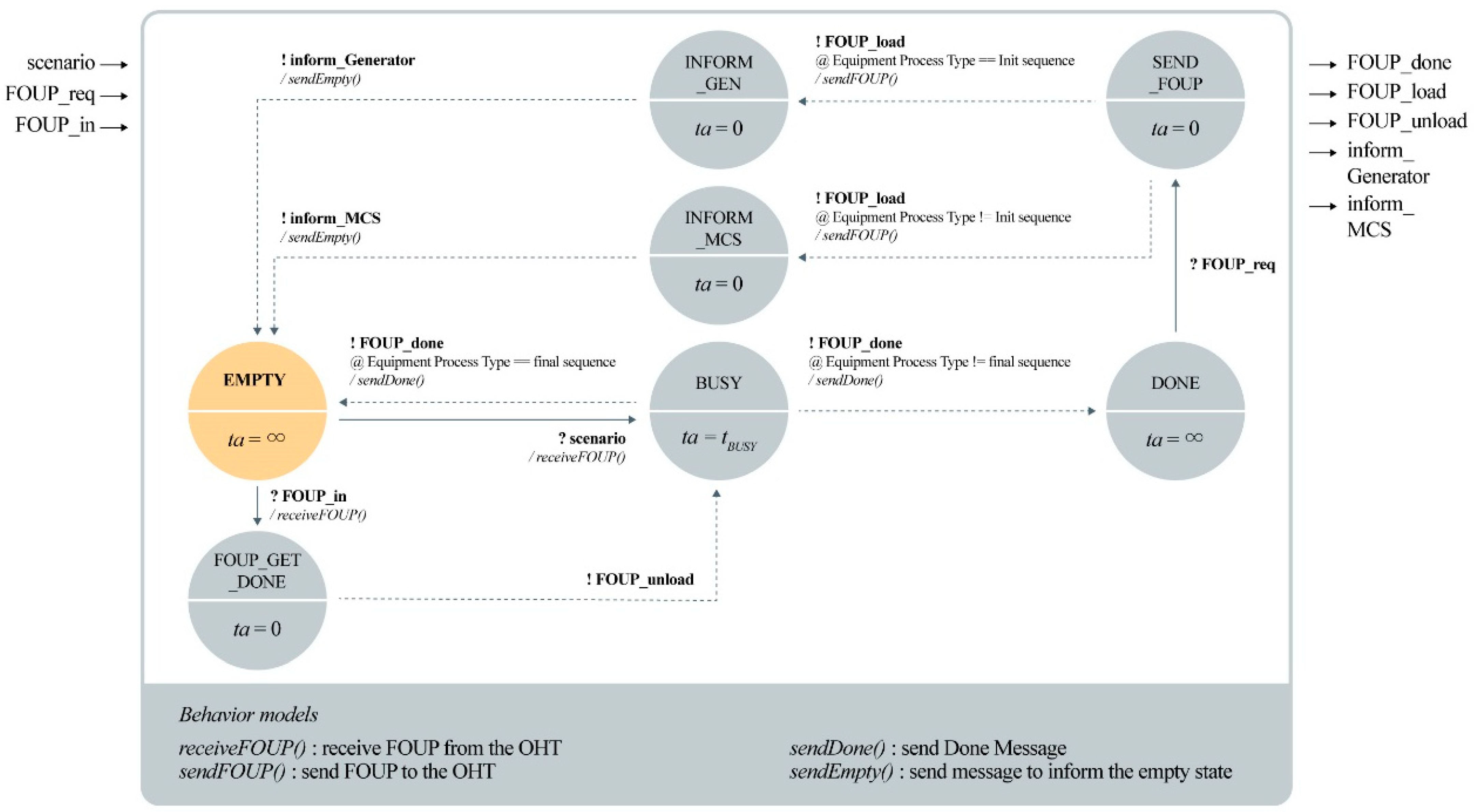
Semiconductor manufacturing can be divided into eight processes, and diverse types of equipment have been developed by various companies. Therefore, the form and specifications of different pieces of equipment may vary. For example, the input and output ports of equipment can either be separate or integrated into a bidirectional port. To obtain intuitive results for material flow, we consider equipment with one bidirectional port and assume similar specifications. This equipment logic is illustrated in Figure 7 and described in Equations (25)–(32). When the simulation engine starts, all the pieces of equipment are set to the EMPTY state and wait for a job to be processed. For the first piece of equipment to start a process, the corresponding scenario is received by the generator, and a transition to the BUSY state occurs. For the other pieces of equipment, FOUPs are received by the to command, and interactions with the OHT units occur. Upon FOUP arrival, a transition to the FOUP_GET_DONE state occurs, and the FOUP is unloaded from the OHT unit with the corresponding transition to the BUSY state. The processing time of a piece of equipment depends on the parameters encoded in the environmental data. At the end of production, the equipment transitions to the DONE state and sends a complete message to the MCS that initially requested the load operation.
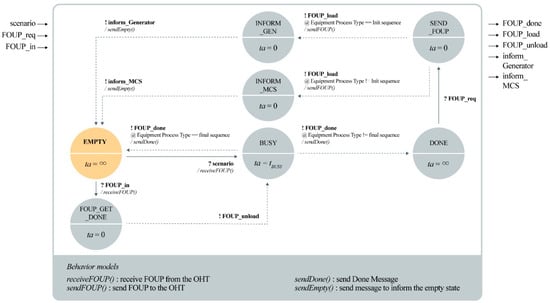
Figure 7.
Atomic DEVS model diagram of equipment.
If a piece of equipment handles the final sequence of material production, it returns to the EMPTY state, and the completed job of the final sequence is assumed to be carried out by a worker for quality assurance. Upon arrival of the OHT unit, the equipment unloads the FOUP and transitions to the SEND_FOUP state. If the equipment is handling the beginning of the sequence, it sends a message to the generator to continue the target job. Otherwise, it sends a message to the MCS about its EMPTY state so that the MCS can try to match another process.
3.4.5. OHT System
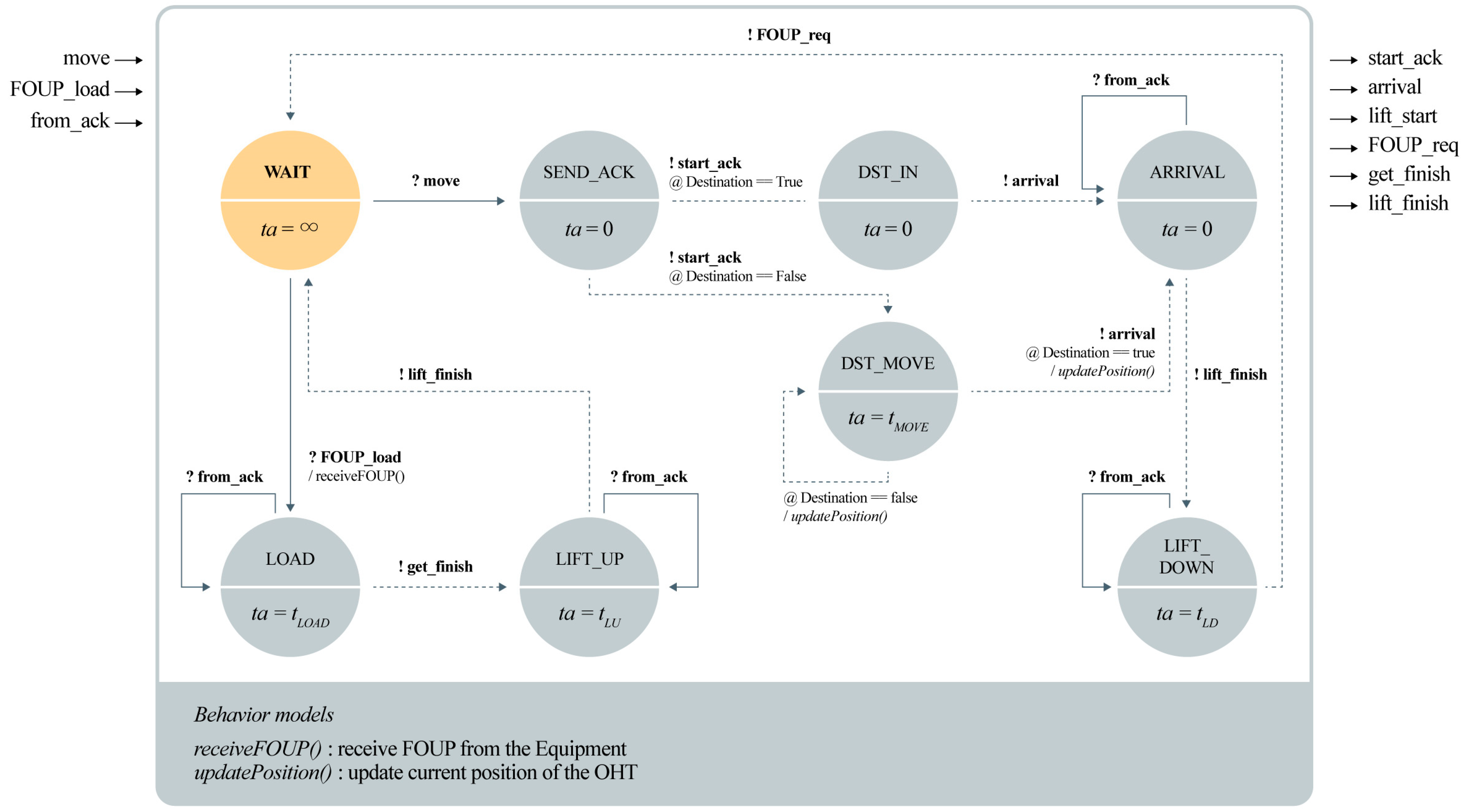
The main states of an OHT unit include move, arrival, lift down, load/unload, and lift up. The state transitions depend on the received command. Figure 8 and Equations (33)–(40) describe the logic of an OHT unit for the from message process, which indicates a load operation. At the beginning of the simulation, the OHT unit waits for commands in the WAIT state. When a move command is received, the OHT unit sends an ACK message to the main controller and moves to its destination. If the OHT unit is already at the destination, it transitions to the DST_IN state, sending an arrival message, indicating its transition to the ARRIVAL state. Otherwise, if the OHT unit is not at its destination, it transitions to the DST_MOVE state and starts moving according to the defined TA. When the OHT unit reaches a designated piece of equipment, it transitions to the LIFT_DOWN state, sends a FOUP request message to the equipment, and returns to the WAIT state. If the FOUP is received in the LOAD state, it transitions to the LIFT_UP state and lifts the loader. Subsequently, it sends a lift finish message to the main controller and returns to the WAIT state to receive its next command. Each physical operation is designed to interact with the main controller, and all the TA values of the states are contained in the environmental data, like equipment information.
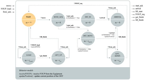
Figure 8.
Atomic DEVS model diagram of an OHT unit and the from message process.
3.4.6. Generator
For the KPI analysis, the starting point of the simulation must be defined. We introduce a generator to create jobs for the first process to begin. The generator is included in the experimental frame, and it also loads environmental data and generates target jobs. To create a job, the generator first checks the status of the equipment and pending target jobs. For example, if the equipment in the first process is in the EMPTY state and jobs remain, the generator sends a job to the equipment to initiate the process. Otherwise, the generator waits for an empty message to be received from the equipment.
3.4.7. Analyzer
The analyzer is also included in the experimental frame and used to analyze the simulation results. The MCS monitors job completion, and when the simulation is complete after accomplishing all the assigned tasks, the analyzer receives a completion message from the MCS to start analysis. In this study, we designed an analyzer to calculate five KPIs: production lead time, buffer wait time of FOUP, OHT utilization rate, go command rate with respect to all the delivered commands, and total active time of the equipment. During the simulation, the results were logged as plain text files. The details and equations of the KPIs are provided in Section 4.
3.5. Model Implementation
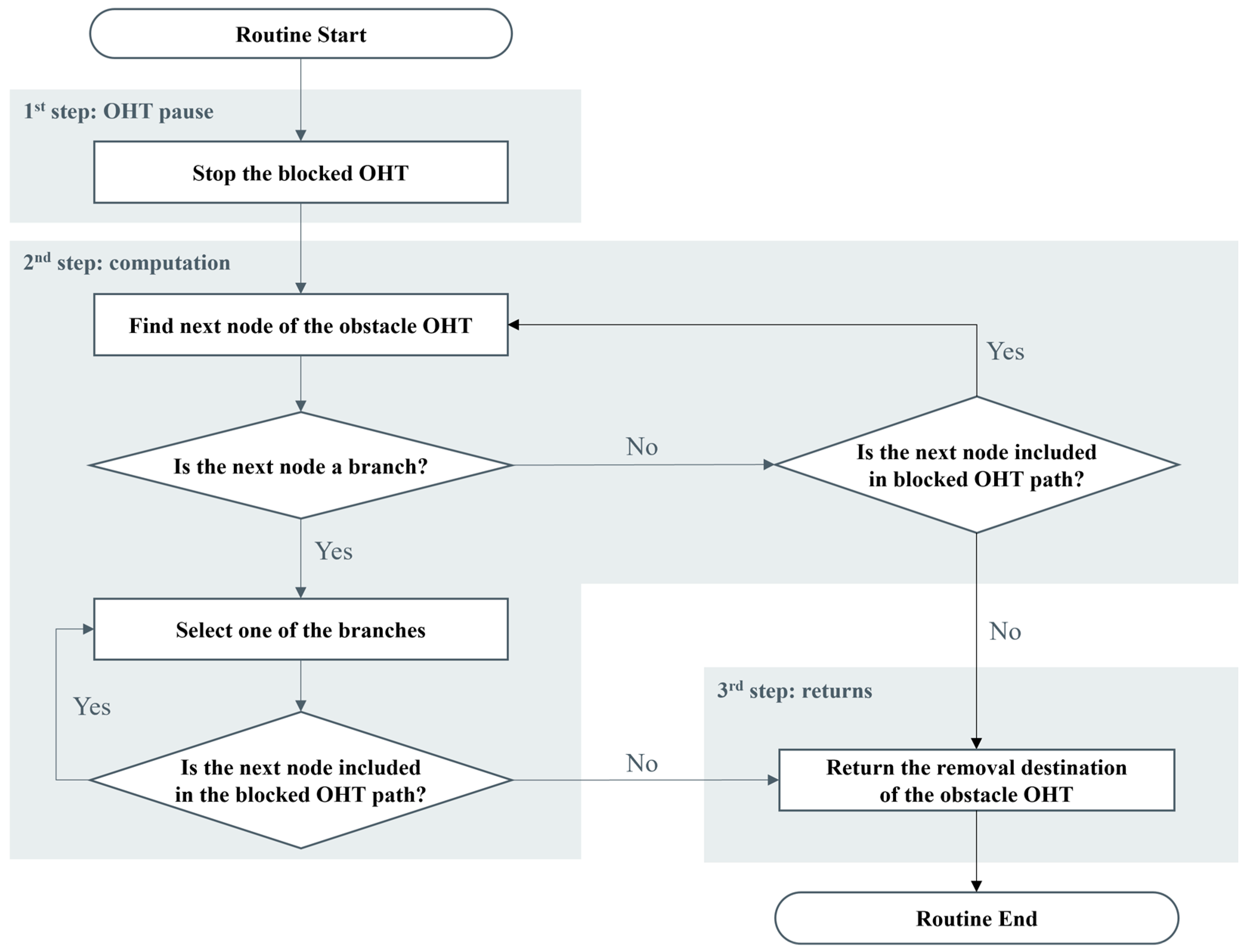
Using the designs following the DEVS formalism, we implemented the models, algorithms, and routines in the DEVSim++ library for simulation. As shown in Figure 9, the models had hierarchical, open, and precise designs and could be easily reconfigured. After modeling, the models were implemented using a DEVSim++ library composed of external transition, internal transition, output, and time advance functions. Algorithms and routines such as job scheduling or go command position calculations were implemented as a functional shape inside the DEVSim++ library. For example, Figure 10 shows a simple routine for the removal of a blocking OHT unit based on the go command. If a moving OHT unit is blocked by idle OHT units, the main controller stops the moving OHT unit and requests go schedules. Next, with the go command sent to a scheduler, the removal of blocking OHT units is computed and planned. The next node of a blocking OHT unit is found and compared with the scheduled path of the moving OHT unit. If the next node is duplicated, the next connected node of the blocking OHT is selected, and the comparison is repeated. For branch nodes, one of the nodes is randomly selected and compared. If this is not repeated, the second step is complete. However, if a duplicate node is detected, another branch node is selected for comparison. With the computed result, the scheduled path is returned to the main controller to move the operating OHT unit away from the blocking one.
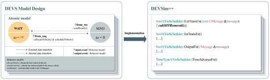
Figure 9.
Proposed model implementation using DEVSim++ library.
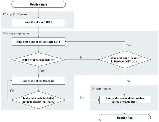
Figure 10.
Routine for removing a blocking OHT unit.
4. Experimental Design for Exploratory Analysis
4.1. Simulation Scenario
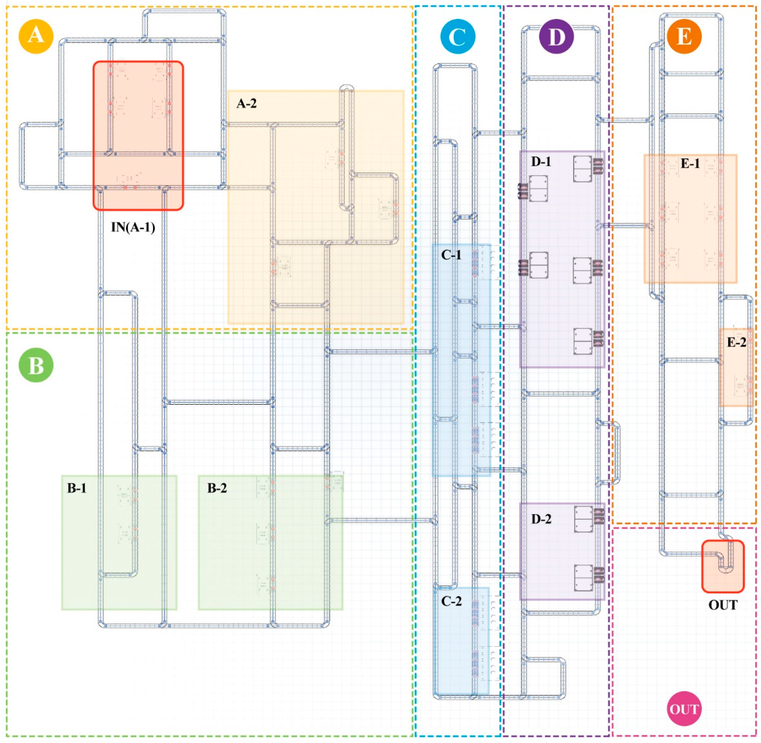
To the best of our knowledge, no consolidated guidelines exist for optimizing the fab configuration. Consequently, guidelines may differ depending on the definition of optimization. Through an exploratory analysis, we aimed to optimize the number of physical systems, such as the number of OHT units and pieces of equipment, in the fab design shown in Figure 11. The process was divided into six regions, from A to E and finally OUT. The simulation started with process A-1 and was finalized with the OUT process. Excluding the OUT process, every other process was divided into regular and repair processes, which were indexed as 1 and 2, respectively (e.g., A-1 is a regular process, and A-2 is a repair process). A repair process could be added depending on the FOUP quality. For example, starting from process A-1, if the FOUP quality was unacceptable, a repair process was added between processes A-1 and D-1. After repair process A-2, the FOUP was moved to process D-1 to resume production. These processes were repeated until the end of the simulation. Table 2 lists the minimum and maximum production sequences. The minimum sequence represents the case where only the regular processes are followed, without any repair processes, while the maximum sequence represents the case where all repair processes are included.
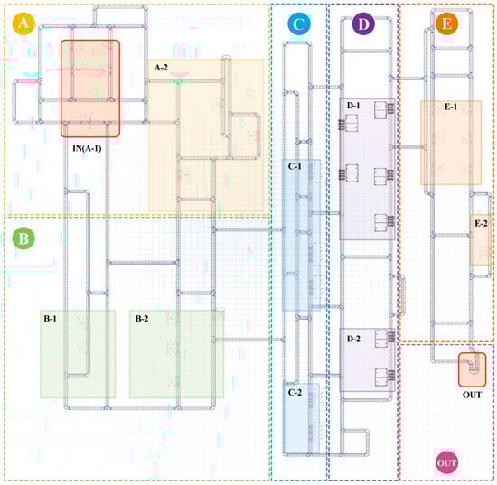
Figure 11.
Experimental fab layout for simulation.
Table 2.
Possible minimum and maximum production sequences.
As mentioned in Section 3, we adopted an exploratory analysis for the simulation results and categorized the three scenarios. First, scenario 1 was used to determine the optimal number of OHT units. Table 3 lists the uncontrollable parameters, which were fixed and applied to all the step-by-step scenarios. Here, the “No. of Levels” column lists the values for the parameter, and the rest of the parameters, except no. of FOUPs, have not been given separate values because the nature of the parameter does not allow for subdivision by type. We chose the DEVS-based simulation model for OHT operation optimization as it allows for easily changing the parameters and it reflects the parameters input into the actual OHT process well, making it quite scalable. For this reason, the parameters speed of OHT, load/unload time, and process time of each equipment in Table 3 are all set to random values, with the possibility of being the most basic. For example, we set the target amount of FOUPs to 300 and the yield acceptance score, which indicates the FOUP quality, to at least 95%.
Table 3.
Uncontrollable simulation parameters.
The controllable simulation parameters are listed in Table 4. Depending on the purpose of the scenario, each parameter was either fixed or controlled. For example, the equipment yield rate was defined as three levels of 95%, 90%, and 85%, which are high, medium, and low, to reflect different FOUP qualities, and a probability function was applied. This parameter reflected the FOUP quality, and a probability function was applied for randomness. The number of OHT units was controlled from two to 20 to find the optimal quantity. In the subsequent scenarios, a stepwise approach was adopted. In scenario 2, the OHT unit count derived from scenario 1 was fixed as a constant parameter, and the number of machines in a specific area was reduced from 12 to two. Then, in scenario 3, the optimal machine count identified in scenario 2 was retained, while the number of machines in another area was decreased from seven to one. By incrementally adjusting these variables, this method effectively manages the complex interactions among parameters and enables a clearer interpretation of the experimental results. The details of this setup are listed in Table 5. Hence, 111 cases were considered over 20 Monte Carlo simulations, and the corresponding KPIs were analyzed. For the data analysis, we set three baselines. First, the lead time should be maintained or improved in comparison with the previous scenario. Second, to ensure system stability, the bottleneck occurrence rate was set to be less than 10% of all transport commands. A comparison between lead time and bottleneck occurrence revealed that when the bottleneck rate exceeded 10%, the lead time tended to exceed the 95% confidence interval, indicating a significant deviation from stable operation. Thirdly, to ensure efficient operation of the OHT units, their utilization rate was set to be at least 90%. An analysis based on queuing theory demonstrated that as OHT unit utilization increased, the system wait time exhibited a nonlinear growth pattern. The rate of increase at 90% utilization was comparable with that at 80%, while being significantly lower than that at 100%, making it an optimal threshold for balancing efficiency and stability. For the simulation, we used a computer equipped with a Windows operating system, an Intel®® Core™ i7-1070H processor at 2.60 GHz, and 16.0 GB of memory. Visual Studio 2019 was used as the integrated development environment.
Table 4.
Controllable simulation parameters.
Table 5.
Equipment information: process time in the simulation and number of required pieces of equipment.
4.2. KPIs
Five KPIs were calculated to compare and assess the simulation results of every scenario. Table 6 lists the calculated KPIs and their descriptions. By analyzing the lead and buffer wait times, we estimated the efficiency of the overall process. For example, a short lead time indicated competitive results for the fab, and a short buffer wait time indicated efficient job scheduling. If many OHT units are used, the lead and buffer wait times can be improved naturally, but using an excessive number of OHT units in a limited space can lead to unnecessary bottlenecks and high costs, thus reducing efficiency. Therefore, the go command rate and OHT unit utilization rate were analyzed together as target KPIs. Below, we describe the KPIs used for a simulation analysis, while the corresponding results are reported and analyzed in Section 5.
Table 6.
Evaluated KPIs.
4.2.1. Lead Time
The lead time is an important KPI for evaluating the manufacturing efficiency. This time includes the buffer wait time of the FOUP, the travel time, and the load/unload time of the OHT units. The lead time per FOUP was calculated using Equation (41), where and represent the controllable parameters of the experiments, with being the number of used OHT units and being the equipment yield rate. In addition, is the FOUP index, is the production start time, and is the production completion time.
4.2.2. Buffer Wait Time
The buffer wait time is the time FOUP spends waiting at the input/output port of the equipment buffer. With an optimized flow of OHT units, this time can be reduced. The buffer wait time per FOUP is given in Equation (42), where is the FOUP index, is the index of visited pieces of equipment, is the process completion time for the piece of equipment, and is the FOUP unload time to the OHT unit. For example, if FOUP 1 visited two pieces of equipment, at 4:00 and 10:00, and the OHT arrived at 6:00 and 12:00, then the total buffer wait time was 4:00.
4.2.3. OHT Unit Utilization Rate
The utilization rate is calculated as the OHT unit’s active time over the simulation time and plays a crucial role in adjusting the optimal number of OHT units for a given fab. If a few OHT units are used and the OHT demand exceeds the capacity, the utilization rate of each OHT unit remains high and the buffer wait time increases. In contrast, if the number of OHT units exceeds the demand, some units remain in an IDLE state and may block the rail, thus causing bottlenecks. The analysis results were calculated using Equation (43), where is the OHT unit index; is the index of the completed command; is the completion time of the command; and is the start time of the command, which includes the traveling and load/unload times.
4.2.4. Equipment Active Time
The equipment active time represents the total uptime of an individual piece of equipment considered in the simulation. We used it to determine whether equipment in a specific process zone was used for an even amount of time. The process time of the individual pieces of equipment was summed as described in Equation (44), where is the index of a piece of equipment, is the processed FOUP index, and is the equipment processing time.
4.2.5. Go Command Rate
The go command rate was analyzed along with the OHT utilization rate. If the number of OHT units was excessive, bottlenecks frequently occurred. Therefore, go commands were delivered to the blocking OHT units. Equation (45) was used to calculate the go command rate, where F is the number of from commands, T is the number of to commands, and G is the number of go commands.
We used Equations (41)–(45) to calculate separate results for the FOUP and physical system. To describe the operation throughout the simulation, the individual values were averaged using Equation (46), where is any of the KPIs given in Equations (41)–(45), is the number of averaged values, and is the number of simulation repetitions. For example, the lead times for a single simulation with 300 values were averaged as shown in Equation (47). For the analysis, we adopted a Monte Carlo simulation and applied Equation (48) in 20 iterations per case to judge the experimental results based on the minimum, average, and maximum values in the iterations according to the central limit theorem. The minimum, average, and maximum values were derived from the set of KPIs determined using Equations (49)–(51).
5. Exploratory Analysis Results
5.1. Simulation Results for Scenario 1
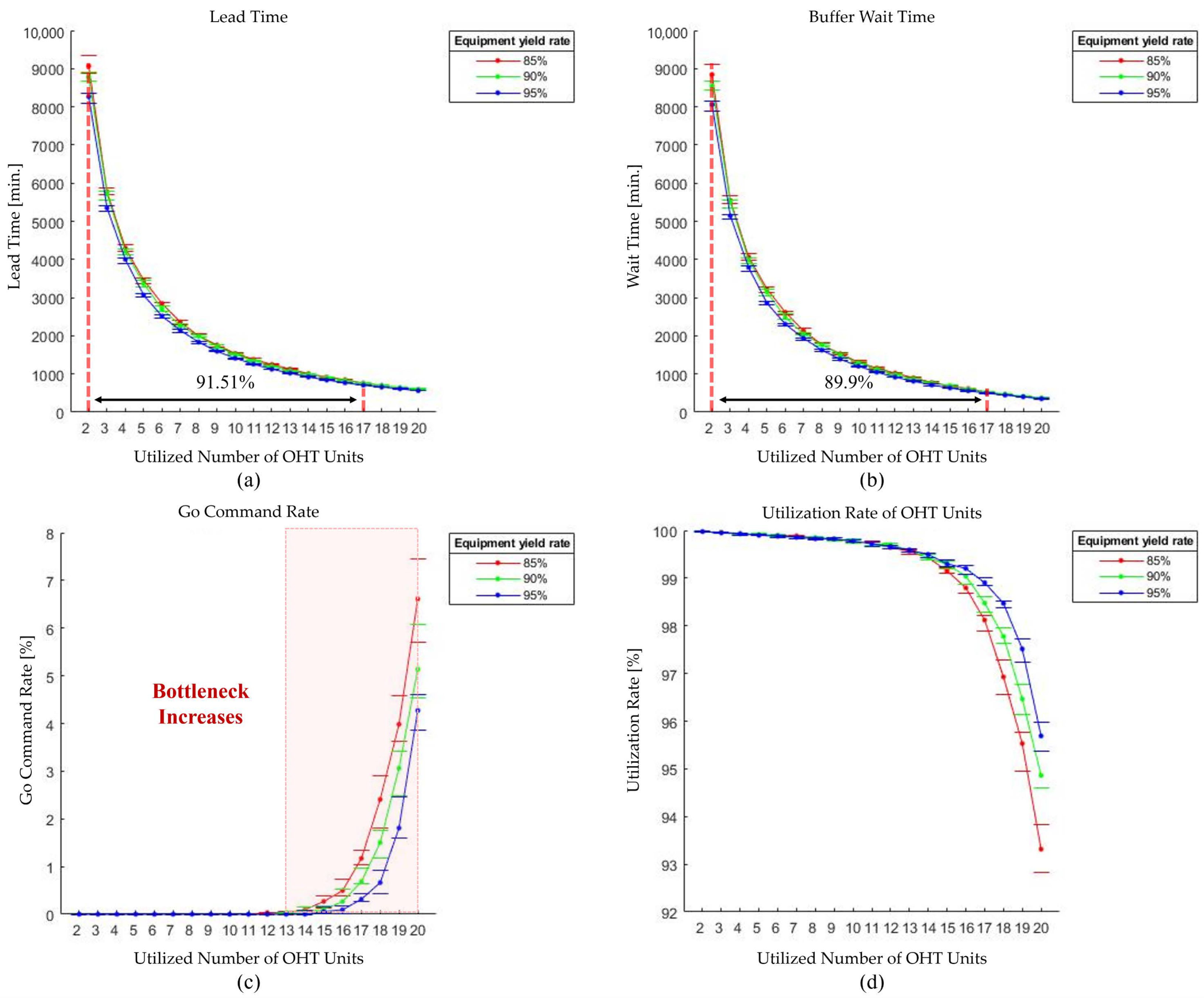
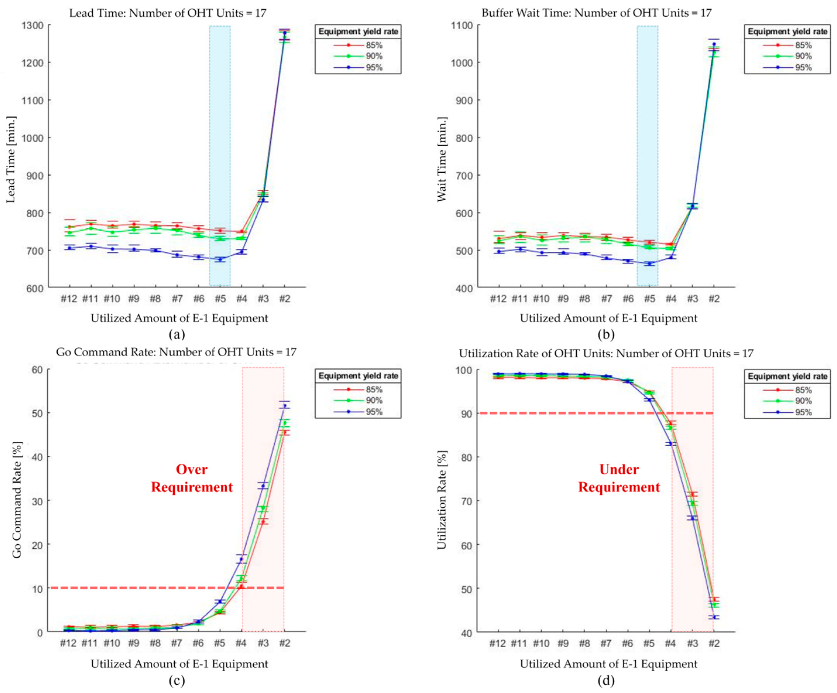
Figure 12 shows the results for scenario 1, which was used to determine the optimal number of OHT units. As shown in Figure 12a,b, the lead and buffer wait times exhibited the same trend. With only a few OHT units, the equipment yield rate affected the experimental results. Because a low equipment yield rate required more repair processes, longer lead and buffer wait times were needed due to the complex path generation. On the other hand, as OHT units were added, the gaps between the equipment yield rates narrowed. Overall, as the number of OHTs increased, the lead and buffer wait times for production tended to improve. The best results were obtained for two or three OHT units, with the lead time being improved by 35.61%. From the 17 utilized OHT units, we observed a negligible improvement in the results (below 0.08%).
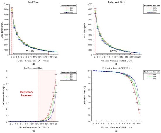
Figure 12.
Experimental results for scenario 1. (a) Lead time, (b) buffer wait time, (c) go command rate, and (d) OHT utilization rate.
As shown in Figure 12c,d, the go command rate was close to 0% and the OHT utilization rate was evenly distributed at a stable low slope for up to 13 OHT units. However, bottlenecks then began to occur, and the OHT utilization rate decreased. Compared with the lead and buffer wait times, more OHT units affected the equipment yield rate, whose minimum-to-maximum gaps became wider. For 17 OHT units, the lead and buffer wait times were 91.51% and 89.9% higher than those for two OHT units, respectively. Despite the equipment yield rate, the go command rate averaged 0.76%, and the OHT utilization rate averaged 98.48%. Therefore, 17 OHT units were selected as the optimal quantity. A series of experiments were conducted using 17 OHTs, identified as the optimal quantity, to compare production rates and determine which equipment should be optimized in scenarios 2 and 3. The analysis revealed an imbalance in equipment utilization patterns, particularly in process E-1 and the OUT process. A closer examination of the equipment operation times showed that certain equipment was overutilized, while other equipment remained underutilized. Based on these findings, scenario 2 was designed to optimize the equipment in the E-1 process, while scenario 3 focused on optimizing the equipment in the OUT process, ensuring more balanced and efficient system operation.
5.2. Simulation Results for Scenario 2
From scenario 1, we analyzed the four KPIs and obtained 17 OHT units as the optimal configuration for the considered fab design. Moreover, by analyzing the total active time of the equipment, we identified that process E-1 and the OUT process were used unevenly, leading to unnecessary costs. For scenario 2, we considered 17 OHT units while varying the amount of equipment in process E-1 from 12 to two.
As shown in Figure 13a,b, by using from 12 to five pieces of equipment for process E-1, the overall equipment yield rate was either largely maintained or even improved. Comparing five with 12 pieces of equipment, the lead time improved by 1.28%, 2.22%, and 4.31% for equipment yield rates of 85%, 90%, and 95%, respectively, and the buffer wait times were 1.91%, 3.54%, and 6.55%, respectively. However, when we further reduced the amount of equipment, the lead and wait times tended to increase, indicating inefficiency. As shown in Figure 13c,d, the go command rate remained below 1% until eight pieces of equipment were used, and the utilization rate remained above 98%. However, for two pieces of equipment, the graphs exhibited drastic changes. In this case, on average, 48.25% of go commands were delivered, and the utilization rate decreased to an average of 45.7% due to bottlenecks. Because the removal of the E-1 equipment is common, a high equipment yield rate had a large effect.
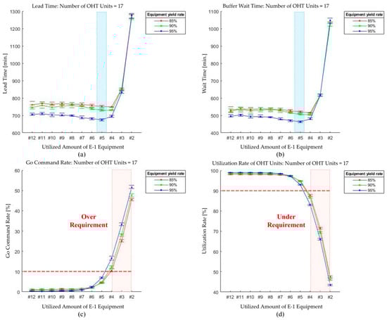
Figure 13.
Experimental results for scenario 2. (a) Lead time, (b) buffer wait time, (c) go command rate, and (d) OHT utilization rate.
To optimize the amount of equipment, we focused on three rules. The most important rule was that (1) the lead time must be maintained at 1% or improved compared with that from the previous scenario. This rule was directly related to the capabilities of the fab. If equipment reduction is excessive, bottlenecks may increase exponentially. Therefore, we set the (2) go command rate to less than 10% for all commands and (3) the OHT unit utilization rate to at least 90% to maintain optimal material flow. By applying these three rules, we determined that five pieces of equipment is the optimal quantity for process E-1. It was determined that reducing the number of equipment leads to a more balanced distribution of workload. However, excessive reductions beyond a certain threshold may increase the OHT wait times and disrupt the equilibrium of equipment utilization in subsequent processes. Specifically, adjusting the number of equipment in process E-1 to five was found to enable optimal operation in terms of KPIs, thereby minimizing adverse effects on downstream processes.
5.3. Simulation Results for Scenario 3
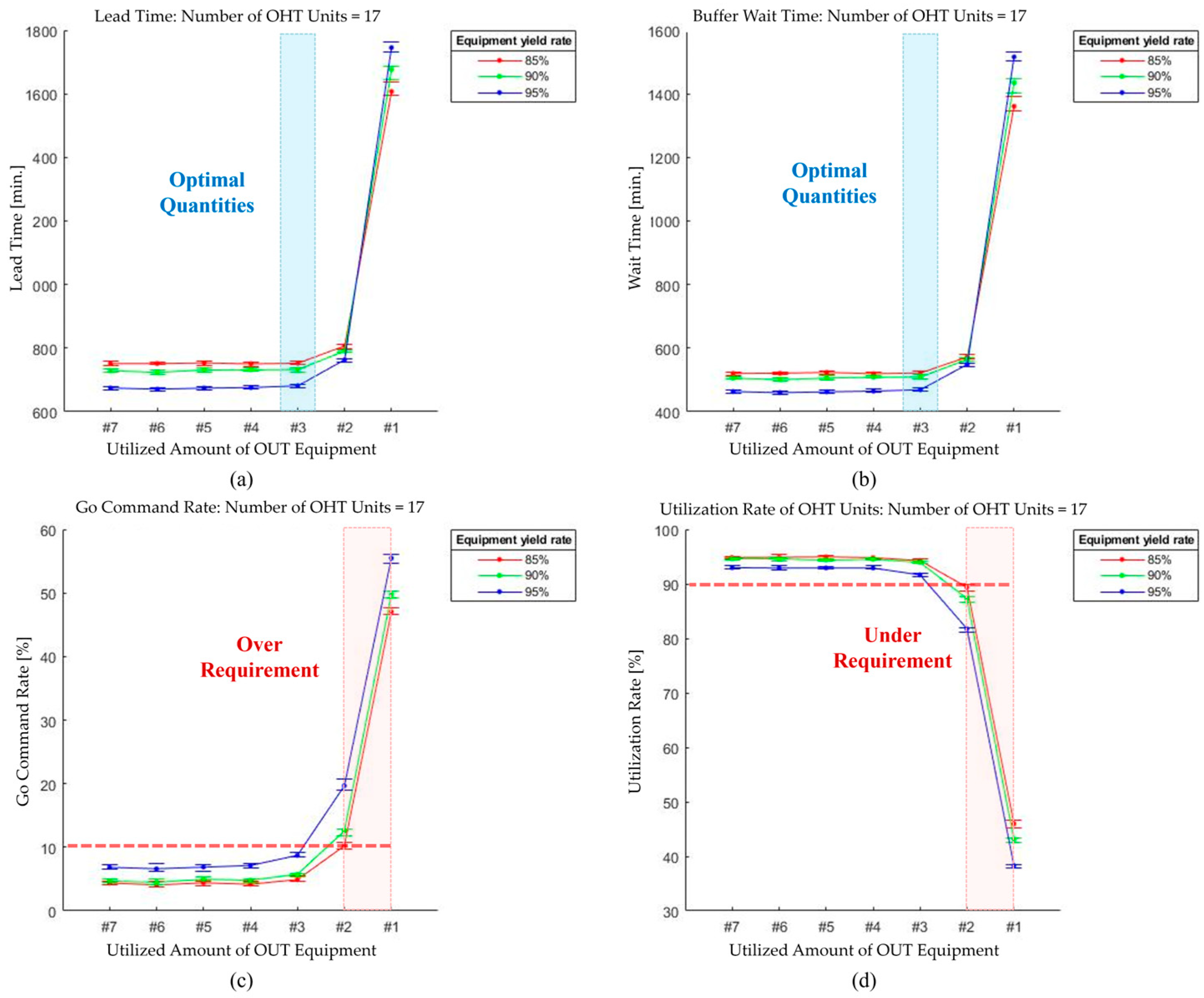
Based on an exploratory analysis conducted through a step-by-step scenario evaluation, we determined that the optimal quantities for the E-1 process were 17 OHT units and five machines, aiming to improve the KPIs. As a next step, in scenario 3, we conducted further experiments by fixing the optimal parameters derived from the exploratory analysis while adjusting the number of machines at the OUT process from seven to one.
As shown in Figure 14a,b, from seven to three pieces of equipment for the OUT process, no notable improvements were observed, but the times slightly decreased under 0.8%, fulfilling the defined rule. In addition, as shown in Figure 14c,d, the rules for the go command and OHT utilization rates were satisfied. For one piece of equipment, the overall KPIs deteriorated with a high slope. Thus, we selected three pieces of equipment as the optimal quantity for the OUT process. However, reducing the amount of equipment by one unit led to a rapid decline in overall KPI performance, suggesting that an excessive reduction in equipment may cause bottlenecks in the production process. Further analysis confirmed that as the amount of equipment decreased, OHT wait times increased and equipment utilization across specific processes became imbalanced. Nevertheless, when the amount of equipment for the OUT process was adjusted to three, OHT wait times were minimized and equipment utilization was more evenly distributed, indicating that this configuration was the most efficient in terms of overall operational performance. Therefore, setting the optimal amount of equipment for the OUT process to three is deemed a reasonable and balanced approach.
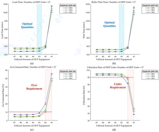
Figure 14.
Experimental results for scenario 3. (a) Lead time, (b) buffer wait time, (c) go command rate, and (d) OHT utilization rate.
6. Discussion
By conducting a step-by-step scenario-based exploratory analysis, we optimized the numbers of OHT units and pieces of equipment for specific process zones. Table 7 lists the optimal results, with the best values highlighted in bold, and Table 8 shows the comparison results, with the average values highlighted in bold. The lead time comparisons between scenario 1 and both scenarios 2 and 3 indicated average improvements of 2.83% and 2.25%, while improvements of 4.31% and 3.6% were observed for the buffer wait time, respectively. However, the reduction in lead times and equipment utilization did not necessarily improve in the same direction. For example, as machine optimization progressed in scenario 1, lead times improved by an average of 2.83%, while OHT utilization decreased by an average of 4.4%. Conversely, in scenario 3, a further reduction in the number of machines resulted in an average 0.6% increase in lead times, accompanied by a tendency to reduce OHT utilization. This suggests that excessive reductions in the number of machines can increase the likelihood of bottlenecks by concentrating work in certain processes, which in turn can increase lead times. In addition, as the number of machines decreased, bottlenecks naturally increased, which also affected the go command rate and OHT utilization. A comparison of scenarios 2 and 3 shows that the go command rate increased by an average of 1.18%, meaning that route optimization of OHTs in certain processes became more important. The results of this study indicate that reducing the number of machines is not necessarily the most effective solution. Rather, the optimal approach is a balanced consideration of lead times, capacity utilization, and OHT utilization. It is worth noting that a significant reduction in the number of machines may result in a concentration of work on a particular process, increasing the likelihood of bottlenecks and consequently increasing lead times. Conversely, effective adjustment of under-utilized equipment within a process minimizes unnecessary movement of OHT units, thereby increasing the likelihood of optimizing the overall logistics flow. Therefore, analyzing equipment utilization by process and considering OHT route optimization in conjunction with process-specific equipment utilization, as opposed to simply reducing the number of machines, to formulate an optimal operational strategy is imperative. From an economic perspective, the implementation of optimization strategies has been demonstrated to exert a profound influence on the operational processes of a manufacturing entity (Table 7). An examination of the go command and the utilization of OHTs reveals that the machine yields in scenarios 1 and 2 intersect. The yield of the machine in these scenarios was found to be 85% and 95%, respectively. This phenomenon can be attributed to the fact that diminished machine yields are prone to necessitating more recurrent repairs, which in turn results in OHTs employing diverse routes and consequently mitigating bottlenecks on specific routes.
Table 7.
KPIs for scenarios 1–3. Bold values: The best values.
Table 8.
KPI comparisons between step-by-step scenarios. Bold values: The average values.
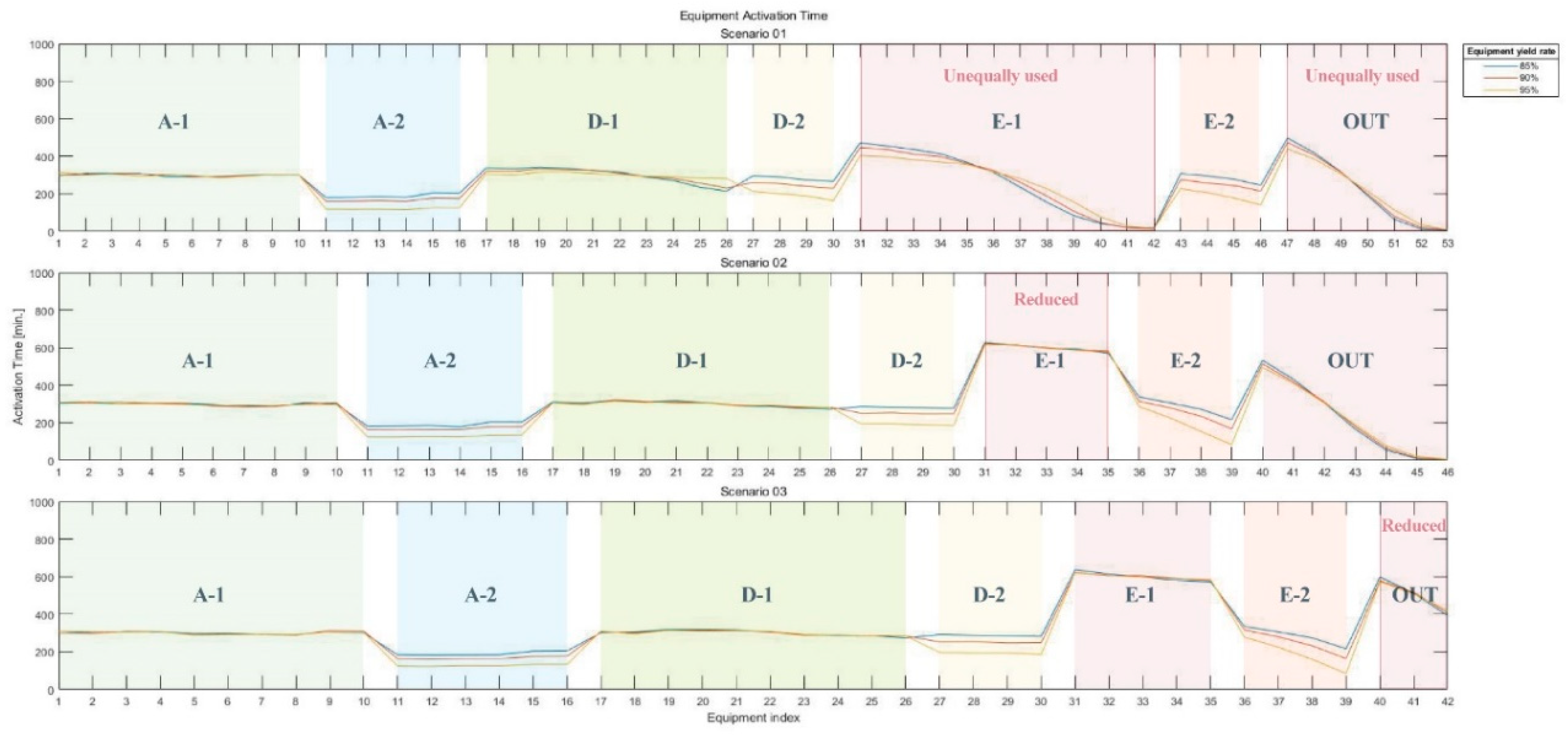
The optimal results may vary depending on the decision made to reduce the amount of equipment in the OUT process via fabs from seven, which is the result of scenario 2, to three, which is the result of scenario 3. By choosing scenario 2 as the optimal case, the lead time can be guaranteed, compared with scenario 3. On the other hand, by selecting scenario 3, the fab can reduce the total amount of equipment, which gives the fab short-term economic benefits. As summarized in Figure 15, as the scenarios evolve from 1 to 3, the evenness of the operation increases. However, by simply removing pieces of equipment, the evenness of operation distributions between process E-2 and the OUT process reaches a limit.

Figure 15.
Total active time of the equipment for scenarios 1–3.
In a real manufacturing environment, it is essential to minimize bottlenecks through OHT route optimization and prevent productivity losses through real-time OHT placement and dynamic route adjustments when equipment productivity is low. The importance of such optimization strategies was also confirmed in a study by Beixin Xia et al. [40]. Beixin Xia et al. [40] proposed an algorithm that optimizes OHT allocation in AMHSs in real time. This algorithm improves the productivity of the fab by dynamically coordinating OHTs and equipment. The research results show that OHT allocation and route optimization can alleviate bottlenecks and improve overall logistics flow. Considering the actual OHT system operation cases, in complex production environments such as large-scale semiconductor fabs, a strategy that comprehensively considers factors such as OHT route optimization, process equipment placement, operational balance, and real-time adjustments is required, rather than considering only individual optimization factors. This study confirmed through scenario analysis that the balance between OHT route optimization and equipment operation affects each other, and that both factors must be considered together to effectively resolve process bottlenecks and maximize productivity.
7. Conclusions
We proposed a simulation model based on the DEVS formalism to create various scenarios and easily perform adjustments. Optimal system operation was achieved using the simulation model. To implement a semiconductor logistics system in the simulation framework, the system was divided into a physical system, a system controller, and an experimental frame. This design allows for easy modification and reconstruction of individual components, facilitating efficient experimentation and scenario expansion. An exploratory analysis was conducted across scenarios 1–3 to determine the optimal number of components in the system. Monte Carlo simulations were performed to statistically analyze various cases. After analyzing the simulation results for five different processes and approximately 50 pieces of equipment, we found that employing 17 OHT units was the optimal quantity for operation. This configuration resulted in an average utilization rate of 98.47% for OHT units. Furthermore, the amount of equipment for process E-1 and the OUT process could be reduced from 12 to five and seven to three, respectively. Therefore, the proposed simulation structure allowed us to optimize the number of OHT units and pieces of equipment to improve operational efficiency. By applying the optimal OHT unit and equipment layout, we can expect to minimize the logistics bottleneck in the semiconductor manufacturing process, shorten lead times, and reduce unnecessary equipment maintenance costs and energy consumption to optimize operating costs. Optimizing semiconductor manufacturing systems requires more than just equipment adjustments. Various factors such as improved scheduling algorithms, equipment and rail relocation, and load balancing must be comprehensively considered. The proposed modular model was designed with this scalability in mind and provides flexibility for easy modification and reconfiguration. For example, the SA manager can be modified to integrate different scheduling algorithms and adjust board configurations and master controllers to optimize system performance. This facilitates application to actual semiconductor manufacturing environments and provides optimization opportunities to maximize productivity and operational efficiency. In addition, this study used a DEVS-based framework to perform flexible and high-fidelity system analyses, bridging the gap between theoretical modeling and the complexity of real semiconductor logistics systems. The DEVS-based framework was used to analyze the semiconductor manufacturing process with high fidelity, and an event-based simulation was used to realistically evaluate the OHT operation and process flow. However, for more realistic modeling, a multi-paradigm approach such as agent-based modeling and system dynamics modeling is expected to provide a more comprehensive interpretation. Future research should consider a wider range of dynamic and stochastic factors and expand upon the decision model to create a more accurate version. Nevertheless, this study used some simplified parameters and has some limitations, such as not being able to experimentally verify the differences with the actual OHT process. Therefore, future research should use more realistic input data and more accurately account for process variability and site conditions to further improve the reliability of the simulation results. Finally, as manufacturing environments become more complex and urgent orders or unexpected equipment failures occur, ensuring optimal operation through simple equipment adjustments alone will become difficult. Therefore, the proposed model should be extended to apply reinforcement learning-based OHT path optimization techniques. For example, techniques such as Deep Q-Network (DQN) or Proximal Policy Optimization (PPO) can be used to automate real-time rerouting of OHTs to optimize OHT placement. However, processes such as accurately modeling the actual semiconductor manufacturing environment and training reinforcement learning require huge amounts of computational resources, and the training time can be excessively long. In addition, reinforcement learning models may not be learned stably in complex manufacturing environments. Therefore, future research should consider a hybrid approach that combines reinforcement learning techniques with conventional rule-based scheduling or use transfer learning techniques that apply pre-trained models from a simulation environment to a real-time operating environment. Such research is expected to further extend the applicability of the proposed framework in real semiconductor manufacturing environments and derive optimal OHT operation and scheduling strategies.
Author Contributions
Conceptualization, J.-H.S.; methodology, J.-H.S. and H.-J.J.; software, J.-H.S., S.-W.C. and B.-G.K.; validation, K.-M.S.; formal analysis, S.-H.J.; investigation, H.-J.J.; resources, B.-G.K.; data curation, S.-H.J.; writing—original draft preparation, S.-H.J.; writing—review and editing, K.-M.S. and B.-G.K.; visualization, S.-W.C.; supervision, K.-M.S.; project administration, B.-G.K. All authors have read and agreed to the published version of the manuscript.
Funding
This work was partly supported by the Technology development Program of MSS [RS-2024-00511378] and conducted with the support of the Korea Institute of Industrial Technology (KITECH) as “RIAM Learning Factory Platform”.
Data Availability Statement
The original contributions presented in this study are included in the article.
Conflicts of Interest
The authors declare no conflicts of interest.
References
- Park, K.T.; Park, Y.H.; Park, M.W.; Noh, S.D. Architectural framework of digital twin-based cyber-physical production system for resilient rechargeable battery production. J. Comput. Des. Eng. 2023, 10, 809–829. [Google Scholar] [CrossRef]
- Hwang, I.; Jang, Y.J. Q (λ) learning-based dynamic route guidance algorithm for overhead hoist transport systems in semiconductor fabs. Int. J. Prod. Res. 2020, 58, 1199–1221. [Google Scholar] [CrossRef]
- Nazzal, D.; El-Nashar, A. Survey of research in modeling conveyor-based automated material handling systems in wafer fabs. In Proceedings of the 2007 Winter Simulation Conference, Washington, DC, USA, 9–12 December 2007. [Google Scholar] [CrossRef]
- Nazzal, D.; McGinnis, L.F. Analytical approach to estimating AMHS performance in 300 mm fabs. Int. J. Prod. Res. 2007, 45, 571–590. [Google Scholar] [CrossRef]
- Wang, C.N. The improvement of lot delivery time in 450 mm semiconductor manufacturing. Appl. Math. Inf. Sci. 2014, 8, 2983. [Google Scholar] [CrossRef]
- Boden, P.; Rank, S.; Schmidt, T. Control of heterogenous AMHS in semiconductor industry under consideration of dynamic transport carrier transfers. In Proceedings of the 22nd IEEE International Conference on Industrial Technology (ICIT), Valencia, Spain, 10–12 March 2021; pp. 1403–1408. [Google Scholar] [CrossRef]
- Tu, Y.M. Short-term scheduling model of cluster tool in wafer fabrication. Mathematics 2021, 9, 1029. [Google Scholar] [CrossRef]
- Huang, C.J.; Chang, K.H.; Lin, J.T. Optimal vehicle allocation for an automated materials handling system using simulation optimization. Int. J. Prod. Res. 2012, 50, 5734–5746. [Google Scholar] [CrossRef]
- Wan, J.; Shin, H. Predictive vehicle dispatching method for overhead hoist transport systems in semiconductor fabs. Int. J. Prod. Res. 2022, 60, 3063–3077. [Google Scholar] [CrossRef]
- Wang, C.N. The preemptive stocker dispatching rule of automatic material handling system in 300 mm semiconductor manufacturing factories. J. Phys. Conf. Ser. 2016, 710, 12033. [Google Scholar] [CrossRef]
- Wu, L. A performance model of automated material handling systems with double closed-loops and shortcuts in 300 mm semiconductor wafer fabrication systems. J. Manuf. Syst. 2021, 58, 316–334. [Google Scholar] [CrossRef]
- Lin, J.T.; Wang, F.K.; Wu, C.K. Simulation analysis of the connecting transport AMHS in a wafer fab. IEEE Trans. Semicond. Manuf. 2003, 16, 555–564. [Google Scholar] [CrossRef]
- Lin, J.T.; Wang, F.K.; Yang, C.J. The performance of the number of vehicles in a dynamic connecting transport AMHS. Int. J. Prod. Res. 2005, 43, 2263–2276. [Google Scholar] [CrossRef]
- Liang, S.K.; Wang, C.N. Modularized simulation for lot delivery time forecast in automatic material handling systems of 300 mm semiconductor manufacturing. Int. J. Adv. Manuf. Technol. 2005, 26, 645–652. [Google Scholar] [CrossRef]
- Mohammadi, M. A queue-based aggregation approach for performance evaluation of a production system with an AMHS. Comput. Oper. Res. 2020, 115, 104838. [Google Scholar] [CrossRef]
- Luan, F.; Cai, Z.; Wu, S.; Liu, S.Q.; He, Y. Optimizing the low-carbon flexible job shop scheduling problem with discrete whale optimization algorithm. Mathematics 2019, 7, 688. [Google Scholar] [CrossRef]
- Motlagh, M.M.; Azimi, P.; Amiri, M.; Madraki, G. An efficient simulation optimization methodology to solve a multi-objective problem in unreliable unbalanced production lines. Expert Syst. Appl. 2019, 138, 112836. [Google Scholar] [CrossRef]
- Teerasoponpong, S.; Sopadang, A. A simulation-optimization approach for adaptive manufacturing capacity planning in small and medium-sized enterprises. Expert Syst. Appl. 2021, 168, 114451. [Google Scholar] [CrossRef]
- Zeigler, B.P.; Praehofer, H.; Kim, T.G. Theory of Modeling and Simulation; Academic Press: Cambridge, MA, USA, 2000. [Google Scholar] [CrossRef]
- Kang, B.G.; Seo, K.M.; Kim, T.G. Model-Based Design of Defense Cyber-Physical Systems to Analyze Mission Effectiveness and Network Performance. IEEE Acces 2019, 7, 42063. [Google Scholar] [CrossRef]
- Seo, K.M.; Hong, W.; Kim, T.G. Enhancing model composability and reusability for entity-level combat simulation: A conceptual modeling approach. Simul. Trans. Soc. Model. Simul. Int. 2017, 93, 825–840. [Google Scholar] [CrossRef]
- Kim, T.G.; Sung, C.H.; Hong, S.Y.; Hong, J.H.; Choi, C.B.; Kim, J.H.; Bae, J.W. DEVSim++ toolset for defense modeling and simulation and interoperation. J. Def. Model. Simul. 2011, 8, 129–142. [Google Scholar] [CrossRef]
- Gupta, S.; Hasenbein, J.J.; Park, S. Improving scheduling and control of the OHTC controller in wafer fab AMHS systems. Simul. Model. Pract. Theory 2021, 107, 102190. [Google Scholar] [CrossRef]
- Wang, C.N.; Hsu, H.P.; Tran, V.V. An improved dispatching method (a-HPDB) for automated material handling system with active rolling belt for 450 mm wafer fabrication. Appl. Sci. 2017, 7, 780. [Google Scholar] [CrossRef]
- Ben-Salem, A.; Yugma, C.; Troncet, E.; Pinaton, J. A simulation-based approach for an effective AMHS design in a legacy semiconductor manufacturing facility. In Proceedings of the 2017 Winter Simulation Conference (WSC), Las Vegas, NV, USA, 3–6 December 2017; pp. 3600–3611. [Google Scholar] [CrossRef]
- Pan, C.; Zhang, J.; Qin, W. Real-time OHT dispatching mechanism for the interbay automated material handling system with shortcuts and bypasses. Chin. J. Mech. Eng. 2017, 30, 663–675. [Google Scholar] [CrossRef]
- Wu, L.; Zhang, Z.; Zhang, J. A hybrid vehicle dispatching approach for unified automated material handling system in 300 mm semiconductor wafer fabrication system. IEEE Access 2019, 7, 174028–174041. [Google Scholar] [CrossRef]
- Qin, W.; Zhang, J.; Sun, Y. Dynamic dispatching for interbay material handling by using modified Hungarian algorithm and fuzzy-logic-based control. Int. J. Adv. Manuf. Technol. 2013, 67, 295–309. [Google Scholar] [CrossRef]
- Huang, C.W.; Lin, J.T. A pre-dispatching vehicle method for a diffusion area in a 300 mm wafer fab. J. Ind. Prod. Eng. 2016, 33, 579–591. [Google Scholar] [CrossRef]
- Qin, W. Dynamic dispatching for interbay automated material handling with lot targeting using improved parallel multiple-objective genetic algorithm. Comput. Oper. Res. 2021, 131, 105264. [Google Scholar] [CrossRef]
- Lee, S.; Kim, Y.; Kahng, H.; Lee, S.K.; Chung, S.; Cheong, T.; Kim, S.B. Intelligent traffic control for autonomous vehicle systems based on machine learning. Expert Syst. Appl. 2020, 144, 113074. [Google Scholar] [CrossRef]
- Lee, Y.H.; Lee, S. Deep reinforcement learning based scheduling within production plan in semiconductor fabrication. Expert Syst. Appl. 2022, 191, 116222. [Google Scholar] [CrossRef]
- Chen, H.; Luo, F.; Zhou, J.; Dong, Y. Multi-Objective Optimized GPSR Intelligent Routing Protocol for UAV Clusters. Mathematics 2024, 12, 2672. [Google Scholar] [CrossRef]
- Chen, Y.; Shao, C.H.; Wu, S.C.; Chang, C. Decentralized dispatching for blocking avoidance in automated material handling systems. In Proceedings of the Winter Simulation Conference (WSC), Washington, DC, USA, 11–14 December 2016. [Google Scholar] [CrossRef]
- Ben-Salem, A.; Yugma, C.; Troncet, E.; Pinaton, J. AMHS Design for reticles in photolithography area of an existing wafer fab: IE: Industrial engineering. In Proceedings of the 2016 27th Annual SEMI Advanced Semiconductor Manufacturing Conference (ASMC), Saratoga Springs, NY, USA, 16–19 May 2016; pp. 110–115. [Google Scholar] [CrossRef]
- Lee, K.W.; Chang, D.S.; Park, S.C. Material handling system modeling of a modern FAB. In Proceedings of the 10th International Conference on Computer Modeling and Simulation, Sydney, Australia, 8–10 January 2018; pp. 271–275. [Google Scholar] [CrossRef]
- Choi, S.H.; Seo, K.M.; Kim, T.G. Accelerated Simulation of Discrete Event Dynamic Systems via a Multi-Fidelity Modeling Framework. Appl. Sci. 2017, 7, 1056. [Google Scholar] [CrossRef]
- Lee, J.Y.; Lee, K.; Park, S. Virtual commissioning for an Overhead Hoist Transporter in a semiconductor FAB. Int. J. Prod. Res. 2020, 58, 6890–6898. [Google Scholar] [CrossRef]
- Bernd, W.; Thomas, A.; Thomas, B.K.A. Production scheduling in complex job shops from an Industrie 4.0 perspective: A review and challenges in the semiconductor industry. In Proceedings of the SamI40 Workshop at i-KNOW, International Conference on Knowledge Technologies and Data-Driven Business—I-KNOW 2016 (i-KNOW 2016), Graz, Austria, 18–19 October 2016; Available online: https://zenodo.org/records/495155 (accessed on 28 January 2025).
- Xia, B.; Tian, T.; Gao, Y.; Zhang, M.; Peng, Y. A Dynamic Dispatching Method for Large-Scale Interbay Material Handling Systems of Semiconductor FAB. Sustainability 2022, 14, 13882. [Google Scholar] [CrossRef]

Disclaimer/Publisher’s Note: The statements, opinions and data contained in all publications are solely those of the individual author(s) and contributor(s) and not of MDPI and/or the editor(s). MDPI and/or the editor(s) disclaim responsibility for any injury to people or property resulting from any ideas, methods, instructions or products referred to in the content. |
© 2025 by the authors. Licensee MDPI, Basel, Switzerland. This article is an open access article distributed under the terms and conditions of the Creative Commons Attribution (CC BY) license (https://creativecommons.org/licenses/by/4.0/).