Some Exact Results on Lindley Process with Laplace Jumps

Abstract

We consider a Lindley process with Laplace-distributed space increments. We obtain closed-form recursive expressions for the density function of the position of the process and for its first exit time distribution from the domain $[0,h]$. We illustrate the results in terms of the parameters of the process. An example of the application of the analytical results is discussed in the framework of the CUSUM method.

1. Introduction

Random walk has attracted mathematicians’ attention both for its analytical properties and for its role in modeling instances ever since it was mentioned by Pearson [1]. Presently, random walks are universally recognized as the simplest example of a stochastic process and are used as a simplified version of more complex models. For modeling purposes, it is often necessary to introduce suitable boundary conditions, constraining the evolution of the process in specific regions. Typical conditions are absorbing or reflecting boundaries and the involved random walk may be in one or more dimensions. The recurrence of the states of the free or bounded process in one or more dimensions has been the subject of past and recent studies, and results are available for the free random walk [2] or in the presence of specific boundaries [3].

The distribution of a simple random walk at Time $n,n=1,2,\cdots$ has a simple expression while, in the case of the distribution of the random walk constrained by two absorbing boundaries, it involves important calculation efforts [4].

Classical methods for the study of random walks refer to their Markov property. This happens, for example, when the focus is on recurrence properties in one or more dimensions. Alternatively, some results can be obtained by means of diffusion limits that give good approximations under specific hypotheses [5,6,7,8] or allow the determination of asymptotic results for problems such as the maximum of a random walk or the first exit time across general boundaries [9]. However, the presence of boundaries often determines combinatorics problems and discourages the search for closed-form solutions. Furthermore, the switch from unitary jumps to continuous jumps introduces important computational difficulties. There are thousands of papers about random walk, and it is impossible to refer to all of them. We limit ourselves to citing the recent excellent review by Dshalalow and White [10] that lists many of the most important available results.

In this paper, we focus on a particular constrained random walk: the Lindley process [11]. In particular, we prove a set of analytical results about it. This process is a discrete-time random walk characterized by continuous jumps with a specified distribution.

Without loss of generality, we define it as

$$\begin{array}{ccc}\hfill W_n& =& max(0,W_{n-1}+Z_{n-1})n\ge 1\hfill \\ \hfill W_0& =& x\ge 0.\hfill \end{array}$$

(1)

where $\{Z_n,n\ge 0\}$ are i.i.d. random variables.

Modeling interest for the Lindley process arises in several fields. Historically, it was introduced in [11] to describe waiting times experienced by customers in a queue over time and it has been extensively studied in recent decades [12,13,14].

This process also arises in a reliability context, in a sequential test framework, through the study of CUSUM tests [15]. Moreover, the same process appears in problems related to resources management [16] and in highlighting atypical regions in biological sequences, transferring biological sequence analysis tools to break-point detection for on-line monitoring [17].

Many contributions concerning properties of the Lindley process are motivated by their important role in applications [2,11,16,18,19]. A large part of the papers about the Lindley process concerns its asymptotic behavior. Using the strong law of large numbers, in 1952, Lindley [11] in the framework of queuing theory showed that the process admits a limit distribution as n diverges if and only if $\mathbb{E}\left[Z\right]<0$, i.e., if the customer’s arrival rate is slower than the service one. Furthermore, when $\mathbb{E}\left[Z\right]=0$, the ratio $W_n/\sqrt{n}$ converges to the modulus of a Gaussian random variable. Lindley also showed that the limit distribution is the solution of an integral equation, and Kendall solved it in the case of exponential arrivals [14] while Erlang determined its expression when both arrival and service times are exponential [20]. Simulations were used in [21] to determine invariant distribution when $Z_i,i=1,2,\cdots$ are Laplace or Gaussian distributed. The analytical expression of the limit distribution was determined by Stadje [22] for the case of integer-valued increments. Recent contributions consider recurrence properties in higher dimensions [3,23,24] or the study of the rate of convergence of expected values of functions of the process.

Other contributions make use of stochastic ordering notion [25] or of continuous-time versions of the Lindley process [12]. Recently, the use of machine learning techniques has been proposed to learn Lindley recursion (1) directly from the waiting time data of a G/G/1 queue [26]. Furthermore, Lakatos and Zbaganu [25], and Raducan, Lakatos and Zbaganu [27] introduced a class of computable Lindley processes for which the distribution of the space increments is a mixture of two distributions. To the best of our knowledge, no other analytical expressions are available for a Lindley process.

Concerning the first exit time problem for the Lindley process, it has been considered mainly in the framework of CUSUM methodology to detect the time in which a change in the parameters of the process happens [15,28,29,30]. In this context, the focus was on the Average Run Length that corresponds to the exit time of the process from a boundary, and in [31,32], such distribution and its expected value are determined when the $Z_i,i=1,2,\cdots$ are exponentially distributed with a shift. Markovich and Razumchick [33] investigated a problem related to first exit times, i.e., the appearance of clusters of extremes defined as subsequent experiences of high thresholds in a Lindley process.

Here, we consider a Lindley process characterized by Laplace-distributed space increments $Z\sim Laplace(\mu ,\sigma )$, i.e., Z distributed as a Laplace random variable characterized by parameter $\mu$ and scale parameter $\sigma$,

$$f_Z\left(z\right)={\displaystyle \frac{e^{-\frac{|z-\mu |}{\sigma }}}{2\sigma }},$$

(2)

where the mean and the variance are $\mathbb{E}\left(Z\right)=\mu$ and $V\left(Z\right)=2{\sigma }^2$.

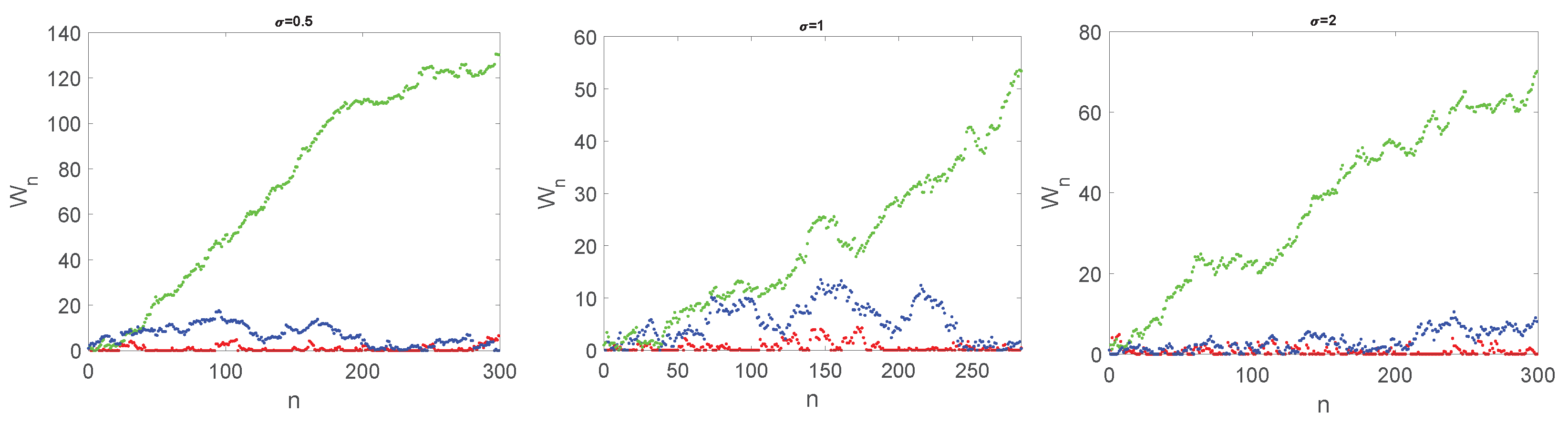
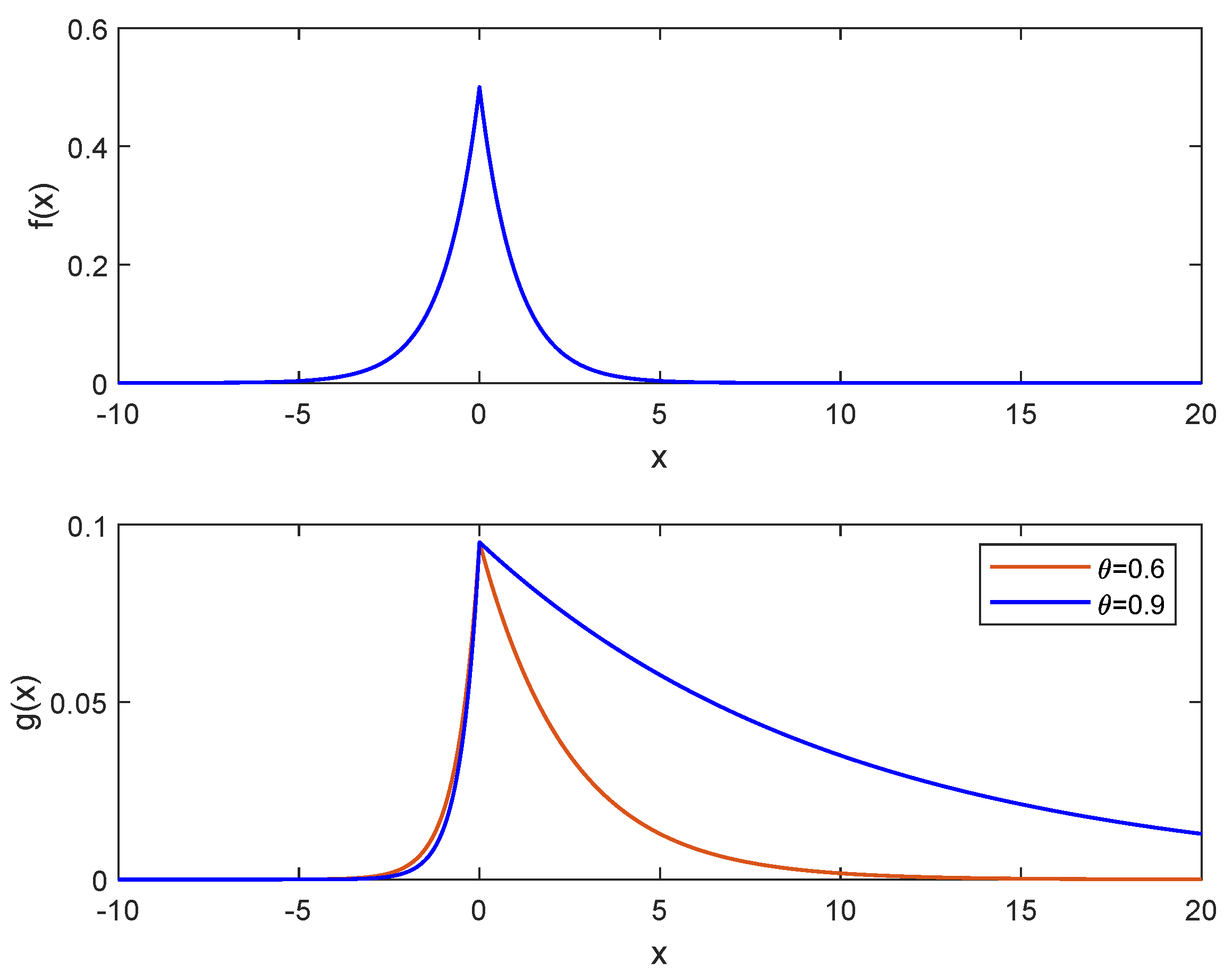
In Figure 1, three trajectories are plotted of the Lindley process with $\sigma =1$, $x=1$, and different values of $\mu$. The Laplace distribution is often used to model the distribution of financial assets and market fluctuations. It is also used in signal processing and communication theory to model noise and other random processes. Additionally, the Laplace distribution has been used in image processing and speech recognition.

As in the case of the simple random walk, here, the behavior of the random walk dramatically changes according to the sign of $\mu$. Indeed, it is well known [9] that, when $\mu >0$, all the states are transient, and the process has a drift toward infinity. However, in the case $\mu =0$, the process is null recurrent, and when $\mu <0$, the process is positive recurrent and admits limit distribution. Such distribution is the solution of the Lindley integral equation [11]. Unfortunately, the analytical solution is unknown and numerical methods become necessary.

The recurrence properties imply certainty of the first exit time of the process W from $[0,h]$ for each $h>x$, and the study of the first exit time distribution can be performed.

Here, our aim is to derive expressions for the distribution of the process as the time evolves together with its first exit time (FET) from $[0,h]$. Taking advantage of the presence of exponential in the Laplace distribution, we prove recursive closed-form formulae for such distributions, and we show that different formulae hold on different parameters domain. We underline that the special expression of the Laplace distribution allows the use of recursion in various steps of our proofs. This makes hard the extension to other types of distributions. In Section 2 and Section 3, we study the distribution of the process and its first exit times from $[0,h]$, respectively. In these sections, we do not present any proofs that we postpone in Section 4 and Section 5. Due to the complexity of the derived exact formulae for the studied distributions, we complete our work implementing the software necessary for fast computation of the formulae of interest. This software is open source and can be found in the GitHub repository [34]. In Section 6, we illustrate the role of the parameters of the Laplace distribution on the position and FET distribution of the Lindley process. Lastly, in Section 7, we present an application of our theoretical results in the CUSUM framework. In particular, we discuss a method to detect the change point when the data moves from a symmetric Laplace distribution to an asymmetric one.

2. Distribution of $W_n$

Let us consider the Lindley process (1) with Laplace-distributed jumps (2). In the following, we will use the distribution of the process at Time $n\ge 0$ that we denote as

$$F_n\left(u\right|x):=F_{W_n}\left(u\right|x)=\mathbb{P}(W_n\le u|W_0=x).$$

and, with an abuse of notation, we indicate with

$$f_n\left(u\right|x):=f_{W_n}\left(u\right|x)={\displaystyle \frac{\partial }{\partial u}}\mathbb{P}(W_n\le u|W_0=x).$$

the corresponding probability density function, since the derivative is the distributional derivative because the $W_n$ are mixed random variables.

In the following we make use of Dirac delta function $\delta \left(u\right)$ with the agreement that, for each $x>0$

$${\int }_0^{x}f\left(u\right)\delta \left(u\right)=f\left(0\right).$$

Since $W_n\ge 0$, the density $f_n\left(u\right|x)=0$ for $u<0$. Moreover, if $a>b$ the sum ${\sum }_{i=a}^b{f}_i=0$.

Lemma 1.

The probability distribution function of $W_1$ for $\mu >-x$ is

$$\begin{array}{c}\hfill F_1\left(u\right|x)=F_{W_1}\left(u\right|x)=\left\{\begin{array}{cc}0\hfill & u<0\hfill \\ {\displaystyle \frac{1}{2}}{e}^{-{\displaystyle \frac{\mu -u+x}{\sigma }}}\hfill & 0\le u\le x+\mu \hfill \\ 1-{\displaystyle \frac{1}{2}}{e}^{{\displaystyle \frac{\mu -u+x}{\sigma }}}\hfill & u>x+\mu \hfill \end{array}\right.\end{array}$$

(3)

while, for $\mu \le -x$ is

$$\begin{array}{c}\hfill F_1\left(u\right|x)=F_{W_1}\left(u\right|x)=\left\{\begin{array}{cc}0\hfill & u<0\hfill \\ 1-{\displaystyle \frac{1}{2}}{e}^{{\displaystyle \frac{\mu -u+x}{\sigma }}}\hfill & u\ge 0\hfill \end{array}\right.\end{array}$$

(4)

The corresponding probability density function is

$$\begin{array}{c}\hfill f_1\left(u\right|x)=f_{W_1}\left(u\right|x)=\left\{\begin{array}{cc}{\displaystyle \frac{e^{-\frac{|u-x-\mu |}{\sigma }}}{2\sigma }}{\mathbb{1}}_{(0,+\infty )}\left(u\right)+{\displaystyle \frac{e^{-\frac{(x+\mu )}{\sigma }}}{2}}\delta \left(u\right)\hfill & x>-\mu \hfill \\ {\displaystyle \frac{e^{-\frac{u-x-\mu }{\sigma }}}{2\sigma }}{\mathbb{1}}_{(0,+\infty )}\left(u\right)+\left(1-{\displaystyle \frac{e^{\frac{(x+\mu )}{\sigma }}}{2}}\right)\delta \left(u\right)\hfill & x\le -\mu \hfill \end{array}\right.\end{array}$$

(5)

where $\delta \left(u\right)$ is the Dirac delta function.

Remark 1.

Using the Markov property of the process W, the one-step transition probability density function, for $n\ge 0$, is

$$\begin{array}{cc}\hfill f(u,n+1|y,n)& :={\displaystyle \frac{\partial }{\partial u}}\mathbb{P}(W_{n+1}\le u|W_n=y)=f_1\left(u\right|y)\hfill \\ \hfill & =\left\{\begin{array}{cc}{\displaystyle \frac{e^{-\frac{|u-y-\mu |}{\sigma }}}{2\sigma }}{\mathbb{1}}_{(0,+\infty )}\left(u\right)+{\displaystyle \frac{e^{-\frac{(y+\mu )}{\sigma }}}{2}}\delta \left(u\right)\hfill & y>-\mu \hfill \\ {\displaystyle \frac{e^{-\frac{u-y-\mu }{\sigma }}}{2\sigma }}{\mathbb{1}}_{(0,+\infty )}\left(u\right)+\left(1-{\displaystyle \frac{e^{\frac{(y+\mu )}{\sigma }}}{2}}\right)\delta \left(u\right)\hfill & y\le -\mu \hfill \end{array}\right.\hfill \end{array}$$

(6)

Notation 1.

In the forthcoming, when not necessary, we will skip the dependence on the initial position of the process: $F_n\left(u\right|x)=F_n\left(u\right)$, $f_n\left(u\right|x)=f_n\left(u\right)$.

To determine the distribution of $W_n$, computations change according to the sign of $\mu$. Theorem 1 gives the distribution for $\mu >0$. When $\mu$ is negative two different cases arise when $-x<\mu$ (Theorem 2) and $\mu >-x$ (Theorem 3).

Theorem 1.

For a Lindley process $\{W_n,n\ge 0\}$ characterized by Laplace increments with location parameter $\mu \ge 0$, the probability density function of the position is given by

$$\begin{array}{}\hfill \mathrm{(7a)}& \hfill f_n\left(u\right)& =\sum _{i=0}^{n+1}{f}_n^i\left(u\right),u\ge 0,n\ge 1\hfill \hfill \mathrm{(7b)}& \hfill f_0\left(u\right)& =\delta (u-x)\hfill \end{array}$$

where

$$\begin{array}{}\hfill \mathrm{(8a)}& \hfill & f_n^i\left(u\right)=\left\{\sum _{j=0}^{m_n^i-1}{\displaystyle \frac{1}{{\left(2\sigma \right)}^n}}\left[a_n^{(i,j)}{(u-n\mu )}^j{e}^{{\displaystyle \frac{u}{\sigma }}}+b_n^{(i,j)}{(u-n\mu )}^j{e}^{-{\displaystyle \frac{u}{\sigma }}}\right]\right\}{\mathbb{1}}_{I_n^i}\left(u\right)1\le i\le n+1\hfill \hfill \mathrm{(8b)}& \hfill & f_n^0\left(u\right)=c_n\delta \left(u\right)\hfill \end{array}$$

$m_n^i=min(n,i)$ and $I_n^i$, $i=1,\cdots n+1$, with ${\bigcup }_{i=1}^{n+1}{I}_n^i=(0,+\infty )$, are

$$\begin{array}{}\hfill \mathrm{(9a)}& \hfill & I_n^i=((i-1)\mu ,i\mu ]i=1,\cdots ,n-1\hfill \hfill \mathrm{(9b)}& \hfill & I_n^n=((n-1)\mu ,n\mu +x]\hfill \hfill \mathrm{(9c)}& \hfill & I_n^{n+1}=(n\mu +x,+\infty ),\hfill \end{array}$$

The coefficients $a_{n+1}^{(i,j)}$, $b_{n+1}^{(i,j)}$ and $c_{n+1}$ verify the following recursive relations for $1\le i\le n+1$, $1\le j\le m_n^i-1$

$$\begin{array}{cc}\hfill \mathrm{(10a)}& \hfill a_{n+1}^{(i,j)}& =e^{-{\displaystyle \frac{\mu }{\sigma }}}\left[\sum _{k=j-1}^{m_n^{i-1}-1}{(-1)}^{k+j}{a}_n^{\left(\right(i-1),k)}{\displaystyle \frac{k!}{j!}}{\left({\displaystyle \frac{2}{\sigma }}\right)}^{k-j+1}\right]\hfill \hfill \mathrm{(10b)}& \hfill b_{n+1}^{(i,j)}& =-e^{{\displaystyle \frac{\mu }{\sigma }}}\left[\sum _{k=j-1}^{m_n^{i-1}-1}{b}_n^{\left(\right(i-1),k)}{\displaystyle \frac{k!}{j!}}{\left({\displaystyle \frac{2}{\sigma }}\right)}^{k-j+1}\right]\hfill \hfill a_{n+1}^{(i,0)}& =e^{-{\displaystyle \frac{\mu }{\sigma }}}\left[\sum _{j=i}^{n+1}{A}_j^{\left(2\right)}+\sum _{k=0}^{m_n^{i-1}-1}\left[a_n^{\left(\right(i-1),k)}\left({\displaystyle \frac{{\left((i-1-n)\mu \right)}^{k+1}}{k+1}}+{(-1)}^{k}k!{\left({\displaystyle \frac{\sigma }{2}}\right)}^{k+1}\right)\right.\right.\hfill \\ \hfill \mathrm{(10c)}& \hfill & \left.-b_n^{\left(\right(i-1),k)}{\displaystyle \frac{e^{\frac{-2n\mu }{\sigma }}{\sigma }^{k+1}}{2^{k+1}}}\left[\Gamma \left(1+k,{\displaystyle \frac{2\left(\right(i-1-n\left)\mu \right)}{\sigma }}\right)\right]+c_n{\delta }_{i,1}\right]\hfill \hfill b_{n+1}^{(i,0)}& =e^{{\displaystyle \frac{\mu }{\sigma }}}\left[\sum _{j=1}^{i-2}{A}_j^{\left(1\right)}-\sum _{k=0}^{m_n^{i-1}-1}\left[b_n^{\left(\right(i-1),k)}\left({\displaystyle \frac{{\left((i-2-n)\mu \right)}^{k+1}}{k+1}}-k!{\left({\displaystyle \frac{\sigma }{2}}\right)}^{k+1}\right)\right]\right.\hfill \\ \hfill \mathrm{(10d)}& \hfill & \left.-a_n^{\left(\right(i-1),k)}{\displaystyle \frac{e^{\frac{2n\mu }{\sigma }}{\sigma }^{k+1}{(-1)}^k}{2^{k+1}}}\left[\Gamma \left(1+k,{\displaystyle \frac{-2\left(\right(i-1-n\left)\mu \right)}{\sigma }}\right)\right]+c_n(1-{\delta }_{i,1})\right]\hfill \hfill c_{n+1}& ={\displaystyle \frac{e^{-\frac{\mu }{\sigma }}}{2{\left(2\sigma \right)}^n}}\left\{\sum _{j=1}^{n+1}\sum _{k=0}^{m_n^i-1}\left[{\left.a_n^{(j,k)}{\displaystyle \frac{{(y-n\mu )}^{k+1}}{k+1}}\right|}_{I_n^j}-b_n^{(j,k)}{\displaystyle \frac{e^{-\frac{2n\mu }{\sigma }}{\sigma }^{k+1}}{2^{k+1}}}{\left.\Gamma \left(1+k,{\displaystyle \frac{2(y-n\mu )}{\sigma }}\right)\right|}_{I_n^j}\right]\right.\hfill \\ \hfill \mathrm{(10e)}& \hfill & +\left.{\left(2\sigma \right)}^n{c}_n\right\}\hfill \end{array}$$

where ${\delta }_{i,j}$ is the Kronecker delta and

$$\begin{array}{}\hfill \mathrm{(11a)}& \hfill A_j^{\left(1\right)}& :={\left.A_j^{\left(1\right)}\left(y\right)\right|}_{I_n^j}=\sum _{k=0}^{m_n^j-1}\left\{a_n^{(j,k)}{\displaystyle \frac{e^{\frac{2n\mu }{\sigma }}{\sigma }^{k+1}{(-1)}^k}{2^{k+1}}}\left[{\left.\Gamma \left(1+k,{\displaystyle \frac{-2(y-n\mu )}{\sigma }}\right)\right|}_{I_n^j}\right]+b_n^{(j,k)}{\left.{\displaystyle \frac{{(y-n\mu )}^{k+1}}{k+1}}\right|}_{I_n^j}\right\}\hfill \hfill \mathrm{(11b)}& \hfill A_j^{\left(2\right)}& :={\left.A_j^{\left(2\right)}\left(y\right)\right|}_{I_n^j}=\sum _{k=0}^{m_n^j-1}\left\{a_n^{(j,k)}{\left.{\displaystyle \frac{{(y-n\mu )}^{k+1}}{k+1}}\right|}_{I_n^j}-b_n^{(j,k)}{\displaystyle \frac{e^{\frac{-2n\mu }{\sigma }}{\sigma }^{k+1}}{2^{k+1}}}\left[{\left.\Gamma \left(1+k,{\displaystyle \frac{2(y-n\mu )}{\sigma }}\right)\right|}_{I_n^j}\right]\right\}.\hfill \end{array}$$

The initial values for the recursion of (10) are

$$\begin{array}{}\hfill \mathrm{(12a)}& \hfill & c_1={\displaystyle \frac{e^{-\frac{\mu +x}{\sigma }}}{2}}\hfill \hfill \mathrm{(12b)}& \hfill & a_1^{(1,0)}=e^{-{\displaystyle \frac{\mu +x}{\sigma }}}\hfill \hfill \mathrm{(12c)}& \hfill & b_1^{(1,0)}=a_1^{(2,0)}=0\hfill \hfill \mathrm{(12d)}& \hfill & b_1^{(2,0)}=e^{{\displaystyle \frac{\mu +x}{\sigma }}}\hfill \end{array}$$

Remark 2.

Observe that the coefficients $a_n^{(n+1,k)}\equiv 0$, for each admissible k. This prevents the terms in (10e) and (11b) to explode.

The following corollary may be useful for computational purposes.

Corollary 1.

The constant coefficients $c_n$, $n=1,2,\cdots$ can also be obtained as

$$c_{n+1}=\sigma f_{n+1}^1\left(0^{+}\right).$$

(13)

Remark 3.

Observe that the density (7) refers to a mixed random variable.

Theorem 2.

For a Lindley process $\{W_n,n\ge 0\}$ characterized by Laplace increments with location parameter $-x<\mu <0$, the probability density function of the position is given by

$$\begin{array}{}\hfill \mathrm{(14a)}& \hfill f_n\left(u\right)& =\sum _{i=0}^2{f}_n^i\left(u\right),u\ge 0,n\ge 1\hfill \hfill \mathrm{(14b)}& \hfill f_0\left(u\right)& =\delta (u-x)\hfill \end{array}$$

where

$$\begin{array}{}\hfill \mathrm{(15a)}& \hfill & f_n^i\left(u\right)=\left\{\sum _{j=0}^{n-1}{\displaystyle \frac{1}{{\left(2\sigma \right)}^n}}\left[a_n^{(i,j)}{(u-n\mu )}^j{e}^{{\displaystyle \frac{u}{\sigma }}}+b_n^{(i,j)}{(u-n\mu )}^j{e}^{-{\displaystyle \frac{u}{\sigma }}}\right]\right\}{\mathbb{1}}_{I_n^i}\left(u\right)i=1,2\hfill \hfill \mathrm{(15b)}& \hfill & f_n^0\left(u\right)=c_n\delta \left(u\right)\hfill \end{array}$$

and $I_n^i$, $i=1,2$ are

$$\begin{array}{}\hfill \mathrm{(16a)}& \hfill & I_n^1=(0,max(0,n\mu +x))\hfill \hfill \mathrm{(16b)}& \hfill & I_n^2=(max(0,n\mu +x),+\infty )\hfill \end{array}$$

• If $x+n\mu >0$, the coefficients $a_{n+1}^{(i,j)}$, $b_{n+1}^{(i,j)}$ verify the recursive relations for $i=1,2$ and $1\le j\le n$

  $$\begin{array}{cc}\hfill \mathrm{(17a)}& \hfill a_{n+1}^{(i,j)}& =e^{-{\displaystyle \frac{\mu }{\sigma }}}\left[\sum _{k=j-1}^{n-1}{(-1)}^{k+j}{a}_n^{(i,k)}{\displaystyle \frac{k!}{j!}}{\left({\displaystyle \frac{\sigma }{2}}\right)}^{k-j+1}\right]\hfill \hfill \mathrm{(17b)}& \hfill b_{n+1}^{(i,j)}& =e^{{\displaystyle \frac{\mu }{\sigma }}}\left[\sum _{k=j-1}^{n-1}{b}_n^{(i,k)}{\displaystyle \frac{k!}{j!}}{\left({\displaystyle \frac{\sigma }{2}}\right)}^{k-j+1}\right]\hfill \hfill a_{n+1}^{(1,0)}& =e^{-{\displaystyle \frac{\mu }{\sigma }}}\left[B_2+\sum _{k=0}^{n-1}\left[a_n^{(1,k)}\left({\displaystyle \frac{{\left(x\right)}^{k+1}}{k+1}}+{(-1)}^{k}k!{\left({\displaystyle \frac{\sigma }{2}}\right)}^{k+1}\right)\right.\right.\hfill \\ \hfill \mathrm{(17c)}& \hfill & \left.-b_n^{(1,k)}{\displaystyle \frac{e^{\frac{-2n\mu }{\sigma }}{\sigma }^{k+1}}{2^{k+1}}}\left[\Gamma \left(1+k,{\displaystyle \frac{2x}{\sigma }}\right)\right]\right]\hfill \hfill b_{n+1}^{(1,0)}& =e^{{\displaystyle \frac{\mu }{\sigma }}}\left[\sum _{k=0}^{n-1}\left[b_n^{(1,k)}\left(-{\displaystyle \frac{{(-n\mu )}^{k+1}}{k+1}}+k!{\left({\displaystyle \frac{\sigma }{2}}\right)}^{k+1}\right)\right]\right.\hfill \\ \hfill \mathrm{(17d)}& \hfill & \left.-a_n^{(1,k)}{\displaystyle \frac{e^{\frac{2n\mu }{\sigma }}{\sigma }^{k+1}{(-1)}^k}{2^{k+1}}}\left[\Gamma \left(1+k,{\displaystyle \frac{2n\mu }{\sigma }}\right)\right]+{\left(2\sigma \right)}^n{c}_n\right]\hfill \hfill \mathrm{(17e)}& \hfill a_{n+1}^{(2,0)}& =0\hfill \hfill b_{n+1}^{(2,0)}& =e^{{\displaystyle \frac{\mu }{\sigma }}}\left[B_1+\sum _{k=0}^{n-1}\left[b_n^{(2,k)}\left(-{\displaystyle \frac{x^{k+1}}{k+1}}+k!{\left({\displaystyle \frac{\sigma }{2}}\right)}^{k+1}\right)\right]\right.\hfill \\ \hfill \mathrm{(17f)}& \hfill & \left.-a_n^{(2,k)}{\displaystyle \frac{e^{\frac{2n\mu }{\sigma }}{\sigma }^{k+1}{(-1)}^k}{2^{k+1}}}\left[\Gamma \left(1+k,-{\displaystyle \frac{2x}{\sigma }}\right)\right]+{\left(2\sigma \right)}^n{c}_n\right]\hfill \end{array}$$

  where

  $$\begin{array}{}\hfill \mathrm{(18a)}& \hfill B_1& =\sum _{k=0}^{n-1}\left\{a_n^{(1,k)}{\displaystyle \frac{e^{\frac{2n\mu }{\sigma }}{\sigma }^{k+1}{(-1)}^k}{2^{k+1}}}\left[{\left.\Gamma \left(1+k,{\displaystyle \frac{-2(y-n\mu )}{\sigma }}\right)\right|}_0^{x+n\mu }\right]+b_n^{(1,k)}{\left.{\displaystyle \frac{{(y-n\mu )}^{k+1}}{k+1}}\right|}_0^{x+n\mu }\right\}\hfill \hfill \mathrm{(18b)}& \hfill B_2& =\sum _{k=0}^{n-1}\left\{b_n^{(2,k)}{\displaystyle \frac{e^{\frac{-2n\mu }{\sigma }}{\sigma }^{k+1}}{2^{k+1}}}\left[\Gamma \left(1+k,{\displaystyle \frac{2x}{\sigma }}\right)\right]\right\}\hfill \end{array}$$
  The values of coefficients $c_{n+1}$ for $n\ge 1$ are

  $$c_{n+1}={\tilde{c}}_{n+1}+{\tilde{\tilde{c}}}_{n+1}$$

  where

  $$\begin{array}{cc}\hfill & {\tilde{c}}_{n+1}=\left\{{\displaystyle \frac{1}{{\left(2\sigma \right)}^n}}\sum _{k=0}^{n-1}\left[a_n^{(1,k)}{e}^{{\displaystyle \frac{2n\mu }{\sigma }}}{\sigma }^{k+1}{(-1)}^k\left[{\left.\Gamma \left(1+k,{\displaystyle \frac{-(y-n\mu )}{\sigma }}\right)\right|}_0^{x+n\mu }\right]\right.\right.\hfill \\ \hfill & \left.+b_n^{(1,k)}{e}^{-{\displaystyle \frac{2n\mu }{\sigma }}}{\sigma }^{k+1}\left[{\left.\Gamma \left(1+k,{\displaystyle \frac{(y-n\mu )}{\sigma }}\right)\right|}_0^{x+n\mu }\right]\right]\hfill \\ \hfill & -{\displaystyle \frac{e^{\frac{\mu }{\sigma }}}{2^{n+1}{\sigma }^n}}\sum _{k=0}^{n-1}\left[a_n^{(1,k)}{\displaystyle \frac{e^{\frac{2n\mu }{\sigma }}{\sigma }^{k+1}{(-1)}^k}{2^{k+1}}}\left[{\left.\Gamma \left(1+k,{\displaystyle \frac{-2(y-n\mu )}{\sigma }}\right)\right|}_0^{x+n\mu }\right]+b_n^{(1,k)}{\left.{\displaystyle \frac{{(y-n\mu )}^{k+1}}{k+1}}\right|}_0^{x+n\mu }\right]\hfill \\ \hfill & +{\displaystyle \frac{1}{{\left(2\sigma \right)}^n}}\sum _{k=0}^{n-1}\left[a_n^{(2,k)}{e}^{{\displaystyle \frac{2n\mu }{\sigma }}}{\sigma }^{k+1}{(-1)}^k\left[{\left.\Gamma \left(1+k,{\displaystyle \frac{-(y-n\mu )}{\sigma }}\right)\right|}_{x+n\mu }^{-\mu }\right]\right.\hfill \\ \hfill & \left.+b_n^{(2,k)}{e}^{-{\displaystyle \frac{2n\mu }{\sigma }}}{\sigma }^{k+1}\left[{\left.\Gamma \left(1+k,{\displaystyle \frac{(y-n\mu )}{\sigma }}\right)\right|}_{x+n\mu }^{-\mu }\right]\right]\hfill \\ \hfill & -{\displaystyle \frac{e^{\frac{\mu }{\sigma }}}{2^{n+1}{\sigma }^n}}\sum _{k=0}^{n-1}\left[a_n^{(2,k)}{\displaystyle \frac{e^{\frac{2n\mu }{\sigma }}{\sigma }^{k+1}{(-1)}^k}{2^{k+1}}}\left[{\left.\Gamma \left(1+k,{\displaystyle \frac{-2(y-n\mu )}{\sigma }}\right)\right|}_{x+n\mu }^{-\mu }\right]+b_n^{(2,k)}{\left.{\displaystyle \frac{{(y-n\mu )}^{k+1}}{k+1}}\right|}_{x+n\mu }^{-\mu }\right]\hfill \\ \hfill & +{\displaystyle \frac{e^{-\frac{\mu }{\sigma }}}{2^{n+1}{\sigma }^n}}\sum _{k=0}^{n-1}\left[b_n^{(2,k)}{\displaystyle \frac{e^{-\frac{2n\mu }{\sigma }}{\sigma }^{k+1}}{2^{k+1}}}\Gamma \left(1+k,-{\displaystyle \frac{2(n+1)\mu }{\sigma }}\right)\right]+\left.\left[\left(1-{\displaystyle \frac{e^{\frac{\mu }{\sigma }}}{2}}\right)c_n\right]\right\}{\mathbb{1}}_{[0,-(n+1\left)\mu \right)}\left(x\right)\hfill \end{array}$$

  (19)

  and

  $$\begin{array}{cc}\hfill & {\tilde{\tilde{c}}}_{n+1}=\left\{{\displaystyle \frac{1}{{\left(2\sigma \right)}^n}}\sum _{k=0}^{n-1}\left[a_n^{(1,k)}{e}^{{\displaystyle \frac{2n\mu }{\sigma }}}{\sigma }^{k+1}{(-1)}^k\left[{\left.\Gamma \left(1+k,{\displaystyle \frac{-(y-n\mu )}{\sigma }}\right)\right|}_0^{-\mu }\right]\right.\right.\hfill \\ \hfill & \left.+b_n^{(1,k)}{e}^{-{\displaystyle \frac{2n\mu }{\sigma }}}{\sigma }^{k+1}\left[{\left.\Gamma \left(1+k,{\displaystyle \frac{(y-n\mu )}{\sigma }}\right)\right|}_0^{-\mu }\right]\right]\hfill \\ \hfill & -{\displaystyle \frac{e^{\frac{\mu }{\sigma }}}{2^{n+1}{\sigma }^n}}\sum _{k=0}^{n-1}\left[a_n^{(1,k)}{\displaystyle \frac{e^{\frac{2n\mu }{\sigma }}{\sigma }^{k+1}{(-1)}^k}{2^{k+1}}}\left[{\left.\Gamma \left(1+k,{\displaystyle \frac{-2(y-n\mu )}{\sigma }}\right)\right|}_0^{-\mu }\right]+b_n^{(1,k)}{\left.{\displaystyle \frac{{(y-n\mu )}^{k+1}}{k+1}}\right|}_0^{-\mu }\right]\hfill \\ \hfill & +{\displaystyle \frac{e^{-\frac{\mu }{\sigma }}}{2^{n+1}{\sigma }^n}}\sum _{k=0}^{n-1}\left[{\left.a_n^{(1,k)}{\displaystyle \frac{{(y-n\mu )}^{k+1}}{k+1}}\right|}_{-\mu }^{x+n\mu }+b_n^{(1,k)}{\displaystyle \frac{e^{-\frac{2n\mu }{\sigma }}{\sigma }^{k+1}}{2^{k+1}}}\left[{\left.\Gamma \left(1+k,{\displaystyle \frac{2(y-n\mu )}{\sigma }}\right)\right|}_{-\mu }^{x+n\mu }\right]\right]\hfill \\ \hfill & +{\displaystyle \frac{e^{-\frac{\mu }{\sigma }}}{2^{n+1}{\sigma }^n}}\sum _{k=0}^{n-1}\left[b_n^{(2,k)}{\displaystyle \frac{e^{-\frac{2n\mu }{\sigma }}{\sigma }^{k+1}}{2^{k+1}}}\Gamma \left(1+k,{\displaystyle \frac{2x}{\sigma }}\right)\right]+\left.\left[\left(1-{\displaystyle \frac{e^{\frac{\mu }{\sigma }}}{2}}\right)c_n\right]\right\}{\mathbb{1}}_{[-(n+1\left)\mu \right),\infty )}\left(x\right)\hfill \end{array}$$

  (20)
  The initial conditions for the recursion of the coefficients are

  $$\begin{array}{}\hfill \mathrm{(21a)}& \hfill & a_1^{(1,0)}=e^{-{\displaystyle \frac{\mu +x}{\sigma }}}\hfill \hfill \mathrm{(21b)}& \hfill & b_1^{(1,0)}=0\hfill \hfill \mathrm{(21c)}& \hfill & a_1^{(2,0)}=0\hfill \hfill \mathrm{(21d)}& \hfill & b_1^{(2,0)}=e^{{\displaystyle \frac{\mu +x}{\sigma }}}\hfill \hfill \mathrm{(21e)}& \hfill & c_1={\displaystyle \frac{e^{-\frac{\mu +x}{\sigma }}}{2}}\hfill \end{array}$$
• If $x+n\mu <0$, we have $f_n^1\left(u\right)\equiv 0$ for each n and the coefficients $a_{n+1}^{(2,j)}$, $b_{n+1}^{(2,j)}$ verify the following recursive relations for $1\le j\le n$.

  $$\begin{array}{cc}\hfill \mathrm{(22a)}& \hfill a_{n+1}^{(2,j)}& =0\hfill \hfill \mathrm{(22b)}& \hfill b_{n+1}^{(2,j)}& =e^{{\displaystyle \frac{\mu }{\sigma }}}\left[\sum _{k=j-1}^{n-1}{b}_n^{(2,k)}{\displaystyle \frac{k!}{j!}}{\left({\displaystyle \frac{\sigma }{2}}\right)}^{k-j+1}\right]\hfill \hfill \mathrm{(22c)}& \hfill a_{n+1}^{(2,0)}& =0\hfill \hfill \mathrm{(22d)}& \hfill b_{n+1}^{(2,0)}& =e^{{\displaystyle \frac{\mu }{\sigma }}}\left[\sum _{k=0}^{n-1}\left[b_n^{(2,k)}\left(-{\displaystyle \frac{{(-n\mu )}^{k+1}}{k+1}}+k!{\left({\displaystyle \frac{\sigma }{2}}\right)}^{k+1}\right)\right.\left.-a_n^{(2,k)}{\displaystyle \frac{e^{\frac{2n\mu }{\sigma }}{\sigma }^{k+1}{(-1)}^k}{2^{k+1}}}\Gamma \left(1+k,{\displaystyle \frac{2n\mu }{\sigma }}\right)\right]+{\left(2\sigma \right)}^n{c}_n\right]\hfill \hfill c_{n+1}& ={\displaystyle \frac{1}{{\left(2\sigma \right)}^n}}\sum _{k=0}^{n-1}\left[b_n^{(2,k)}{e}^{-{\displaystyle \frac{2n\mu }{\sigma }}}{\sigma }^{k+1}\left[{\left.\Gamma \left(1+k,{\displaystyle \frac{(y-n\mu )}{\sigma }}\right)\right|}_0^{-\mu }\right]\right]-{\displaystyle \frac{e^{\frac{\mu }{\sigma }}}{2^{n+1}{\sigma }^n}}\sum _{k=0}^{n-1}\left[b_n^{(2,k)}{\left.{\displaystyle \frac{{(y-n\mu )}^{k+1}}{k+1}}\right|}_0^{-\mu }\right]\hfill \\ \hfill \mathrm{(22e)}& \hfill & +{\displaystyle \frac{e^{-\frac{\mu }{\sigma }}}{2^{n+1}{\sigma }^n}}\sum _{k=0}^{n-1}\left[b_n^{(2,k)}{\displaystyle \frac{e^{-\frac{2n\mu }{\sigma }}{\sigma }^{k+1}}{2^{k+1}}}\Gamma \left(1+k,{\displaystyle \frac{-2(n+1)\mu }{\sigma }}\right)\right]+\left[\left(1-{\displaystyle \frac{e^{\frac{\mu }{\sigma }}}{2}}\right)c_n\right]\hfill \end{array}$$

  with initial conditions given by (21c), (21d) and (21e).

Theorem 3.

For a Lindley process $\{W_n,n\ge 0\}$ characterized by Laplace increments with location parameter $\mu \le -x$, the probability density function of the position is given by

$$\begin{array}{}\hfill \mathrm{(23a)}& \hfill f_n\left(u\right)& =\sum _{i=0}^1{f}_n^i\left(u\right),u\ge 0,n\ge 1\hfill \hfill \mathrm{(23b)}& \hfill f_0\left(u\right)& =\delta (u-x)\hfill \end{array}$$

where

$$\begin{array}{}\hfill \mathrm{(24a)}& \hfill & f_n^1\left(u\right)=\left\{\sum _{j=0}^{n-1}{\displaystyle \frac{1}{{\left(2\sigma \right)}^n}}{b}_n^{(1,j)}{(u-(n-1)\mu )}^j{e}^{-{\displaystyle \frac{u}{\sigma }}}\right\}{\mathbb{1}}_{I_n^1}\left(u\right)\hfill \hfill \mathrm{(24b)}& \hfill & f_n^0\left(u\right)=c_n\delta \left(u\right)\hfill \end{array}$$

and $I_n^1=(0,+\infty ]$.

The coefficients $c_{n+1}$ and $b_{n+1}^{(i,j)}$ verify the following recursive relations for $j=1,\cdots ,n$

$$\begin{array}{cc}\hfill \mathrm{(25a)}& \hfill b_{n+1}^{(1,j)}& =e^{{\displaystyle \frac{\mu }{\sigma }}}\left[\sum _{k=j-1}^{n-1}{b}_n^{\left(\right(1,k)}{\displaystyle \frac{k!}{j!}}{\left({\displaystyle \frac{\sigma }{2}}\right)}^{k-j+1}\right]\hfill \hfill \mathrm{(25b)}& \hfill b_{n+1}^{(i,0)}& =e^{{\displaystyle \frac{\mu }{\sigma }}}\left[\sum _{k=0}^{n-1}\left[b_n^{(1,k)}\left(-{\displaystyle \frac{{[-(n-1)\mu ]}^{k+1}}{k+1}}+k!{\left({\displaystyle \frac{\sigma }{2}}\right)}^{k+1}\right)\right]+{\left(2\sigma \right)}^n{c}_n\right]\hfill \hfill c_{n+1}& =-{\displaystyle \frac{e^{-\frac{\mu }{\sigma }}}{2^{n+1}{\sigma }^n}}\sum _{k=0}^{n-1}{b}_n^{(1,k)}{\displaystyle \frac{e^{-\frac{2(n-1)\mu }{\sigma }}{\sigma }^{k+1}}{2^{k+1}}}\left[{\left.\Gamma \left(1+k,{\displaystyle \frac{2(y-(n-1\left)\mu \right)}{\sigma }}\right)\right|}_{-\mu }^{\infty }\right]\hfill \\ \hfill & -{\displaystyle \frac{1}{{\left(2\sigma \right)}^n}}\sum _{k=0}^{n-1}{b}_n^{(1,k)}{e}^{-{\displaystyle \frac{(n-1)\mu }{\sigma }}}{\sigma }^{k+1}\left[{\left.\Gamma \left(1+k,{\displaystyle \frac{(y-(n-1\left)\mu \right)}{\sigma }}\right)\right|}_0^{-\mu }\right]\hfill \\ \hfill \mathrm{(25c)}& \hfill & -{\displaystyle \frac{e^{\frac{\mu }{\sigma }}}{2^{n+1}{\sigma }^n}}\sum _{k=0}^{n-1}{b}_n^{(1,k)}\left[{\left.{\displaystyle \frac{{(y-(n-1)\mu )}^{k+1}}{k+1}}\right|}_0^{-\mu }\right]+\left[\left(1-{\displaystyle \frac{e^{\frac{\mu }{\sigma }}}{2}}\right)c_n\right].\hfill \end{array}$$

The initial values for the recursion are

$$\begin{array}{cc}\hfill & l{c}_1=\left(1-{\displaystyle \frac{1}{2}}{e}^{{\displaystyle \frac{\mu +x}{\sigma }}}\right)\hfill \\ \hfill & b_1^{(1,0)}=e^{{\displaystyle \frac{\mu +x}{\sigma }}}.\hfill \end{array}$$

3. First Exit Time of ${\mathit{W}}_{\mathit{n}}$

Let $N_x:={min}_{n>0}\left\{W_n\ge h|W_0=x\right\}$ be the first exit time (FET) of the Lindley process (1) from the domain $[0,h]$ for fixed $h>0$ and let $P\left(n\right|x):=\mathbb{P}[N_x=n]$ indicate the probability that the FET is equal to n, $n>0$, given that the process starts in $x\in [0,h)$.

In order to determine the distribution of N, computations change according to the sign of $\mu$ and its order with respect to h. Theorem 4 gives the distribution for $0<\mu <h$ while Corollary 2 considers the case $0<h\le \mu$. For $\mu <0$, Theorem 5 gives the distribution for $-\mu <h$ while Corollary 3 considers the case $0<h<-\mu$ and Theorem 6 refers to $\mu =0$.

Theorem 4.

For a Lindley process $\{W_n,n\ge 0\}$ characterized by Laplace increments with location parameter $0<\mu <h$, the probability distribution of the FET through h is given by

$$P\left(n\right|x)=\sum _{i=1}^{{\ell }_n}{P}_i\left(n\right|x),n>0,0\le x<h$$

(26)

where ${\ell }_n:=min\{n+1,⌈{\displaystyle \frac{h}{\mu }}⌉\}$ and

$$\begin{array}{cc}\hfill & P_i\left(n\right|x)=\left\{\sum _{j=0}^{m_n^i-1}{\displaystyle \frac{1}{2^n{\sigma }^{n-1}}}\left[{\alpha }_n^{(i,j)}{(x+n\mu )}^j{e}^{{\displaystyle \frac{x}{\sigma }}}+{\beta }_n^{(i,j)}{(x+n\mu )}^j{e}^{-{\displaystyle \frac{x}{\sigma }}}\right]+{\eta }_n^{(i,0)}\right\}{\mathbb{1}}_{I_n^i}\left(x\right)1\le i\le {\ell }_n.\hfill \end{array}$$

(27)

Here $m_n^i:=min(n,{\ell }_n-i+1)$ and we partition the interval $[0,h)$ in

$$\begin{array}{cc}\hfill & I_n^i=[h-({\ell }_n-i+1)\mu ,h-({\ell }_n-i)\mu )i=2,\cdots ,{\ell }_n\hfill \\ \hfill & I_n^1=[0,h-({\ell }_n-1)\mu ).\hfill \end{array}$$

(28)

The coefficients ${\alpha }_{n+1}^{(i,j)}$, ${\beta }_{n+1}^{(i,j)}$ and ${\eta }_{n+1}^{(i,0)}$ are defined by the following recursive relations for $1\le i\le {\ell }_{n+1}$ and $1\le j\le m_{n+1}^i-1$

$$\begin{array}{cc}\mathrm{(29a)}& \hfill & {\alpha }_{n+1}^{(i,0)}=e^{{\displaystyle \frac{\mu }{\sigma }}}\left\{\sum _{j=i^{*}+1}^{{\ell }_n}{K}_n^j\right.+\sum _{k=0}^{m_n^{i^{*}}-1}\left[{\alpha }_n^{(i^{*},k)}\left({\displaystyle \frac{{(h-({\ell }_n-i^{*})\mu +n\mu )}^{k+1}}{k+1}}+k!{\displaystyle \frac{{\sigma }^{k+1}{(-1)}^k}{2^{k+1}}}\right)\right.\hfill \hfill & -\left.{\beta }_n^{(i^{*},k)}{\displaystyle \frac{e^{\frac{2n\mu }{\sigma }}{\sigma }^{k+1}}{2^{k+1}}}\left.\Gamma \left(1+k,{\displaystyle \frac{2(h-({\ell }_n-i^{*})\mu +n\mu )}{\sigma }}\right)\right]-{\eta }_n^{(i^{*},0)}{\left(2\sigma \right)}^n{e}^{-{\displaystyle \frac{h-({\ell }_n-i^{*})\mu }{\sigma }}}\right\}\hfill \\ \mathrm{(29b)}& \hfill & {\alpha }_{n+1}^{(i,j)}=-e^{{\displaystyle \frac{\mu }{\sigma }}}\sum _{k=j-1}^{m_n^{i^{*}}-1}{\alpha }_n^{(i^{*},k)}{\left(-{\displaystyle \frac{\sigma }{2}}\right)}^{k-j+1}{\displaystyle \frac{k!}{j!}}\hfill \mathrm{(29c)}& \hfill & {\beta }_{n+1}^{(i,0)}=e^{-{\displaystyle \frac{\mu }{\sigma }}}\left\{\sum _{j=0}^{i^{*}-1}{K}_n^j\right.+\sum _{k=0}^{m_n^{i^{*}}-1}\left[-{\alpha }_n^{(i^{*},k)}{\displaystyle \frac{e^{\frac{-2n\mu }{\sigma }}{\sigma }^{k+1}{(-1)}^k}{2^{k+1}}}\Gamma \left(1+k,{\displaystyle \frac{-2(h-({\ell }_n-i^{*}+1)\mu +n\mu )}{\sigma }}\right)\right.\hfill \hfill & \left.\left.+{\beta }_n^{(i^{*},k)}\left(-{\displaystyle \frac{{(h-({\ell }_n-i^{*}+1)\mu +n\mu )}^{k+1}}{k+1}}+k!{\displaystyle \frac{{\sigma }^{k+1}}{2^{k+1}}}\right)\right]-{\eta }_n^{(i^{*},0)}{\left(2\sigma \right)}^n{e}^{{\displaystyle \frac{h-({\ell }_n-i^{*}+1)\mu }{\sigma }}}\right\}\hfill \\ \mathrm{(29d)}& \hfill & {\beta }_{n+1}^{(i,j)}=e^{-{\displaystyle \frac{\mu }{\sigma }}}\sum _{k=j-1}^{m_n^{i^{*}}-1}{\beta }_n^{(i^{*},k)}{\left({\displaystyle \frac{\sigma }{2}}\right)}^{k-j+1}{\displaystyle \frac{k!}{j!}}\hfill \mathrm{(29e)}& \hfill & {\eta }_{n+1}^{(i,0)}={\eta }_n^{(i^{*},0)},\hfill \end{array}$$

Here, $i^{*}$ is the index of the interval (28) that contains $x+\mu$, and

$$\begin{array}{c}\hfill K_n^j=\left\{\begin{array}{c}\sum _{k=0}^{m_n^1-1}\left\{\sigma \left[{\alpha }_n^{(1,k)}{\left(n\mu \right)}^k+{\beta }_n^{(1,k)}{\left(n\mu \right)}^k\right]\right\}+{\left(2\sigma \right)}^n{\eta }_n^{(1,0)}j=0\hfill \\ \sum _{k=0}^{m_n^j-1}\left\{{\alpha }_n^{(j,k)}{\displaystyle \frac{e^{-\frac{2n\mu }{\sigma }}{\sigma }^{k+1}{(-1)}^k}{2^{k+1}}}{\left.\Gamma \left(1+k,{\displaystyle \frac{-2(y+n\mu )}{\sigma }}\right)\right|}_{I_n^j}+{\beta }_n^{(j,k)}{\left.{\displaystyle \frac{{(y+n\mu )}^{k+1}}{k+1}}\right|}_{I_n^j}\right\}+{\left.{\eta }_n^{(j,0)}{\left(2\sigma \right)}^n{e}^{{\displaystyle \frac{y}{\sigma }}}\right|}_{I_n^j}\hfill \\ j=1,\cdots ,i^{*}-1\hfill \\ \sum _{k=0}^{m_n^j-1}\left\{{\alpha }_n^{(j,k)}{\left.{\displaystyle \frac{{(y+n\mu )}^{k+1}}{k+1}}\right|}_{I_n^j}-{\beta }_n^{(j,k)}{\displaystyle \frac{e^{\frac{2n\mu }{\sigma }}{\sigma }^{k+1}}{2^{k+1}}}{\left.\Gamma \left(1+k,{\displaystyle \frac{2(y+n\mu )}{\sigma }}\right)\right|}_{I_n^j}\right\}-{\left.{\eta }_n^{(j,0)}{\left(2\sigma \right)}^n{e}^{-{\displaystyle \frac{y}{\sigma }}}\right|}_{I_n^j}\hfill \\ j=i^{*}+1,\cdots ,{\ell }_n\hfill \end{array}\right.\end{array}$$

(30)

The initial values are

$$\begin{array}{}\mathrm{(31a)}& \hfill & {\eta }_1^{(1,0)}={\beta }_1^{(1,0)}={\alpha }_1^{(2,0)}=0\hfill \mathrm{(31b)}& \hfill & {\alpha }_1^{(1,0)}=e^{{\displaystyle \frac{\mu -h}{\sigma }}}\hfill \mathrm{(31c)}& \hfill & {\eta }_1^{(2,0)}=1\hfill \mathrm{(31d)}& \hfill & {\beta }_1^{(2,0)}=-e^{-{\displaystyle \frac{\mu -h}{\sigma }}}.\hfill \end{array}$$

When $\mu \ge h$, the partition reduces to a single interval $[0,h]$, and we obtain a compact closed-form solution.

Corollary 2.

For a Lindley process $\{W_n,n\ge 0\}$ characterized by Laplace increments with location parameter $\mu >0$ and $0<h\le \mu$, the probability distribution of the FET through h is given by

$$P\left(n\right|x)={\eta }_n+{\beta }_n{e}^{-{\displaystyle \frac{x}{\sigma }}}n>0,0\le x<h$$

(32)

where

$$\begin{array}{}\mathrm{(33a)}& \hfill {\eta }_n& ={\delta }_{1,n}\hfill \mathrm{(33b)}& \hfill {\beta }_1& =-{\displaystyle \frac{1}{2}}{e}^{{\displaystyle \frac{h-\mu }{\sigma }}}\hfill \mathrm{(33c)}& \hfill {\beta }_n& ={\displaystyle \frac{e^{\frac{h-(n-1)\mu }{\sigma }}}{2}}{\left({\displaystyle \frac{1}{2}}+{\displaystyle \frac{h}{2\sigma }}\right)}^{n-2}-{\displaystyle \frac{e^{\frac{h-n\mu }{\sigma }}}{2}}{\left({\displaystyle \frac{1}{2}}+{\displaystyle \frac{h}{2\sigma }}\right)}^{n-1},n\ge 2.\hfill \end{array}$$

Theorem 5.

For a Lindley process $\{W_n,n\ge 0\}$ characterized by Laplace increments with location parameter $\mu <0$, the probability distribution of the FET through h is given by

$$P\left(n\right|x)=\sum _{i=1}^{h_n}{P}_i\left(n\right|x),n>0,0\le x<h$$

(34)

where $h_n:=min\{n,⌈{\displaystyle \frac{h}{\left|\mu \right|}}⌉\}$ and, for $1\le i\le h_n$,

$$\begin{array}{cc}\hfill & P_i\left(n\right|x)=\left\{\sum _{j=0}^{n-1}{\displaystyle \frac{1}{2^n{\sigma }^{n-1}}}\left[{\alpha }_n^{(i,j)}{(x+(n-1)\mu )}^j{e}^{{\displaystyle \frac{x}{\sigma }}}+{\beta }_n^{(i,j)}{(x+(n-1)\mu )}^j{e}^{-{\displaystyle \frac{x}{\sigma }}}\right]+{\eta }_n^i\right\}{\mathbb{1}}_{I_n^i}\left(x\right).\hfill \end{array}$$

(35)

Here we partition the interval $[0,h)$ as

$$\begin{array}{cc}\hfill & I_n^i=[-(i-1)\mu ,-i\mu )i=1,...,h_n-1\hfill \\ \hfill & I_n^{h_n}=[-(h_n-1)\mu ,h).\hfill \end{array}$$

(36)

The coefficients ${\alpha }_{n+1}^{(i,j)}$, ${\beta }_{n+1}^{(i,j)}$ and ${\eta }_{n+1}^i$ are defined by the recursive relations, for $1<i\le h_{n+1}$ and $0<j\le n$

$$\begin{array}{cc}\mathrm{(37a)}& \hfill & {\alpha }_{n+1}^{(i,0)}=e^{{\displaystyle \frac{\mu }{\sigma }}}\left\{\sum _{j=i^{*}+1}^{h_n}{K}_n^j\right.+\sum _{k=0}^{n-1}\left[{\alpha }_n^{(i^{*},k)}\left({\displaystyle \frac{{\left((-i^{*}+n-1)\mu \right)}^{k+1}}{k+1}}+k!{\displaystyle \frac{{\sigma }^{k+1}{(-1)}^k}{2^{k+1}}}\right)\right.\hfill \mathrm{(37b)}& \hfill & -\left.{\beta }_n^{(i^{*},k)}{\displaystyle \frac{e^{\frac{2(n-1)\mu }{\sigma }}{\sigma }^{k+1}}{2^{k+1}}}\left.\Gamma \left(1+k,{\displaystyle \frac{2(-i^{*}+n-1)\mu )}{\sigma }}\right)\right]-{\eta }^{i^{*}}{\left(2\sigma \right)}^n{e}^{{\displaystyle \frac{i^{*}\mu }{\sigma }}}\right\}\hfill \mathrm{(37c)}& \hfill & {\alpha }_{n+1}^{(i,j)}=-e^{{\displaystyle \frac{\mu }{\sigma }}}\sum _{k=j-1}^{n-1}{\alpha }_n^{(i^{*},k)}{\left(-{\displaystyle \frac{\sigma }{2}}\right)}^{k-j+1}{\displaystyle \frac{k!}{j!}}\hfill \mathrm{(37d)}& \hfill & {\beta }_{n+1}^{(i,0)}=e^{-{\displaystyle \frac{\mu }{\sigma }}}\left\{\sum _{j=0}^{i^{*}-1}{K}_n^j\right.+\sum _{k=0}^{n-1}\left[-{\alpha }_n^{(i^{*},k)}{\displaystyle \frac{e^{\frac{-2(n-1)\mu }{\sigma }}{\sigma }^{k+1}{(-1)}^k}{2^{k+1}}}\Gamma \left(1+k,{\displaystyle \frac{-2(-i^{*}+1+n-1)\mu )}{\sigma }}\right)\right.\hfill \hfill & \left.\left.+{\beta }_n^{(i^{*},k)}\left(-{\displaystyle \frac{{\left((-i^{*}+1+n-1)\mu \right)}^{k+1}}{k+1}}+k!{\displaystyle \frac{{\sigma }^{k+1}}{2^{k+1}}}\right)\right]-{\eta }^{i^{*}}{\left(2\sigma \right)}^n{e}^{-{\displaystyle \frac{(i^{*}-1)\mu }{\sigma }}}\right\}\hfill \\ \mathrm{(37e)}& \hfill & {\beta }_{n+1}^{(i,j)}=e^{-{\displaystyle \frac{\mu }{\sigma }}}\sum _{k=j-1}^{n-1}{\beta }_n^{(i^{*},k)}{\left({\displaystyle \frac{\sigma }{2}}\right)}^{k-j+1}{\displaystyle \frac{k!}{j!}}\hfill \mathrm{(37f)}& \hfill & {\eta }_{n+1}^i={\eta }_n^{i^{*}}\hfill \end{array}$$

where $I_n^{i^{*}}$ is the interval that contains $min(x+\mu ,h)$.

For $i=1$ the coefficients are defined by the recursive relations

$$\begin{array}{}\mathrm{(38a)}& \hfill & {\alpha }_{n+1}^{(1,0)}=e^{{\displaystyle \frac{\mu }{\sigma }}}\left\{\sum _{j=1}^{h_n}{K}_n^j-K_n^0\right\}\hfill \mathrm{(38b)}& \hfill & {\alpha }_{n+1}^{(1,j)}=0j=1\cdots n\hfill \mathrm{(38c)}& \hfill & {\beta }_{n+1}^{(1,j)}=0j=0\cdots n\hfill \mathrm{(38d)}& \hfill & {\eta }_{n+1}^1={\displaystyle \frac{K_n^0}{2^n{\sigma }^n}}\hfill \end{array}$$

where

$$\begin{array}{c}\hfill K_n^j=\left\{\begin{array}{c}\sum _{k=0}^{n-1}\left\{\sigma \left[{\alpha }_n^{(1,k)}{\left((n-1)\mu \right)}^k+{\beta }_n^{(1,k)}{\left((n-1)\mu \right)}^k\right]\right\}+{\left(2\sigma \right)}^n{\eta }_n^{1}j=0\hfill \\ \sum _{k=0}^{n-1}\left\{{\alpha }_n^{(j,k)}{\displaystyle \frac{e^{-\frac{2n\mu }{\sigma }}{\sigma }^{k+1}{(-1)}^k}{2^{k+1}}}{\left.\Gamma \left(1+k,{\displaystyle \frac{-2(y+(n-1\left)\mu \right)}{\sigma }}\right)\right|}_{I_n^j}+{\beta }_n^{(j,k)}{\left.{\displaystyle \frac{{(y+(n-1)\mu )}^{k+1}}{k+1}}\right|}_{I_n^j}\right\}+{\left.{\eta }_n^j{\left(2\sigma \right)}^n{e}^{{\displaystyle \frac{y}{\sigma }}}\right|}_{I_n^j}\hfill \\ j=1,\cdots ,i^{*}-1\hfill \\ \sum _{k=0}^{n-1}\left\{{\alpha }_n^{(j,k)}{\left.{\displaystyle \frac{{(y+(n-1)\mu )}^{k+1}}{k+1}}\right|}_{I_n^j}-{\beta }_n^{(j,k)}{\displaystyle \frac{e^{\frac{2n\mu }{\sigma }}{\sigma }^{k+1}}{2^{k+1}}}{\left.\Gamma \left(1+k,{\displaystyle \frac{2(y+(n-1\left)\mu \right)}{\sigma }}\right)\right|}_{I_n^j}\right\}-{\left.{\eta }_n^j{\left(2\sigma \right)}^n{e}^{-{\displaystyle \frac{y}{\sigma }}}\right|}_{I_n^j}\hfill \\ j=i^{*}+1,\cdots ,h_n\hfill \end{array}\right.\end{array}$$

(39)

The coefficients for the base case of the recursion are given by

$$\begin{array}{}\mathrm{(40a)}& \hfill & {\alpha }_1^{(1,0)}=e^{{\displaystyle \frac{\mu -h}{\sigma }}}\hfill \mathrm{(40b)}& \hfill & {\beta }_1^{(1,0)}={\eta }_1^1=0\hfill \end{array}$$

When $-\mu \ge h$ in the previous theorem, we observe that the partition is formed of a single interval $[0,h]$. This simplifies a lot of the computations, and we obtain the following:

Corollary 3.

For a Lindley process $\{W_n,n\ge 0\}$ characterized by Laplace increments with location parameter $\mu <0$, and $0<h\le -\mu$, the probability distribution of the FET through h is given by

$$P\left(n\right|x)={\eta }_n+{\alpha }_n{e}^{{\displaystyle \frac{x}{\sigma }}}n>0,0\le x<h$$

(41)

where for $n>1$

$$\begin{array}{cc}\hfill {\alpha }_{n+1}& ={\displaystyle \frac{e^{\frac{\mu }{\sigma }}}{2}}\left({\displaystyle \frac{h}{\sigma }}-1\right){\alpha }_n-{\displaystyle \frac{e^{\frac{\mu -h}{\sigma }}}{2}}{\eta }_n\hfill \end{array}$$

(42)

$$\begin{array}{cc}\hfill {\eta }_{n+1}& ={\alpha }_n+{\eta }_n\hfill \end{array}$$

(43)

and the initial values are

$$\begin{array}{cc}\hfill {\alpha }_1& ={\displaystyle \frac{1}{2}}{e}^{{\displaystyle \frac{\mu -h}{\sigma }}}\hfill \\ \hfill {\eta }_1& =0\hfill \end{array}$$

Theorem 6.

For a Lindley process $\{W_n,n\ge 0\}$ characterized by Laplace increments with location parameter $\mu =0$, the probability distribution of the FET through h is given by

$$\begin{array}{cc}\hfill & P\left(n\right|x)={\displaystyle \frac{1}{2^n{\sigma }^{n-1}}}\left[\sum _{j=0}^{n-1}{\alpha }_n^{(1,j)}{x}^j{e}^{{\displaystyle \frac{x}{\sigma }}}+\sum _{j=0}^{n-2}{\beta }_n^{(1,j)}{x}^j{e}^{-{\displaystyle \frac{x}{\sigma }}}\right]n>0,0\le x<h\hfill \end{array}$$

The coefficients satisfy the following recursive relations for $n>1$

$$\begin{array}{}\mathrm{(44a)}& \hfill {\alpha }_{n+1}^{(1,j)}& =-\sum _{k=j-1}^{n-1}{\alpha }_n^{(1,k)}{\left(-{\displaystyle \frac{\sigma }{2}}\right)}^{k-j+1}{\displaystyle \frac{k!}{j!}}j=1,\cdots ,n\hfill \mathrm{(44b)}& \hfill {\beta }_{n+1}^{(1,j)}& =\sum _{k=j-1}^{n-2}{\beta }_n^{(1,k)}{\left({\displaystyle \frac{\sigma }{2}}\right)}^{k-j+1}{\displaystyle \frac{k!}{j!}}j=1,\cdots ,n-1\hfill \mathrm{(44c)}& \hfill {\alpha }_{n+1}^{(1,0)}& =\sum _{k=0}^{n-1}{\alpha }_n^{(1,k)}\left({\displaystyle \frac{h^{k+1}}{k+1}}+{\displaystyle \frac{{\sigma }^{k+1}}{2^{k+1}}}{(-1)}^{k}k!\right)+\sum _{k=0}^{n-2}{\beta }_n^{(1,k)}{\displaystyle \frac{{\sigma }^{k+1}}{2^{k+1}}}\Gamma \left(1+k,{\displaystyle \frac{2h}{\sigma }}\right)\hfill \mathrm{(44d)}& \hfill {\beta }_{n+1}^{(1,0)}& =-\sum _{k=0}^{n-1}{\alpha }_n^{(1,k)}{\displaystyle \frac{{\sigma }^{k+1}}{2^{k+1}}}{(-1)}^{k}k!+\sum _{k=0}^{n-2}{\beta }_n^{(1,k)}{\displaystyle \frac{{\sigma }^{k+1}}{2^{k+1}}}k!+\sigma ({\alpha }_n^{(1,0)}+{\beta }_n^{(1,0)})\hfill \end{array}$$

with initial conditions

$$\begin{array}{cc}\hfill l{\alpha }_1^{(1,0)}& =e^{-{\displaystyle \frac{h}{\sigma }}}\hfill \\ \hfill {\beta }_1^{(1,0)}& =0\hfill \end{array}$$

Remark 4.

In Theorems 4 and 5, when μ is not small, the value of i such that $i\left|\mu \right|>h$ is small. Hence, the sums include very few terms since $l_n$ and $k_n$ coincide with i soon.

Remark 5.

Please note that from Corollary 3, we easily observe the exponential decay of the tails of the FET probability function. Since larger values of μ facilitate the crossing of the boundary, this tail result holds for any choice of μ.

4. Proofs of Theorems on the Position

4.1. Proof of Lemma 1

Proof. 

The thesis follows immediately by determining the distribution of $x+Z_1$ and applying the definition (1). □

4.2. Proof of Theorem 1

Proof. 

We proceed by induction.

Case n = 1. Since $\mu >0$, we have $x>-\mu$. Hence, this case follows from Lemma 1 introducing the partition of $(0,+\infty )$ as $I_n^1\cup I_n^2=(0,\mu +x]\cup (\mu +x,+\infty )$ and rewriting the corresponding density function (5) as

$$\begin{array}{cc}\hfill f_1\left(u\right)& =f_{W_1}\left(u\right)\hfill \\ \hfill & =\left\{\begin{array}{cc}{\displaystyle \frac{e^{-\frac{\mu +x}{\sigma }}}{2}}\hfill & u=0\hfill \\ {\displaystyle \frac{1}{2\sigma }}{e}^{-{\displaystyle \frac{\mu -u+x}{\sigma }}}\hfill & 0<u\le x+\mu \hfill \\ {\displaystyle \frac{1}{2\sigma }}{e}^{{\displaystyle \frac{\mu -u+x}{\sigma }}}\hfill & u>x+\mu \hfill \end{array}\right.\hfill \\ \hfill & ={\displaystyle \frac{e^{-\frac{\mu +x}{\sigma }}}{2}}\delta \left(u\right)+{\displaystyle \frac{1}{2\sigma }}{e}^{-{\displaystyle \frac{\mu -u+x}{\sigma }}}{\mathbb{1}}_{I_1^1}\left(u\right)+{\displaystyle \frac{1}{2\sigma }}{e}^{{\displaystyle \frac{\mu -u+x}{\sigma }}}{\mathbb{1}}_{I_1^2}\left(u\right)\hfill \\ \hfill & =\sum _{i=0}^2{f}_1^i\left(u\right).u\ge 0\hfill \end{array}$$

(45)

The proof is completed recognizing the initial conditions (12)

Case n. We assume that (7) holds for n, and we show that it holds for $n+1$, for $n\ge 1$.

Conditioning on the position reached at Time n, we can write the probability distribution function of the position at Time $n+1$ as

$$F_{n+1}\left(u\right)=\mathbb{P}(W_{n+1}\le u)={\int }_0^{+\infty }\mathbb{P}(W_{n+1}\le u|W_n=y)\mathbb{P}(W_n\in dy)n=1,2,\cdots$$

Differentiating with respect to u, we obtain the equivalent relation for the probability density function of the position at Time $n+1$

$$f_{n+1}\left(u\right)={\displaystyle \frac{\partial }{\partial u}}\mathbb{P}(W_{n+1}\le u)={\int }_0^{+\infty }f(u,n+1|y,n)f_n\left(y\right)dy,n=1,2,\cdots$$

(46)

Using (6) and (7), Equation (46) becomes

$$\begin{array}{cc}\hfill f_{n+1}\left(u\right)& =\sum _{i=0}^{n+1}\left[{\int }_0^{+\infty }{\displaystyle \frac{e^{-\frac{|u-y-\mu |}{\sigma }}}{2\sigma }}{f}_n^i\left(y\right)dy\right]{\mathbb{1}}_{(0,+\infty )}\left(u\right)+\sum _{i=0}^{n+1}\left[{\int }_0^{+\infty }{\displaystyle \frac{e^{-\frac{y+\mu }{\sigma }}}{2}}{f}_n^i\left(y\right)dy\right]\delta \left(u\right)\hfill \end{array}$$

(47)

Please note that $f_{n+1}\left(u\right)$ is decomposed in a continuous part and in a discrete one.

Let us observe that when we open the modulus in (47), we add a further interval in the partition $\{I_n^j$, $j=0,\cdots ,n+1\}$. Indeed, since $(i-2)\mu <u-\mu <(i-1)\mu$ implies $(i-1)\mu <u<i\mu$, it induces a shift in the partition intervals (9) and we obtain $\{I_{n+1}^j$, $j=0,\cdots ,n+2\}$. Hence $f_{n+1}\left(u\right)$ can be expressed in terms of $f_{n+1}^i\left(u\right)$, according to the new partition.

$$f_{n+1}\left(u\right)=\sum _{i=0}^{n+2}{f}_{n+1}^i\left(u\right),u\ge 0$$

where

$$\begin{array}{cc}\hfill & f_{n+1}^i\left(u\right)=\left\{\sum _{j=0}^{n+1}\left[{\int }_0^{+\infty }{\displaystyle \frac{e^{-\frac{|u-y-\mu |}{\sigma }}}{2\sigma }}{f}_n^j\left(y\right)dy\right]\right\}{\mathbb{1}}_{I_{n+1}^i}\left(u\right),i=1,\cdots n+2\hfill \end{array}$$

(48)

$$\begin{array}{cc}\hfill & f_{n+1}^0\left(u\right)=\left\{\sum _{j=0}^{n+1}\left[{\int }_0^{+\infty }{\displaystyle \frac{e^{-\frac{y+\mu }{\sigma }}}{2}}{f}_n^j\left(y\right)dy\right]\right\}\delta \left(u\right)=c_{n+1}\delta \left(u\right)\hfill \end{array}$$

(49)

Let us consider (48). It holds for

$$\begin{array}{cc}\hfill f_{n+1}^1\left(u\right)& =\left\{{\displaystyle \frac{e^{\frac{(u-\mu )}{\sigma }}}{2\sigma }}{c}_n+\sum _{j=1}^{n+1}{\int }_{I_n^j}{\displaystyle \frac{e^{\frac{(u-y-\mu )}{\sigma }}}{2\sigma }}{f}_n^j\left(y\right)dy\right\}{\mathbb{1}}_{I_{n+1}^1}\left(u\right)\hfill \end{array}$$

(50)

$$\begin{array}{cc}\hfill f_{n+1}^i\left(u\right)& =\left\{{\displaystyle \frac{e^{-\frac{(u-\mu )}{\sigma }}}{2\sigma }}{c}_n+\sum _{j=1}^{i-2}{\int }_{I_n^j}{\displaystyle \frac{e^{-\frac{(u-y-\mu )}{\sigma }}}{2\sigma }}{f}_n^j\left(y\right)dy+{\int }_{(i-2)\mu }^{u-\mu }{\displaystyle \frac{e^{-\frac{(u-y-\mu )}{\sigma }}}{2\sigma }}{f}_n^{i-1}\left(y\right)dy\right.\hfill \\ \hfill & +\left.{\int }_{u-\mu }^{(i-1)\mu }{\displaystyle \frac{e^{\frac{(u-y-\mu )}{\sigma }}}{2\sigma }}{f}_n^{i-1}\left(y\right)dy+\sum _{j=i}^{n+1}{\int }_{I_n^j}{\displaystyle \frac{e^{\frac{(u-y-\mu )}{\sigma }}}{2\sigma }}{f}_n^j\left(y\right)dy\right\}{\mathbb{1}}_{I_{n+1}^i}\left(u\right)i=2,\cdots ,n\hfill \end{array}$$

(51)

$$\begin{array}{cc}\hfill f_{n+1}^{n+1}\left(u\right)& =\left\{{\displaystyle \frac{e^{-\frac{(u-\mu )}{\sigma }}}{2\sigma }}{c}_n+\sum _{j=1}^{n-1}{\int }_{I_n^j}{\displaystyle \frac{e^{-\frac{(u-y-\mu )}{\sigma }}}{2\sigma }}{f}_n^j\left(y\right)dy+{\int }_{(n-1)\mu }^{u-\mu }{\displaystyle \frac{e^{-\frac{(u-y-\mu )}{\sigma }}}{2\sigma }}{f}_n^n\left(y\right)dy\right.\hfill \\ \hfill & \left.+{\int }_{u-\mu }^{x+n\mu }{\displaystyle \frac{e^{\frac{(u-y-\mu )}{\sigma }}}{2\sigma }}{f}_n^n\left(y\right)dy+{\int }_{I_n^{n+1}}{\displaystyle \frac{e^{\frac{(u-y-\mu )}{\sigma }}}{2\sigma }}{f}_n^{n+1}\left(y\right)dy\right\}{\mathbb{1}}_{I_{n+1}^{n+1}}\left(u\right)\hfill \end{array}$$

(52)

$$\begin{array}{cc}\hfill f_{n+1}^{n+2}\left(u\right)& =\left\{{\displaystyle \frac{e^{-\frac{(u-\mu )}{\sigma }}}{2\sigma }}{c}_n+\sum _{j=1}^n{\int }_{I_n^j}{\displaystyle \frac{e^{-\frac{(u-y-\mu )}{\sigma }}}{2\sigma }}{f}_n^j\left(y\right)dy+{\int }_{x+n\mu }^{u-\mu }{\displaystyle \frac{e^{-\frac{(u-y-\mu )}{\sigma }}}{2\sigma }}{f}_n^n\left(y\right)dy\right.\hfill \\ \hfill & \left.+{\int }_{u-\mu }^{+\infty }{\displaystyle \frac{e^{\frac{(u-y-\mu )}{\sigma }}}{2\sigma }}{f}_n^n\left(y\right)dy\right\}{\mathbb{1}}_{I_{n+1}^{n+1}}\left(u\right)\hfill \end{array}$$

(53)

Let us now focus on (51) that holds for $2\le i\le n$. Using the inductive property on $f_n^j\left(y\right)$, i.e., substituting (8a) in (51), we obtain

$$\begin{array}{cc}\hfill l{f}_{n+1}^i\left(u\right)& =\left\{{\displaystyle \frac{e^{\frac{-(u-\mu )}{\sigma }}}{2\sigma }}{c}_n\right.\hfill \\ \hfill & +\sum _{j=1}^{i-2}{\displaystyle \frac{1}{{\left(2\sigma \right)}^n}}\sum _{k=0}^{m_n^j-1}{\int }_{I_n^j}{\displaystyle \frac{e^{-\frac{(u-y-\mu )}{\sigma }}}{2\sigma }}\left[a_n^{(j,k)}{(y-n\mu )}^k{e}^{{\displaystyle \frac{y}{\sigma }}}+b_n^{(j,k)}{(y-n\mu )}^k{e}^{-{\displaystyle \frac{y}{\sigma }}}\right]dy\hfill \\ \hfill & +{\displaystyle \frac{1}{{\left(2\sigma \right)}^n}}\sum _{k=0}^{m_n^{i-1}-1}{\int }_{(i-2)\mu }^{u-\mu }{\displaystyle \frac{e^{-\frac{(u-y-\mu )}{\sigma }}}{2\sigma }}\left[a_n^{\left(\right(i-1),k)}{(y-n\mu )}^k{e}^{{\displaystyle \frac{y}{\sigma }}}+b_n^{\left(\right(i-1),k)}{(y-n\mu )}^k{e}^{-{\displaystyle \frac{y}{\sigma }}}\right]dy\hfill \\ \hfill & +{\displaystyle \frac{1}{{\left(2\sigma \right)}^n}}\sum _{k=0}^{m_n^{i-1}-1}{\int }_{u-\mu }^{(i-1)\mu }{\displaystyle \frac{e^{\frac{(u-y-\mu )}{\sigma }}}{2\sigma }}\left[a_n^{\left(\right(i-1),k)}{(y-n\mu )}^k{e}^{{\displaystyle \frac{y}{\sigma }}}+b_n^{\left(\right(i-1),k)}{(y-n\mu )}^k{e}^{-{\displaystyle \frac{y}{\sigma }}}\right]dy\hfill \\ \hfill & \left.+\sum _{j=i}^{n+1}{\displaystyle \frac{1}{{\left(2\sigma \right)}^n}}\sum _{k=0}^{m_n^j-1}{\int }_{I_n^j}{\displaystyle \frac{e^{\frac{(u-y-\mu )}{\sigma }}}{2\sigma }}\left[a_n^{(j,k)}{(y-n\mu )}^k{e}^{{\displaystyle \frac{y}{\sigma }}}+b_n^{(j,k)}{(y-n\mu )}^k{e}^{-{\displaystyle \frac{y}{\sigma }}}\right]dy\right\}{\mathbb{1}}_{I_{n+1}^i}\left(u\right)\hfill \end{array}$$

which can be written as

$$\begin{array}{cc}\hfill l{f}_{n+1}^i\left(u\right)& =\left\{{\displaystyle \frac{e^{-\frac{(u-\mu )}{\sigma }}}{2\sigma }}{c}_n\right.\hfill \\ \hfill & +\sum _{j=1}^{i-2}{\displaystyle \frac{e^{-\frac{(u-\mu )}{\sigma }}}{{\left(2\sigma \right)}^{n+1}}}\sum _{k=0}^{m_n^j-1}{\int }_{I_n^j}\left[a_n^{(j,k)}{(y-n\mu )}^k{e}^{{\displaystyle \frac{2y}{\sigma }}}+b_n^{(j,k)}{(y-n\mu )}^k\right]dy\hfill \\ \hfill & +{\displaystyle \frac{e^{-\frac{(u-\mu )}{\sigma }}}{{\left(2\sigma \right)}^{n+1}}}\sum _{k=0}^{m_n^{i-1}-1}{\int }_{(i-2)\mu }^{u-\mu }\left[a_n^{\left(\right(i-1),k)}{(y-n\mu )}^k{e}^{{\displaystyle \frac{2y}{\sigma }}}+b_n^{\left(\right(i-1),k)}{(y-n\mu )}^k\right]dy\hfill \\ \hfill & +{\displaystyle \frac{e^{\frac{(u-\mu )}{\sigma }}}{{\left(2\sigma \right)}^{n+1}}}\sum _{k=0}^{m_n^{i-1}-1}{\int }_{u-\mu }^{(i-1)\mu }\left[a_n^{\left(\right(i-1),k)}{(y-n\mu )}^k+b_n^{\left(\right(i-1),k)}{(y-n\mu )}^k{e}^{-{\displaystyle \frac{2y}{\sigma }}}\right]dy\hfill \\ \hfill & \left.+\sum _{j=i}^{n+1}{\displaystyle \frac{e^{\frac{(u-\mu )}{\sigma }}}{{\left(2\sigma \right)}^{n+1}}}\sum _{k=0}^{m_n^j-1}{\int }_{I_n^j}\left[a_n^{(j,k)}{(y-n\mu )}^k+b_n^{(j,k)}{(y-n\mu )}^k{e}^{-{\displaystyle \frac{2y}{\sigma }}}\right]dy\right\}{\mathbb{1}}_{I_{n+1}^i}\left(u\right)\hfill \end{array}$$

Computing the integrals we obtain

$$\begin{array}{cc}\mathrm{(54a)}& \hfill & f_{n+1}^i\left(u\right)=\left\{{\displaystyle \frac{e^{-\frac{(u-\mu )}{\sigma }}}{2\sigma }}{c}_n\right.\hfill \mathrm{(54b)}& \hfill & +\sum _{j=1}^{i-2}{\displaystyle \frac{e^{-\frac{(u-\mu )}{\sigma }}}{{\left(2\sigma \right)}^{n+1}}}\sum _{k=0}^{m_n^j-1}\left\{a_n^{(j,k)}{\displaystyle \frac{e^{\frac{2n\mu }{\sigma }}{\sigma }^{k+1}{(-1)}^k}{2^{k+1}}}\left[{\left.\Gamma \left(1+k,{\displaystyle \frac{-2(y-n\mu )}{\sigma }}\right)\right|}_{I_n^j}\right]+b_n^{(j,k)}{\left.{\displaystyle \frac{{(y-n\mu )}^{k+1}}{k+1}}\right|}_{I_n^j}\right\}\hfill \hfill & +{\displaystyle \frac{e^{-\frac{(u-\mu )}{\sigma }}}{{\left(2\sigma \right)}^{n+1}}}\sum _{k=0}^{m_n^{i-1}-1}\left\{a_n^{\left(\right(i-1),k)}{\displaystyle \frac{e^{\frac{2n\mu }{\sigma }}{\sigma }^{k+1}{(-1)}^k}{2^{k+1}}}\left[{\left.\Gamma \left(1+k,{\displaystyle \frac{-2(y-n\mu )}{\sigma }}\right)\right|}_{(i-2)\mu }^{u-\mu }\right]\right.\hfill \\ \mathrm{(54c)}& \hfill & \left.+b_n^{\left(\right(i-1),k)}{\left.{\displaystyle \frac{{(y-n\mu )}^{k+1}}{k+1}}\right|}_{(i-2)\mu }^{u-\mu }\right\}\hfill \mathrm{(54d)}& \hfill & +{\displaystyle \frac{e^{\frac{(u-\mu )}{\sigma }}}{{\left(2\sigma \right)}^{n+1}}}\sum _{k=0}^{m_n^{i-1}-1}\left\{a_n^{\left(\right(i-1),k)}{\left.{\displaystyle \frac{{(y-n\mu )}^{k+1}}{k+1}}\right|}_{u-\mu }^{(i-1)\mu }-b_n^{\left(\right(i-1),k)}{\displaystyle \frac{e^{\frac{-2n\mu }{\sigma }}{\sigma }^{k+1}}{2^{k+1}}}\left[{\left.\Gamma \left(1+k,{\displaystyle \frac{2(y-n\mu )}{\sigma }}\right)\right|}_{u-\mu }^{(i-1)\mu }\right]\right\}\hfill \mathrm{(54e)}& \hfill & \left.+\sum _{j=i}^{n+1}{\displaystyle \frac{e^{\frac{(u-\mu )}{\sigma }}}{{\left(2\sigma \right)}^{n+1}}}\sum _{k=0}^{m_n^j-1}\left\{a_n^{(j,k)}{\left.{\displaystyle \frac{{(y-n\mu )}^{k+1}}{k+1}}\right|}_{I_n^j}-b_n^{(j,k)}{\displaystyle \frac{e^{\frac{-2n\mu }{\sigma }}{\sigma }^{k+1}}{2^{k+1}}}\left[{\left.\Gamma \left(1+k,{\displaystyle \frac{2(y-n\mu )}{\sigma }}\right)\right|}_{I_n^j}\right]\right\}\right\}{\mathbb{1}}_{I_{n+1}^i}\left(u\right)\hfill \end{array}$$

where $\Gamma (n,y)$ denotes the incomplete Gamma function

$$\Gamma (n,y)={\int }_y^{\infty }{t}^{n-1}{e}^{-t}dt.$$

and ${\left.\Gamma (n,\varphi (y\left)\right)\right|}_{[a,b]}=\Gamma (n,\varphi \left(b\right))-\Gamma (n,\varphi \left(a\right))$.

The divergence of ${(y-n\mu )}^{k+1}$ on the last interval $I_n^{n+1}=(n\mu +x,+\infty )$ in (54e) will not be a problem because from the recurrent expression of the coefficients we will obtain $a_n^{(n+1,k)}\equiv 0$ for each admissible k.

Using (11) and the expansion [35]

$$\Gamma (n+1,x)=n!e^{-x}\sum _{r=0}^n{\displaystyle \frac{x^r}{r!}}$$

(55)

we obtain

$$\begin{array}{cc}\hfill & l{f}_{n+1}^i\left(u\right)=\left\{{\displaystyle \frac{e^{-\frac{(u-\mu )}{\sigma }}}{2\sigma }}{c}_n\right.\hfill \\ \hfill & +{\displaystyle \frac{e^{-\frac{(u-\mu )}{\sigma }}}{{\left(2\sigma \right)}^{n+1}}}\sum _{j=1}^{i-2}{A}_j^{\left(1\right)}\hfill \\ \hfill & +{\displaystyle \frac{e^{-\frac{(u-\mu )}{\sigma }}}{{\left(2\sigma \right)}^{n+1}}}\sum _{k=0}^{m_n^{i-1}-1}\left\{a_n^{\left(\right(i-1),k)}{e}^{{\displaystyle \frac{2y}{\sigma }}}k!{\left.\sum _{r=0}^k{\displaystyle \frac{{(-1)}^{k+r}{\left(2\right)}^{r-k-1}}{r!{\sigma }^{r-k-1}}}{(y-n\mu )}^r\right|}_{(i-2)\mu }^{u-\mu }+b_n^{\left(\right(i-1),k)}{\left.{\displaystyle \frac{{(y-n\mu )}^{k+1}}{k+1}}\right|}_{(i-2)\mu }^{u-\mu }\right\}\hfill \\ \hfill & +{\displaystyle \frac{e^{\frac{(u-\mu )}{\sigma }}}{{\left(2\sigma \right)}^{n+1}}}\sum _{k=0}^{m_n^{i-1}-1}\left\{a_n^{\left(\right(i-1),k)}{\left.{\displaystyle \frac{{(y-n\mu )}^{k+1}}{k+1}}\right|}_{u-\mu }^{(i-1)\mu }+b_n^{\left(\right(i-1),k)}{e}^{{\displaystyle \frac{-2y}{\sigma }}}k!{\left.\sum _{r=0}^k{\displaystyle \frac{-{\left(2\right)}^{r-k-1}}{r!{\sigma }^{r-k-1}}}{(y-n\mu )}^r\right|}_{u-\mu }^{(i-1)\mu }\right\}\hfill \\ \hfill & \left.+{\displaystyle \frac{e^{\frac{(u-\mu )}{\sigma }}}{{\left(2\sigma \right)}^{n+1}}}\sum _{j=i}^{n+1}{A}_j^{\left(2\right)}\right\}{\mathbb{1}}_{I_{n+1}^i}\left(u\right)\hfill \end{array}$$

Collecting powers ${\left(u-(n+1)\mu \right)}^j{e}^{{\displaystyle \frac{u}{\sigma }}}$ and ${(u-(n+1)\mu )}^j{e}^{-{\displaystyle \frac{u}{\sigma }}}$, we obtain for $i>1$ and $j=1,\cdots ,m_{n+1}^i$

$$\begin{array}{cc}\hfill l{a}_{n+1}^{(i,j)}& =e^{-{\displaystyle \frac{\mu }{\sigma }}}\left[-{\displaystyle \frac{a_n^{\left(\right(i-1),(j-1\left)\right)}}{j}}+\sum _{k=j}^{m_n^{i-1}-1}{(-1)}^{k+j}{a}_n^{\left(\right(i-1),k)}{\displaystyle \frac{k!}{j!}}{\left({\displaystyle \frac{2}{\sigma }}\right)}^{j-k-1}\right]\hfill \\ \hfill & =e^{-{\displaystyle \frac{\mu }{\sigma }}}\left[\sum _{k=j-1}^{m_n^{i-1}-1}{(-1)}^{k+j}{a}_n^{\left(\right(i-1),k)}{\displaystyle \frac{k!}{j!}}{\left({\displaystyle \frac{2}{\sigma }}\right)}^{j-k-1}\right]\hfill \\ \hfill b_{n+1}^{(i,j)}& =e^{{\displaystyle \frac{\mu }{\sigma }}}\left[{\displaystyle \frac{b_n^{\left(\right(i-1),(j-1\left)\right)}}{j}}+\sum _{k=j}^{m_n^{i-1}-1}{b}_n^{\left(\right(i-1),k)}{\displaystyle \frac{k!}{j!}}{\left({\displaystyle \frac{2}{\sigma }}\right)}^{j-k-1}\right]\hfill \\ \hfill & =e^{{\displaystyle \frac{\mu }{\sigma }}}\left[\sum _{k=j-1}^{m_n^{i-1}-1}{b}_n^{\left(\right(i-1),k)}{\displaystyle \frac{k!}{j!}}{\left({\displaystyle \frac{2}{\sigma }}\right)}^{j-k-1}\right]\hfill \end{array}$$

while the coefficients of $e^{{\displaystyle \frac{u}{\sigma }}}$ and $e^{-{\displaystyle \frac{u}{\sigma }}}$ are, respectively,

$$\begin{array}{cc}\hfill l{a}_{n+1}^{(i,0)}& =e^{-{\displaystyle \frac{\mu }{\sigma }}}\left[\sum _{j=i}^{n+1}{A}_j^{\left(2\right)}+\sum _{k=0}^{m_n^{i-1}-1}\left[a_n^{\left(\right(i-1),k)}\left({\displaystyle \frac{{\left((i-1-n)\mu \right)}^{k+1}}{k+1}}+{(-1)}^{k}k!{\left({\displaystyle \frac{\sigma }{2}}\right)}^{k+1}\right)\right.\right.\hfill \\ \hfill & \left.-b_n^{\left(\right(i-1),k)}{\displaystyle \frac{e^{\frac{-2n\mu }{\sigma }}{\sigma }^{k+1}}{2^{k+1}}}\left[\Gamma \left(1+k,{\displaystyle \frac{2\left(\right(i-1-n\left)\mu \right)}{\sigma }}\right)\right]\right]\hfill \\ \hfill b_{n+1}^{(i,0)}& =e^{{\displaystyle \frac{\mu }{\sigma }}}\left[\sum _{j=1}^{i-2}{A}_j^{\left(1\right)}-\sum _{k=0}^{m_n^{i-1}-1}\left[b_n^{\left(\right(i-1),k)}\left({\displaystyle \frac{{\left((i-2-n)\mu \right)}^{k+1}}{k+1}}-k!{\left({\displaystyle \frac{\sigma }{2}}\right)}^{k+1}\right)\right]\right.\hfill \\ \hfill & \left.-a_n^{\left(\right(i-1),k)}{\displaystyle \frac{e^{\frac{2n\mu }{\sigma }}{\sigma }^{k+1}{(-1)}^k}{2^{k+1}}}\left[\Gamma \left(1+k,{\displaystyle \frac{-2\left(\right(i-1-n\left)\mu \right)}{\sigma }}\right)\right]+c_n\right]\hfill \end{array}$$

In a similar way, expanding (50), (52) and (53), we obtain the thesis.

In order to find the recursive expression for $c_n$, let us consider (49)

$$\begin{array}{}\mathrm{(56a)}& \hfill & c_{n+1}={\int }_0^{+\infty }{\displaystyle \frac{e^{-\frac{y+\mu }{\sigma }}}{2}}{f}_n\left(y\right)dy\hfill \mathrm{(56b)}& \hfill & =\sum _{j=0}^{n+1}\left[{\int }_0^{+\infty }{\displaystyle \frac{e^{-\frac{y+\mu }{\sigma }}}{2}}{f}_n^j\left(y\right)dy\right]\hfill \mathrm{(56c)}& \hfill & ={\displaystyle \frac{e^{-\frac{\mu }{\sigma }}}{2}}\left\{\sum _{j=1}^{n+1}\sum _{k=0}^{m_n^i-1}\left[{\int }_{I_n^j}{\displaystyle \frac{e^{-\frac{y}{\sigma }}}{{\left(2\sigma \right)}^n}}\left[a_n^{(j,k)}{(y-n\mu )}^k{e}^{{\displaystyle \frac{y}{\sigma }}}+b_n^{(j,k)}{(y-n\mu )}^k{e}^{-{\displaystyle \frac{y}{\sigma }}}\right]dy\right]+c_n\right\}\hfill \mathrm{(56d)}& \hfill & ={\displaystyle \frac{e^{-\frac{\mu }{\sigma }}}{2}}\left\{\sum _{j=1}^{n+1}\sum _{k=0}^{m_n^i-1}\left[{\int }_{I_n^j}{\displaystyle \frac{1}{{\left(2\sigma \right)}^n}}\left[a_n^{(j,k)}{(y-n\mu )}^k+b_n^{(j,k)}{(y-n\mu )}^k{e}^{-{\displaystyle \frac{2y}{\sigma }}}\right]dy\right]+c_n\right\}\hfill \mathrm{(56e)}& \hfill & ={\displaystyle \frac{e^{-\frac{\mu }{\sigma }}}{2{\left(2\sigma \right)}^n}}\left\{\sum _{j=1}^{n+1}\sum _{k=0}^{m_n^i-1}\left[{\left.a_n^{(j,k)}{\displaystyle \frac{{(y-n\mu )}^{k+1}}{k+1}}\right|}_{I_n^j}-b_n^{(j,k)}{\displaystyle \frac{e^{-\frac{2n\mu }{\sigma }}{\sigma }^{k+1}}{2^{k+1}}}{\left.\Gamma \left(1+k,{\displaystyle \frac{2(y-n\mu )}{\sigma }}\right)\right|}_{I_n^j}\right]+{\left(2\sigma \right)}^n{c}_n\right\}\hfill \end{array}$$

□

4.3. Proof of Corollary 1

Proof. 

From (8a) and (50) we obtain

$$f_{n+1}^1\left(u\right)=\left\{{\displaystyle \frac{e^{\frac{(u-\mu )}{\sigma }}}{2\sigma }}{c}_n+\sum _{j=1}^{n+1}{\displaystyle \frac{e^{\frac{(u-\mu )}{\sigma }}}{{\left(2\sigma \right)}^{n+1}}}\sum _{k=0}^{m_n^j-1}{\int }_{I_n^j}\left[a_n^{(j,k)}{(y-n\mu )}^k+b_n^{(j,k)}{(y-n\mu )}^k{e}^{-{\displaystyle \frac{2y}{\sigma }}}\right]dy\right\}{\mathbb{1}}_{I_{n+1}^1}\left(u\right)$$

Computing the integrals we obtain

$$\begin{array}{cc}\hfill f_{n+1}^1\left(u\right)& =\left\{{\displaystyle \frac{e^{\frac{(u-\mu )}{\sigma }}}{2\sigma }}{c}_n\right.\hfill \\ \hfill & +\sum _{j=1}^{n+1}{\displaystyle \frac{e^{\frac{(u-\mu )}{\sigma }}}{{\left(2\sigma \right)}^{n+1}}}\sum _{k=0}^{m_n^j-1}\left\{a_n^{(j,k)}{\left.{\displaystyle \frac{{(y-n\mu )}^{k+1}}{k+1}}\right|}_{I_n^j}\right.\hfill \\ \hfill & -\left.\left.b_n^{(j,k)}{\displaystyle \frac{e^{-\frac{2n\mu }{\sigma }}{\sigma }^{k+1}{(-1)}^k}{2^{k+1}}}{\left.\Gamma \left(1+k,{\displaystyle \frac{2(y-n\mu )}{\sigma }}\right)\right|}_{I_n^j}\right\}\right\}{\mathbb{1}}_{I_{n+1}^1}\left(u\right)\hfill \end{array}$$

(57)

Computing the limit as $u\to 0^{+}$ in (57) and comparing it with (56e) we obtain the thesis. □

4.4. Proof of Theorem 2

Proof. 

In analogy with the case $\mu >0$, we proceed by induction.

Case n = 1. This part of the proof coincides with the analogous part of the proof of Theorem 1. Using (5) according to $x+\mu$ positive or negative, we obtain (14).

Case n. Let us assume that (14) holds for n, and we show that they hold for $n+1$, for $n\ge 1$.

In analogy with the proof of Theorem 1, using the transition density function (6) in (46), we obtain

$$\begin{array}{cc}\hfill f_{n+1}\left(u\right)& ={\mathbb{1}}_{(0,+\infty )}\left(u\right){\int }_{-\mu }^{+\infty }{\displaystyle \frac{e^{-\frac{|u-y-\mu |}{\sigma }}}{2\sigma }}{f}_n\left(y\right)dy+\delta \left(u\right){\int }_{-\mu }^{+\infty }{\displaystyle \frac{e^{-\frac{y+\mu }{\sigma }}}{2}}{f}_n\left(y\right)dy\hfill \\ \hfill & +{\mathbb{1}}_{(0,+\infty )}\left(u\right){\int }_0^{-\mu }{\displaystyle \frac{e^{-\frac{u-y-\mu }{\sigma }}}{2\sigma }}{f}_n\left(y\right)dy+\delta \left(u\right){\int }_0^{-\mu }\left(1-{\displaystyle \frac{e^{\frac{y+\mu }{\sigma }}}{2}}\right)f_n\left(y\right)dy\hfill \end{array}$$

Since, by induction, $f_n\left(u\right)$ is given by (14), for $u>0$ we obtain

$$\begin{array}{cc}\hfill f_{n+1}\left(u\right)& =\left\{\sum _{i=1}^2\left[{\int }_0^{-\mu }{\displaystyle \frac{e^{-\frac{u-y-\mu }{\sigma }}}{2\sigma }}{f}_n^i\left(y\right)dy+{\int }_{-\mu }^{+\infty }{\displaystyle \frac{e^{-\frac{|u-y-\mu |}{\sigma }}}{2\sigma }}{f}_n^i\left(y\right)dy\right]+\left[{\displaystyle \frac{e^{-\frac{u-\mu }{\sigma }}}{2\sigma }}{c}_n\right]\right\}{\mathbb{1}}_{(0,+\infty )}\left(u\right)\hfill \end{array}$$

(58)

while for $u=0$ we have the mass in zero

$$\begin{array}{cc}\hfill c_{n+1}& =\sum _{i=1}^2\left[{\int }_0^{-\mu }\left(1-{\displaystyle \frac{e^{\frac{y+\mu }{\sigma }}}{2}}\right)f_n^i\left(y\right)dy+{\int }_{-\mu }^{+\infty }{\displaystyle \frac{e^{-\frac{y+\mu }{\sigma }}}{2}}{f}_n^i\left(y\right)dy\right]+\left[\left(1-{\displaystyle \frac{e^{\frac{\mu }{\sigma }}}{2}}\right)c_n\right]\hfill \end{array}$$

(59)

Let us focus on the continuous part (58). Expanding the modulus we obtain

$$\begin{array}{c}\hfill f_{n+1}\left(u\right)=\left\{\sum _{i=1}^2\left[{\int }_0^{u-\mu }{\displaystyle \frac{e^{-\frac{u-y-\mu }{\sigma }}}{2\sigma }}{f}_n^i\left(y\right)dy+{\int }_{u-\mu }^{+\infty }{\displaystyle \frac{e^{\frac{u-y-\mu }{\sigma }}}{2\sigma }}{f}_n^i\left(y\right)dy\right]+{\displaystyle \frac{e^{-\frac{u-\mu }{\sigma }}}{2\sigma }}{c}_n\right\}{\mathbb{1}}_{(0,+\infty )}\left(u\right)\end{array}$$

(60)

Now, in order to complete the proof, we have to distinguish two cases according to the sign of $x+n\mu$.

Let us consider $x+n\mu >0$. Observe that the partition of step n (16) is updated in step $n+1$ after checking whether $u-\mu <x+n\mu$. The corresponding functions $f_{n+1}^i$, $i=1,2$ are

$$\begin{array}{cc}\hfill f_{n+1}^1\left(u\right)& =\left\{{\int }_0^{u-\mu }{\displaystyle \frac{e^{-\frac{u-y-\mu }{\sigma }}}{2\sigma }}{f}_n^1\left(y\right)dy+{\int }_{u-\mu }^{x+n\mu }{\displaystyle \frac{e^{\frac{u-y-\mu }{\sigma }}}{2\sigma }}{f}_n^1\left(y\right)dy+{\int }_{x+n\mu }^{+\infty }{\displaystyle \frac{e^{\frac{u-y-\mu }{\sigma }}}{2\sigma }}{f}_n^2\left(y\right)dy+{\displaystyle \frac{e^{\frac{\mu -u}{\sigma }}}{2\sigma }}{c}_n\right\}{\mathbb{1}}_{I_{n+1}^1}\left(u\right)\hfill \end{array}$$

(61)

$$\begin{array}{cc}\hfill f_{n+1}^2\left(u\right)& =\left\{{\int }_0^{x+n\mu }{\displaystyle \frac{e^{-\frac{u-y-\mu }{\sigma }}}{2\sigma }}{f}_n^1\left(y\right)dy+{\int }_{x+n\mu }^{u-\mu }{\displaystyle \frac{e^{\frac{u-y-\mu }{\sigma }}}{2\sigma }}{f}_n^2\left(y\right)dy+{\int }_{u-\mu }^{+\infty }{\displaystyle \frac{e^{-\frac{u-y-\mu }{\sigma }}}{2\sigma }}{f}_n^2\left(y\right)dy+{\displaystyle \frac{e^{\frac{\mu -u}{\sigma }}}{2\sigma }}{c}_n\right\}{\mathbb{1}}_{I_{n+1}^2}\left(u\right)\hfill \end{array}$$

(62)

Substituting in (61) the expressions given in (15)

$$\begin{array}{cc}\hfill f_{n+1}^1\left(u\right)& =\left\{{\displaystyle \frac{e^{-\frac{(u-\mu )}{\sigma }}}{{\left(2\sigma \right)}^{n+1}}}\sum _{k=0}^{n-1}{\int }_0^{u-\mu }\left[a_n^{(1,k)}{(y-n\mu )}^k{e}^{{\displaystyle \frac{2y}{\sigma }}}+b_n^{(1,k)}{(y-n\mu )}^k\right]dy\right.\hfill \\ \hfill & +{\displaystyle \frac{e^{\frac{(u-\mu )}{\sigma }}}{{\left(2\sigma \right)}^{n+1}}}\sum _{k=0}^{n-1}{\int }_{u-\mu }^{x+n\mu }\left[a_n^{(1,k)}{(y-n\mu )}^k+b_n^{(1,k)}{(y-n\mu )}^k{e}^{-{\displaystyle \frac{2y}{\sigma }}}\right]dy\hfill \\ \hfill & +{\displaystyle \frac{e^{\frac{(u-\mu )}{\sigma }}}{{\left(2\sigma \right)}^{n+1}}}\sum _{k=0}^{n-1}{\int }_{x+n\mu }^{\infty }\left[a_n^{(2,k)}{(y-n\mu )}^k+b_n^{(2,k)}{(y-n\mu )}^k{e}^{-{\displaystyle \frac{2y}{\sigma }}}\right]dy\hfill \\ \hfill & \left.+{\displaystyle \frac{e^{\frac{-u+\mu }{\sigma }}}{2\sigma }}{c}_n\right\}{\mathbb{1}}_{I_{n+1}^1}\left(u\right)\hfill \end{array}$$

Computing the integrals we obtain

$$\begin{array}{cc}\hfill f_{n+1}^1\left(u\right)& =\left\{{\displaystyle \frac{e^{-\frac{(u-\mu )}{\sigma }}}{{\left(2\sigma \right)}^{n+1}}}\sum _{k=0}^{n-1}\left\{a_n^{(1,k)}{\displaystyle \frac{e^{\frac{2n\mu }{\sigma }}{\sigma }^{k+1}{(-1)}^k}{2^{k+1}}}\left[{\left.\Gamma \left(1+k,{\displaystyle \frac{-2(y-n\mu )}{\sigma }}\right)\right|}_0^{u-\mu }\right]+b_n^{(1,k)}{\left.{\displaystyle \frac{{(y-n\mu )}^{k+1}}{k+1}}\right|}_0^{u-\mu }\right\}\right.\hfill \\ \hfill & +{\displaystyle \frac{e^{\frac{(u-\mu )}{\sigma }}}{{\left(2\sigma \right)}^{n+1}}}\sum _{k=0}^{n-1}\left\{a_n^{(1,k)}{\left.{\displaystyle \frac{{(y-n\mu )}^{k+1}}{k+1}}\right|}_{u-\mu }^{x+n\mu }-b_n^{(1,k)}{\displaystyle \frac{e^{\frac{-2n\mu }{\sigma }}{\sigma }^{k+1}}{2^{k+1}}}\left[{\left.\Gamma \left(1+k,{\displaystyle \frac{2(y-n\mu )}{\sigma }}\right)\right|}_{u-\mu }^{x+n\mu }\right]\right\}\hfill \\ \hfill & +{\displaystyle \frac{e^{\frac{(u-\mu )}{\sigma }}}{{\left(2\sigma \right)}^{n+1}}}\sum _{k=0}^{n-1}\left\{a_n^{(2,k)}{\left.{\displaystyle \frac{{(y-n\mu )}^{k+1}}{k+1}}\right|}_{x+n\mu }^{\infty }+b_n^{(2,k)}{\displaystyle \frac{e^{\frac{-2n\mu }{\sigma }}{\sigma }^{k+1}}{2^{k+1}}}\left[\Gamma \left(1+k,{\displaystyle \frac{2x}{\sigma }}\right)\right]\right\}\hfill \\ \hfill & \left.+{\displaystyle \frac{e^{\frac{-u+\mu }{\sigma }}}{2\sigma }}{c}_n\right\}{\mathbb{1}}_{I_{n+1}^1}\left(u\right)\hfill \end{array}$$

(63)

Proceeding in an analogous way for (62) we compute

$$\begin{array}{cc}\hfill f_{n+1}^2\left(u\right)& =\left\{{\displaystyle \frac{e^{-\frac{(u-\mu )}{\sigma }}}{{\left(2\sigma \right)}^{n+1}}}\sum _{k=0}^{n-1}{\int }_0^{x+n\mu }\left[a_n^{(1,k)}{(y-n\mu )}^k{e}^{{\displaystyle \frac{2y}{\sigma }}}+b_n^{(1,k)}{(y-n\mu )}^k\right]dy\right.\hfill \\ \hfill & +{\displaystyle \frac{e^{-\frac{(u-\mu )}{\sigma }}}{{\left(2\sigma \right)}^{n+1}}}\sum _{k=0}^{n-1}{\int }_{x+n\mu }^{u-\mu }\left[a_n^{(2,k)}{(y-n\mu )}^k{e}^{{\displaystyle \frac{2y}{\sigma }}}+b_n^{(2,k)}{(y-n\mu )}^k\right]dy\hfill \\ \hfill & +{\displaystyle \frac{e^{\frac{(u-\mu )}{\sigma }}}{{\left(2\sigma \right)}^{n+1}}}\sum _{k=0}^{n-1}{\int }_{u-\mu }^{\infty }\left[a_n^{(2,k)}{(y-n\mu )}^k+b_n^{(2,k)}{(y-n\mu )}^k{e}^{-{\displaystyle \frac{2y}{\sigma }}}\right]dy\left.+{\displaystyle \frac{e^{\frac{-u+\mu }{\sigma }}}{2\sigma }}{c}_n\right\}{\mathbb{1}}_{I_{n+1}^2}\left(u\right)\hfill \end{array}$$

Computing the integrals we obtain

$$\begin{array}{cc}\hfill f_{n+1}^2\left(u\right)& =\left\{{\displaystyle \frac{e^{-\frac{(u-\mu )}{\sigma }}}{{\left(2\sigma \right)}^{n+1}}}\sum _{k=0}^{n-1}\left\{a_n^{(1,k)}{\displaystyle \frac{e^{\frac{2n\mu }{\sigma }}{\sigma }^{k+1}{(-1)}^k}{2^{k+1}}}\left[{\left.\Gamma \left(1+k,{\displaystyle \frac{-2(y-n\mu )}{\sigma }}\right)\right|}_0^{x+n\mu }\right]+b_n^{(1,k)}{\left.{\displaystyle \frac{{(y-n\mu )}^{k+1}}{k+1}}\right|}_0^{x+n\mu }\right\}\right.\hfill \\ \hfill & +{\displaystyle \frac{e^{-\frac{(u-\mu )}{\sigma }}}{{\left(2\sigma \right)}^{n+1}}}\sum _{k=0}^{n-1}\left\{a_n^{(2,k)}{\displaystyle \frac{e^{\frac{2n\mu }{\sigma }}{\sigma }^{k+1}{(-1)}^k}{2^{k+1}}}\left[{\left.\Gamma \left(1+k,{\displaystyle \frac{-2(y-n\mu )}{\sigma }}\right)\right|}_{x+n\mu }^{u-\mu }\right]+b_n^{(2,k)}{\left.{\displaystyle \frac{{(y-n\mu )}^{k+1}}{k+1}}\right|}_{x+n\mu }^{u-\mu }\right\}\hfill \\ \hfill & +{\displaystyle \frac{e^{\frac{(u-\mu )}{\sigma }}}{{\left(2\sigma \right)}^{n+1}}}\sum _{k=0}^{n-1}\left\{a_n^{(2,k)}{\left.{\displaystyle \frac{{(y-n\mu )}^{k+1}}{k+1}}\right|}_{u-\mu }^{\infty }+b_n^{(2,k)}{\displaystyle \frac{e^{\frac{-2n\mu }{\sigma }}{\sigma }^{k+1}}{2^{k+1}}}\left[\Gamma \left(1+k,{\displaystyle \frac{2(u-(n+1\left)\mu \right)}{\sigma }}\right)\right]\right\}\hfill \\ \hfill & \left.+{\displaystyle \frac{e^{\frac{-u+\mu }{\sigma }}}{2\sigma }}{c}_n\right\}{\mathbb{1}}_{I_{n+1}^2}\left(u\right)\hfill \end{array}$$

(64)

Expanding the incomplete Gamma function (55) in (63) and (64) and collecting powers ${(u-(n+1)\mu )}^j{e}^{{\displaystyle \frac{u}{\sigma }}}$ and ${(u-(n+1)\mu )}^j{e}^{-{\displaystyle \frac{u}{\sigma }}}$, $j=0,\cdots ,n-1$ we recognize the coefficients (17).

Observe that the divergence of ${(y-n\mu )}^{k+1}$ on $y=+\infty$ in (63) and (64) is not a problem since, from the recurrent expression (17a) of the coefficients and (21c), $a_2^{(n+1,k)}\equiv 0$ for each admissible k.

Let us now consider $c_{n+1}=f_{n+1}\left(0\right)$, given by (59). This value changes according to the value of x with respect to the following intervals $[0,-(n+1\left)\mu \right)$ and $[-(n+1)\mu ,\infty )$.

Making use of the indicators of such intervals, we obtain

$$\begin{array}{cc}\hfill c_{n+1}& =\left\{{\int }_0^{x+n\mu }\left(1-{\displaystyle \frac{e^{\frac{y+\mu }{\sigma }}}{2}}\right)f_n^1\left(y\right)dy+{\int }_{x+n\mu }^{-\mu }\left(1-{\displaystyle \frac{e^{\frac{y+\mu }{\sigma }}}{2}}\right)f_n^2\left(y\right)dy+{\int }_{-\mu }^{+\infty }{\displaystyle \frac{e^{-\frac{y+\mu }{\sigma }}}{2}}{f}_n^2\left(y\right)dy\right.\hfill \\ \mathrm{(65a)}& \hfill & +\left.\left(1-{\displaystyle \frac{e^{\frac{\mu }{\sigma }}}{2}}\right)c_n\right\}{\mathbb{1}}_{[0,-(n+1\left)\mu \right)}\left(x\right)\hfill \hfill & +\left\{{\int }_0^{-\mu }\left(1-{\displaystyle \frac{e^{\frac{y+\mu }{\sigma }}}{2}}\right)f_n^1\left(y\right)dy+{\int }_{-\mu }^{x+n\mu }{\displaystyle \frac{e^{-\frac{y+\mu }{\sigma }}}{2}}{f}_n^1\left(y\right)dy+{\int }_{x+n\mu }^{+\infty }{\displaystyle \frac{e^{-\frac{y+\mu }{\sigma }}}{2}}{f}_n^2\left(y\right)dy\right.\hfill \\ \mathrm{(65b)}& \hfill & +\left.\left(1-{\displaystyle \frac{e^{\frac{\mu }{\sigma }}}{2}}\right)c_n\right\}{\mathbb{1}}_{[-(n+1\left)\mu \right),\infty )}\left(x\right)\hfill \hfill & ={\tilde{c}}_{n+1}+{\tilde{\tilde{c}}}_{n+1}\hfill \end{array}$$

where ${\tilde{c}}_{n+1}$ corresponds to (65a) and ${\tilde{\tilde{c}}}_{n+1}$ corresponds to (65b).

Substituting (15) in (65) we obtain

$$\begin{array}{cc}\hfill {\tilde{c}}_{n+1}& =\left\{{\displaystyle \frac{1}{{\left(2\sigma \right)}^n}}\sum _{k=0}^{n-1}{\int }_0^{x+n\mu }\left[a_n^{(1,k)}{(y-n\mu )}^k{e}^{{\displaystyle \frac{y}{\sigma }}}+b_n^{(1,k)}{(y-n\mu )}^k{e}^{-{\displaystyle \frac{y}{\sigma }}}\right]dy\right.\hfill \\ \hfill & -{\displaystyle \frac{e^{\frac{\mu }{\sigma }}}{2^{n+1}{\sigma }^n}}\sum _{k=0}^{n-1}{\int }_0^{x+n\mu }\left[a_n^{(1,k)}{(y-n\mu )}^k{e}^{{\displaystyle \frac{2y}{\sigma }}}+b_n^{(1,k)}{(y-n\mu )}^k\right]dy\hfill \\ \hfill & +{\displaystyle \frac{1}{{\left(2\sigma \right)}^n}}\sum _{k=0}^{n-1}{\int }_{x+n\mu }^{-\mu }\left[a_n^{(2,k)}{(y-n\mu )}^k{e}^{{\displaystyle \frac{y}{\sigma }}}+b_n^{(2,k)}{(y-n\mu )}^k{e}^{-{\displaystyle \frac{y}{\sigma }}}\right]dy\hfill \\ \hfill & -{\displaystyle \frac{e^{\frac{\mu }{\sigma }}}{2^{n+1}{\sigma }^n}}\sum _{k=0}^{n-1}{\int }_{x+n\mu }^{-\mu }\left[a_n^{(2,k)}{(y-n\mu )}^k{e}^{{\displaystyle \frac{2y}{\sigma }}}+b_n^{(2,k)}{(y-n\mu )}^k\right]dy\hfill \\ \hfill & +{\displaystyle \frac{e^{-\frac{\mu }{\sigma }}}{2^{n+1}{\sigma }^n}}\sum _{k=0}^{n-1}{\int }_{-\mu }^{+\infty }\left[a_n^{(2,k)}{(y-n\mu )}^k+b_n^{(2,k)}{(y-n\mu )}^k{e}^{-{\displaystyle \frac{2y}{\sigma }}}\right]dy+\left.\left(1-{\displaystyle \frac{e^{\frac{\mu }{\sigma }}}{2}}\right)c_n\right\}{\mathbb{1}}_{[0,-(n+1\left)\mu \right)}\left(x\right)\hfill \end{array}$$

$$\begin{array}{cc}\hfill {\tilde{\tilde{c}}}_{n+1}& =\left\{{\displaystyle \frac{1}{{\left(2\sigma \right)}^n}}\sum _{k=0}^{n-1}{\int }_0^{-\mu }\left[a_n^{(1,k)}{(y-n\mu )}^k{e}^{{\displaystyle \frac{y}{\sigma }}}+b_n^{(1,k)}{(y-n\mu )}^k{e}^{-{\displaystyle \frac{y}{\sigma }}}\right]dy\right.\hfill \\ \hfill & -{\displaystyle \frac{e^{\frac{\mu }{\sigma }}}{2^{n+1}{\sigma }^n}}\sum _{k=0}^{n-1}{\int }_0^{-\mu }\left[a_n^{(1,k)}{(y-n\mu )}^k{e}^{{\displaystyle \frac{2y}{\sigma }}}+b_n^{(1,k)}{(y-n\mu )}^k\right]dy\hfill \\ \hfill & +{\displaystyle \frac{e^{-\frac{\mu }{\sigma }}}{2^{n+1}{\sigma }^n}}\sum _{k=0}^{n-1}{\int }_{-\mu }^{x+n\mu }\left[a_n^{(1,k)}{(y-n\mu )}^k+b_n^{(1,k)}{(y-n\mu )}^k{e}^{-{\displaystyle \frac{2y}{\sigma }}}\right]dy\hfill \\ \hfill & +{\displaystyle \frac{e^{-\frac{\mu }{\sigma }}}{2^{n+1}{\sigma }^n}}\sum _{k=0}^{n-1}{\int }_{x+n\mu }^{+\infty }\left[a_n^{(2,k)}{(y-n\mu )}^k+b_n^{(2,k)}{(y-n\mu )}^k{e}^{-{\displaystyle \frac{2y}{\sigma }}}\right]dy+\left.\left[\left(1-{\displaystyle \frac{e^{\frac{\mu }{\sigma }}}{2}}\right)c_n\right]\right\}{\mathbb{1}}_{[-(n+1\left)\mu \right),\infty )}\left(x\right)\hfill \end{array}$$

Computing the integrals, we obtain the thesis (19) and (20).

Let us consider now $x+n\mu \le 0$.

Please note that in this case $I_n^1=\varnothing$ and $f_n^1$ is identically 0 while $f_{n+1}^2\left(u\right)$ becomes

$$\begin{array}{cc}\hfill f_{n+1}^2\left(u\right)& =\left\{{\int }_0^{u-\mu }{\displaystyle \frac{e^{\frac{u-y-\mu }{\sigma }}}{2\sigma }}{f}_n^2\left(y\right)dy+{\int }_{u-\mu }^{+\infty }{\displaystyle \frac{e^{-\frac{u-y-\mu }{\sigma }}}{2\sigma }}{f}_n^2\left(y\right)dy+{\displaystyle \frac{e^{\frac{-u+\mu }{\sigma }}}{2\sigma }}{c}_n\right\}{\mathbb{1}}_{I_{n+1}^2}\left(u\right)\hfill \end{array}$$

(66)

Substituting in (66) the expressions given in (15a)

$$\begin{array}{cc}\hfill f_{n+1}^2\left(u\right)& =\left\{{\displaystyle \frac{1}{{\left(2\sigma \right)}^n}}\sum _{k=0}^{n-1}{\int }_0^{u-\mu }{\displaystyle \frac{e^{-\frac{(u-y-\mu )}{\sigma }}}{2\sigma }}\left[a_n^{(2,k)}{(y-n\mu )}^k{e}^{{\displaystyle \frac{y}{\sigma }}}+b_n^{(2,k)}{(y-n\mu )}^k{e}^{-{\displaystyle \frac{y}{\sigma }}}\right]\right.dy\hfill \\ \hfill & +{\displaystyle \frac{1}{{\left(2\sigma \right)}^n}}\sum _{k=0}^{n-1}{\int }_{u-\mu }^{\infty }{\displaystyle \frac{e^{\frac{(u-y-\mu )}{\sigma }}}{2\sigma }}\left[a_n^{(2,k)}{(y-n\mu )}^k{e}^{{\displaystyle \frac{y}{\sigma }}}+b_n^{(2,k)}{(y-n\mu )}^k{e}^{-{\displaystyle \frac{y}{\sigma }}}\right]dy\hfill \\ \hfill & \left.+{\displaystyle \frac{e^{\frac{-u+\mu }{\sigma }}}{2\sigma }}{c}_n\right\}{\mathbb{1}}_{I_{n+1}^2}\left(u\right)\hfill \end{array}$$

Computing the integrals we obtain

$$\begin{array}{cc}\hfill f_{n+1}^2\left(u\right)& =\left\{{\displaystyle \frac{e^{-\frac{(u-\mu )}{\sigma }}}{{\left(2\sigma \right)}^{n+1}}}\sum _{k=0}^{n-1}\left\{a_n^{(2,k)}{\displaystyle \frac{e^{\frac{2n\mu }{\sigma }}{\sigma }^{k+1}{(-1)}^k}{2^{k+1}}}\left[{\left.\Gamma \left(1+k,{\displaystyle \frac{-2(y-n\mu )}{\sigma }}\right)\right|}_0^{u-\mu }\right]+b_n^{(2,k)}{\left.{\displaystyle \frac{{(y-n\mu )}^{k+1}}{k+1}}\right|}_0^{u-\mu }\right\}\right.\hfill \\ \hfill & +{\displaystyle \frac{e^{\frac{(u-\mu )}{\sigma }}}{{\left(2\sigma \right)}^{n+1}}}\sum _{k=0}^{n-1}\left\{a_n^{(2,k)}{\left.{\displaystyle \frac{{(y-n\mu )}^{k+1}}{k+1}}\right|}_{u-\mu }^{\infty }+b_n^{(2,k)}{\displaystyle \frac{e^{\frac{-2n\mu }{\sigma }}{\sigma }^{k+1}}{2^{k+1}}}\left[\Gamma \left(1+k,{\displaystyle \frac{2(u-(n+1\left)\mu \right)}{\sigma }}\right)\right]\right\}\hfill \\ \hfill & \left.+{\displaystyle \frac{e^{\frac{-u+\mu }{\sigma }}}{2\sigma }}{c}_n\right\}{\mathbb{1}}_{I_{n+1}^2}\left(u\right)\hfill \end{array}$$

The coefficients of $e^{{\displaystyle \frac{u}{\sigma }}}$ and $e^{-{\displaystyle \frac{u}{\sigma }}}$ give (22).

It remains to compute the mass in 0 when $x+n\mu \le 0$. Note that in this setting, we have only to consider the case $x+n\mu \le -\mu$ since $x+n\mu >-\mu$ is impossible.

• For $x<-(n+1)\mu$ (59) becomes

  $$\begin{array}{c}\hfill c_{n+1}=\left[{\int }_0^{-\mu }\left(1-{\displaystyle \frac{e^{\frac{y+\mu }{\sigma }}}{2}}\right)f_n^2\left(y\right)dy+{\int }_{-\mu }^{+\infty }{\displaystyle \frac{e^{-\frac{y+\mu }{\sigma }}}{2}}{f}_n^2\left(y\right)dy\right]+\left[\left(1-{\displaystyle \frac{e^{\frac{\mu }{\sigma }}}{2}}\right)c_n\right]\end{array}$$

Substituting (15a)

$$\begin{array}{cc}\hfill c_{n+1}& ={\displaystyle \frac{1}{{\left(2\sigma \right)}^n}}\sum _{k=0}^{n-1}{\int }_0^{-\mu }\left[a_n^{(2,k)}{(y-n\mu )}^k{e}^{{\displaystyle \frac{y}{\sigma }}}+b_n^{(2,k)}{(y-n\mu )}^k{e}^{-{\displaystyle \frac{y}{\sigma }}}\right]dy\hfill \\ \hfill & -{\displaystyle \frac{e^{\frac{\mu }{\sigma }}}{2^{n+1}{\sigma }^n}}\sum _{k=0}^{n-1}{\int }_0^{-\mu }\left[a_n^{(2,k)}{(y-n\mu )}^k{e}^{{\displaystyle \frac{2y}{\sigma }}}+b_n^{(2,k)}{(y-n\mu )}^k\right]dy\hfill \\ \hfill & +{\displaystyle \frac{e^{-\frac{\mu }{\sigma }}}{2^{n+1}{\sigma }^n}}\sum _{k=0}^{n-1}{\int }_{-\mu }^{+\infty }\left[a_n^{(2,k)}{(y-n\mu )}^k+b_n^{(2,k)}{(y-n\mu )}^k{e}^{-{\displaystyle \frac{2y}{\sigma }}}\right]dy\hfill \\ \hfill & +\left[\left(1-{\displaystyle \frac{e^{\frac{\mu }{\sigma }}}{2}}\right)c_n\right]\hfill \end{array}$$

that gives the result (22e). □

4.5. Proof of Theorem 3

Proof. 

We proceed by induction.

Case n = 1. This part of the proof coincides with the analogous part of the proof of Theorem 1.

Case n. Let us assume that (24a) holds for n, and we show that it holds for $n+1$, for $n\ge 1$.

In analogy with the proof of Theorem 1, using the transition density function (6) in (46), we obtain

$$\begin{array}{cc}\hfill f_{n+1}\left(u\right)& ={\mathbb{1}}_{(0,+\infty )}\left(u\right){\int }_{-\mu }^{+\infty }{\displaystyle \frac{e^{-\frac{|u-y-\mu |}{\sigma }}}{2\sigma }}{f}_n\left(y\right)dy+\delta \left(u\right){\int }_{-\mu }^{+\infty }{\displaystyle \frac{e^{-\frac{y+\mu }{\sigma }}}{2}}{f}_n\left(y\right)dy\hfill \\ \hfill & +{\mathbb{1}}_{(0,+\infty )}\left(u\right){\int }_0^{-\mu }{\displaystyle \frac{e^{-\frac{u-y-\mu }{\sigma }}}{2\sigma }}{f}_n\left(y\right)dy+\delta \left(u\right){\int }_0^{-\mu }\left(1-{\displaystyle \frac{e^{\frac{y+\mu }{\sigma }}}{2}}\right)f_n\left(y\right)dy\hfill \end{array}$$

Using (23), we obtain

$$\begin{array}{cc}\hfill f_{n+1}\left(u\right)& =\sum _{i=0}^1\left[{\int }_{-\mu }^{+\infty }{\displaystyle \frac{e^{-\frac{|u-y-\mu |}{\sigma }}}{2\sigma }}{f}_n^i\left(y\right)dy\right]{\mathbb{1}}_{(0,+\infty )}\left(u\right)+\sum _{i=0}^1\left[{\int }_{-\mu }^{+\infty }{\displaystyle \frac{e^{-\frac{y+\mu }{\sigma }}}{2}}{f}_n^i\left(y\right)dy\right]\delta \left(u\right)\hfill \\ & +\sum _{i=0}^1\left[{\int }_0^{-\mu }{\displaystyle \frac{e^{-\frac{u-y-\mu }{\sigma }}}{2\sigma }}{f}_n^i\left(y\right)dy\right]{\mathbb{1}}_{(0,+\infty )}\left(u\right)+\sum _{i=0}^1\left[{\int }_0^{-\mu }\left(1-{\displaystyle \frac{e^{\frac{y+\mu }{\sigma }}}{2}}\right)f_n^i\left(y\right)dy\right]\delta \left(u\right)\hfill \end{array}$$

When $u>0$ we obtain

$$\begin{array}{cc}\hfill f_{n+1}\left(u\right)& =\left\{{\int }_{-\mu }^{+\infty }{\displaystyle \frac{e^{-\frac{|u-y-\mu |}{\sigma }}}{2\sigma }}{f}_n^1\left(y\right)dy+{\int }_0^{-\mu }{\displaystyle \frac{e^{-\frac{u-y-\mu }{\sigma }}}{2\sigma }}{f}_n^1\left(y\right)dy+{\displaystyle \frac{e^{-\frac{u-\mu }{\sigma }}}{2\sigma }}{c}_n\right\}{\mathbb{1}}_{(0,+\infty )}\left(u\right)\hfill \\ \hfill & =\left\{{\int }_0^{u-\mu }{\displaystyle \frac{e^{-\frac{u-y-\mu }{\sigma }}}{2\sigma }}{f}_n^1\left(y\right)dy+{\int }_{u-\mu }^{+\infty }{\displaystyle \frac{e^{\frac{u-y-\mu }{\sigma }}}{2\sigma }}{f}_n^1\left(y\right)dy+{\displaystyle \frac{e^{\frac{-u+\mu }{\sigma }}}{2\sigma }}{c}_n\right\}{\mathbb{1}}_{(0,+\infty )}\left(u\right)\hfill \end{array}$$

Applying the inductive hypothesis (24)

$$\begin{array}{cc}\hfill f_{n+1}\left(u\right)& =\left\{{\displaystyle \frac{1}{{\left(2\sigma \right)}^n}}{\displaystyle \frac{e^{-\frac{u-\mu }{\sigma }}}{2\sigma }}\sum _{j=0}^{n-1}\left({\int }_0^{u-\mu }{b}_n^{(1,j)}{(y-(n-1)\mu )}^{j}dy\right)\right.\hfill \\ \hfill & +{\displaystyle \frac{1}{{\left(2\sigma \right)}^n}}{\displaystyle \frac{e^{\frac{u-\mu }{\sigma }}}{2\sigma }}\sum _{j=0}^{n-1}\left({\int }_{u-\mu }^{+\infty }{b}_n^{(1,j)}{(y-(n-1)\mu )}^j{e}^{-{\displaystyle \frac{2y}{\sigma }}}dy\right)+\left.{\displaystyle \frac{e^{\frac{-u+\mu }{\sigma }}}{2\sigma }}{c}_n\right\}{\mathbb{1}}_{(0,+\infty )}\left(u\right)\hfill \end{array}$$

Computing the integrals and expanding the incomplete Gamma functions (55), we obtain

$$\begin{array}{cc}\hfill & f_{n+1}\left(u\right)=\left\{{\displaystyle \frac{1}{{\left(2\sigma \right)}^n}}{\displaystyle \frac{e^{-\frac{u-\mu }{\sigma }}}{2\sigma }}\sum _{k=0}^{n-1}\left[{\displaystyle \frac{b_n^{(1,k)}{(u-n\mu )}^{k+1}}{k+1}}-{\displaystyle \frac{b_n^{(1,k)}{(-(n-1)\mu )}^{k+1}}{k+1}}\right]\right.\hfill \\ \hfill & +{\displaystyle \frac{1}{{\left(2\sigma \right)}^n}}{\displaystyle \frac{e^{\frac{u-\mu }{\sigma }}}{2\sigma }}\sum _{k=0}^{n-1}{b}_n^{(1,k)}{\displaystyle \frac{e^{-\frac{2(n-1)\mu }{\sigma }}{\sigma }^{k+1}}{2^{k+1}}}\left[k!e^{-{\displaystyle \frac{2(u-n\mu )}{\sigma }}}\sum _{r=0}^k{\displaystyle \frac{{\left(\frac{2(u-n\mu )}{\sigma }\right)}^r}{r!}}\right]+\left.{\displaystyle \frac{e^{\frac{-u+\mu }{\sigma }}}{2\sigma }}{c}_n\right\}{\mathbb{1}}_{(0,+\infty )}\left(u\right)\hfill \end{array}$$

where we can recognize the recurrence relations (25).

Let us now work out the calculation of the probability to be in 0 at step $n+1$

$$\begin{array}{c}\hfill c_{n+1}=\left[{\int }_{-\mu }^{+\infty }{\displaystyle \frac{e^{-\frac{y+\mu }{\sigma }}}{2}}{f}_n^1\left(y\right)dy\right]+\left[{\int }_0^{-\mu }\left(1-{\displaystyle \frac{e^{\frac{y+\mu }{\sigma }}}{2}}\right)f_n^1\left(y\right)dy\right]+\left[\left(1-{\displaystyle \frac{e^{\frac{\mu }{\sigma }}}{2}}\right)c_n\right]\end{array}$$

(67)

Substituting in (67) the expression of the inductive hypothesis (24a) we obtain

$$\begin{array}{cc}\hfill c_{n+1}& =\left[{\displaystyle \frac{e^{-\frac{\mu }{\sigma }}}{2}}{\int }_{-\mu }^{+\infty }\left[\sum _{k=0}^{n-1}{\displaystyle \frac{1}{{\left(2\sigma \right)}^n}}\left(b_n^{(1,k)}{(y-(n-1)\mu )}^k{e}^{-{\displaystyle \frac{2y}{\sigma }}}\right)\right]dy\right]\hfill \\ \hfill & +\left[{\int }_0^{-\mu }\sum _{k=0}^{n-1}{\displaystyle \frac{1}{{\left(2\sigma \right)}^n}}\left(b_n^{(1,k)}{(y-(n-1)\mu )}^k{e}^{-{\displaystyle \frac{y}{\sigma }}}\right)dy\right]\hfill \\ \hfill & -{\displaystyle \frac{e^{\frac{\mu }{\sigma }}}{2}}\left[{\int }_0^{-\mu }\sum _{k=0}^{n-1}{\displaystyle \frac{1}{{\left(2\sigma \right)}^n}}\left(b_n^{(1,k)}{(y-(n-1)\mu )}^k\right)dy\right]+\left[\left(1-{\displaystyle \frac{e^{\frac{\mu }{\sigma }}}{2}}\right)c_n\right]\hfill \\ \hfill & =-{\displaystyle \frac{e^{-\frac{\mu }{\sigma }}}{2^{n+1}{\sigma }^n}}\sum _{k=0}^{n-1}{b}_n^{(1,k)}{\displaystyle \frac{e^{-\frac{2(n-1)\mu }{\sigma }}{\sigma }^{k+1}}{2^{k+1}}}\left[{\left.\Gamma \left(1+k,{\displaystyle \frac{2(y-(n-1\left)\mu \right)}{\sigma }}\right)\right|}_{-\mu }^{\infty }\right]\hfill \\ \hfill & -{\displaystyle \frac{1}{{\left(2\sigma \right)}^n}}\sum _{k=0}^{n-1}{b}_n^{(1,k)}{e}^{-{\displaystyle \frac{(n-1)\mu }{\sigma }}}{\sigma }^{k+1}\left[{\left.\Gamma \left(1+k,{\displaystyle \frac{(y-(n-1\left)\mu \right)}{\sigma }}\right)\right|}_0^{-\mu }\right]\hfill \\ \hfill & -{\displaystyle \frac{e^{\frac{\mu }{\sigma }}}{2^{n+1}{\sigma }^n}}\sum _{k=0}^{n-1}{b}_n^{(1,k)}\left[{\left.{\displaystyle \frac{{(y-(n-1)\mu )}^{k+1}}{k+1}}\right|}_0^{-\mu }\right]\hfill \\ \hfill & +\left[\left(1-{\displaystyle \frac{e^{\frac{\mu }{\sigma }}}{2}}\right)c_n\right]\hfill \end{array}$$

that gives the coefficient (25c). □

5. Proofs of Theorems on the FET

5.1. Proof of Theorem 4

Proof. 

We proceed by induction.

Case n = 1. Since $P\left(1\right|x)=1-F_1\left(h\right|x)$ and $0<\mu <h$ by hypothesis, using (3) in Lemma 1, for $x\in [0,h)$, we have

$$\begin{array}{cc}\hfill lP\left(1\right|x)& ={\displaystyle \frac{1}{2}}{e}^{{\displaystyle \frac{\mu -h+x}{\sigma }}}{\mathbb{1}}_{I_1^1}\left(x\right)+\left(1-{\displaystyle \frac{1}{2}}{e}^{-{\displaystyle \frac{\mu -h+x}{\sigma }}}\right){\mathbb{1}}_{I_1^2}\left(x\right)\hfill \\ \hfill & =\sum _{i=1}^2{P}_i\left(1\right|x)\hfill \end{array}$$

where the partition (28) is

$$\begin{array}{cc}\hfill & I_1^1=[0,h-\mu )\hfill \\ \hfill & I_1^2=[h-\mu ,h)\hfill \end{array}$$

and we easily recognize the coefficients (31).

Case n.

We assume that (26) holds for n, and we show that it holds for $n+1$, for $n\ge 1$.

Conditioning on the position reached at Time 1, we obtain

$$P(n+1|x)={\int }_0^{h}P\left(n\right|y)\mathbb{P}(W_1\in dy)n=1,2,\cdots$$

(68)

Substituting (5) and using the inductive hypothesis (27), we obtain:

$$\begin{array}{cc}\hfill P(n+1|x)& =P_1\left(n\right|0){\displaystyle \frac{e^{-\frac{\mu +x}{\sigma }}}{2}}+\sum _{j=1}^{i^{*}-1}{\int }_{I_n^j}{P}_j\left(n\right|y){\displaystyle \frac{e^{\frac{y-\mu -x}{\sigma }}}{2\sigma }}dy+{\int }_{h-({\ell }_n-i^{*}+1)\mu }^{min(h,\mu +x)}{P}_{i^{*}}\left(n\right|y){\displaystyle \frac{e^{\frac{y-\mu -x}{\sigma }}}{2\sigma }}dy\hfill \\ \hfill & +{\int }_{min(h,\mu +x)}^{min(h,h-({\ell }_n-i^{*})\mu )}{P}_{i^{*}}\left(n\right|y){\displaystyle \frac{e^{\frac{-y+\mu +x}{\sigma }}}{2\sigma }}dy+\sum _{j=i^{*}+1}^{{\ell }_n}{\int }_{I_n^j}{P}_j\left(n\right|y){\displaystyle \frac{e^{\frac{-y+\mu +x}{\sigma }}}{2\sigma }}dy\hfill \end{array}$$

(69)

where $I_n^{i^{*}}$ is the interval containing $x+\mu$, for $n>1$. Please note that the value of $i^{*}$ depends on x, $\mu$ and n and $1\le i^{*}\le {\ell }_n$.

Now we rewrite $P(n+1|x)$ as a sum of ${\ell }_{n+1}$ terms $P_i(n+1|x)$, $i=1,\cdots ,{\ell }_{n+1}$ where

$$\begin{array}{cc}\hfill P_i(n+1|x)& =\left\{P_1\left(n\right|0){\displaystyle \frac{e^{-\frac{\mu +x}{\sigma }}}{2}}+\sum _{j=1}^{i^{*}-1}{\int }_{I_n^j}{P}_j\left(n\right|y){\displaystyle \frac{e^{\frac{y-\mu -x}{\sigma }}}{2\sigma }}dy+{\int }_{h-({\ell }_n-i^{*}+1)\mu }^{min(h,\mu +x)}{P}_{i^{*}}\left(n\right|y){\displaystyle \frac{e^{\frac{y-\mu -x}{\sigma }}}{2\sigma }}dy\right.\hfill \\ \hfill & +\left.{\int }_{min(h,\mu +x)}^{min(h,h-({\ell }_n-i^{*})\mu )}{P}_{i^{*}}\left(n\right|y){\displaystyle \frac{e^{\frac{-y+\mu +x}{\sigma }}}{2\sigma }}dy+\sum _{j=i^{*}+1}^{{\ell }_n}{\int }_{I_n^j}{P}_j\left(n\right|y){\displaystyle \frac{e^{\frac{-y+\mu +x}{\sigma }}}{2\sigma }}dy\right\}{\mathbb{1}}_{I_{n+1}^i}\left(x\right).\hfill \end{array}$$

(70)

• Observe that, when $i={\ell }_{n+1}$ we have $h-\mu <x<h$, hence $i^{*}={\ell }_n+1$ and (70) reduces to the sum of the first two terms.
• Now, using the inductive hypothesis (27), we obtain

  $$\begin{array}{cc}\hfill & P_i(n+1|x)=\left\{{\displaystyle \frac{e^{-\frac{\mu +x}{\sigma }}}{2}}\left[\sum _{k=0}^{m_n^1-1}{\displaystyle \frac{1}{2^n{\sigma }^{n-1}}}\left[{\alpha }_n^{(1,k)}{\left(n\mu \right)}^k+{\beta }_n^{(1,k)}{\left(n\mu \right)}^k\right]+{\eta }_n^{(1,0)}\right]\right.\hfill \\ \hfill & +\sum _{j=1}^{i^{*}-1}{\displaystyle \frac{1}{2^n{\sigma }^{n-1}}}{\int }_{I_n^j}{\displaystyle \frac{e^{\frac{(y-\mu -x)}{\sigma }}}{2\sigma }}\left\{\sum _{k=0}^{m_n^j-1}\left[{\alpha }_n^{(j,k)}{(y+n\mu )}^k{e}^{{\displaystyle \frac{y}{\sigma }}}+{\beta }_n^{(j,k)}{(y+n\mu )}^k{e}^{-{\displaystyle \frac{y}{\sigma }}}\right]+2^n{\sigma }^{n-1}{\eta }_n^{(j,0)}\right\}dy\hfill \\ \hfill & +{\displaystyle \frac{1}{2^n{\sigma }^{n-1}}}{\int }_{h-({\ell }_n-i^{*}+1)\mu }^{min(h,x+\mu )}{\displaystyle \frac{e^{\frac{(y-\mu -x)}{\sigma }}}{2\sigma }}\left\{\sum _{k=0}^{m_n^{i^{*}}-1}\left[{\alpha }_n^{(i^{*},k)}{(y+n\mu )}^k{e}^{{\displaystyle \frac{y}{\sigma }}}+{\beta }_n^{(i^{*},k)}{(y+n\mu )}^k{e}^{-{\displaystyle \frac{y}{\sigma }}}\right]\right.\hfill \\ \hfill & \left.+{\eta }_n^{(i^{*},0)}{2}^n{\sigma }^{n-1}\right\}dy\hfill \\ \hfill & +{\displaystyle \frac{1}{2^n{\sigma }^{n-1}}}{\int }_{min(h,x+\mu )}^{min(h,h-({\ell }_n-i^{*})\mu )}{\displaystyle \frac{e^{\frac{-(y-\mu -x)}{\sigma }}}{2\sigma }}\left\{\sum _{k=0}^{m_n^{i^{*}}-1}\left[{\alpha }_n^{(i^{*},k)}{(y+n\mu )}^k{e}^{{\displaystyle \frac{y}{\sigma }}}+{\beta }_n^{(i^{*},k)}{(y+n\mu )}^k{e}^{-{\displaystyle \frac{y}{\sigma }}}\right]\right.\hfill \\ \hfill & \left.+{\eta }_n^{(i^{*},0)}{2}^n{\sigma }^{n-1}\right\}dy\hfill \\ \hfill & \left.+\sum _{j=i^{*}+1}^{{\ell }_n}{\displaystyle \frac{1}{2^n{\sigma }^{n-1}}}{\int }_{I_j}{\displaystyle \frac{e^{\frac{-(y-\mu -x)}{\sigma }}}{2\sigma }}\left\{\sum _{k=0}^{m_n^j-1}\left[{\alpha }_n^{(j,k)}{(y+n\mu )}^k{e}^{{\displaystyle \frac{y}{\sigma }}}+{\beta }_n^{(j,k)}{(y+n\mu )}^k{e}^{-{\displaystyle \frac{y}{\sigma }}}\right]+{\eta }_n^{(j,0)}{2}^n{\sigma }^{n-1}\right\}dy\right\}{\mathbb{1}}_{I_{n+1}^i}\left(x\right)\hfill \end{array}$$

  (71)

Recognizing Gamma functions, we obtain

$$\begin{array}{cc}\hfill P_i(n+1|x)& =\left\{{\displaystyle \frac{e^{-\frac{(x+\mu )}{\sigma }}}{2^{n+1}{\sigma }^n}}\sum _{j=0}^{i^{*}-1}{K}_n^j\right.\hfill \\ \hfill & +{\displaystyle \frac{e^{-\frac{(x+\mu )}{\sigma }}}{2^{n+1}{\sigma }^n}}\left\{\sum _{k=0}^{m_n^{i^{*}}-1}\left[{\alpha }_n^{(i^{*},k)}{\displaystyle \frac{e^{-\frac{2n\mu }{\sigma }}{\sigma }^{k+1}{(-1)}^k}{2^{k+1}}}{\left.\Gamma \left(1+k,{\displaystyle \frac{-2(y+n\mu )}{\sigma }}\right)\right|}_{h-({\ell }_n-i^{*}+1)\mu }^{min(h,x+\mu )}\right.\right.\hfill \\ \hfill & \left.+{\beta }_n^{(i^{*},k)}{\left.{\displaystyle \frac{{(y+n\mu )}^{k+1}}{k+1}}\right|}_{h-({\ell }_n-i^{*}+1)\mu }^{min(h,x+\mu )}\right]\left.{\left.+{\eta }_n^{(i^{*},0)}{\left(2\sigma \right)}^n{e}^{{\displaystyle \frac{y}{\sigma }}}\right|}_{h-({\ell }_n-i^{*}+1)\mu }^{min(h,x+\mu )}\right\}\hfill \\ \hfill & +{\displaystyle \frac{e^{\frac{(x+\mu )}{\sigma }}}{2^{n+1}{\sigma }^n}}\left\{\sum _{k=0}^{m_n^{i^{*}}-1}\left[{\alpha }_n^{(i^{*},k)}{\left.{\displaystyle \frac{{(y+n\mu )}^{k+1}}{k+1}}\right|}_{min(h,\mu +x)}^{min(h,h-({\ell }_n-i^{*})\mu )}\right.\right.\hfill \\ \hfill & -{\beta }_n^{(i^{*},k)}{\displaystyle \frac{e^{\frac{2n\mu }{\sigma }}{\sigma }^{k+1}}{2^{k+1}}}\left.{\left.\Gamma \left(1+k,{\displaystyle \frac{2(y+n\mu )}{\sigma }}\right)\right|}_{min(h,x+\mu )}^{min(h,h-({\ell }_n-i^{*})\mu )}\right]\left.{\left.-{\eta }_n^{(i^{*},0)}{\left(2\sigma \right)}^n{e}^{-{\displaystyle \frac{y}{\sigma }}}\right|}_{min(h,x+\mu )}^{min(h,h-({\ell }_n-i^{*})\mu )}\right\}\hfill \\ \hfill & \left.+{\displaystyle \frac{e^{\frac{(x+\mu )}{\sigma }}}{2^{n+1}{\sigma }^n}}\sum _{j=i^{*}+1}^{{\ell }_n}{K}_n^j\right\}{\mathbb{1}}_{I_{n+1}^i}\left(x\right)\hfill \end{array}$$

where $K_n^j$ are given by (30). Now we can use the expansion (55) to obtain

$$\begin{array}{cc}\hfill & P_i(n+1|x)=\left\{{\displaystyle \frac{e^{-\frac{(x+\mu )}{\sigma }}}{2^{n+1}{\sigma }^n}}\sum _{j=0}^{i^{*}-1}{K}_n^j\right.+{\displaystyle \frac{e^{-\frac{(x+\mu )}{\sigma }}}{2^{n+1}{\sigma }^n}}\left\{\sum _{k=0}^{m_n^{i^{*}}-1}\left[{\alpha }_n^{(i^{*},k)}{\displaystyle \frac{{\sigma }^{k+1}{(-1)}^k}{2^{k+1}}}{\left.k!e^{{\displaystyle \frac{2y}{\sigma }}}\sum _{r=0}^k{\displaystyle \frac{{(-2)}^r}{r!{\sigma }^r}}{(y+n\mu )}^r\right|}_{h-({\ell }_n-i^{*}+1)\mu }^{min(h,x+\mu )}\right.\right.\hfill \\ \hfill & +\left.{\beta }_n^{(i^{*},k)}{\left.{\displaystyle \frac{{(y+n\mu )}^{k+1}}{k+1}}\right|}_{h-({\ell }_n-i^{*}+1)\mu }^{min(h,x+\mu )}\right]\left.{\left.+{\eta }_n^{(i^{*},0)}{\left(2\sigma \right)}^n{e}^{{\displaystyle \frac{y}{\sigma }}}\right|}_{h-({\ell }_n-i^{*}+1)\mu }^{min(h,x+\mu )}\right\}\hfill \\ \hfill & +{\displaystyle \frac{e^{\frac{(x+\mu )}{\sigma }}}{2^{n+1}{\sigma }^n}}\left\{\sum _{k=0}^{m_n^{i^{*}}-1}{\left[{\alpha }_n^{(i^{*},k)}{\displaystyle \frac{{(y+n\mu )}^{k+1}}{k+1}}-{\beta }_n^{(i^{*},k)}{\displaystyle \frac{{\sigma }^{k+1}}{2^{k+1}}}\left.k!e^{{\displaystyle \frac{-2y}{\sigma }}}\sum _{r=0}^k{\displaystyle \frac{{\left(2\right)}^r}{r!{\sigma }^r}}{(y+n\mu )}^r\right]\right|}_{min(h,x+\mu )}^{min(h,h-({\ell }_n-i^{*})\mu )}\right.\hfill \\ \hfill & \left.{\left.-{\eta }_n^{(i^{*},0)}{\left(2\sigma \right)}^n{e}^{-{\displaystyle \frac{y}{\sigma }}}\right|}_{min(h,x+\mu )}^{min(h,h-({\ell }_n-i^{*})\mu )}\right\}+\left.{\displaystyle \frac{e^{\frac{(x+\mu )}{\sigma }}}{2^{n+1}{\sigma }^n}}\sum _{j=i^{*}+1}^{{\ell }_n}{K}_n^j\right\}{\mathbb{1}}_{I_{n+1}^i}\left(x\right)\hfill \end{array}$$

Substituting the integration extremes, for $i<{\ell }_{n+1}$ we obtain

$$\begin{array}{cc}\hfill & P_i(n+1|x)=\left\{{\displaystyle \frac{e^{-\frac{x}{\sigma }}}{2^{n+1}{\sigma }^n}}{e}^{-{\displaystyle \frac{\mu }{\sigma }}}\sum _{j=0}^{i^{*}-1}{K}_n^j\right.+{\displaystyle \frac{e^{-\frac{x}{\sigma }}}{2^{n+1}{\sigma }^n}}{e}^{-{\displaystyle \frac{\mu }{\sigma }}}\left\{\sum _{k=0}^{m_n^{i^{*}}-1}\left\{{\alpha }_n^{(i^{*},k)}{\displaystyle \frac{{\sigma }^{k+1}{(-1)}^k}{2^{k+1}}}k!\right.\right.\hfill \\ \hfill & \left[e^{{\displaystyle \frac{2(x+\mu )}{\sigma }}}\sum _{r=0}^k{\displaystyle \frac{{(-2)}^r}{r!{\sigma }^r}}{((x+\mu )+n\mu )}^r-e^{{\displaystyle \frac{2(h-({\ell }_n-i^{*}+1)\mu )}{\sigma }}}\sum _{r=0}^k{\displaystyle \frac{{(-2)}^r}{r!{\sigma }^r}}{((h-({\ell }_n-i^{*}+1)\mu )+n\mu )}^r\right]\hfill \\ \hfill & \left.+{\beta }_n^{(i^{*},k)}\left[{\displaystyle \frac{{((x+\mu )+n\mu )}^{k+1}}{k+1}}-{\displaystyle \frac{{((h-({\ell }_n-i^{*}+1)\mu )+n\mu )}^{k+1}}{k+1}}\right]\right\}\hfill \\ \hfill & +\left.{\eta }_n^{(i^{*},0)}{\left(2\sigma \right)}^n\left[e^{{\displaystyle \frac{x+\mu }{\sigma }}}-e^{{\displaystyle \frac{h-({\ell }_n-i^{*}+1)\mu }{\sigma }}}\right]\right\}\hfill \\ \hfill & +{\displaystyle \frac{e^{\frac{x}{\sigma }}}{2^{n+1}{\sigma }^n}}{e}^{{\displaystyle \frac{\mu }{\sigma }}}\left\{\sum _{k=0}^{m_n^{i^{*}}-1}\left\{{\alpha }_n^{(i^{*},k)}\left[{\displaystyle \frac{{((h-({\ell }_n-i^{*})\mu )+n\mu )}^{k+1}}{k+1}}-{\displaystyle \frac{{(\mu +x+n\mu )}^{k+1}}{k+1}}\right]\right.\right.\hfill \\ \hfill & \left.-{\beta }_n^{(i^{*},k)}{\displaystyle \frac{{\sigma }^{k+1}}{2^{k+1}}}k!\left[e^{{\displaystyle \frac{-2(h-({\ell }_n-i^{*})\mu )}{\sigma }}}\sum _{r=0}^k{\displaystyle \frac{{\left(2\right)}^r}{r!{\sigma }^r}}{(h-({\ell }_n-i^{*})\mu +n\mu )}^r-e^{{\displaystyle \frac{-2(x+\mu )}{\sigma }}}\sum _{r=0}^k{\displaystyle \frac{{\left(2\right)}^r}{r!{\sigma }^r}}{(x+\mu +n\mu )}^r\right]\right\}\hfill \\ \hfill & -\left.{\eta }_n^{(i^{*},0)}{\left(2\sigma \right)}^n\left[e^{-{\displaystyle \frac{h-({\ell }_n-i^{*})\mu }{\sigma }}}-e^{-{\displaystyle \frac{x+\mu }{\sigma }}}\right]\right\}+\left.{\displaystyle \frac{e^{\frac{x}{\sigma }}}{2^{n+1}{\sigma }^n}}{e}^{{\displaystyle \frac{\mu }{\sigma }}}\sum _{j=i^{*}+1}^{{\ell }_n}{K}_n^j\right\}{\mathbb{1}}_{I_{n+1}^i}\left(x\right)\hfill \end{array}$$

and if $i={\ell }_{n+1}$, $P_i(n+1|x)$ reduces to

$$\begin{array}{c}\hfill P_{{\ell }_{n+1}}(n+1|x)={\displaystyle \frac{e^{-\frac{x}{\sigma }}}{2^{n+1}{\sigma }^n}}{e}^{-{\displaystyle \frac{\mu }{\sigma }}}\sum _{j=0}^{{\ell }_n}{K}_n^j.\end{array}$$

Grouping out the terms $e^{{\displaystyle \frac{x}{\sigma }}}{(x+(n+1)\mu )}^j$ and $e^{-{\displaystyle \frac{x}{\sigma }}}{(x+(n+1)\mu )}^j$, we obtain the coefficients ${\alpha }_{n+1}^{(i,j)}$ and ${\beta }_{n+1}^{(i,j)}$, respectively. Furthermore, (29e) is obtained by grouping constant terms. □

5.2. Proof of Corollary 2

Proof. 

We proceed by induction. However, in this case we need two steps before starting the induction.

Case n = 1. Using (3) we obtain (32) since, for $x\in [0,h)$, we have

$$P\left(1\right|x)=1-{\displaystyle \frac{1}{2}}{e}^{{\displaystyle \frac{h-\mu -x}{\sigma }}}$$

from which we recognize ${\eta }_1$ and ${\beta }_1$.

Case n = 2. Conditioning on the position reached at Time 1 and observing that $h\le \mu \le \mu +x$ we obtain

$$\begin{array}{cc}\hfill P\left(2\right|x)& ={\int }_0^h\left({\displaystyle \frac{e^{\frac{y-\mu -x}{\sigma }}}{2\sigma }}+{\displaystyle \frac{e^{-\frac{\mu +x}{\sigma }}}{2}}\delta \left(y\right)\right)\left(1-{\displaystyle \frac{1}{2}}{e}^{{\displaystyle \frac{h-\mu -y}{\sigma }}}\right)dy\hfill \\ \hfill & =\left({\displaystyle \frac{e^{\frac{h-\mu }{\sigma }}}{2}}-\left({\displaystyle \frac{h}{4\sigma }}+{\displaystyle \frac{1}{4}}\right)e^{{\displaystyle \frac{h-2\mu }{\sigma }}}\right)e^{-{\displaystyle \frac{x}{\sigma }}}\hfill \end{array}$$

where we recognize the coefficient ${\beta }_2$ in (33c).

Case $n>2$. Conditioning on the position reached at Time 1, we obtain

$$\begin{array}{cc}\hfill lP(n+1|x)=& {\int }_0^h\left({\displaystyle \frac{e^{\frac{y-\mu -x}{\sigma }}}{2\sigma }}+{\displaystyle \frac{e^{\frac{-\mu -x}{\sigma }}}{2}}\delta \left(y\right)\right){\beta }_n{e}^{{\displaystyle \frac{-y}{\sigma }}}dy\hfill \\ \hfill =& \left[{\beta }_n\left({\displaystyle \frac{1}{2}}+{\displaystyle \frac{h}{2\sigma }}\right)e^{-{\displaystyle \frac{\mu }{\sigma }}}\right]e^{-{\displaystyle \frac{x}{\sigma }}}\hfill \end{array}$$

(72)

The coefficients become

$$\begin{array}{cc}\hfill l{\beta }_{n+1}=& {\beta }_n\left({\displaystyle \frac{1}{2}}+{\displaystyle \frac{h}{2\sigma }}\right)e^{-{\displaystyle \frac{\mu }{\sigma }}}\hfill \\ \hfill =& {\beta }_2{\left({\displaystyle \frac{1}{2}}+{\displaystyle \frac{h}{2\sigma }}\right)}^{n-1}{e}^{-{\displaystyle \frac{(n-1)\mu }{\sigma }}}\hfill \\ \hfill =& {\displaystyle \frac{e^{\frac{h-n\mu }{\sigma }}}{2}}{\left({\displaystyle \frac{1}{2}}+{\displaystyle \frac{h}{2\sigma }}\right)}^{n-1}-{\displaystyle \frac{e^{\frac{h-(n+1)\mu }{\sigma }}}{2}}{\left({\displaystyle \frac{1}{2}}+{\displaystyle \frac{h}{2\sigma }}\right)}^n\hfill \end{array}$$

□

5.3. Proof of Theorem 5

Proof. 

We proceed by induction.

Case n = 1. Mimicking the proof for $n=1$ in Theorem 4, with $0\le x<h<h-\mu$, we have

$$\begin{array}{c}\hfill P\left(1\right|x)={\displaystyle \frac{1}{2}}{e}^{{\displaystyle \frac{\mu -h+x}{\sigma }}}\end{array}$$

where we recognize ${\alpha }_1^{(1,0)}$ as (40a).

Case n. We assume that (34) holds for n, and we show that it holds for $n+1$, for $n\ge 1$.

Conditioning on the position reached at Time 1, using (68) we have

$$P(n+1|x)=\sum _{i=1}^{h_n}{\int }_0^h{P}_i\left(n\right|y)f_Z(y,1|x,0)dy$$

The structure of $P_i(n+1|x)$ changes according to $i=1$ or $1<i\le h_{n+1}$.

If $i=1$ we have $x<-\mu$ and

$$\begin{array}{cc}\hfill & P_1(n+1|x)=\left\{\sum _{j=1}^{h_n}{\int }_{I_n^j}{\displaystyle \frac{e^{-\frac{y-x-\mu }{\sigma }}}{2\sigma }}{P}_j\left(n\right|y)dy+\left(1-{\displaystyle \frac{e^{\frac{\mu +x}{\sigma }}}{2}}\right)P_1\left(n\right|0)\right\}{\mathbb{1}}_{I_{n+1}^1}\left(x\right)\hfill \\ \hfill & =\left\{{\displaystyle \frac{e^{\frac{x+\mu }{\sigma }}}{2^{n+1}{\sigma }^n}}\sum _{j=1}^{h_n}\left\{\sum _{k=0}^{n-1}{\int }_{I_n^j}\left[{\alpha }_n^{(j,k)}{(y+(n-1)\mu )}^k+{\int }_{I_n^j}{\beta }_n^{(j,k)}{(y+(n-1)\mu )}^k{e}^{-{\displaystyle \frac{2y}{\sigma }}}\right]+2^n{\sigma }^{n-1}{\eta }_n^j{e}^{-{\displaystyle \frac{y}{\sigma }}}\right\}dy\right.\hfill \\ \hfill & \left.+\left(1-{\displaystyle \frac{e^{\frac{\mu +x}{\sigma }}}{2}}\right)P_1\left(n\right|0)\right\}{\mathbb{1}}_{I_{n+1}^1}\left(x\right)\hfill \\ \hfill & =\left\{{\displaystyle \frac{e^{\frac{x+\mu }{\sigma }}}{2^{n+1}{\sigma }^n}}\left\{\sum _{j=1}^{h_n}{K}_n^j-K_n^0\right\}+{\displaystyle \frac{K_n^0}{2^n{\sigma }^n}}\right\}{\mathbb{1}}_{I_{n+1}^1}\left(x\right)\hfill \end{array}$$

and we recognize the parameters (38).

If $i>1$ we have $x\ge -\mu$ and

$$\begin{array}{cc}\hfill P_i(n+1|x)& =\left\{P_1\left(n\right|0){\displaystyle \frac{e^{-\frac{\mu +x}{\sigma }}}{2}}+\sum _{j=1}^{i^{*}-1}{\int }_{I_n^j}{P}_j\left(n\right|y){\displaystyle \frac{e^{\frac{y-\mu -x}{\sigma }}}{2\sigma }}dy+{\int }_{-(i^{*}-1)\mu }^{\mu +x}{P}_{i^{*}}\left(n\right|y){\displaystyle \frac{e^{\frac{y-\mu -x}{\sigma }}}{2\sigma }}dy\right.\hfill \\ \hfill & +\left.{\int }_{\mu +x}^{-i^{*}\mu }{P}_{i^{*}}\left(n\right|y){\displaystyle \frac{e^{\frac{-y+\mu +x}{\sigma }}}{2\sigma }}dy+\sum _{j=i^{*}+1}^{h_n}{\int }_{I_n^j}{P}_j\left(n\right|y){\displaystyle \frac{e^{\frac{-y+\mu +x}{\sigma }}}{2\sigma }}dy\right\}{\mathbb{1}}_{I_{n+1}^i}\left(x\right).\hfill \end{array}$$

(73)

Now, using the inductive hypothesis (35), we have

$$\begin{array}{cc}\hfill & P_i(n+1|x)=\left\{{\displaystyle \frac{e^{-\frac{\mu +x}{\sigma }}}{2}}\left[\sum _{k=0}^{n-1}{\displaystyle \frac{1}{2^n{\sigma }^{n-1}}}\left[{\alpha }_n^{(1,k)}{\left((n-1)\mu \right)}^k+{\beta }_n^{(1,k)}{\left((n-1)\mu \right)}^k\right]+{\eta }_n^1\right]\right.\hfill \\ \hfill & +\sum _{j=1}^{i^{*}-1}{\displaystyle \frac{1}{2^n{\sigma }^{n-1}}}{\int }_{I_n^j}{\displaystyle \frac{e^{\frac{(y-\mu -x)}{\sigma }}}{2\sigma }}\left\{\sum _{k=0}^{n-1}\left[{\alpha }_n^{(j,k)}{(y+(n-1)\mu )}^k{e}^{{\displaystyle \frac{y}{\sigma }}}+{\beta }_n^{(j,k)}{(y+(n-1)\mu )}^k{e}^{-{\displaystyle \frac{y}{\sigma }}}\right]+{\eta }_n^j{2}^n{\sigma }^{n-1}\right\}dy\hfill \\ \hfill & +{\displaystyle \frac{1}{2^n{\sigma }^{n-1}}}{\int }_{-(i^{*}-1)\mu }^{x+\mu }{\displaystyle \frac{e^{\frac{(y-\mu -x)}{\sigma }}}{2\sigma }}\left\{\sum _{k=0}^{n-1}\left[{\alpha }_n^{(i^{*},k)}{(y+(n-1)\mu )}^k{e}^{{\displaystyle \frac{y}{\sigma }}}+{\beta }_n^{(i^{*},k)}{(y+(n-1)\mu )}^k{e}^{-{\displaystyle \frac{y}{\sigma }}}\right]+{\eta }_n^{i^{*}}{2}^n{\sigma }^{n-1}\right\}dy\hfill \\ \hfill & +{\displaystyle \frac{1}{2^n{\sigma }^{n-1}}}{\int }_{x+\mu }^{-i^{*}\mu }{\displaystyle \frac{e^{\frac{-(y-\mu -x)}{\sigma }}}{2\sigma }}\left\{\sum _{k=0}^{n-1}\left[{\alpha }_n^{(i^{*},k)}{(y+(n-1)\mu )}^k{e}^{{\displaystyle \frac{y}{\sigma }}}+{\beta }_n^{(i^{*},k)}{(y+(n-1)\mu )}^k{e}^{-{\displaystyle \frac{y}{\sigma }}}\right]+{\eta }_n^{i^{*}}{2}^n{\sigma }^{n-1}\right\}dy\hfill \\ \hfill & \left.+\sum _{j=i^{*}+1}^{h_n}{\displaystyle \frac{1}{2^n{\sigma }^{n-1}}}{\int }_{I_n^j}{\displaystyle \frac{e^{\frac{-(y-\mu -x)}{\sigma }}}{2\sigma }}\left\{\sum _{k=0}^{n-1}\left[{\alpha }_n^{(j,k)}{(y+(n-1)\mu )}^k{e}^{{\displaystyle \frac{y}{\sigma }}}+{\beta }_n^{(j,k)}{(y+(n-1)\mu )}^k{e}^{-{\displaystyle \frac{y}{\sigma }}}\right]+{\eta }_n^j{2}^n{\sigma }^{n-1}\right\}dy\right\}\hfill \\ \hfill & {\mathbb{1}}_{I_{n+1}^i}\left(x\right)\hfill \end{array}$$

Computing the integrals, we obtain

$$\begin{array}{cc}\hfill P_i(n+1|x)& =\left\{{\displaystyle \frac{e^{-\frac{\mu +x}{\sigma }}}{2}}{\displaystyle \frac{K_n^0}{{\left(2\sigma \right)}^n}}+{\displaystyle \frac{e^{-\frac{(x+\mu )}{\sigma }}}{2^{n+1}{\sigma }^n}}\sum _{j=1}^{i^{*}-1}{K}_n^j\right.\hfill \\ \hfill & +{\displaystyle \frac{e^{-\frac{(x+\mu )}{\sigma }}}{2^{n+1}{\sigma }^n}}\left\{\sum _{k=0}^{n-1}\left[{\alpha }_n^{(i^{*},k)}{\displaystyle \frac{e^{-\frac{2(n-1)\mu }{\sigma }}{\sigma }^{k+1}{(-1)}^k}{2^{k+1}}}{\left.\Gamma \left(1+k,{\displaystyle \frac{-2(y+(n-1\left)\mu \right)}{\sigma }}\right)\right|}_{-(i^{*}-1)\mu }^{x+\mu }\right.\right.\hfill \\ \hfill & \left.+{\beta }_n^{(i^{*},k)}{\left.{\displaystyle \frac{{(y+(n-1)\mu )}^{k+1}}{k+1}}\right|}_{-(i^{*}-1)\mu }^{x+\mu }\right]\left.{\left.+{\eta }_n^{i^{*}}{\left(2\sigma \right)}^n{e}^{{\displaystyle \frac{y}{\sigma }}}\right|}_{-(i^{*}-1)\mu }^{x+\mu }\right\}\hfill \\ \hfill & +{\displaystyle \frac{e^{\frac{(x+\mu )}{\sigma }}}{2^{n+1}{\sigma }^n}}\left\{\sum _{k=0}^{n-1}\left[{\alpha }_n^{(i^{*},k)}{\left.{\displaystyle \frac{{(y+(n-1)\mu )}^{k+1}}{k+1}}\right|}_{\mu +x}^{-i^{*}\mu }\right.\right.\hfill \\ \hfill & -{\beta }_n^{(i^{*},k)}{\displaystyle \frac{e^{\frac{2(n-1)\mu }{\sigma }}{\sigma }^{k+1}}{2^{k+1}}}\left.{\left.\Gamma \left(1+k,{\displaystyle \frac{2(y+(n-1\left)\mu \right)}{\sigma }}\right)\right|}_{x+\mu }^{-i^{*}\mu }\right]\left.{\left.-{\eta }_n^{i^{*}}{\left(2\sigma \right)}^n{e}^{-{\displaystyle \frac{y}{\sigma }}}\right|}_{x+\mu }^{-i^{*}\mu }\right\}\hfill \\ \hfill & \left.+{\displaystyle \frac{e^{\frac{(x+\mu )}{\sigma }}}{2^{n+1}{\sigma }^n}}\sum _{j=i^{*}+1}^{h_n}{K}_n^j\right\}{\mathbb{1}}_{I_{n+1}^i}\left(x\right)\hfill \end{array}$$

(74)

Expanding the incomplete Gamma function (55) we obtain

$$\begin{array}{cc}\hfill & P_i(n+1,x)=\left\{{\displaystyle \frac{e^{-\frac{\mu +x}{\sigma }}}{2}}{\displaystyle \frac{K_n^0}{{\left(2\sigma \right)}^n}}+{\displaystyle \frac{e^{-\frac{(x+\mu )}{\sigma }}}{2^{n+1}{\sigma }^n}}\sum _{j=1}^{i^{*}-1}{K}_n^j\right.\hfill \\ \hfill & +{\displaystyle \frac{e^{-\frac{(x+\mu )}{\sigma }}}{2^{n+1}{\sigma }^n}}\left\{\sum _{k=0}^{n-1}\left[{\alpha }_n^{(i^{*},k)}{\displaystyle \frac{{\sigma }^{k+1}{(-1)}^k}{2^{k+1}}}{\left.k!e^{{\displaystyle \frac{2y}{\sigma }}}\sum _{r=0}^k{\displaystyle \frac{{(-2)}^r}{r!{\sigma }^r}}{(y+(n-1)\mu )}^r\right|}_{-(i^{*}-1)\mu }^{x+\mu }\right.\right.\hfill \\ \hfill & +\left.{\beta }_n^{(i^{*},k)}{\left.{\displaystyle \frac{{(y+(n-1)\mu )}^{k+1}}{k+1}}\right|}_{-(i^{*}-1)\mu }^{x+\mu }\right]\left.{\left.+{\eta }_n^{i^{*}}{\left(2\sigma \right)}^n{e}^{{\displaystyle \frac{y}{\sigma }}}\right|}_{-(i^{*}-1)\mu }^{x+\mu }\right\}\hfill \\ \hfill & +{\displaystyle \frac{e^{\frac{(x+\mu )}{\sigma }}}{2^{n+1}{\sigma }^n}}\left\{\sum _{k=0}^{n-1}\left[{\alpha }_n^{(i^{*},k)}{\left.{\displaystyle \frac{{(y+(n-1)\mu )}^{k+1}}{k+1}}\right|}_{\mu +x}^{-i^{*}\mu }-{\beta }_n^{(i^{*},k)}{\displaystyle \frac{{\sigma }^{k+1}}{2^{k+1}}}{\left.k!e^{{\displaystyle \frac{-2y}{\sigma }}}\sum _{r=0}^k{\displaystyle \frac{{\left(2\right)}^r}{r!{\sigma }^r}}{(y+(n-1)\mu )}^r\right|}_{x+\mu }^{-i^{*}\mu }\right]\right.\hfill \\ \hfill & \left.{\left.-{\eta }_n^{i^{*}}{\left(2\sigma \right)}^n{e}^{-{\displaystyle \frac{y}{\sigma }}}\right|}_{x+\mu }^{-i^{*}\mu }\right\}\left.+{\displaystyle \frac{e^{\frac{(x+\mu )}{\sigma }}}{2^{n+1}{\sigma }^n}}\sum _{j=i^{*}+1}^{{\ell }_n}{K}_n^j\right\}{\mathbb{1}}_{I_{n+1}^i}\left(x\right)\hfill \end{array}$$

(75)

Using (74) and (75) we recognize the coefficients (37). □

5.4. Proof of Corollary 3

Proof. 

We could show that (34) in Theorem 5 simplifies to (41). However, it is easier to proceed by induction.

Case n = 1. Since $0<x\le h\le -\mu$ implies $x+\mu \le 0$, using (4), we have

$$\begin{array}{c}\hfill P\left(1\right|x)={\displaystyle \frac{1}{2}}{e}^{{\displaystyle \frac{\mu -h+x}{\sigma }}}\end{array}$$

(76)

Case n. Using the inductive hypothesis as in the previous theorems, conditioning on the position reached at Time 1, we obtain

$$\begin{array}{cc}\hfill P(n+1|x)& ={\int }_0^h\left[{\displaystyle \frac{e^{\frac{-y+\mu +x}{\sigma }}}{2\sigma }}+\left(1-{\displaystyle \frac{e^{\frac{\mu +x}{\sigma }}}{2}}\right)\delta \left(y\right)\right]\left({\alpha }_n{e}^{{\displaystyle \frac{y}{\sigma }}}+{\eta }_n\right)dy\hfill \\ \hfill & =h{\displaystyle \frac{e^{\frac{\mu +x}{\sigma }}}{2\sigma }}{\alpha }_n+{\alpha }_n-{\displaystyle \frac{e^{\frac{\mu +x}{\sigma }}}{2}}{\alpha }_n+{\displaystyle \frac{e^{\frac{\mu +x}{\sigma }}}{2}}\left(1-e^{-{\displaystyle \frac{h}{\sigma }}}\right){\eta }_n+\left(1-{\displaystyle \frac{e^{\frac{\mu +x}{\sigma }}}{2}}\right){\eta }_n\hfill \end{array}$$

Collecting the terms in $e^{{\displaystyle \frac{x}{\sigma }}}$ we find the recursive relations (42) and (43). □

5.5. Proof of Theorem 6

Proof. 

We proceed by induction.

Case n = 1. Since $0<x\le h$, using (3) we have

$$P\left(1\right|x)={\displaystyle \frac{1}{2}}{e}^{{\displaystyle \frac{x-h}{\sigma }}}={\displaystyle \frac{1}{2}}{\alpha }_1^{(1,0)}{e}^{{\displaystyle \frac{x}{\sigma }}}$$

Case n. Using the inductive hypothesis as in the previous theorems, conditioning on the position reached at Time 1, we obtain

$$\begin{array}{cc}\hfill P(n+1|x)& ={\int }_0^h{\displaystyle \frac{1}{2^n{\sigma }^{n-1}}}\left[\sum _{j=0}^{n-1}{\alpha }_n^{(1,j)}{y}^j{e}^{{\displaystyle \frac{y}{\sigma }}}+\sum _{j=0}^{n-2}{\beta }_n^{(1,j)}{y}^j{e}^{-{\displaystyle \frac{y}{\sigma }}}\right]{\displaystyle \frac{e^{-\frac{|y-x|}{\sigma }}}{2\sigma }}dy+P\left(n\right|0){\displaystyle \frac{e^{-\frac{x}{\sigma }}}{2}}\hfill \\ \hfill & ={\displaystyle \frac{e^{\frac{-x}{\sigma }}}{2^{n+1}{\sigma }^n}}\left[\sum _{j=0}^{n-1}{\alpha }_n^{(1,j)}{\displaystyle \frac{{\sigma }^{j+1}{(-1)}^j}{2^{j+1}}}{\left.\Gamma \left(1+j,{\displaystyle \frac{-2y}{\sigma }}\right)\right|}_0^x+\sum _{j=0}^{n-2}{\beta }_n^{(1,j)}{\left.{\displaystyle \frac{y^{j+1}}{j+1}}\right|}_0^x\right]\hfill \\ \hfill & +{\displaystyle \frac{e^{\frac{x}{\sigma }}}{2^{n+1}{\sigma }^n}}\left[\sum _{j=0}^{n-1}{\alpha }_n^{(1,j)}{\left.{\displaystyle \frac{y^{j+1}}{j+1}}\right|}_x^h+\sum _{j=0}^{n-2}{\beta }_n^{(1,j)}{\displaystyle \frac{{\sigma }^{j+1}}{2^{j+1}}}{\left.\Gamma \left(1+j,{\displaystyle \frac{2y}{\sigma }}\right)\right|}_x^h\right]+P\left(n\right|0){\displaystyle \frac{e^{-\frac{x}{\sigma }}}{2}}\hfill \end{array}$$

Expanding the incomplete Gamma function (55), we recognize the coefficients (44). □

6. Sensitivity Analysis

Here, we apply the theorems presented in Section 2 to investigate the shapes of the distribution of $W_n$ for finite times, emphasizing the variety of behaviors as the parameters change.

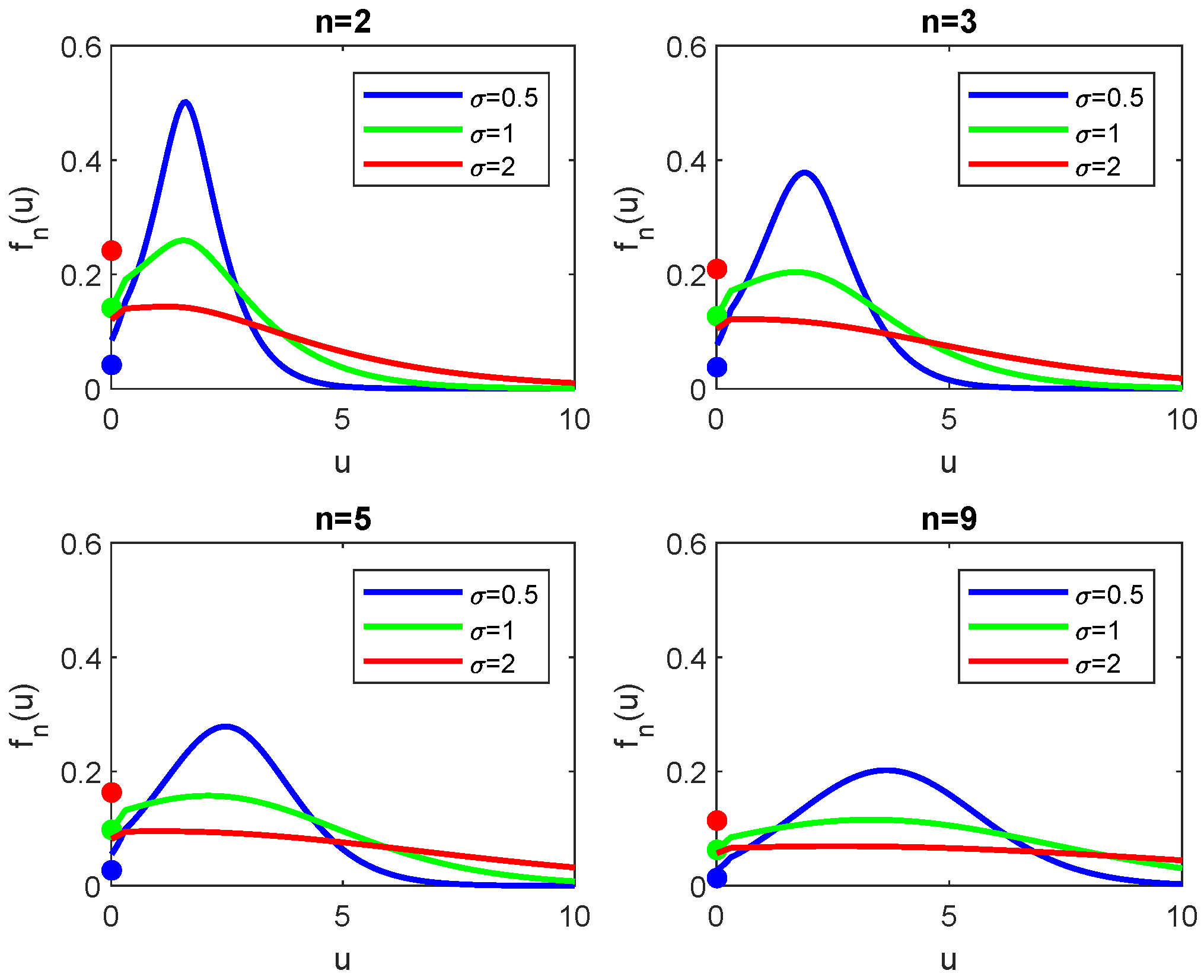
In Figure 2, the density functions of the Lindley process with $\mu =0.3$ and starting position $x=1$ for different values of n and $\sigma$ is shown. We can see that as n increases, the density flattens out, the variance increases, and the maximum of the density moves toward higher values. As $\sigma$ increases, the density flattens out but keeps the position of the maximum. The discrete part of the distribution, represented by a colored dot on the y-axis decreases as n increases. Note also that only when $\sigma =1$ we observe the continuity between the continuous and discrete part of the density; this is due to Corollary 1.

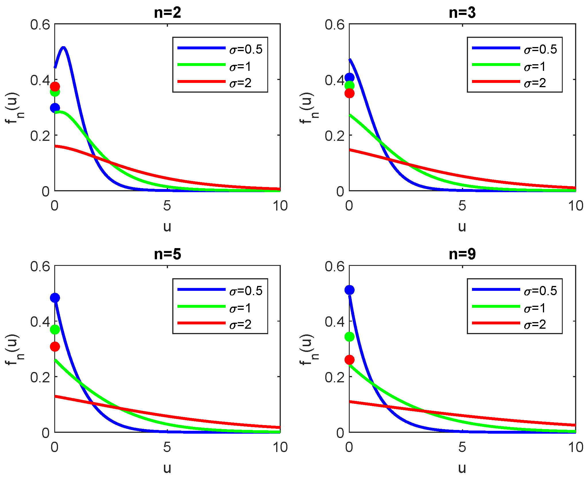
A different behavior appears when the shift term $\mu$ is negative. In Figure 3 the density functions of the Lindley process with the same parameters of Figure 2 and $\mu =-0.3$ is shown. We can see that, as n increases, the density converges to a stationary distribution, as expected from the theory. The interesting remark is that such convergence appears for reasonable small values of n. Please note that the convergence to the steady-state distribution is faster for larger values of $\sigma$. Furthermore, as $\sigma$ increases, the density flattens out, and the variance of $W_n$ increases, as expected since we increased the variability of the process.

Figure 4 shows the density function of the Lindley process with $\sigma =1$, starting position $x=1$ for different values of n and $\mu$. We notice that if $\mu$ is positive, the increase of $\mu$ determines a very similar shape of the density but shifted while, if $\mu$ is negative, as $\mu$ decreases, the density concentrates more and more in zero. Another interesting feature concerns the mass in $u=0$. For positive $\mu$, it decreases as $\mu$ increases. Indeed, the trajectories move quickly away from zero. However, for negative $\mu$, we observe the opposite behavior due to the fact that the trajectories are pushed towards zero, and it becomes increasingly difficult to leave zero. Recall that $\mu <0$ implies the existence of the steady-state distribution. We underline that such distribution is attained faster as $\mu$ decreases.

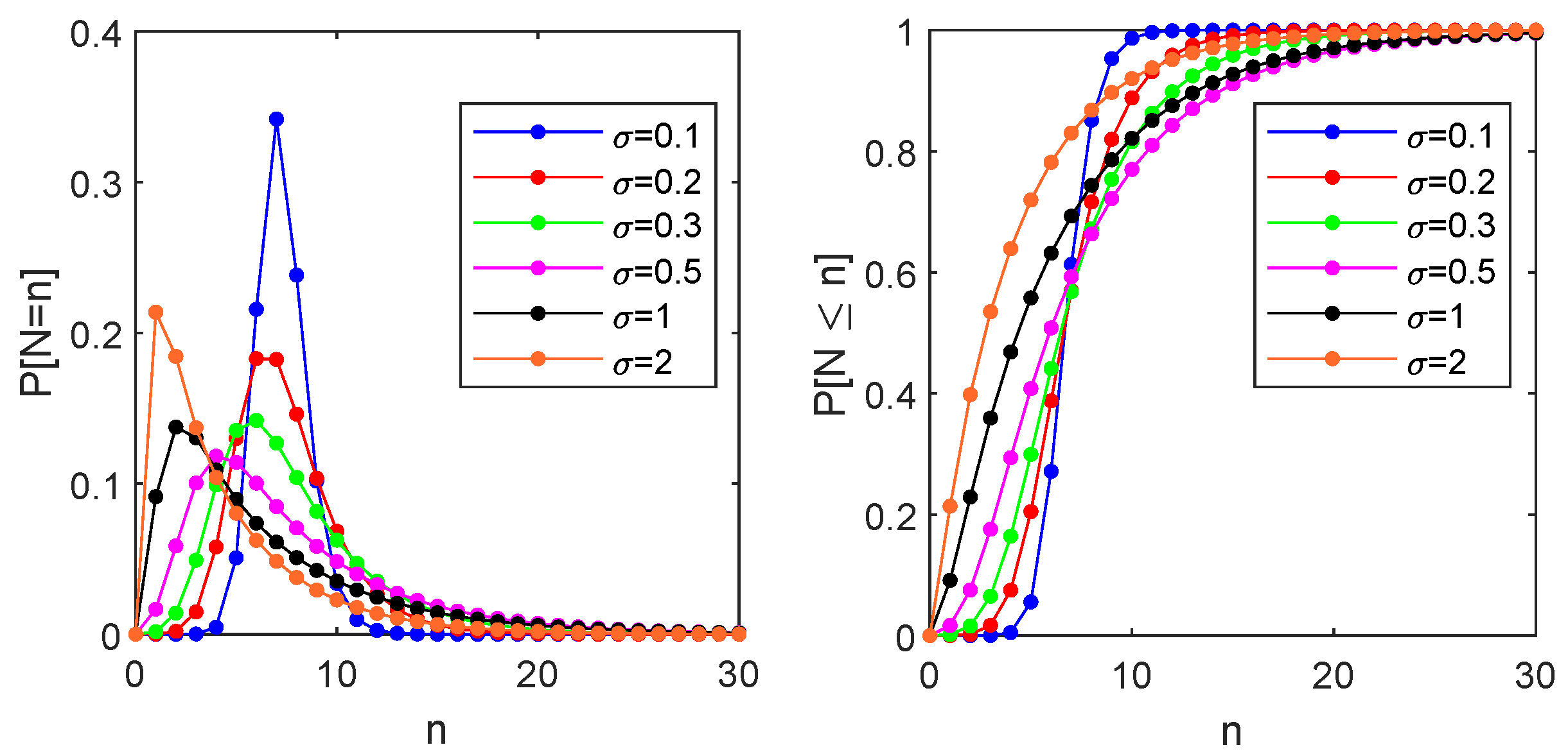
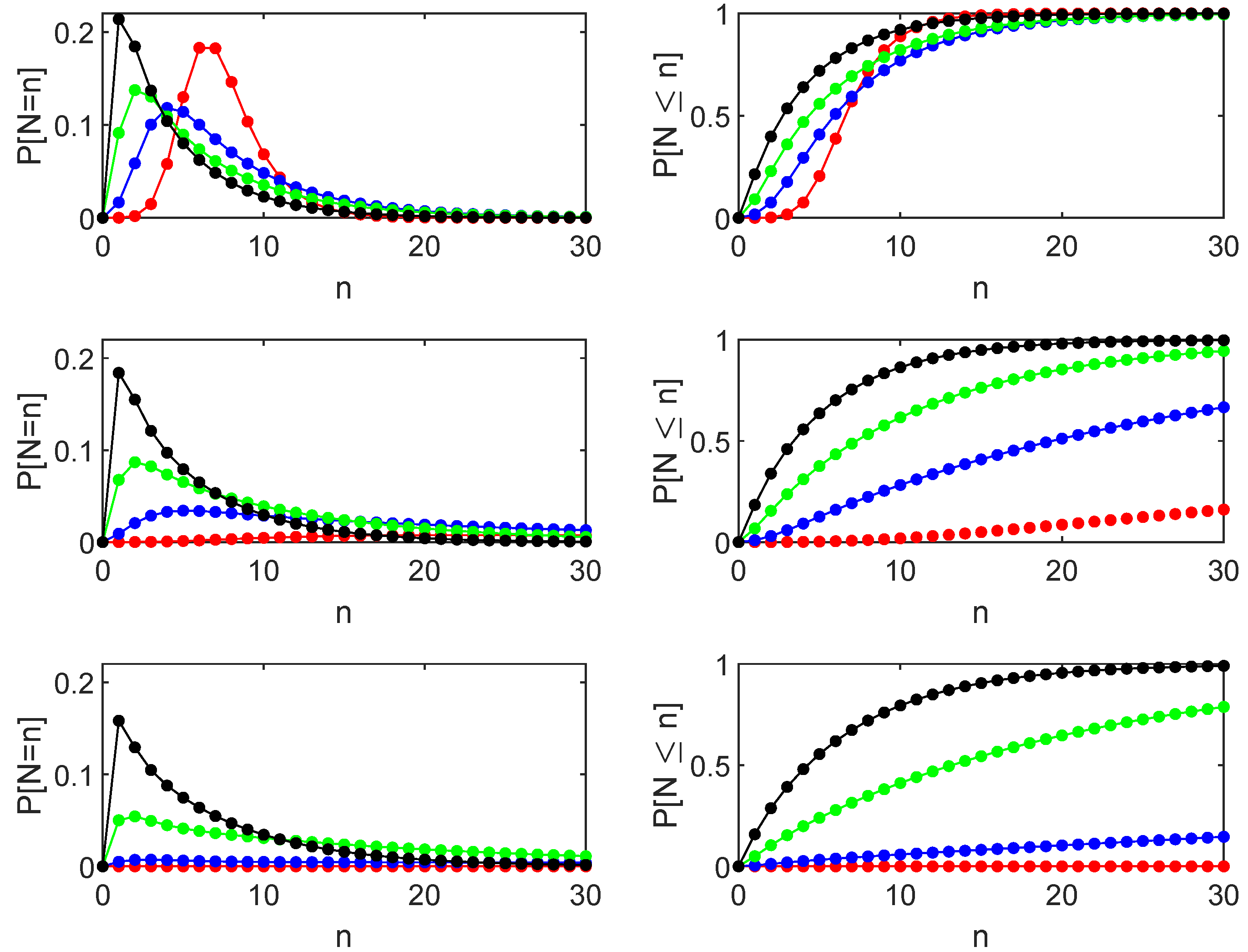
As far as the FET $N_x$ are concerned, in Figure 5, we illustrate the behavior of the probability distribution function $P\left(n\right|x)$ and of its cumulative with starting position $x=1$, boundary $h=3$, $\mu =0.3$ and for different values of $\sigma$. We see a different behavior for small or large values of the dispersion parameter $\sigma$. Indeed, when $\sigma \le 0.5$, $P\left(n\right|x=1)$ has a maximum whose ordinate decreases as $\sigma$ increases while it increases when $\sigma >0.5$. This behavior has an immediate interpretation by observing that almost deterministic crossings determine a high peak when $\sigma$ is small; as far as $\sigma$ increases, the variability of the increments facilitates the crossing that also happens for smaller times, and the probabilistic mass starts to increase sooner.

In Figure 6, we investigate how this behavior evolves when $\mu$ decreases. In particular, we compare the shapes for different values of $\mu =[-0.3,0,0.3]$. Observe that the abscissa of the maximum of the distribution decreases as $\sigma$ increases. Concerning the corresponding ordinate, we observe different behaviors depending on the sign of the parameter $\mu$. Indeed, for positive $\mu$, we have the features already noted in Figure 5. These features are no longer observed when $\mu \le 0$ because here, the deterministic crossing is no longer possible, and crossings are determined only by the noise.

7. An Application: CUSUM with Laplace-Distributed Scores

A problem in reliability theory concerns the change detection of a machinery’s performance. A widely used technique for this aim is known as CUSUM [15,36,37]. In this context, given the observation of a sequence of independent random variables $X_n$, with a probability density function that changes at an unknown Time m:

$$X_n\sim \left\{\begin{array}{c}f\left(x\right),\mathrm{if}1\le n<m\hfill \\ g\left(x\right),\mathrm{if}n\ge m,\hfill \end{array}\right.$$

the method aims to recognize the unknown Time m in which such sequence changes its distribution.

In his pioneering paper [15], Page proposes the CUSUM procedure as a series of Sequential Probability Ratio Tests (SPRTs) between two simple hypotheses, with thresholds of 0 and h. The detection of a change is achieved through repeated application of the likelihood ratio test. Page shows that the likelihood ratio test can be written in an iterative form as (1), where $Z_n$ corresponds to the instantaneous loglikelihood ratio at Time n

$$Z_n=log\left({\displaystyle \frac{g\left(X_n\right)}{f\left(X_n\right)}}\right)$$

(77)

and the stopping time of the test is

$$N^h=inf\{n\ge 1|W_n\notin (0,h)\}.$$

Generally, hypothesis tests involve comparing two alternative values of one distribution parameter. Unfortunately, in most cases, closed-form expressions for the distribution of $Z_n$ are not available. In particular, when parameter changes result in a shift from a symmetric to an asymmetric distribution, it cannot be computed in closed form. However, the results from previous sections allow us to study the case where $f\left(x\right)$ is the Laplace density function (2) and $g\left(x\right)=f\left(x\right)e^{\theta x-b\left(\theta \right)}$, where

$$b\left(\theta \right)=log\left(\mathbb{E}\left[e^{\theta X}\right]\right)=\mu \theta -log(1-{\sigma }^2{\theta }^2)$$

(78)

with $X\sim f\left(x\right)$ and $0<\theta <1/\sigma$. In other words, we suppose that up to Time m, the random variable $X_n$ follows a Laplace distribution $X_n\sim Laplace(\mu ,\sigma )$ with mean $\mu$ while, after Time m, it switches to a skewed Laplace distribution with mean $\mu +\left(2{\sigma }^2\theta \right)/(1-{\sigma }^2{\theta }^2)>\mu$ (cf. Figure 7). Please note that this special case where $f\left(x\right)$ is the Laplace density function (2) is relevant in applications [38]. In this instance, the instantaneous loglikelihood ratio of the n-th observation is

$$Z_n=\theta X_n-b\left(\theta \right),$$

(79)

i.e., it is a linear function of $X_n$ with slope $\theta$ and specific intercept (78) for each slope. The distribution of the loglikelihood ratio is then a rescaled and shifted Laplace random variable $X_n\sim Laplace(\theta \mu -b\left(\theta \right),\sigma \theta )$.

Typically, the value of the boundary h is determined using the average time interval between anomalies, estimated by the experimenter. However, this procedure highly depends on such subjective estimation that does not allow the fixing of Type I error rate $\alpha$.

Here, we propose an alternative algorithm based on the previous section’s results that allows the creation of a test involving the Type I error rate $\alpha$. We fix $\alpha$, and we consider a sequence of SPRTs: in each step $k\ge 1$, we determine the boundary value $h_k^{*}$ such that

$$\mathbb{P}(N^{h_k^{*}}\le k)=\alpha .$$

(80)

In this way, for the k-th SPRT test, we determine a constant boundary $h_k^{*}$ that holds up to Time k.

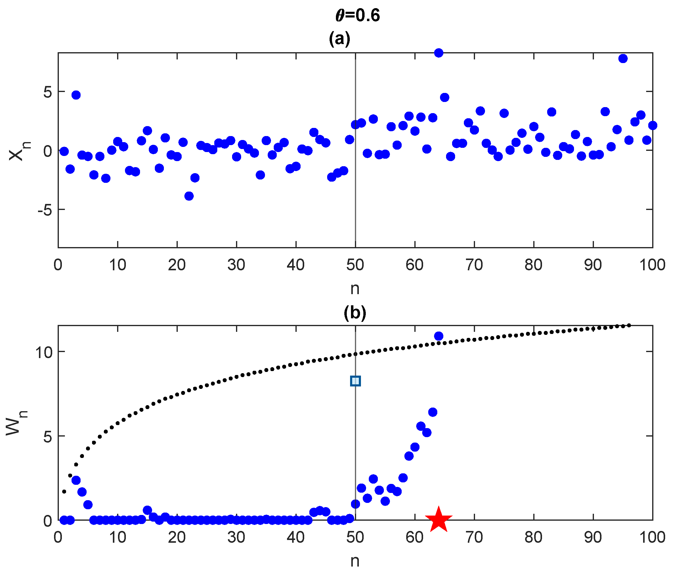
In Figure 8, we simulate data from Laplace distribution with parameters $\mu =0$, $\sigma =1$, $x=0$ and time change $m=50$, i.e., for $n<50$ the parameter $\theta$ is null and for $n\ge 50$ we select $\theta =0.6$. Applying the CUSUM algorithm with the boundary evaluated through (80) we obtain a detection time = 64 (red star in the figure). Looking at the trajectory $X_n$, it is very hard to detect a change time but the test works properly, though with a slight delay in detection.

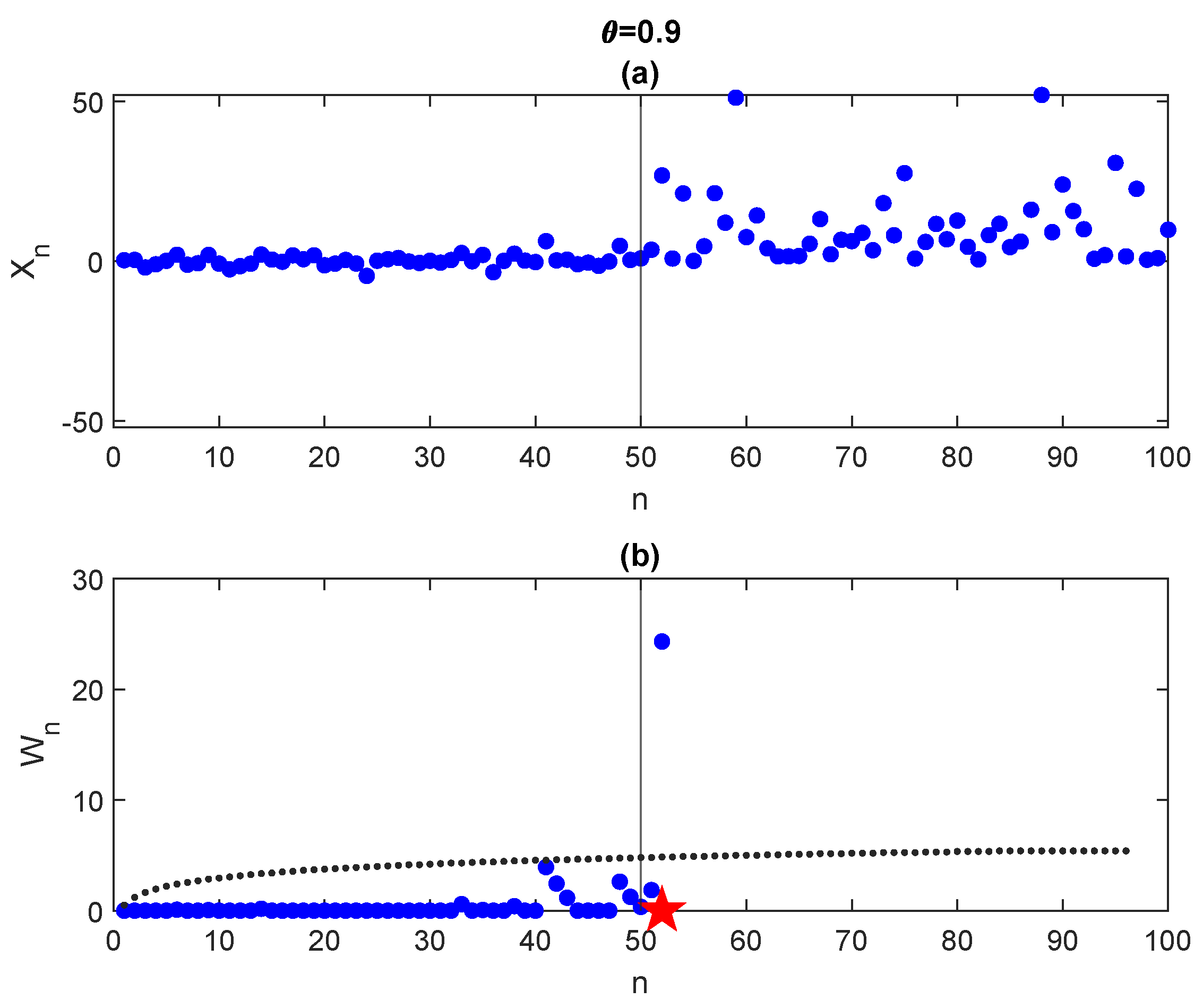
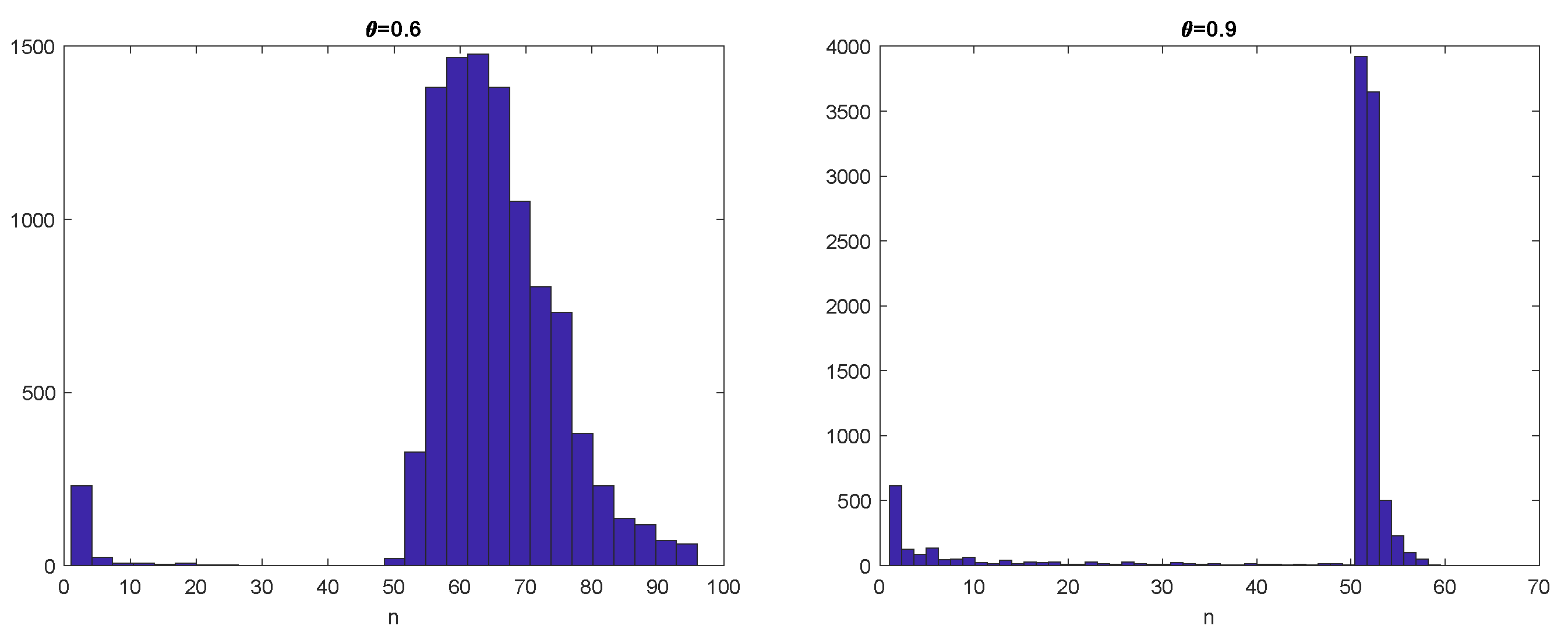
In Figure 9, we perform the same experiment but with $\theta =0.9$. Applying the CUSUM algorithm with the corresponding boundary, we obtain a detection time = 52 (red star in the figure). As expected, as $\theta$ increases, the detection becomes easier and more precise. This is confirmed in Figure 10 where histograms of the first exit time when $\theta =0.6$ (left) and $\theta =0.9$ (right) are shown for a sample of ${10}^4$ trajectories.

8. Conclusions

We derived recursive formulae for the distributions of both the position and the first passage time through a constant boundary of a Lindley process with Laplace-distributed increments. The existence of these formulae enabled us to develop the necessary computational software, which is available on GitHub. Our approach heavily relies on the ability to obtain recursive formulae for the involved integrals. It is mainly possible by the presence of exponentials in the increment distribution. Unfortunately, this advantage limits the immediate generalization of our method to different distributions or boundaries, while the case of a multidimensional Lindley process could be tractable but would be highly demanding in terms of the complexity of the involved formulae. Nonetheless, the Laplace distribution plays a significant role in the CUSUM framework and queuing theory. Future research could further explore these applications, potentially addressing related estimation problems in reliability. Additionally, it would be interesting to compare the performance of other change point detection methods and investigate the applicability of the presented results within the context of queuing models.