A Non-Parametric Test for a Two-Way Analysis of Variance

Abstract

The methodology carried out in this work is based on non-parametric inference. The problem is framed as a regression analysis, and the solution is derived using the permutation approach. The proposed test does not rely on the assumption that the distribution of the response follows a specific family of probability laws, unlike other parametric approaches. This makes the test powerful, particularly when the typical assumptions of parametric approaches, such as the normality of data, are not satisfied and parametric tests are not reliable. Furthermore, this method is more flexible and robust with respect to parametric tests. A permutation test on the goodness-of-fit of a multiple regression model is applied. Hence, proposed solution consists of the application of permutation tests on the significance of the single coefficients and then a combined permutation test (CPT) to solve the overall goodness-of-fit testing problem. Furthermore, a Monte Carlo simulation study was performed to evaluate the power of the previously mentioned permutation approach, comparing it with the conventional parametric F-test for ANOVA and the bootstrap combined test, both commonly discussed in the literature on this statistical problem. Finally, the proposed non-parametric test was applied to real-world data to investigate the impact of age and smoking habits on medical insurance costs in the USA. The findings suggest that smoking and being at least 50 years old significantly contribute to increased medical insurance costs.

1. Introduction

The paper deals with a two-way analysis of variance, in the presence of two two-level factors and a numeric response. The motivating example of this work concerns the US population’s medical insurance cost, and the effect on it of age and being a smoker. Recently, the actuarial modelling of insurance claims has emerged as a significant research topic in the health insurance industry and is primarily used for establishing appropriate premiums [1]. This is crucial for enticing and keeping insured individuals, as well as for effectively managing current plan members. Nevertheless, because of the numerous elements influencing medical insurance expenses and the complexities involved, there are challenges in precisely developing a predictive model for it. Elements such as demographic data, health conditions, access to healthcare based on location, lifestyle habits, and characteristics of providers can significantly influence the anticipated expenses of medical insurance. Additional important aspects such as the extent of coverage, the kind of plan, the deductible amount, and the customer’s age at the time of enrollment also significantly influence the possible expenses associated with medical insurance [2].

In some countries, such as the United States, it is nowadays essential for the population to have health insurance [3,4]. One of the largest yearly expenses individuals face is their health insurance coverage. Health insurance represents a third of the GDP, and medical care is necessary for everyone at different levels. Shifts in medical practices, trends in pharmaceuticals, and political influences are just some of the numerous factors that create yearly variations in healthcare expenses [5]. Some research indicates that insurance companies ought to adjust their policies based on the smoking habits, BMI, and age of their clients in order to offer insurance plans that cater to the public’s needs [6].

Grasping the factors that impact an individual’s health insurance premium is essential for insurance companies to set appropriate prices. When making informed decisions, the premium should always be the primary focus for users. Several empirical works in the literature investigate the main factors that significantly correlate with health insurance costs. Charges are positively related to smoking and age. The importance of health insurance is growing as individuals’ lifestyles and health issues evolve. Since a medical condition can affect anyone unexpectedly and can have significant psychological and financial repercussions, it is challenging to determine when these issues will arise. Given this context, some authors [7] aimed to predict health insurance costs based on the following factors: age, sex, geographical location, smoking status, body mass index (BMI), and number of children [8,9]. Age, BMI, chronic diseases, and family history of cancer have been shown to be the most influential factors determining the premium price [10,11].

One of the goals of the paper is that the empirical findings of this study will assist policymakers, insurers, and prospective medical insurance purchasers in making informed choices about selecting policies that fit their individual requirements. To study the effect of age and smoking on insurance costs, we use sample data. The problem under study can be traced back to a two-way ANOVA layout. We are interested in testing the significance of both the main effect of each factor and the interaction between the two. Some solutions have been carried out in the methodological literature for the ANOVA problem. Some researchers have examined the two-way ANOVA model with varying cell frequencies without assuming equal error variances. By employing a generalized approach to calculate p-values, the traditional F-tests on the interaction and main effects are expanded to accommodate heteroscedasticity. The generalized F-tests introduced in the aforementioned study can be applied in significance testing or in fixed level testing according to the Neyman–Pearson framework. Simulation studies reveal that, although the method shows enhanced power in the presence of heteroscedasticity, the size of the test does not surpass the predetermined significance level [12]. Another work states that determining the a priori power for univariate repeated measures (RM) ANOVA designs with two or more factors is currently difficult due to the lack of accurate methods for estimating the error variances used in power calculations. Hence, Monte Carlo simulation procedures have been used to estimate power under different experimental conditions [13]. The main problem remains that this method provides only an estimate and not an adequate procedure for the statistical problem. In another study by Toothaker and Newman (1994) [14], the ANOVA F-test and several non-parametric competitors for two-way design were compared in terms of empirical $\alpha$ and power. Through a simulation study, they confirmed that the ANOVA F-test suffers from conservative $\alpha$ and power for the mixed normal distribution.

As said, in this work, the goal is to investigate the main and interaction effects of crucial factors, such as being a smoker (yes or no) and age (less than 50 years old and greater than or equal to 50 years old) in an experimental framework where the response variable is the charges of medical insurance costs. The proposed methodological approach is based on a non-parametric inference. The problem is framed within the context of a regression analysis, and the resolution relies on a permutation method. The suggested test, in contrast to parametric methods, does not necessitate the assumption that the response distribution adheres to a particular set of probability distributions. This type of test is highly effective, particularly when the usual assumptions of parametric methods (like data normality) are unmet and the validity of parametric tests is compromised [15]. Moreover, the proposed approach demonstrates greater flexibility and robustness compared to parametric tests, and it can be viewed in opposition to stepwise regression [16]. Actually, it is based on a permutation test to evaluate the goodness-of-fit of a multiple regression model. This solution is based on a multiple testing approach, that jointly assesses the significance of all single regression coefficients, including both main effects and interaction effects. The method consists of combining the p-values of the partial tests on the regression coefficients. The approach of combined permutation tests has been effectively implemented across various contexts [17,18]. In particular, it has been widely applied in empirical studies [19], with numeric variables but also categorical data [20], for big data problems [21], in regression analysis [22,23], to test directional and non-monotonic hypotheses [24,25], with count data [24] and in many other problems.

Permutation goodness-of-fit assessments, using partial sums or cumulative sums of residuals, have been suggested for linear regression models [26]. In order to evaluate the influence of covariates, the authors of [27] introduced the concept of combining non-parametric permutation tests. The notion of treating the test for the validity of a multivariate linear model as a simultaneous test was put forward by [28] within the context of rotation tests. Moreover, in the literature, several recent articles discuss approaches for assessing goodness-of-fit through the permutation approach in linear regression models, as well as the use of non-parametric permutation tests to evaluate the influence of covariates. For instance, ref. [29] proposes a non-parametric test to assess the effect of covariates on the cure rate in mixture cure models, employing a bootstrap method to approximate the null distribution of the test statistic. On the other hand, a previous study generalizes the metric-based permutation test for the equality of covariance operators to multiple samples of functional data, utilizing a non-parametric combination methodology to merge pairwise comparisons into a global test [30].

The rest of the paper is organized as follows. Section 2 presents the statistical problem. The methodological proposed solution is explained in Section 3. Section 4 contains the Monte Carlo simulation study. The case study is described in Section 5 and Section 6 includes the overall conclusions.

2. Statistical Problem

Let us consider a model with binary variables as predictors, to represent the main effects and the interaction effects of two factors with two levels. This situation was first considered by [31] because it is typical of experimental designs where subjects are first divided into homogeneous subgroups (blocks) and then randomly assigned to various treatment levels. Under the null hypothesis, all the treatment effects are null. On the other hand, in the alternative hypothesis, at least one effect is not equal to zero.

Let $x_{kji}$ denote the i-th observation of the response variable related to the combination of levels $(k,j)$, that is the value observed on the i-th unit (i-th replication) when factor 1 is at level k and factor 2 is at level j ($k=1,\dots ,K$; $j=1,\dots ,C$). Data are assumed to be realizations of random variables $X_{kji}$ which behave according to the following linear model:

$$X_{kji}=\mu +{\theta }_k+{\gamma }_j+{\left(\theta \gamma \right)}_{kj}+{\epsilon }_{kji},$$

(1)

where ${\theta }_k$ and ${\gamma }_j$ are the main effects of factor 1 at level k and factor 2 at level j, respectively, ${\left(\theta \gamma \right)}_{kj}$ is the interaction effect related to factor 1 at level k and factor 2 at level j and ${\epsilon }_{kji}$ are exchangeable errors, with zero mean and unknown continuous distribution [15]. In this situation, without loss of generality, for ease of interpretation, it is also possible to consider the usual constraints:

$$\sum _{k=1}^K{\theta }_k=0,\sum _{j=1}^C{\gamma }_j=0,\sum _{k=1}^K{\left(\theta \gamma \right)}_{kj}=0\forall j,\sum _{j=1}^C{\left(\theta \gamma \right)}_{kj}=0\forall k.$$

(2)

Typically, three potential testing problems could be examined independently:

• $H_{0\theta }:\left[{\theta }_k=0\mathrm{for}\mathrm{every}k\right]$, against $H_{1\theta }:\left[{\theta }_k\ne 0\mathrm{for}\mathrm{some}k\right]$ (significance of main effect of factor 1);
• $H_{0\gamma }:\left[{\gamma }_j=0\mathrm{for}\mathrm{every}j\right]$, against $H_{1\gamma }:\left[{\gamma }_j\ne 0\mathrm{for}\mathrm{some}j\right]$ (significance of main effect of factor 2);
• $H_{0\theta \gamma }:\left[{\left(\theta \gamma \right)}_{kj}=0\mathrm{for}\mathrm{every}(k,j)\right]$, against $H_{1\theta \gamma }:\left[{\left(\theta \gamma \right)}_{kj}\ne 0\mathrm{for}\mathrm{some}(k,j)\right]$ (significance of interaction effect).

Under the null hypothesis related to one of the three problems, exchangeability is applicable only among certain data blocks (determined by the $C\times K$ combinations of levels), and thus only synchronized permutations are permitted [32]. For instance, if we want to compare two treatments of factor 1, corresponding to levels $k_1$ and $k_2$ of the factor, where $1\le k_1<k_2\le K$, we can shuffle data between blocks having the same level of factor 2, one featuring factor 1 at level $k_1$ and the other at level $k_2$. In other words, by representing the data block with $(k,j)$ as having factor 1 at level k and factor 2 at level j, we can interchange data between $(k_1,j)$ and $(k_2,j)$ for each j, ensuring that the permutations between the C pairs of blocks remain synchronized. These synchronized permutations are a valid alternative because it is among the permutation methods used for the two-way (M)ANOVA. However, this method only works when the aim is to test only one factor and consider the others as confounders. This is different from our proposal because we want to verify the significance of the estimates of all the single coefficients jointly considered.

The data can be alternatively represented using a different notation. Let $y_1,y_2,\dots ,y_n$ be the observed data of the response, where n is the total number of observations and $y_i$ is the i-th observation of the response, with $i=1,\dots ,n$. If we consider the case of two factors at two levels, i.e., $K=C=2$, and assume $y_i$ to be a realization of the random variable $Y_i$, an alternative linear model in the framework of the linear regression analysis is the following:

$$Y_i={\beta }_0+{\beta }_1{D}_{i1}+{\beta }_2{D}_{i2}+{\beta }_{12}{D}_{i1}{D}_{i2}+{\epsilon }_i,$$

(3)

where $D_{iv}$ is a dummy variable that takes the value 0 if the i-th observation is associated to the v-th factor at level 1, and takes the value 1 if the i-th observation is related to the v-th factor at level 2, with $i=1,\dots ,n$ and $v=1,2$. In the regression model, ${\epsilon }_1,\dots ,{\epsilon }_n$ are exchangeable random errors and ${\beta }_0,{\beta }_1,{\beta }_2,{\beta }_{12}$ are unknown parameters, with ${\beta }_0$ as the expected value of the response corresponding to the baseline (both the factors at level 1), ${\beta }_1$ and ${\beta }_2$ as the main effects of factor 1 and factor 2, respectively, and ${\beta }_{12}$ as the interaction effect.

3. Permutation Solution

Regarding the regression coefficients of the reparameterized model (3), we are interested in the following system of hypotheses:

$$\left\{\begin{array}{cc}{H}_0:\hfill & {\beta }_1={\beta }_2={\beta }_{12}=0\hfill \\ H_1:\hfill & \overline{H_0}\hfill \end{array}\right..$$

(4)

Given that we aim to determine which coefficients have significant estimates when the null hypothesis is rejected, our approach involves conducting multiple tests to assess the significance of the single regression coefficients. A solution to the aforementioned statistical problem concerns the use of a combined permutation test (CPT) [33]. The overall testing problem can be considered a multiple test, composed by the partial tests on the significance of the regression coefficients’ estimates [34].

The system of hypotheses of the partial test concerning the main effect of the vth factor is

$$\left\{\begin{array}{c}{H}_0^v:{\beta }_v=0\hfill \\ H_1^v:{\beta }_v\ne 0\hfill \end{array}\right.$$

with $v=1,2$. Similarly, the system of hypotheses of the partial test concerning the interaction effect of the two factors is

$$\left\{\begin{array}{c}{H}_0^{12}:{\beta }_{12}=0\hfill \\ H_1^{12}:{\beta }_{12}\ne 0.\hfill \end{array}\right.$$

Therefore, the null and alternative hypotheses of the overall problem can be represented as follows:

$$\left\{\begin{array}{cc}{H}_0:\hfill & H_0^1\bigcap H_0^2\bigcap H_0^{12}\hfill \\ H_1:\hfill & H_1^1\bigcup H_1^2\bigcup H_1^{12},\hfill \end{array}\right.$$

(5)

where the intersection symbols mean that all the partial null hypotheses are true under $H_0$, and the union symbols indicate that, under $H_1$, at least one partial alternative hypothesis is true.

The proposed solution consists of the application of permutation tests on the significance of the single coefficients and then a CPT to solve the overall testing problem by combining the inferential results of the partial tests. Reasonable test statistics for the partial tests on the single coefficients are the absolute values of suitable estimators of the parameters. Formally, an appropriate partial test statistic for the main effect of the vth factor is

$$T_v=\left|{\widehat{\beta }}_v\right|$$

with $v=1,2$. Therefore, a suitable partial test statistic for the interaction effect is

$$T_{12}=\left|{\widehat{\beta }}_{12}\right|.$$

The null distribution of the test statistics is obtained by permuting the rows of the design matrix, keeping the vector of observed values of the response fixed, and recalculating for each permutation the estimates of the coefficients and, consequently, the values of the test statistics. This non-parametric method is very useful for solving complex problems and the main advantage with respect to parametric methods is that the multivariate distribution of the trivariate test statistic does not need to be known, and in particular, the dependence structure between variables does not need to be explicitly modelled or specified [35]. Permutation tests are distribution-free, hence they are flexible and robust with respect to the departure from normality [32].

The core concept of a combined permutation test is to identify an appropriate statistic for each partial test and to aggregate the permutation p-values from these tests to address the overall problem [33]. In our case, the absolute values of the least squares estimators of the regression coefficients serve as suitable and effective test statistics for the partial tests. The procedure follows these steps:

• Computation of the vector of observed values of the test statistics $T_0=\left\{\right|b_1|,|b_2|,|b_{12}\left|\right\}=T\left(X\right)$;
• B independent random permutations of the rows of the X matrix: $X_1^{*},X_2^{*},\dots ,X_B^{*}$;
• Computation of the values of the test statistic vector for the B dataset permutations $T_b^{*}$ and the corresponding vector of p-values ${\lambda }_b^{*}$ with $b=1,2,\dots ,B$;
• Computation of the value of the combined test statistic for each permutation and for the observed dataset through the combination of the partial p-values with a suitable function $\psi$: $T_{\mathrm{comb}}=\psi \left({\lambda }_b^{*}\right)$;
• Computation of the p-value of the combined test according to the null permutation distribution.

The dependence of the partial tests is implicitly taken into account through the permutation of the rows of the design matrix. Since each partial null hypothesis is rejected for large values of the test statistic, without loss of generality, we assume the same rejection rule for the combined test statistic of the overall problem. Therefore, a suitable combined test statistic $\psi$ is:

$$T_{\mathrm{comb}}=-2\sum _{j}ln\left({\lambda }_j\right)=-2·\left[ln\left({\lambda }_1\right)+ln\left({\lambda }_2\right)+ln\left({\lambda }_{12}\right)\right],$$

(6)

where ${\lambda }_1$, ${\lambda }_2$ and ${\lambda }_{12}$ are the p-values of the partial tests. Equation (6) represents Fisher’s combination function which, among the various combination functions available in the literature, exhibits a good power behavior regardless of the proportion of true partial alternative hypothesis [36,37]. Since such a permutation ANOVA for the linear regression models is defined as a multiple tests, in the case of a rejection of the null hypothesis in favor of the alternative and, in order to attribute the overall significance to specific partial tests (i.e., to specific coefficient estimates), the control of the family-wise error (FWE) is necessary [38,39]. Family-wise error rate (FWE) refers to the probability of making at least one type I error (false positive) when performing multiple statistical tests on the same dataset [40]. It is a key concept in multiple comparisons and hypothesis testing, particularly when testing multiple hypotheses simultaneously. When conducting multiple statistical tests, the likelihood of incorrectly rejecting at least one true null hypothesis (type I error) increases. In other words, to avoid the inflation of the type I error of the overall test, we must adjust the partial p-values. A suitable method is the one based on the Bonferroni–Holm rule [41]. This correction procedure works as follows. Given a set of m partial p-values:

• all p-values are sorted in order of smallest to largest;
• if the smallest p-value is greater than or equal to $\alpha /m$, the procedure is stopped and no p-value must be considered significant. Otherwise, go to step three;
• the smallest p-value is considered significant, then the second smallest p-value is compared to $\alpha /(m-1)$. If the second smallest p-value is greater than or equal to $\alpha /(m-1)$, the procedure is stopped and no other p-value is considered significant. Otherwise, go to step four;
• repeat steps 2 and 3 on the remaining p-values until you find the first non-significance.

The method’s application to the real data of the case study, along with the simulation analysis, was conducted using original R scripts developed by the authors. Actually, for the regression model, the R function lm() was carried out. The graphs were created with the corresponding R functions plot(), hist() and boxplot().

4. Monte Carlo Simulation Study

A Monte Carlo simulation analysis was conducted to assess the power behavior of the non-parametric test discussed in the paper (CPT) in comparison to the traditional parametric F-test for the ANOVA and to the bootstrap combined test (TBC), also present in the literature concerning this statistical problem. The previously mentioned competitor, TBC, was implemented by taking inspiration from the technique reported in [42,43]. In practice, this method, unlike CPT, generates the B simulated datasets by resampling the original data with replacement. Once the bootstrapped datasets are generated, the technique for combining the partial p-values, related to the significance of the individual regression coefficients, remains the same as in the CPT procedure.

Let n and q denote the sample size and the number of binary factors of the model, respectively (in our specific case $q=2$). The binary data were simulated by randomly generating values from normal distributions and then transforming such values into binary data. Specifically, $n\times q$ matrix $\mathbf{Z}$ was simulated by randomly generating n observations from a q-variate normal distribution with null mean vector and variance–covariance matrix $\mathbf{\Sigma }$, i.e., $\mathbf{Z}\sim {\mathcal{N}}_q({\mathbf{0}}_{\mathbf{q}},\mathbf{\Sigma })$. We assumed that the variance of each component of the underlying bivariate normal distribution was constant and equal to ${\sigma }_z^2$ and the correlation between each couple of components ${\rho }_z$. Consequently, $\mathbf{\Sigma }={\sigma }_z^2[{\rho }_z{\mathbf{J}}_{\mathbf{q}}+(1-{\rho }_z){\mathbf{I}}_{\mathbf{q}}]$, where ${\mathbf{J}}_{\mathbf{q}}$ denotes the $q\times q$ all-ones matrix and ${\mathbf{I}}_{\mathbf{q}}$ is the $q\times q$ identity matrix. In our simulations, we set ${\sigma }_z=1$ and ${\rho }_z=0.30$. According to the extensive notation, we have:

$$\mathbf{\Sigma }=\left(\begin{array}{cccc}{\sigma }_z^2& {\sigma }_z^2{\rho }_z& \dots & {\sigma }_z^2{\rho }_z\\ {\sigma }_z^2{\rho }_z& {\sigma }_z^2& \dots & {\sigma }_z^2{\rho }_z\\ ⋮& ⋮& \ddots & ⋮\\ {\sigma }_z^2{\rho }_z& {\sigma }_z^2{\rho }_z& \dots & {\sigma }_z^2\end{array}\right).$$

Then, the model design matrix $\mathbf{X}$ was obtained by transforming the elements of $\mathbf{Z}$ into binary data and adding the column of ones and the products between factors to take into account the constant of the model and the interaction, respectively. As said, we focused on the case $q=2$. Let ${\theta }_1$ and ${\theta }_2$ denote the probability of success (or population proportion of ones) of the underlying Bernoulli random variables corresponding to the first and the second factors, respectively. The binary simulated value $x_{iv}$ corresponding to the ith observation of the vth factor was computed as follows:

$$x_{iv}=I_{(-\infty ,{\Phi }^{-1}\left({\theta }_v\right)]}(z_{iv}/{\sigma }_z),$$

where $I_A(·)$ is the indicator function of the set A, $\Phi (·)$ is the cumulative distribution function of the standard normal distribution, and ${\Phi }^{-1}(·)$ its inverse, that is the Gaussian quantile function, with $v=1,2$. In the simulations, we considered the realistic values ${\theta }_1=0.30$ and ${\theta }_2=0.20$. Hence, the simulated matrix of predictors is the following:

$$\mathbf{X}=\left(\begin{array}{cccc}1& x_{11}& x_{12}& x_{11}{x}_{12}\\ 1& x_{21}& x_{22}& x_{21}{x}_{22}\\ ⋮& ⋮& \ddots & ⋮\\ 1& x_{n1}& x_{n2}& x_{n1}{x}_{n2}\end{array}\right).$$

In order to simulate the values of the numeric response, we assumed three different distributions for the model random errors, mainly to evaluate the effect of the distribution skewness on the inferential results. The n i.i.d. errors, simulated from probability distributions with different skewness, were rescaled to respect a distribution variance of ${\sigma }_{\epsilon }=12$, very similar to that of the case study, and centred on the mean value 0. Let ${\epsilon }_i$ and ${\tilde{\epsilon }}_i$ denote the error randomly generated and the transformed one (rescaled and centered), respectively. The three cases are:

• ${\epsilon }_i\sim \mathcal{N}(0,{\sigma }_{\epsilon }^2)$, i.e., errors generated from a normal distribution, such that $skewness=0$, then ${\tilde{\epsilon }}_i={\epsilon }_i$;
• ${\epsilon }_i\sim {\chi }_{13}^2$, i.e., errors generated from a chi-square distribution with 13 degrees of freedom, such that $skewness=\sqrt{8/13}=0.78$ (moderate asymmetry), then ${\tilde{\epsilon }}_i=({\epsilon }_i-13){\sigma }_{\epsilon }/\sqrt{26}$;
• ${\epsilon }_i\sim {\chi }_2^2$, i.e., errors generated from a chi-square distribution with 2 degrees of freedom, such that $skewness=\sqrt{8/2}=2$ (high asymmetry), then ${\tilde{\epsilon }}_i=({\epsilon }_i-2){\sigma }_{\epsilon }/2$.

The values of the dependent variable were obtained by adding the simulated deterministic part of the model and the transformed simulated errors, according to the regression model reported in Equation (3). Hence, the vector of n simulated values of the response is computed as follows:

$$\tilde{y}=\mathbf{X}\beta +\tilde{\epsilon },$$

where $\tilde{y}={({\tilde{y}}_1,\dots ,{\tilde{y}}_n)}^{\prime }$, $\beta ={({\beta }_0,{\beta }_1,{\beta }_2,{\beta }_{12})}^{\prime }$, and $\tilde{\epsilon }={({\tilde{\epsilon }}_1,\dots ,{\tilde{\epsilon }}_n)}^{\prime }$.

For every simulation setting, the total number of datasets created for power estimation was 1000, and the count of random permutations to establish the null distribution of the test statistics was $B=1000$. The approximation would certainly improve with B = 10,000, which is the choice we made in the case study. Nevertheless, using 1000 permutations in the conditional Monte Carlo method is adequate to achieve a satisfactory level of approximation, ensuring reliable outcomes from the simulations [15,33] and computational efficiency. To address the computational limit of the permutation approach and guarantee both robustness and feasibility of the procedure, either Monte Carlo approximations or parallel computing techniques could be also considered [44,45]. In the simulations, a comparative performance analysis of the CPT method and the classic F-test of the parametric approach was carried out.

The setting parameters which vary in the simulations are the following:

• n is the sample size,
• ${\beta }_0$, ${\beta }_1$, ${\beta }_2$ and ${\beta }_{12}$ are the coefficients of the regression equation.
• $skewness=\sqrt{8/df}$, where $df$ represents the degrees of freedom of the chi-square distribution of errors (→∞ in case of normality)

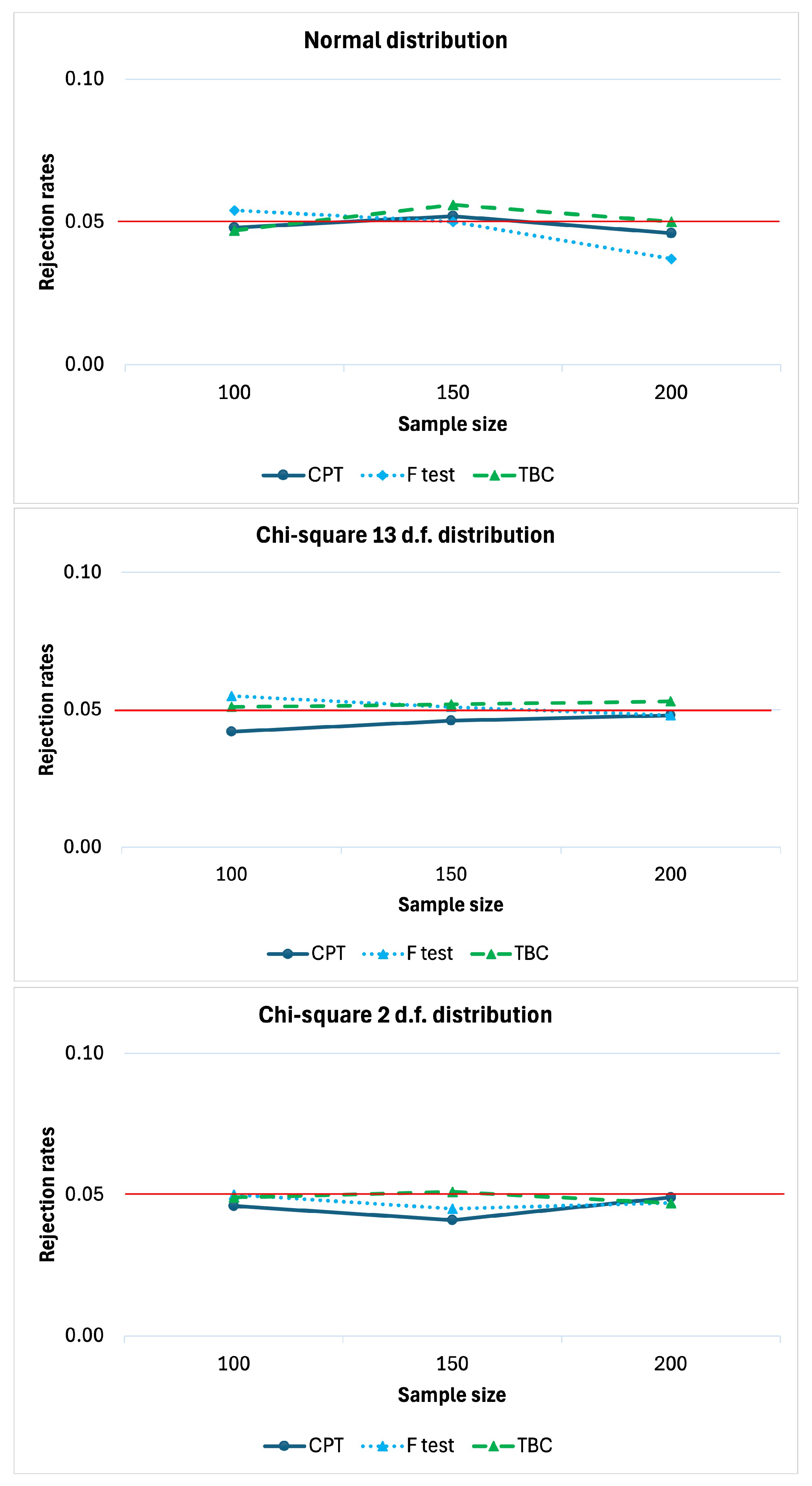
Firstly, simulations were carried out under the null hypothesis ($H_0$), with ${\beta }_0=13$ and ${\beta }_1={\beta }_2={\beta }_{12}=0$. Figure 1 reports the rejection rates of the compared tests as a function of the sample size n. The rejection rate refers to the proportion of times $H_0$ is rejected in a simulation. Indeed, under $H_0$, these values should remain below the predefined significance level $\alpha$ to prove that the tests are well approximated. It is evident that all three tests are well approximated because the rejection rates are all under or very close to the significance level $\alpha =0.05$. Even though the competitor TBC is often above or close to the reference value $\alpha$.

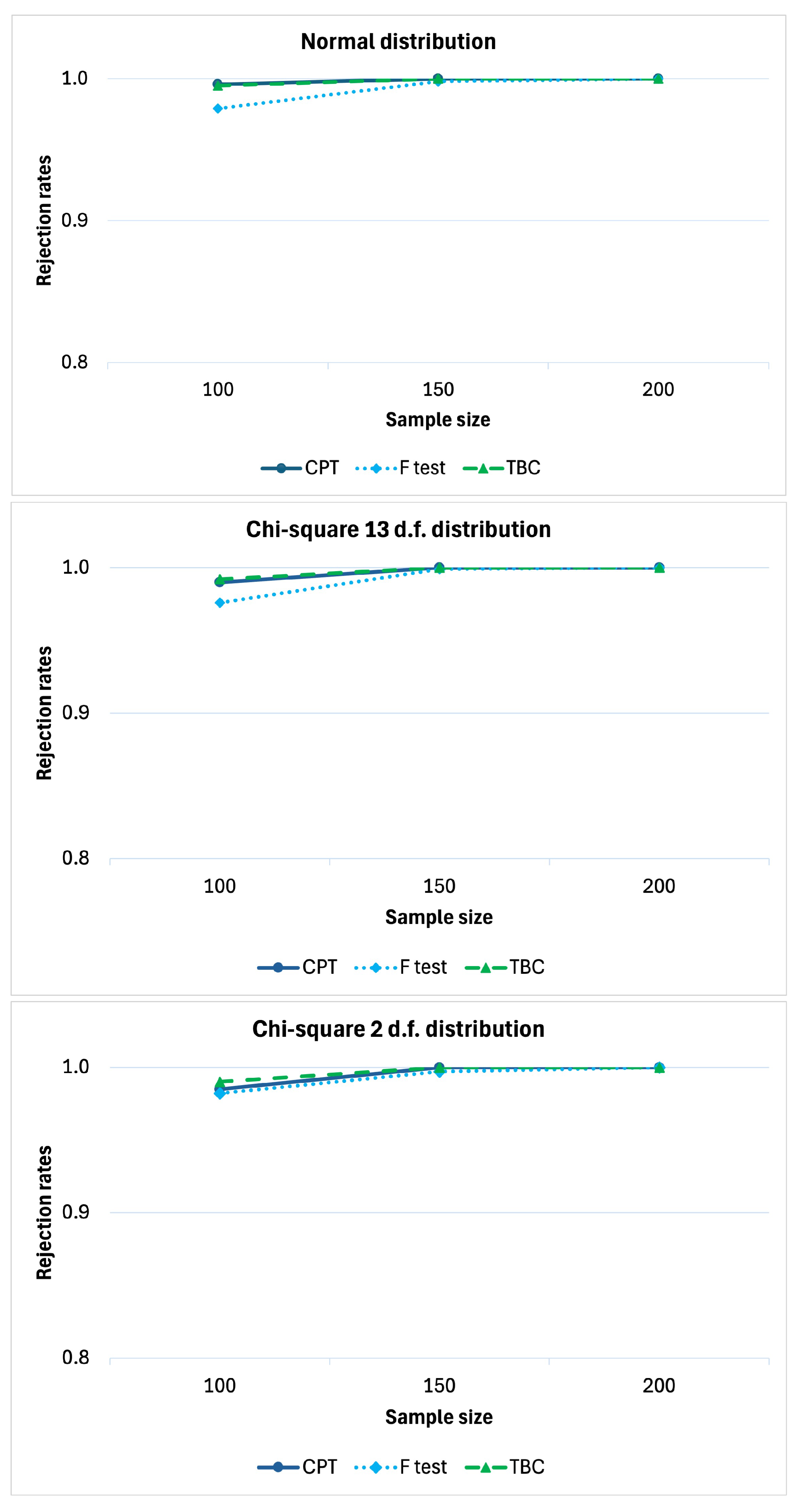
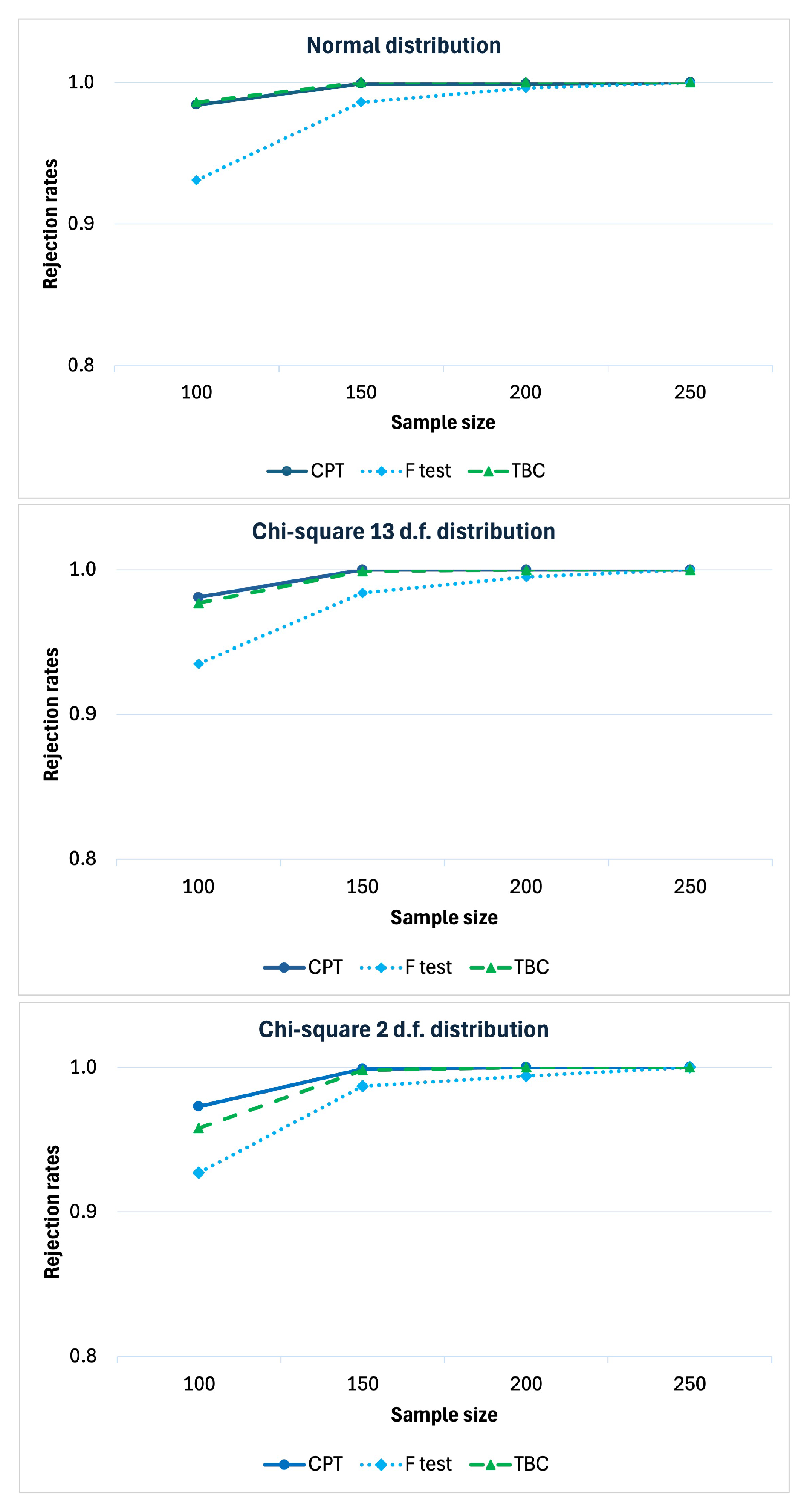
We studied the power behavior under $H_1$ in the scenario with positive main effects of the two factors and null interaction effect, similarly to the empirical results of the case study. The power of a statistical test is the probability of rejecting the null hypothesis when the alternative hypothesis is true. This probability is typically represented by a curve that illustrates the test’s power as a function of sample size, number of partial tests, or other parameters of interest. The power under such a scenario, as a function of the sample size, is reported in Figure 2 to evaluate the consistency of the test. In general, all the three tests are consistent. The power of the proposed method is slightly greater than that of the parametric F-test and also the non-parametric method based on a bootstrap approach (TBC). Furthermore, when n diverges, the proposal tends to infinity faster. We carried out the simulations under the same scenarios except ${\beta }_{12}=10$ (to consider the case of positive interaction effect as well). The results confirm that the CPT is more powerful than the parametric F-test and than the TBC approach. Additionally both of them are consistent (see Appendix A).

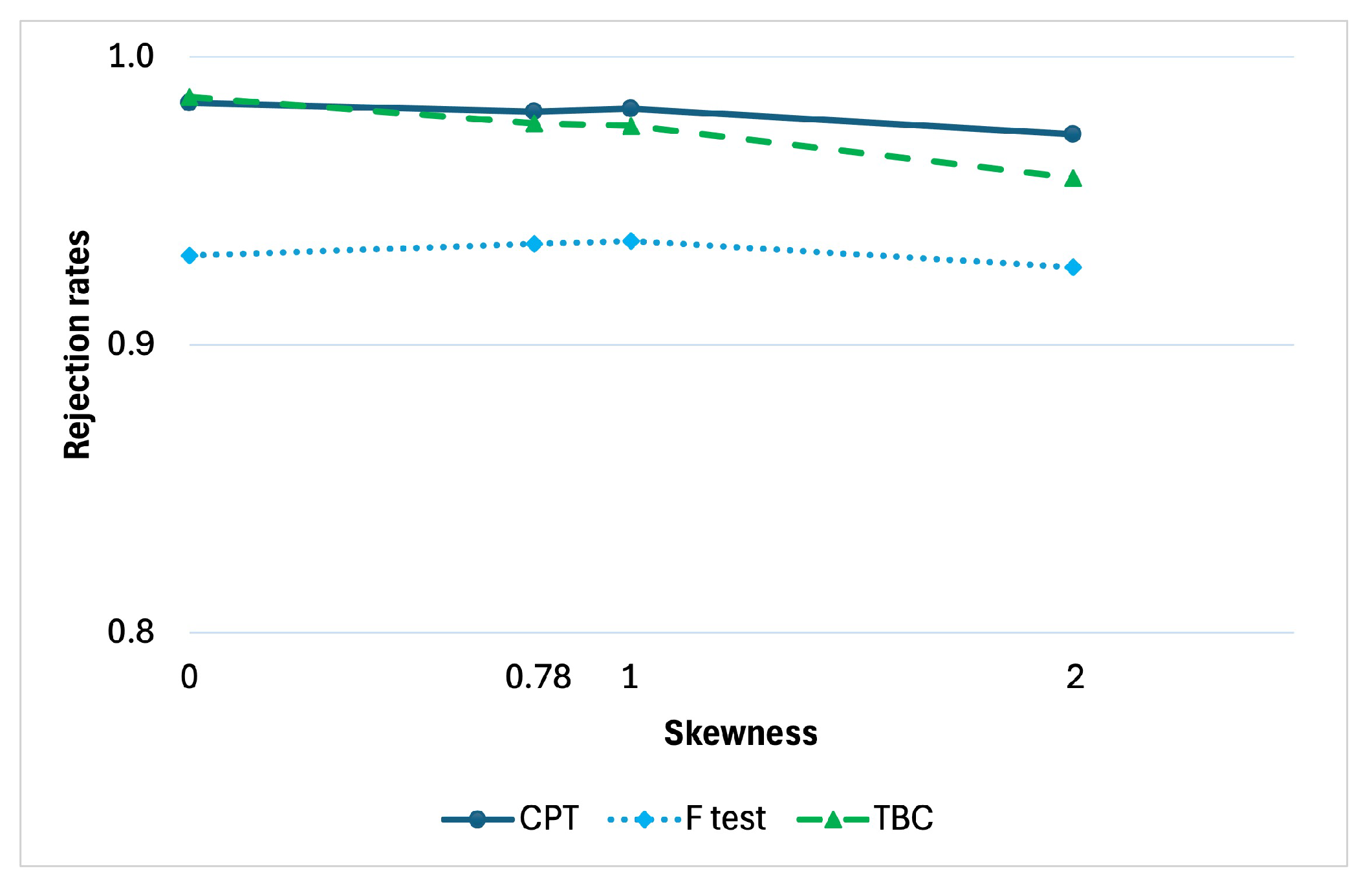
Furthermore, in Figure 3, the effect of skewness can be assessed when $n=100$. The rejection rates of the three tests are represented as a function of the asymmetry of the error term distribution. We remind that the skewness is null when the errors are simulated under normality, and corresponds to $\sqrt{{\displaystyle \frac{8}{\mathrm{df}}}}$ when the assumed error distribution is chi-square with $df$ degrees of freedom. We considered four scenarios, by simulating under normality and under ${\chi }_{13}^2$, ${\chi }_8^2$, and ${\chi }_2^2$, corresponding to the skewness values 0, $0.78$, 1 and 2, respectively. Again, the CPT method seems to be more powerful regardless of the departure of the distribution skewness from the symmetric case typical of normality.

5. Application to Real Data

As said, the application example concerns the study of the effect of age and smoking habit on the medical insurance cost in the USA. Data relate to a small random sample of the American population selected for a survey on the topic. We observed from [46] that attributes such as being a smoker, BMI, and age are the most important factors in determining medical insurance costs. However, since BMI in our dataset exhibits limited variability, resulting in a generally homogeneous patient population in this regard, we decided not to include it among the factors and instead considered only smoking status and age. The data source is Kaggle (https://www.kaggle.com/datasets/mirichoi0218/insurance, accessed on 20 December 2024).

The regression model under consideration for such a case study is the following:

$$Y_i={\beta }_0+{\beta }_1·{\mathit{smoker}}_i+{\beta }_2·{\mathit{age}}_i+{\beta }_{12}·{\mathit{interaction}}_i+{\epsilon }_i$$

(7)

where $y_i$ is the charge of medical insurance costs for the i-th person, ${\mathrm{smoker}}_i$ is the dummy variable that takes the value 1 if the i-th person is a smoker and 0 otherwise, ${\mathrm{age}}_i$ is a dummy variable that takes the value 1 if the i-th person is at least 50 years old and 0 otherwise, and ${\mathrm{interaction}}_i$ is the product between ${\mathrm{smoker}}_i$ and ${\mathrm{age}}_i$, hence it takes the value 1 if both the dummy variables take the value 1, in other words, if the level of both factors changes with respect to the baseline (from no-smoker under 50 y.o. to smoker over 50 y.o.).

In the literature, the concept that the allocation of health care expenses is significantly influenced by age is widespread, a trend that becomes increasingly important as the baby boom generation grows older. After the first year, health-care costs are at their lowest for children, gradually rise throughout adulthood, and surge dramatically after the age of 50 [47]. It was proved that the annual costs for older adults are roughly four to five times higher than those for individuals in their early teenage years [48]. For this reason, we took 50 years as a threshold to define age as a dummy variable [49]. The considered sample was obtained with a random selection from the American adult population, composed of 1338 people. This random selection implies that the exchangeability of statistical units under the null hypothesis holds.

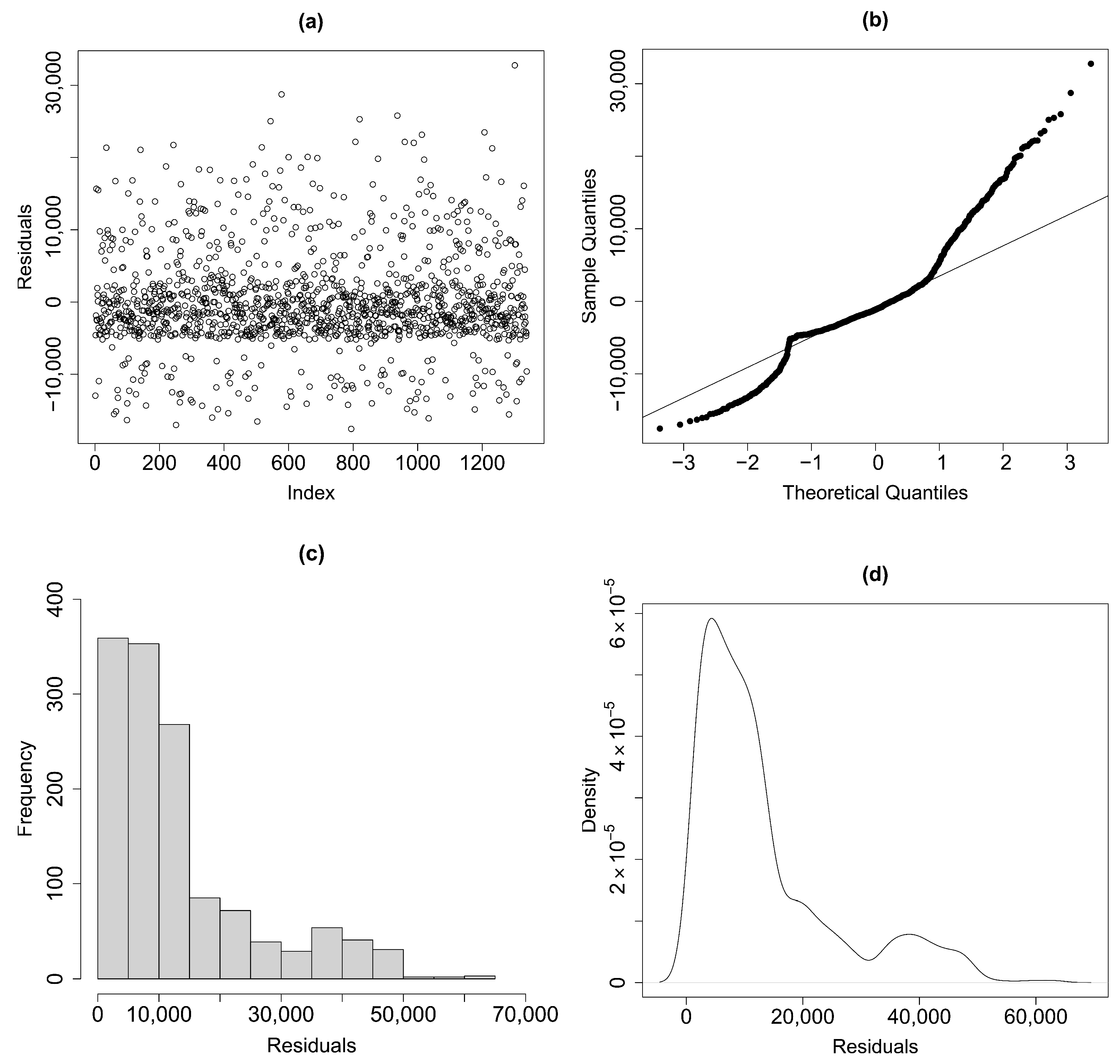
Figure 4 shows the scatter diagram, the normal Q–Q plot, the histogram and the density plot of the residuals. According to such plots, the assumptions of uncorrelated, homoskedastic, zero-mean errors seem to be plausible, but the distributions of the errors could be asymmetric. In particular, by examining the histogram and the density plot of the residuals, it can be observed that the distribution appears asymmetric, suggesting that the data are skewed to the left. This violates one of the typical assumptions of classic linear regression according to which errors follow a normal distribution. On the other hand, the same conclusion can be drawn from the normal Q–Q plot of residuals. In fact, the dots deviate from the straight line, indicating that the data may not follow the assumed theoretical distribution and therefore violate the normality assumption of the residuals. As a result, the assumption of normality for the model errors appears to be unmet and the use of the CPT test is preferable [50]. Indeed, as previously mentioned, the CPT method allows for the relaxation of the normality assumption, and there is no requirement to assume a specific family of probability distributions for the model error terms.

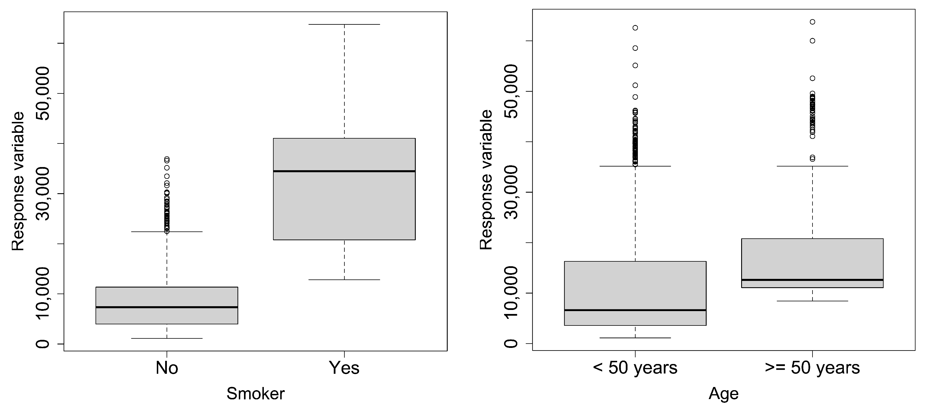
The boxplots of the response versus age and of the response versus being a smoker are reported in Figure 5. Such plots confirm the previous statements concerning the distribution asymmetry.

In Figure 6, the main effect plots and the interaction plot are represented. From a descriptive point of view, a variation in the means in both the main effect plots is shown, which is much more evident in the case of being a smoker. Conversely, in the interaction plot, the two segments tends to be parallel so there may not be an interaction between the two factors.

The goal of the analysis is to test the system of hypotheses defined in Section 3. To this aim, the non-parametric test presented was applied to such data. The significance level was set to $0.05$. The overall p-value of the CPT is equal to $0.0002$. This is less than the significance level $\alpha =0.05$ which leads to the rejection of the null hypothesis of no effect. The partial p-values related to the tests on the significance of the coefficient estimates adjusted with the Bonferroni–Holm correction are shown in

Table 1. Estimation of the coefficients, partial p-values on the significance of the coefficients estimates adjusted with the Bonferroni–Holm method (significance in bold).

	Estimate	Adjusted p-Values
Intercept	6313.9
Smoker	23,525.3	0.0003
Age	7117.0	0.0003
Interaction	1792.1	0.3464

. According to such adjusted p-values, the significance of the overall test can be attributed to the regression coefficients related to being a smoker and age but not to the interaction. Since the estimates of the regression coefficients are positive in both cases, we can state that being a smoker and being at least 50 years old positively influence medical insurance costs.

6. Concluding Remarks

This work is inspired by the study of the effects of age and smoking status on the insurance cost for the population in the USA. The main scientific contribution of the work consists of the application of an innovative non-parametric method, based on the CPT approach, to jointly test the main effects of the two binary factors and their interaction effect. The proposed method involves using permutation tests to assess the significance of individual coefficients, and combining the p-values of such partial tests to address the two-way ANOVA problem. The good power performance of the CPT compared to the F-test was shown in the Monte Carlo simulation study. The test was proved to be powerful, unbiased and consistent, regardless of the skewness of the error distribution.

The application of the proposed method to the interesting case study of medical insurance costs led to empirical evidence in favor of the hypothesis that age and being a smoker, each has a positive effect, whilst there is not an interaction effect. The findings of this research will practically support policymakers, insurance providers, and potential medical insurance buyers in making conscious decisions about choosing policies that meet their specific needs. A future extension of this work could explore the method’s performance on datasets with more complex dependence structures or alternative parametric models.

Possible future developments related to this work may involve the implementation of parallel computing techniques. These techniques serve as valuable tools for accelerating a wide range of algorithms, including Monte Carlo simulations. Indeed, the use of parallel computing can significantly enhance the efficiency of Monte Carlo simulations. Furthermore, the proposed method could be expanded in future work to cases of ANOVA with higher-order interactions or multi-level factors. For instance, in a three-way ANOVA (i.e., with three factors), it would be necessary to examine three main effects, three two-way interactions, and one three-way interaction.