Linear Sixth-Order Conservation Difference Scheme for KdV Equation

Abstract

A numerical investigation is conducted for the initial boundary value problem of the Korteweg–de Vries (KdV) equation with homogeneous boundary conditions. Using the average implicit difference discretization, a second-order theoretical accuracy in time is achieved. For the spatial direction, a center-symmetric discretization coupled with the extrapolation technique is employed, yielding a three-level linear difference method with sixth-order accuracy. Consequently, the integration of these methods results in a linear finite difference scheme that accurately simulates the two conserved quantities of the original problem. Furthermore, theoretical results, including the convergence and stability of the proposed scheme, are proved using the discrete Sobolev inequality and the discrete Gronwall inequality. Numerical experiments validate the reliability of the scheme.

1. Introduction

Korteweg and de Vries established a partial differential equation related to unidirectional shallow water waves for studying small amplitude long wave motion, given by

$$u_t+\alpha u{u}_x+u_{xxx}=0,$$

(1)

namely the Korteweg–de Vries (KdV) equation [1], where $\alpha$ is a non-zero real constant. After Gardner et al. [2] and Morikawa et al. [3] re-derived the KdV equation when analyzing collisionless water magnetic waves, an increasing number of scholars have discovered numerous applications of the KdV equation in engineering, physics, and other sciences, such as plasma physics, particle physics, and fluid mechanics. During the same time, research on the relevant properties and analytical solutions of the KdV equation has also progressed. For instance, Miura et al. [4] discovered conservation laws and motion constants of the KdV Equation (1) through nonlinear transformations. Su et al. [5] proved that many nonlinear evolution equations can be simplified into the KdV equation.

In pursuit of analytical solutions to the KdV Equation (1), various methods have been successively proposed, including the direct scattering transform method [6], the Lie group method [7], and the direct algebraic method [8]. However, the analytical solutions obtained through these methods are typically limited to specific forms. Consequently, research on numerical methods for the KdV Equation (1), such as the finite element method [9,10,11], the finite volume method [12], the meshless method based on radial basis functions [13] and the finite difference method [14,15,16,17,18,19], also has a significant practical value.

Among the numerous numerical methods, the finite difference method is particularly favored due to its simplicity in construction and ease of programming implementation. Zabusky et al. [14] were the first to propose an explicit finite difference scheme to obtain the numerical solution of the KdV equation. They observed that a series of soliton waves satisfying the KdV Equation (1) maintained their wave shape and velocity after colliding with each other, which are known as soliton collisions. Wang et al. [15] considered the scenario where the nonlinear term of the KdV equation dominates over the dispersion term. Based on explicit or implicit schemes, they conducted numerical studies and concluded that the numerical solution of the equation exhibits good stability when the nonlinear term is dominant. Building upon the work in [14], Vliegenthart et al. [16] further considered the KdV equation with a dissipative term and developed corresponding explicit difference schemes for both cases with and without dissipation. Eventually, numerical experiments verified that both schemes are conditionally stable. Greig et al. [17] proposed an implicit finite difference scheme and analyzed its stability and dispersion properties. Compared to the Zabusky–Kruskal method [14], this method reduced the computational space required and has become one of the most significant methods for numerical solutions of the KdV equation. For additional results on various difference schemes, please refer to references [18,19].

In recent years, there has increasing scholarly attention toward high-accuracy methods for solving the KdV equation. Previous research efforts, particularly those documented in [20,21], have made significant contributions through the development of an implicit compact finite difference scheme and a nonlinear difference scheme, respectively. These schemes achieve sixth-order spatial accuracy through the implementation of orthogonal decomposition and extrapolation techniques. However, the investigation in [20] is limited to numerical verification without providing theoretical analysis or numerical analysis of the conservation laws associated with the KdV Equation (1). Furthermore, the nonlinear iterative nature of the scheme proposed in [21] results in considerable computational overhead, potentially limiting its practical application.

Consider the following initial and boundary value problems of the KdV equation:

$$\begin{array}{ccc}& & u_t+\alpha u{u}_x+u_{xx}=0,(x,t)\in (x_L,x_R)\times (0,T],\hfill \end{array}$$

(2)

$$\begin{array}{ccc}& & u(x,0)=u_0\left(x\right),x\in [x_L,x_R],\hfill \end{array}$$

(3)

$$\begin{array}{ccc}& & u(x_L,t)=u(x_R,t)=0,u_x(x_R,t)=0,t\in [0,T],\hfill \end{array}$$

(4)

where $u_0\left(x\right)$ is a known function.

The single solitary wave solution of the KdV Equation (1) is

$$u(x,t)={\displaystyle \frac{12k^2}{\alpha }}sec{h}^2(kx-4k^{3}t),$$

where k is an arbitrary constant. Therefore, the physical boundary condition of the KdV Equation (1) satisfies

$$\begin{array}{c}\hfill u(x,t)\to 0,(t>0),\mathrm{as}\left|x\right|\to \infty .\end{array}$$

If $-x_L\gg 0$ and $x_R\gg 0$, the initial boundary value problem (2)–(4) is consistent with the Cauchy problem associated with the KdV Equation (1). This initial boundary value problem possesses two conservative quantities [4,21]:

$$\begin{array}{ccc}& & Q\left(t\right)={\int }_{x_L}^{x_R}u(x,t)dx={\int }_{x_L}^{x_R}{u}_0(x,t)dx=Q\left(0\right),\hfill \end{array}$$

(5)

$$\begin{array}{ccc}& & E\left(t\right)={\parallel u\parallel }_{L_2}^2={\parallel u_0\parallel }_{L_2}^2=E\left(0\right),\hfill \end{array}$$

(6)

where $Q\left(0\right)$ and $E\left(0\right)$ are constants that are only related to the initial condition.

In this paper, an average implicit difference scheme is employed in the temporal direction to attain second-order theoretical accuracy. Subsequently, a difference discretization technique, combined with extrapolation technology, is used in the spatial direction to achieve sixth-order theoretical accuracy. Consequently, a three-level linear difference scheme with sixth-order spatial accuracy is constructed for the initial boundary value problem (2)–(4). The conservative quantities of (5) and (6) could be accurately simulated. In addition, a comprehensive theoretical analysis is provided, which addresses convergence, stability, and other properties. Finally, numerical verifications are presented.

The remaining part of this paper is organized as follows. In Section 2, a numerical scheme and conservative laws are given. In Section 3, existence and uniqueness of the numerical solutions are presented. In Section 4, the convergence and stability of the scheme are analyzed. In Section 5, some numerical results are provided to test the theoretical results and computational efficiency of the proposed scheme.

2. Finite Difference Scheme and Conservation Laws

For the domain $[x_L,x_R]\times [0,T]$, set $h=(x_R-x_L)/J$ as the step size for the spatial grid, and set $\tau$ as the step size for the temporal direction such that $x_j=x_L+jh(0\le j\le J)$, $t_n=n\tau$ $(n=0,1,2,\cdots ,N,N=[T/\tau \left]\right)$. Denote $u_j^n=u(x_j,t_n)$ as the exact value of $u(x,t)$ and denote $U_j^n\approx u(x_j,t_n)$ as the approximation of $u(x,t)$ at point $(x_j,t_n)$, respectively. Consequently, $e_j^n=u_j^n-U_j^n$ is the error between $u_j^n$ and $U_j^n$. In the following, C denotes a general positive constant, which may have different values in different occurrences. Define the following:

$$\begin{array}{ccc}& & {\left(U_j^n\right)}_t={\displaystyle \frac{U_j^{n+1}-U_j^n}{\tau }},{\left(U_j^n\right)}_x={\displaystyle \frac{U_{j+1}^n-U_j^n}{h}},{\left(U_j^n\right)}_{\overline{x}}={\displaystyle \frac{U_j^n-U_{j-1}^n}{h}},\hfill \\ & & {\left(U_j^n\right)}_{\widehat{x}}={\displaystyle \frac{U_{j+1}^n-U_{j-1}^n}{2h}},{\left(U_j^n\right)}_{\ddot{x}}={\displaystyle \frac{U_{j+2}^n-U_{j-2}^n}{4h}},{\left(U_j^n\right)}_{\tilde{x}}={\displaystyle \frac{U_{j+3}^n-U_{j-3}^n}{6h}},\hfill \\ & & {\overline{U}}_j^n={\displaystyle \frac{U_j^{n+1}+U_j^{n-1}}{2}},U_j^{n+{\displaystyle \frac{1}{2}}}={\displaystyle \frac{U_j^{n+1}+U_j^n}{2}},U_j^{n-{\displaystyle \frac{1}{2}}}={\displaystyle \frac{U_j^n+U_j^{n-1}}{2}},\hfill \\ & & \langle U^n,V^n\rangle =h\sum _{j=1}^{J-1}{U}_j^n{V}_j^n,\parallel U^n{\parallel }^2=\langle U^n,U^n\rangle ,\parallel U^n{\parallel }_{\infty }=\underset{1\le j\le J-1}{max}\parallel U_j^n\parallel ,\hfill \\ & & Z_h^0=\{U=\left(U_j\right)|U_{0-i}=U_{J+i}=0,i=0,1,2,3;j=-3,-2,\cdots ,J+2,J+3\}.\hfill \end{array}$$

Based on these definitions, we can present the following lemma for the theoretical analysis in the next section.

Lemma 1

(Summation by Parts Formula [21,22]). For any mesh functions $U=\left\{U_j\right|j=0,1,2,...,J\}$ and $V=\left\{V_j\right|j=0,1,2,...,J\}$, we have

$$\begin{array}{c}\hfill h\sum _{j=0}^{J-1}{\left(V_j\right)}_x{U}_j=-h\sum _{j=1}^J{V}_j{\left(U_j\right)}_{\overline{x}}+V_J{U}_J-V_0{U}_0\end{array}$$

and

$$\begin{array}{c}\hfill h\sum _{j=1}^{J-1}\left(U_j\right){\left(V_j\right)}_{x\overline{x}}=-h\sum _{j=0}^{J-1}{\left(U_j\right)}_x{\left(U_j\right)}_x+U_J{\left(V_J\right)}_{\overline{x}}-U_0{\left(V_0\right)}_x.\end{array}$$

According to Lemma 1, if $U,V\in Z_h^0$, the following results hold:

$$\begin{array}{ccc}& & \langle U_x,V\rangle =-\langle U,V_{\overline{x}}\rangle ,\langle U_{x\overline{x}},V\rangle =-\langle U_x,V_x\rangle ,\langle U_{\widehat{x}},V\rangle =-\langle U,V_{\widehat{x}}\rangle ,\hfill \\ & & \langle U_{\ddot{x}},V\rangle =-\langle U,V_{\ddot{x}}\rangle ,\langle U_{\tilde{x}},V\rangle =-\langle U,V_{\tilde{x}}\rangle ,\hfill \end{array}$$

For the problem (2)–(4), the corresponding linear finite difference scheme is constructed as follows:

$$\begin{array}{ccc}& & {\left(U_j^n\right)}_{\widehat{t}}+\alpha \phi (U_j^n,{\overline{U}}_j^n)+\varphi \left({\overline{U}}_j^n\right)=0,j=1,2,\cdots ,J-1;n=2,3,\cdots ,N-1,\hfill \end{array}$$

(7)

$$\begin{array}{ccc}& & U_j^0=u_0\left(x_j\right),j=0,1,2,\cdots ,J,\hfill \end{array}$$

(8)

$$\begin{array}{ccc}& & U^n\in Z_h^0,n=0,1,2,\cdots ,N,\hfill \end{array}$$

(9)

where

$$\begin{array}{ccc}& & \phi (U_j^n,{\overline{U}}_j^n)={\phi }_1(U_j^n,{\overline{U}}_j^n)+{\phi }_2(U_j^n,{\overline{U}}_j^n)+{\phi }_3(U_j^n,{\overline{U}}_j^n),\hfill \\ & & {\phi }_1(U_j^n,{\overline{U}}_j^n)={\displaystyle \frac{1}{2}}[U_j^n{\left({\overline{U}}_j^n\right)}_{\widehat{x}}+{\left(U_j^n{\overline{U}}_j^n\right)}_{\widehat{x}}],\hfill \\ & & {\phi }_2(U_j^n,{\overline{U}}_j^n)=-{\displaystyle \frac{1}{5}}[U_j^n{\left({\overline{U}}_j^n\right)}_{\ddot{x}}+{\left(U_j^n{\overline{U}}_j^n\right)}_{\ddot{x}}],\hfill \\ & & {\phi }_3(U_j^n,{\overline{U}}_j^n)={\displaystyle \frac{1}{30}}[U_j^n{\left({\overline{U}}_j^n\right)}_{\tilde{x}}+{\left(U_j^n{\overline{U}}_j^n\right)}_{\tilde{x}}],\hfill \\ & & \varphi \left({\overline{U}}_j^n\right)={\displaystyle \frac{26}{15}}{\left({\overline{U}}_j^n\right)}_{x\overline{x}\widehat{x}}-{\displaystyle \frac{6}{5}}{\left({\overline{U}}_j^n\right)}_{x\overline{x}\ddot{x}}+{\displaystyle \frac{7}{15}}{\left({\overline{U}}_j^n\right)}_{\widehat{x}\widehat{x}\ddot{x}}.\hfill \end{array}$$

Now that the difference scheme (7)–(9) does not start automatically, it is necessary to first select a two-level difference scheme with a theoretical accuracy of $O({\tau }^2+h^6)$ [21] for initialization.

From the difference scheme (7)–(9), the following conclusion can be drawn from the numerical simulation of conservation laws (5) and (6):

Theorem 1.

The difference scheme (7)–(9) has the following conservative quantities:

$$\begin{array}{ccc}& & Q^n={\displaystyle \frac{h}{2}}\sum _{j=1}^{J-1}(U_j^{n+1}+U_j^n)+{\displaystyle \frac{\alpha }{4}}h\tau \sum _{j=1}^{J-1}{U}_j^n{\left(U_j^{n+1}\right)}_{\widehat{x}}-{\displaystyle \frac{\alpha }{10}}h\tau \sum _{j=1}^{J-1}{U}_j^n{\left(U_j^{n+1}\right)}_{\ddot{x}}\hfill \end{array}$$

$$\begin{array}{ccc}& & +{\displaystyle \frac{\alpha }{60}}h\tau \sum _{j=1}^{J-1}{U}_j^n{\left(U_j^{n+1}\right)}_{\tilde{x}}=Q^{n-1}=\cdots =Q^0,\hfill \end{array}$$

(10)

$$\begin{array}{ccc}& & E^n={\displaystyle \frac{1}{2}}(\parallel U^{n+1}{\parallel }^2+\parallel U^n{\parallel }^2)=E^{n-1}=\cdots =E^0,\hfill \end{array}$$

(11)

for $n=1,2,\cdots ,N-1$.

Proof of Theorem 1.

By summing Equation (7) for j from 1 to $J-1$ and multiplying both sides by h, we obtain

$$\begin{array}{c}\hfill h\sum _{j=1}^{J-1}{\displaystyle \frac{U_j^{n+1}-U_j^{n-1}}{2\tau }}+\alpha h\sum _{j=1}^{J-1}\phi (U_j^n,{\overline{U}}_j^n)+h\sum _{j=1}^{J-1}\varphi \left({\overline{U}}_j^n\right)=0.\end{array}$$

(12)

Combining the boundary condition (9) and the summation by parts [23], we have

$$\begin{array}{ccc}& & h\sum _{j=1}^{J-1}{U}_j^n{\left({\overline{U}}_j^n\right)}_{\widehat{x}}={\displaystyle \frac{1}{2}}h\sum _{j=1}^{J-1}{U}_j^n{(U_j^{n+1}+U_j^{n-1})}_{\widehat{x}}\hfill \\ & & ={\displaystyle \frac{1}{2}}h\sum _{j=1}^{J-1}{U}_j^n{\left(U_j^{n+1}\right)}_{\widehat{x}}+{\displaystyle \frac{1}{2}}h\sum _{j=1}^{J-1}{U}_j^n{\left(U_j^{n-1}\right)}_{\widehat{x}}\hfill \\ & & ={\displaystyle \frac{1}{2}}h\sum _{j=1}^{J-1}{U}_j^n{\left(U_j^{n+1}\right)}_{\widehat{x}}-{\displaystyle \frac{1}{2}}h\sum _{j=1}^{J-1}{U}_j^{n-1}{\left(U_j^n\right)}_{\widehat{x}}.\hfill \end{array}$$

(13)

Similarly,

$$\begin{array}{c}\hfill h\sum _{j=1}^{J-1}{U}_j^n{\left({\overline{U}}_j^n\right)}_{\ddot{x}}={\displaystyle \frac{1}{2}}h\sum _{j=1}^{J-1}{U}_j^n{\left(U_j^{n+1}\right)}_{\ddot{x}}-{\displaystyle \frac{1}{2}}h\sum _{j=1}^{J-1}{U}_j^{n-1}{\left(U_j^n\right)}_{\ddot{x}},\end{array}$$

(14)

$$\begin{array}{c}\hfill h\sum _{j=1}^{J-1}{U}_j^n{\left({\overline{U}}_j^n\right)}_{\tilde{x}}={\displaystyle \frac{1}{2}}h\sum _{j=1}^{J-1}{U}_j^n{\left(U_j^{n+1}\right)}_{\tilde{x}}-{\displaystyle \frac{1}{2}}h\sum _{j=1}^{J-1}{U}_j^{n-1}{\left(U_j^n\right)}_{\tilde{x}}.\end{array}$$

(15)

According to

$$\begin{array}{c}\hfill h\sum _{j=1}^{J-1}{\left(U_j^n{\overline{U}}_j^n\right)}_{\widehat{x}}=0,h\sum _{j=1}^{J-1}{\left(U_j^n{\overline{U}}_j^n\right)}_{\ddot{x}}=0,h\sum _{j=1}^{J-1}{\left(U_j^n{\overline{U}}_j^n\right)}_{\tilde{x}}=0,\end{array}$$

(16)

it follows from (13)–(16) that

$$\begin{array}{ccc}& & h\sum _{j=1}^{J-1}\phi (U_j^n,{\overline{U}}_j^n)={\displaystyle \frac{1}{4}}h\sum _{j=1}^{J-1}{U}_j^n{\left(U_j^{n+1}\right)}_{\widehat{x}}-{\displaystyle \frac{1}{4}}h\sum _{j=1}^{J-1}{U}_j^{n-1}{\left(U_j^n\right)}_{\widehat{x}}-{\displaystyle \frac{1}{10}}h\sum _{j=1}^{J-1}{U}_j^n{\left(U_j^{n+1}\right)}_{\ddot{x}}\hfill \\ & & +{\displaystyle \frac{1}{10}}h\sum _{j=1}^{J-1}{U}_j^{n-1}{\left(U_j^n\right)}_{\ddot{x}}+{\displaystyle \frac{1}{60}}h\sum _{j=1}^{J-1}{U}_j^n{\left(U_j^{n+1}\right)}_{\tilde{x}}-{\displaystyle \frac{1}{60}}h\sum _{j=1}^{J-1}{U}_j^{n-1}{\left(U_j^n\right)}_{\tilde{x}}.\hfill \end{array}$$

(17)

Since

$$\begin{array}{c}\hfill h\sum _{j=1}^{J-1}{\left({\overline{U}}_j^n\right)}_{x\overline{x}\widehat{x}}=0,h\sum _{j=1}^{J-1}{\left({\overline{U}}_j^n\right)}_{x\overline{x}\ddot{x}}=0,h\sum _{j=1}^{J-1}{\left({\overline{U}}_j^n\right)}_{\widehat{x}\widehat{x}\ddot{x}}=0,\end{array}$$

that is,

$$\begin{array}{c}\hfill h\sum _{j=1}^{J-1}\varphi ({\overline{U}}_j^n)=0.\end{array}$$

(18)

By substituting (17) and (18) into (12), by the definition of $Q^n$, we obtain the result (10).

Taking the inner product of (7) with $2{\overline{U}}^n$, one can obtain

$$\begin{array}{c}\hfill \parallel U^n{\parallel }_{\widehat{t}}^2+2\alpha \langle \phi (U^n,{\overline{U}}^n),{\overline{U}}^n\rangle +2\langle \varphi \left({\overline{U}}^n\right),{\overline{U}}^n\rangle =0.\end{array}$$

(19)

From the boundary condition (9) and the summation by parts [23], the following result also holds:

$$\begin{array}{ccc}& & \langle {\phi }_1(U^n,{\overline{U}}^n),{\overline{U}}^n\rangle ={\displaystyle \frac{1}{2}}h\sum _{j=1}^{J-1}[U_j^n{\left({\overline{U}}_j^n\right)}_{\widehat{x}}+{\left(U_j^n{\overline{U}}_j^n\right)}_{\widehat{x}}]{\overline{U}}_j^n\hfill \\ & & ={\displaystyle \frac{1}{2}}h\sum _{j=1}^{J-1}{U}_j^n{\overline{U}}_j^n{\left({\overline{U}}_j^n\right)}_{\widehat{x}}+{\displaystyle \frac{1}{2}}h\sum _{j=1}^{J-1}{\left(U_j^n{\overline{U}}_j^n\right)}_{\widehat{x}}{\overline{U}}_j^n\hfill \\ & & ={\displaystyle \frac{1}{2}}h\sum _{j=1}^{J-1}{U}_j^n{\overline{U}}_j^n{\left({\overline{U}}_j^n\right)}_{\widehat{x}}-{\displaystyle \frac{1}{2}}h\sum _{j=1}^{J-1}{U}_j^n{\overline{U}}_j^n{\left({\overline{U}}_j^n\right)}_{\widehat{x}}=0.\hfill \end{array}$$

Notice that

$$\begin{array}{c}\hfill \langle {\phi }_2(U^n,{\overline{U}}^n),{\overline{U}}^n\rangle =0,\langle {\phi }_3(U^n,{\overline{U}}^n),{\overline{U}}^n\rangle =0,\end{array}$$

Specifically,

$$\begin{array}{c}\hfill \langle \phi (U^n,{\overline{U}}^n),{\overline{U}}^n\rangle =0.\end{array}$$

(20)

On the other hand, if follows from Lemma 1 that

$$\begin{array}{c}\hfill \langle {\overline{U}}_{x\overline{x}\widehat{x}}^n,{\overline{U}}^n\rangle =-\langle {\overline{U}}_{x\widehat{x}}^n,{\overline{U}}_x^n\rangle =-\langle {\left({\overline{U}}_x^n\right)}_{\widehat{x}},{\overline{U}}_x^n\rangle =\langle \left({\overline{U}}_x^n\right),{\left({\overline{U}}_x^n\right)}_{\widehat{x}}\rangle =0.\end{array}$$

Obviously, $\langle {\overline{U}}_{x\overline{x}\widehat{x}}^n,{\overline{U}}^n\rangle =0$. Similarly, $\langle {\overline{U}}_{x\overline{x}\ddot{x}}^n,{\overline{U}}^n\rangle =0$, $\langle {\overline{U}}_{\widehat{x}\widehat{x}\ddot{x}}^n,{\overline{U}}^n\rangle =0$. Therefore, we obtain

$$\begin{array}{c}\hfill \langle \varphi \left({\overline{U}}^n\right),{\overline{U}}^n\rangle =\langle {\displaystyle \frac{26}{15}}{\left({\overline{U}}_j^n\right)}_{x\overline{x}\widehat{x}}-{\displaystyle \frac{6}{5}}{\left({\overline{U}}_j^n\right)}_{x\overline{x}\ddot{x}}+{\displaystyle \frac{7}{15}}{\left({\overline{U}}_j^n\right)}_{\widehat{x}\widehat{x}\ddot{x}},{\overline{U}}^n\rangle =0.\end{array}$$

(21)

Finally, by substituting (20) and (21) into (19), we have

$$\begin{array}{c}\hfill \parallel U^n{\parallel }_{\widehat{t}}^2={\displaystyle \frac{\parallel U^{n+1}{\parallel }^2-{\parallel U^n\parallel }^2}{2\tau }}=0.\end{array}$$

By the definition of $E^n$, we can obtain (11). □

Remark 1.

The numerical scheme (7)–(9) is focused on the KdV equation with homogeneous boundary conditions, because it is consistent with the corresponding physical boundary conditions and has the property of energy conservation. According to Lemma 1, the proposed numerical scheme is equally effective for KdV equations with periodic boundary conditions. However, if non-homogeneous boundary conditions are considered, the numerical scheme no longer holds the property of energy conservation.

3. Existence and Uniqueness of the Difference Solution

Theorem 2.

There exists $U^{n+1}(0\le n\le N-1)$ that uniquely satisfies the difference scheme (7)–(9).

Proof of Theorem 2.

We employ mathematical induction to prove this result. According to the initial value (8), $U^0$ is unique. Then, we use the two-level difference scheme [21] to compute $U^1$, which means that $U^1$ is uniquely determined. Suppose that both $U^{n-1}$ and $U^n$ have unique solutions. From (7), $U^{n+1}$ satisfies

$$\begin{array}{c}\hfill {\displaystyle \frac{1}{2\tau }}{U}_j^{n+1}+{\displaystyle \frac{\alpha }{2}}\phi (U_j^n,U_j^{n+1})+{\displaystyle \frac{1}{2}}\varphi \left(U_j^{n+1}\right)=0,j=0,1,\cdots ,J.\end{array}$$

(22)

Taking the inner product of (22) with $U^{n+1}$ leads to

$$\begin{array}{c}\hfill {\displaystyle \frac{1}{2\tau }}{\parallel U^{n+1}\parallel }^2+{\displaystyle \frac{\alpha }{2}}\langle \phi (U^n,U^{n+1}),U^{n+1}\rangle +{\displaystyle \frac{1}{2}}\langle \varphi \left(U^{n+1}\right),U^{n+1}\rangle =0.\end{array}$$

Similar to (20) and (21), we obtain

$$\begin{array}{c}\hfill \langle \phi (U^n,U^{n+1}),U^{n+1}\rangle =0,\langle \varphi \left(U^{n+1}\right),U^{n+1}\rangle =0,\end{array}$$

which implies that $\parallel U^{n+1}{\parallel }^2=0$. Therefore, the homogeneous linear system (22) only has the zero solution. This completes the proof. □

4. Convergence and Stability

By the Taylor expansion, if $u\left(x\right)$ is smooth enough, we have

$$\begin{array}{ccc}& & {\left(u_j\right)}_{\widehat{x}}={\displaystyle \frac{\mathrm{d}u}{\mathrm{d}x}}{|}_{x=x_j}+{\displaystyle \frac{1}{3!}}{h}^2{\displaystyle \frac{{\mathrm{d}}^{3}u}{\mathrm{d}{x}^3}}{|}_{x=x_j}+{\displaystyle \frac{1}{5!}}{h}^4{\displaystyle \frac{{\mathrm{d}}^{5}u}{\mathrm{d}{x}^5}}{|}_{x=x_j}+O\left(h^6\right),\hfill \\ & & {\left(u_j\right)}_{\ddot{x}}={\displaystyle \frac{\mathrm{d}u}{\mathrm{d}x}}{|}_{x=x_j}+{\displaystyle \frac{4}{3!}}{h}^2{\displaystyle \frac{{\mathrm{d}}^{3}u}{\mathrm{d}{x}^3}}{|}_{x=x_j}+{\displaystyle \frac{16}{5!}}{h}^4{\displaystyle \frac{{\mathrm{d}}^{5}u}{\mathrm{d}{x}^5}}{|}_{x=x_j}+O\left(h^6\right),\hfill \\ & & {\left(u_j\right)}_{\tilde{x}}={\displaystyle \frac{\mathrm{d}u}{\mathrm{d}x}}{|}_{x=x_j}+{\displaystyle \frac{9}{3!}}{h}^2{\displaystyle \frac{{\mathrm{d}}^{3}u}{\mathrm{d}{x}^3}}{|}_{x=x_j}+{\displaystyle \frac{81}{5!}}{h}^4{\displaystyle \frac{{\mathrm{d}}^{5}u}{\mathrm{d}{x}^5}}{|}_{x=x_j}+O\left(h^6\right),\hfill \\ & & {\left(u_j\right)}_{x\overline{x}\widehat{x}}={\displaystyle \frac{{\mathrm{d}}^{3}u}{\mathrm{d}{x}^3}}{|}_{x=x_j}+{\displaystyle \frac{1}{4}}{h}^2{\displaystyle \frac{{\mathrm{d}}^{5}u}{\mathrm{d}{x}^5}}{|}_{x=x_j}+{\displaystyle \frac{1}{40}}{h}^4{\displaystyle \frac{{\mathrm{d}}^{7}u}{\mathrm{d}{x}^7}}{|}_{x=x_j}+O\left(h^6\right),\hfill \\ & & {\left(u_j\right)}_{x\overline{x}\ddot{x}}={\displaystyle \frac{{\mathrm{d}}^{3}u}{\mathrm{d}{x}^3}}{|}_{x=x_j}+{\displaystyle \frac{3}{4}}{h}^2{\displaystyle \frac{{\mathrm{d}}^{5}u}{\mathrm{d}{x}^5}}{|}_{x=x_j}+{\displaystyle \frac{23}{120}}{h}^4{\displaystyle \frac{{\mathrm{d}}^{7}u}{\mathrm{d}{x}^7}}{|}_{x=x_j}+O\left(h^6\right),\hfill \\ & & {\left(u_j\right)}_{\widehat{x}\widehat{x}\ddot{x}}={\displaystyle \frac{{\mathrm{d}}^{3}u}{\mathrm{d}{x}^3}}{|}_{x=x_j}+h^2{\displaystyle \frac{{\mathrm{d}}^{5}u}{\mathrm{d}{x}^5}}{|}_{x=x_j}+{\displaystyle \frac{2}{5}}{h}^4{\displaystyle \frac{{\mathrm{d}}^{7}u}{\mathrm{d}{x}^7}}{|}_{x=x_j}+O\left(h^6\right),\hfill \end{array}$$

for $h\to 0$.

To obtain the sixth-order accuracy in space, we can use extrapolation combination techniques of ${\left(u_j\right)}_{\widehat{x}},{\left(u_j\right)}_{\ddot{x}}$ and ${\left(u_j\right)}_{\tilde{x}}$ to approximate the discretization of the term ${\displaystyle \frac{du}{dx}}{|}_{x=x_j}$. Suppose that there exist $a_1,a_2$ and $a_3$ such that

$$\begin{array}{c}\hfill a_1{\left(u_j\right)}_{\widehat{x}}+a_2{\left(u_j\right)}_{\ddot{x}}+a_3{\left(u_j\right)}_{\tilde{x}}={\displaystyle \frac{du}{dx}}{|}_{x=x_j}+O\left(h^6\right)\end{array}$$

and we can find the solutions $a_1={\displaystyle \frac{3}{2}}, a_2=-{\displaystyle \frac{3}{5}}$ and $a_3={\displaystyle \frac{1}{10}}$. Then,

$$\begin{array}{c}\hfill {\displaystyle \frac{3}{2}}{\left(u_j\right)}_{\widehat{x}}-{\displaystyle \frac{3}{5}}{\left(u_j\right)}_{\ddot{x}}+{\displaystyle \frac{1}{10}}{\left(u_j\right)}_{\tilde{x}}={\displaystyle \frac{\mathrm{d}u}{\mathrm{d}x}}{|}_{x=x_j}+O\left(h^6\right).\end{array}$$

(23)

By the same method, we also have

$$\begin{array}{c}\hfill {\displaystyle \frac{26}{15}}{\left(u_j\right)}_{x\overline{x}\widehat{x}}-{\displaystyle \frac{6}{5}}{\left(u_j\right)}_{x\overline{x}\ddot{x}}+{\displaystyle \frac{7}{15}}{\left(u_j\right)}_{\widehat{x}\widehat{x}\ddot{x}}={\displaystyle \frac{{\mathrm{d}}^{3}u}{\mathrm{d}{x}^3}}{|}_{x=x_j}+O\left(h^6\right).\end{array}$$

(24)

The truncation error of the difference scheme in [21] is set as

$$\begin{array}{ccc}& & r_j^n={\left(u_j^n\right)}_{\widehat{t}}+\alpha \phi (u_j^n,{\overline{u}}_j^n)+\varphi \left({\overline{u}}_j^n\right),j=1,2,\cdots ,J-1;n=1,2,\cdots ,N-1,\hfill \end{array}$$

(25)

$$\begin{array}{ccc}& & u_j^0=u_0\left(x_j\right),j=0,1,2,\cdots ,J,\hfill \end{array}$$

(26)

$$\begin{array}{ccc}& & u^n\in Z_h^0,n=0,1,2,\cdots ,N.\hfill \end{array}$$

(27)

By the difference discretization of problem (2)–(4) at point $(x_j,t_n)$, and the Taylor expansion, from (23) and (24), one can obtain

$$\begin{array}{c}\hfill |r_j^n|=O({\tau }^2+h^6).\end{array}$$

(28)

Moreover, since $u(x,t)$ has continuous third-order partial derivatives $u_{xxx}$ on a bounded closed domain $[x_L,x_R]\times [0,T]$, we have

$$\begin{array}{c}\hfill {\parallel u\parallel }_{L_{\infty }}\le C,{\parallel u_x\parallel }_{L_{\infty }}\le C.\end{array}$$

For the convenience of subsequent analysis, define the following constant:

$$\begin{array}{c}\hfill C_u=\underset{(x,t)\in [x_L,x_R]\times [0,T]}{max}\left\{\right|u(x,t)|,|u_x(x,t)|,|u_t(x,t)\left|\right\}.\end{array}$$

Lemma 2

([21]). For $\forall U\in Z_h^0$, we have

$$\begin{array}{c}\hfill \parallel U_{\widehat{x}}{\parallel }^2\le \parallel U_x{\parallel }^2,\parallel U_{\ddot{x}}{\parallel }^2\le \parallel U_{\widehat{x}}{\parallel }^2,\parallel U_{\tilde{x}}{\parallel }^2\le {\parallel U_{\widehat{x}}\parallel }^2.\end{array}$$

Lemma 3

([23,24]). Suppose that $\left\{w^n\right|n=0,1,2,\cdots ,N;N\tau \le T\}$ is non-negative mesh function, satisfying $w^n\le A+\tau {\sum }_{k=1}^n{B}_k{w}^k$, where A and $B_k(k=0,1,2,\cdots ,N)$ are non-negative constants, and then it holds

$$\begin{array}{c}\hfill \underset{1\le n\le N}{max}\left|w^n\right|\le A{e}^{\left(2\tau {\sum }_{l=1}^N{B}_l\right)}\end{array}$$

for a sufficiently small τ, in which τ satisfies $\tau ·\left({max}_{1\le k\le N}{B}_k\right)\le {\displaystyle \frac{1}{2}}$.

Theorem 3.

Suppose that $u_0\in H^2[x_L,x_R]$. If $\lambda ={\displaystyle \frac{11·\left|\alpha \right|·C_u}{15}}·{\displaystyle \frac{\tau }{h}}<1$, then the solution of scheme (7)–(9) converges to the solution of problem (2)–(4) with accuracy $O({\tau }^2+h^6)$.

Proof of Theorem 3.

Denote $e_j^n=u_j^n-U_j^n$. By subtracting (25)–(27) from (7)–(9), we obtain

$$\begin{array}{ccc}& & r_j^n={\left(e_j^n\right)}_{\widehat{t}}+\alpha \phi (u_j^n,{\overline{u}}_j^n)-\alpha \phi (U_j^n,{\overline{U}}_j^n)+\varphi \left({\overline{e}}_j^n\right),\hfill \end{array}$$

$$\begin{array}{ccc}& & j=1,2,\cdots ,J-1;n=1,2,\cdots ,N-1,\hfill \end{array}$$

(29)

$$\begin{array}{ccc}& & e_j^0=0,j=0,1,2,\cdots ,J,\hfill \end{array}$$

(30)

$$\begin{array}{ccc}& & e^n\in Z_h^0,n=0,1,2,\cdots ,N.\hfill \end{array}$$

(31)

Taking the inner product of (29) with $2{\overline{e}}^n$, we have

$$\begin{array}{c}\hfill \langle \phi (u^n,{\overline{e}}^n),{\overline{e}}^n\rangle =0,\langle \phi (e^n,{\overline{e}}^n),{\overline{e}}^n\rangle =0,\langle \varphi \left({\overline{e}}^n\right),2{\overline{e}}^n\rangle =0.\end{array}$$

Then, if follows from (20) that

$$\begin{array}{ccc}& & \langle r^n,2{\overline{e}}^n\rangle ={\parallel e^n\parallel }_{\widehat{t}}^2+2\alpha \langle \phi (u^n,{\overline{u}}^n)-\phi (U^n,{\overline{U}}^n),{\overline{e}}^n\rangle \hfill \\ & & =\parallel e^n{\parallel }_{\widehat{t}}^2+2\alpha \langle \phi (u^n,{\overline{u}}^n)-\phi (u^n-e^n,{\overline{u}}^n-{\overline{e}}^n),{\overline{e}}^n\rangle \hfill \\ & & =\parallel e^n{\parallel }_{\widehat{t}}^2+2\alpha \langle \phi (u^n,{\overline{e}}^n)+\phi (e^n,{\overline{u}}^n)-\phi (e^n,{\overline{e}}^n),{\overline{e}}^n\rangle \hfill \\ & & =\parallel e^n{\parallel }_{\widehat{t}}^2+2\alpha \langle \phi (e^n,{\overline{u}}^n),{\overline{e}}^n\rangle .\hfill \end{array}$$

(32)

By the boundary condition (31) and the summation by parts [23], one can obtain

$$\begin{array}{ccc}& & \langle {\phi }_1(e^n,{\overline{u}}^n),{\overline{e}}^n\rangle ={\displaystyle \frac{h}{2}}\sum _{j=1}^{J-1}{e}_j^n{\overline{e}}_j^n{\left({\overline{u}}_j^n\right)}_{\widehat{x}}-{\displaystyle \frac{h}{2}}\sum _{j=1}^{J-1}{e}_j^n{\overline{u}}_j^n{\left({\overline{e}}_j^n\right)}_{\widehat{x}}\hfill \\ & & ={\displaystyle \frac{h}{2}}\sum _{j=1}^{J-1}{e}_j^n{\overline{e}}_j^n{\left({\overline{u}}_j^n\right)}_{\widehat{x}}+{\displaystyle \frac{h}{2}}\sum _{j=1}^{J-1}{\left(e_j^n{\overline{u}}_j^n\right)}_{\widehat{x}}{\overline{e}}_j^n\hfill \\ & & ={\displaystyle \frac{h}{2}}\sum _{j=1}^{J-1}{e}_j^n{\overline{e}}_j^n{\left({\overline{u}}_j^n\right)}_{\widehat{x}}+{\displaystyle \frac{1}{4}}\sum _{j=1}^{J-1}(e_{j+1}^n{\overline{u}}_{j+1}^n-e_{j-1}^n{\overline{u}}_{j-1}^n){\overline{e}}_j^n\hfill \end{array}$$

$$\begin{array}{ccc}& & ={\displaystyle \frac{h}{2}}\sum _{j=1}^{J-1}{e}_j^n{\overline{e}}_j^n{\left({\overline{u}}_j^n\right)}_{\widehat{x}}+{\displaystyle \frac{1}{4}}\sum _{j=1}^{J-1}(e_{j+1}^n{\overline{e}}_j^n{\overline{u}}_{j+1}^n-e_{j+1}^n{\overline{e}}_j^n{\overline{u}}_j^n+e_{j+1}^n{\overline{e}}_j^n{\overline{u}}_j^n-e_j^n{\overline{e}}_{j+1}^n{\overline{u}}_j^{n}t)\hfill \\ & & ={\displaystyle \frac{h}{2}}\sum _{j=1}^{J-1}{e}_j^n{\overline{e}}_j^n{\left({\overline{u}}_j^n\right)}_{\widehat{x}}+{\displaystyle \frac{h}{4}}\sum _{j=1}^{J-1}{e}_{j+1}^n{\overline{e}}_j^n{\left({\overline{u}}_j^n\right)}_x\hfill \\ & & +{\displaystyle \frac{1}{8}}\sum _{j=1}^{J-1}{\overline{u}}_j^n[(e_j^{n+1}{e}_{j+1}^n-e_{j+1}^{n+1}{e}_j^n)-(e_j^n{e}_{j+1}^{n-1}-e_{j+1}^n{e}_j^{n-1})]\hfill \\ & & ={\displaystyle \frac{h}{2}}\sum _{j=1}^{J-1}{e}_j^n{\overline{e}}_j^n{\left({\overline{u}}_j^n\right)}_{\widehat{x}}+{\displaystyle \frac{h}{4}}\sum _{j=1}^{J-1}{e}_{j+1}^n{\overline{e}}_j^n{\left({\overline{u}}_j^{n}t\right)}_x+{\displaystyle \frac{1}{8}}[\sum _{j=1}^{J-1}{u}_j^{n+1/2}(e_j^{n+1}{e}_{j+1}^n-e_{j+1}^{n+1}{e}_j^n)\hfill \\ & & -\sum _{j=1}^{J-1}{u}_j^{n-1/2}(e_j^n{e}_{j+1}^{n-1}-e_{j+1}^n{e}_j^{n-1})]+{\displaystyle \frac{1}{16}}\sum _{j=1}^{J-1}(u_j^{n-1}-u_j^n)(e_j^{n+1}{e}_{j+1}^n-e_{j+1}^{n+1}{e}_j^n)\hfill \\ & & +{\displaystyle \frac{1}{16}}\sum _{j=1}^{J-1}(u_j^n-u_j^{n+1})(e_j^n{e}_{j+1}^{n-1}-e_{j+1}^n{e}_j^{n-1}).\hfill \end{array}$$

(33)

Similarly, the following results also hold:

$$\begin{array}{ccc}& & \langle {\phi }_2(e^n,{\overline{u}}^n),{\overline{e}}^n\rangle =-{\displaystyle \frac{h}{5}}\sum _{j=1}^{J-1}{e}_j^n{\overline{e}}_j^n{\left({\overline{u}}_j^n\right)}_{\ddot{x}}-{\displaystyle \frac{h}{10}}\sum _{j=1}^{J-1}{e}_{j+2}^n{\overline{e}}_j^n\left({\displaystyle \frac{{\overline{u}}_{j+2}^n-{\overline{u}}_j^n}{2h}}\right)\hfill \\ & & -{\displaystyle \frac{1}{20}}[\sum _{j=1}^{J-1}{u}_j^{n+{\displaystyle \frac{1}{2}}}(e_j^{n+1}{e}_{j+2}^n-e_{j+2}^{n+1}{e}_j^n)-\sum _{j=1}^{J-1}{u}_j^{n-{\displaystyle \frac{1}{2}}}(e_j^n{e}_{j+2}^{n-1}-e_{j+2}^n{e}_j^{n-1})]\hfill \\ & & -{\displaystyle \frac{1}{40}}\sum _{j=1}^{J-1}(u_j^{n-1}-u_j^n)(e_j^{n+1}{e}_{j+2}^n-e_{j+2}^{n+1}{e}_j^n)\hfill \\ & & -{\displaystyle \frac{1}{40}}\sum _{j=1}^{J-1}(u_j^n-u_j^{n+1})(e_j^n{e}_{j+2}^{n-1}-e_{j+2}^n{e}_j^{n-1}),\hfill \end{array}$$

(34)

and

$$\begin{array}{ccc}& & \langle {\phi }_3(e^n,{\overline{u}}^n),{\overline{e}}^n\rangle ={\displaystyle \frac{h}{30}}\sum _{j=1}^{J-1}{e}_j^n{\overline{e}}_j^n{\left({\overline{u}}_j^n\right)}_{\tilde{x}}+{\displaystyle \frac{h}{60}}\sum _{j=1}^{J-1}{e}_{j+3}^n{\overline{e}}_j^n\left({\displaystyle \frac{{\overline{u}}_{j+3}^n-{\overline{u}}_j^n}{3h}}\right)\hfill \\ & & +{\displaystyle \frac{1}{120}}[\sum _{j=1}^{J-1}{u}_j^{n+{\displaystyle \frac{1}{2}}}(e_j^{n+1}{e}_{j+3}^n-e_{j+3}^{n+1}{e}_j^n)-\sum _{j=1}^{J-1}{u}_j^{n-{\displaystyle \frac{1}{2}}}(e_j^n{e}_{j+3}^{n-1}-e_{j+3}^n{e}_j^{n-1})]\hfill \\ & & +{\displaystyle \frac{1}{240}}\sum _{j=1}^{J-1}(u_j^{n-1}-u_j^n)(e_j^{n+1}{e}_{j+3}^n-e_{j+3}^{n+1}{e}_j^n)\hfill \\ & & +{\displaystyle \frac{1}{240}}\sum _{j=1}^{J-1}(u_j^n-u_j^{n+1})(e_j^n{e}_{j+3}^{n-1}-e_{j+3}^n{e}_j^{n-1}).\hfill \end{array}$$

(35)

Let

$$\begin{array}{c}\hfill A^n={\displaystyle \frac{1}{4}}{A}_1^n-{\displaystyle \frac{1}{10}}{A}_2^n+{\displaystyle \frac{1}{60}}{A}_3^n,B^n={\displaystyle \frac{1}{2}}(\parallel e^{n+1}{\parallel }^2+\parallel e^n{\parallel }^2),\end{array}$$

where

$$\begin{array}{c}\hfill A_i^n=\alpha \tau \sum _{j=1}^{J-1}{u}_j^{n+{\displaystyle \frac{1}{2}}}(e_j^{n+1}{e}_{j+i}^n-e_{j+i}^{n+1}{e}_j^n),i=1,2,3.\end{array}$$

By Cauchy–Schwarz inequality, we obtain

$$\begin{array}{c}|A_i^n| \le {\displaystyle \frac{\left|\alpha \right|·\tau C_u}{h}}h\sum _{j=1}^{J-1}\left(\right|e_j^{n+1}{e}_{j+i}^n|+|e_{j+i}^{n+1}{e}_j^n\left|\right)\hfill \\ \le {\displaystyle \frac{2\left|\alpha \right|·\tau C_u}{h}}·{\displaystyle \frac{\parallel e^{n+1}{\parallel }^2+{\parallel e^n\parallel }^2}{2}}\le {\displaystyle \frac{2\left|\alpha \right|C_u\tau }{h}}{B}^n,i=1,2,3,\hfill \end{array}$$

which implies $|A^n| \le {\displaystyle \frac{11\left|\alpha \right|C_u}{15}}·{\displaystyle \frac{\tau }{h}}{B}^n$, and

$$\begin{array}{c}\hfill A^n+B^n\ge (1-{\displaystyle \frac{11\left|\alpha \right|C_u}{15}}·{\displaystyle \frac{\tau }{h}})B^n.\end{array}$$

Let $\lambda ={\displaystyle \frac{11\left|\alpha \right|C_u}{15}}·{\displaystyle \frac{\tau }{h}}$. If $1-\lambda >0$, we obtain

$$\begin{array}{c}\hfill B^n\le {\displaystyle \frac{1}{1-\lambda }}(A^n+B^n).\end{array}$$

(36)

From (33)–(35) and the Cauchy–Schwarz inequality, we have

$$\begin{array}{ccc}& & -2\alpha \langle \phi (e^n,{\overline{u}}^n),{\overline{e}}^n\rangle \hfill \\ & & =-{\displaystyle \frac{1}{\tau }}(A^n-A^{n-1})-\alpha h\sum _{j=1}^{J-1}{e}_j^n{\overline{e}}_j^n{\left({\overline{u}}_j^n\right)}_{\widehat{x}}-{\displaystyle \frac{\alpha h}{2}}\sum _{j=1}^{J-1}{e}_{j+1}^n{\overline{e}}_j^n{\left({\overline{u}}_j^n\right)}_x+{\displaystyle \frac{2\alpha h}{5}}\sum _{j=1}^{J-1}{e}_j^n{\overline{e}}_j^n{\left({\overline{u}}_j^n\right)}_{\ddot{x}}\hfill \\ & & +{\displaystyle \frac{\alpha h}{5}}\sum _{j=1}^{J-1}{e}_{j+2}^n{\overline{e}}_j^n\left({\displaystyle \frac{{\overline{u}}_{j+2}^n-{\overline{u}}_j^n}{2h}}\right)-{\displaystyle \frac{\alpha h}{15}}\sum _{j=1}^{J-1}{e}_j^n{\overline{e}}_j^n{\left({\overline{u}}_j^n\right)}_{\tilde{x}}-{\displaystyle \frac{\alpha h}{30}}\sum _{j=1}^{J-1}{e}_{j+3}^n{\overline{e}}_j^n\left({\displaystyle \frac{{\overline{u}}_{j+3}^n-{\overline{u}}_j^n}{3h}}\right)\hfill \\ & & -{\displaystyle \frac{\tau }{h}}·{\displaystyle \frac{\alpha h}{8}}·[\sum _{j=1}^{J-1}{\displaystyle \frac{u_j^{n-1}-u_j^n}{\tau }}(e_j^{n+1}{e}_{j+1}^n-e_{j+1}^{n+1}{e}_j^n)+\sum _{j=1}^{J-1}{\displaystyle \frac{u_j^n-u_j^{n+1}}{\tau }}(e_j^n{e}_{j+1}^{n-1}-e_{j+1}^n{e}_j^{n-1})]\hfill \\ & & +{\displaystyle \frac{\tau }{h}}·{\displaystyle \frac{\alpha h}{20}}·[\sum _{j=1}^{J-1}{\displaystyle \frac{u_j^{n-1}-u_j^n}{\tau }}(e_j^{n+1}{e}_{j+2}^n-e_{j+2}^{n+1}{e}_j^n)+\sum _{j=1}^{J-1}{\displaystyle \frac{u_j^n-u_j^{n+1}}{\tau }}(e_j^n{e}_{j+2}^{n-1}-e_{j+2}^n{e}_j^{n-1})]\hfill \\ & & -{\displaystyle \frac{\tau }{h}}·{\displaystyle \frac{\alpha h}{120}}·[\sum _{j=1}^{J-1}{\displaystyle \frac{u_j^{n-1}-u_j^n}{\tau }}(e_j^{n+1}{e}_{j+3}^n-e_{j+3}^{n+1}{e}_j^n)+\sum _{j=1}^{J-1}{\displaystyle \frac{u_j^n-u_j^{n+1}}{\tau }}(e_j^n{e}_{j+3}^{n-1}-e_{j+3}^n{e}_j^{n-1})]\hfill \\ & & \le -{\displaystyle \frac{1}{\tau }}(A^n-A^{n-1})+\left|\alpha \right|·C_u·({\displaystyle \frac{1}{2}}+{\displaystyle \frac{1}{4}}+{\displaystyle \frac{1}{5}}+{\displaystyle \frac{1}{10}}+{\displaystyle \frac{1}{30}}+{\displaystyle \frac{1}{60}})·(B^n+B^{n-1})\hfill \\ & & +\left|\alpha \right|·C_u·{\displaystyle \frac{\tau }{h}}·({\displaystyle \frac{1}{8}}+{\displaystyle \frac{1}{20}}+{\displaystyle \frac{1}{120}})·(B^n+B^{n-1})\hfill \\ & & =-{\displaystyle \frac{1}{\tau }}(A^n-A^{n-1})+\left|\alpha \right|·C_u·({\displaystyle \frac{11}{10}}+{\displaystyle \frac{11}{60}}·{\displaystyle \frac{\tau }{h}})·(B^n+B^{n-1}).\hfill \end{array}$$

(37)

Again,

$$\begin{array}{c}\hfill \langle r^n,2{\overline{e}}^n\rangle \le \parallel r^n{\parallel }^2+\parallel e^{n+1}{\parallel }^2+{\parallel e^n\parallel }^2.\end{array}$$

(38)

Substituting (37) and (38) into (32) yields

$$\begin{array}{ccc}& & \parallel e^n{\parallel }_{\widehat{t}}^2\le -2\alpha \langle \phi (e^n,{\overline{u}}^n),{\overline{e}}^n\rangle +\parallel r^n{\parallel }^2+\parallel e^{n+1}{\parallel }^2+{\parallel e^n\parallel }^2\hfill \\ & & \le \left|\alpha \right|·C_u·({\displaystyle \frac{11}{10}}+{\displaystyle \frac{11}{60}}·{\displaystyle \frac{\tau }{h}})·(B^n+B^{n-1})\hfill \\ & & -{\displaystyle \frac{1}{\tau }}(A^n-A^{n-1})+\parallel r^n{\parallel }^2+\parallel e^{n+1}{\parallel }^2+{\parallel e^n\parallel }^2.\hfill \end{array}$$

(39)

Then, from (36), (39) can be rewritten as

$$\begin{array}{ccc}& & {\displaystyle \frac{1}{\tau }}[(A^n+B^n)-(A^{n-1}+B^{n-1})]\hfill \\ & & \le \parallel r^n{\parallel }^2+2B^n+\left|\alpha \right|·C_u·({\displaystyle \frac{11}{10}}+{\displaystyle \frac{11}{60}}·{\displaystyle \frac{\tau }{h}})·(B^n+B^{n-1})\hfill \\ & & \le \parallel r^n{\parallel }^2+{\displaystyle \frac{2}{1-\lambda }}(A^n+B^n)+{\displaystyle \frac{\left|\alpha \right|C}{1-\lambda }}(A^n+B^n+A^{n-1}+B^{n-1})\hfill \\ & & \le \parallel r^n{\parallel }^2+C(A^n+B^n+A^{n-1}+B^{n-1}).\hfill \end{array}$$

(40)

Let $D^n=A^n+B^n$, and (40) is equivalent to

$$\begin{array}{c}\hfill (1-C\tau )(D^n-D^{n-1})\le \tau {\parallel r^n\parallel }^2+2C\tau D^{n-1}.\end{array}$$

Clearly, if $\tau$ is small enough such that $1-C\tau >0$, we obtain

$$\begin{array}{c}\hfill D^n-D^{n-1}\le C\tau {\parallel r^n\parallel }^2+C\tau D^{n-1}\end{array}$$

(41)

which results in

$$\begin{array}{c}\hfill D^n\le D^0+C\tau \sum _{l=1}^n{\parallel r^l\parallel }^2+C\tau \sum _{l=0}^{n-1}{D}^l.\end{array}$$

(42)

Since

$$\begin{array}{c}\hfill D^0=A^0+B^0\le (1+{\displaystyle \frac{2\left|\alpha \right|\tau c_1}{h}})B^0={\displaystyle \frac{h+2\left|\alpha \right|\tau c_1}{h}}(\parallel e^1{\parallel }^2+\parallel e^0{\parallel }^2),\end{array}$$

and $U^1$ can be computed by the scheme in [21] with the accuracy of $O({\tau }^2+h^6)$, we derive

$$\begin{array}{c}\hfill \parallel e^1{\parallel }^2=O{({\tau }^2+h^6)}^2.\end{array}$$

(43)

Specifically,

$$\begin{array}{c}\hfill D^0=O{({\tau }^2+h^6)}^2.\end{array}$$

(44)

Then, it follows from (28) that

$$\begin{array}{c}\hfill \tau \sum _{l=1}^n\parallel r^l{\parallel }^2\le n\tau \underset{1\le l\le n}{max}{\parallel r^l\parallel }^2\le T·O{({\tau }^2+h^6)}^2.\end{array}$$

(45)

By substituting (43) and (44) into (42), we obtain

$$\begin{array}{c}\hfill D^n\le O{({\tau }^2+h^6)}^2+C\tau \sum _{l=0}^{n-1}{D}^l.\end{array}$$

Finally, it follows from Lemma 3 and (36) that

$$\begin{array}{c}\hfill (1-\lambda )B^n\le O{({\tau }^2+h^6)}^2,\end{array}$$

which indicates $\parallel e^n\parallel \le O({\tau }^2+h^6)$. □

Remark 2.

Since the numerical scheme (7)–(9) is three-level, in order to ensure the error order of the proposed scheme, the error accuracy of the second level must be consistent with this scheme. Therefore, we suggest using other numerical schemes with the same accuracy to calculate the data of the second level, such as the scheme in [21].

Similarly, from the proof of Theorem 3, we have the result.

Theorem 4.

Under the conditions of Theorem 3, the solution to the difference scheme (7)–(9) is conditionally stable in the norm $\parallel ·\parallel$.

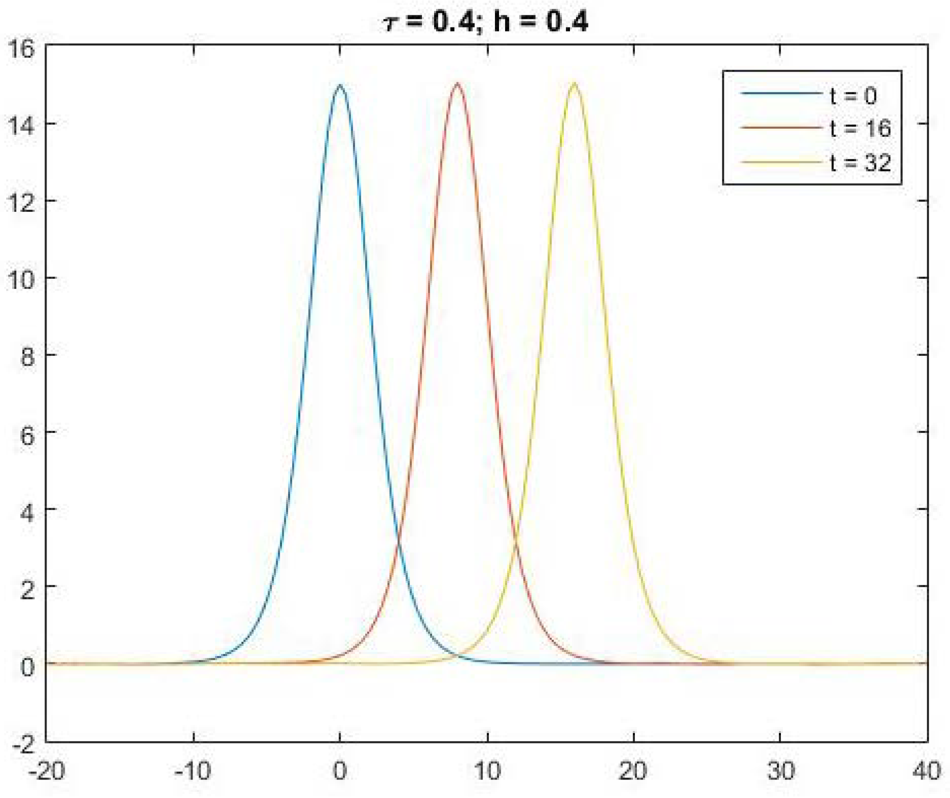
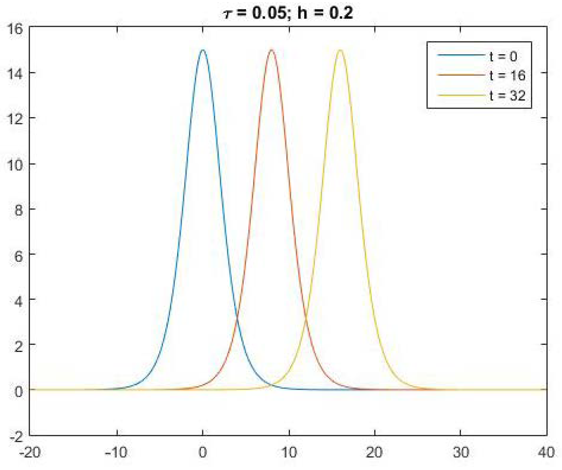
5. Numerical Experiments

If we take $\alpha =6$ and $k=\sqrt{2}/4$, the corresponding solitary wave solution of the KdV Equation (1) is

$$\begin{array}{c}\hfill u(x,t)={\displaystyle \frac{1}{4}}sec{h}^2\left[{\displaystyle \frac{\sqrt{2}}{4}}(x-{\displaystyle \frac{1}{2}}t)\right],\end{array}$$

and the initial function of problem (2)–(4) is defined as

$$\begin{array}{c}\hfill u_0\left(x\right)={\displaystyle \frac{1}{4}}sec{h}^2\left({\displaystyle \frac{\sqrt{2}}{4}}x\right).\end{array}$$

Fix $x_L=-20$, $x_R=40$ and $T=32$. To test the theoretical accuracy of the numerical solutions of the difference scheme (7)–(9) under different norms, define

$$\begin{array}{ccc}& & order{l}_2={log}_2(\parallel e^n(h,\tau )\parallel /\parallel e^{8n}({\displaystyle \frac{h}{2}},{\displaystyle \frac{\tau }{8}})\parallel ),\hfill \\ & & order{l}_{\infty }={log}_2(\parallel e^n{(h,\tau )\parallel }_{\infty }/\parallel e^{8n}({\displaystyle \frac{h}{2}},{\displaystyle \frac{\tau }{8}}){\parallel }_{\infty }).\hfill \end{array}$$

For different $\tau$ and h, the error estimates and the verification of numerical solutions’ accuracy of the difference scheme (7)–(9) are listed in

Table 1. The error estimates of the numerical solution at different times for different $\tau$ and h.

	$\mathit{\tau }=3.2,\mathit{h}=0.8$		$\mathit{\tau }=0.4,\mathit{h}=0.4$		$\mathit{\tau }=0.05,\mathit{h}=0.2$
	$\parallel {\mathit{e}}^{\mathit{n}}\parallel$	$\parallel {\mathit{e}}^{\mathit{n}}{\parallel }_{\infty }$	$\parallel {\mathit{e}}^{\mathit{n}}\parallel$	$\parallel {\mathit{e}}^{\mathit{n}}{\parallel }_{\infty }$	$\parallel {\mathit{e}}^{\mathit{n}}\parallel$	$\parallel {\mathit{e}}^{\mathit{n}}{\parallel }_{\infty }$
t = 3.2	–	–	1.3157 × ${10}^{-3}$	5.5531 × ${10}^{-4}$	2.1406 × ${10}^{-5}$	8.8211 × ${10}^{-6}$
t = 6.4	1.1135 × ${10}^{-1}$	4.5588 × ${10}^{-2}$	1.6453 × ${10}^{-3}$	7.4362 × ${10}^{-4}$	2.6198 × ${10}^{-5}$	1.1337 × ${10}^{-5}$
t = 9.6	1.5820 × ${10}^{-1}$	6.9156 × ${10}^{-2}$	1.9591 × ${10}^{-3}$	9.8618 × ${10}^{-4}$	3.0740 × ${10}^{-5}$	1.4817 × ${10}^{-5}$
t = 12.8	2.0214 × ${10}^{-1}$	8.0950 × ${10}^{-2}$	2.3343 × ${10}^{-3}$	1.2369 × ${10}^{-3}$	3.6743 × ${10}^{-5}$	1.9569 × ${10}^{-5}$
t = 16.0	2.4357 × ${10}^{-1}$	1.0679 × ${10}^{-1}$	2.7560 × ${10}^{-3}$	1.4574 × ${10}^{-3}$	4.3512 × ${10}^{-5}$	2.2924 × ${10}^{-5}$
t = 19.2	2.8437 × ${10}^{-1}$	1.2064 × ${10}^{-1}$	3.2298 × ${10}^{-3}$	1.7029 × ${10}^{-3}$	4.9380 × ${10}^{-5}$	2.4631 × ${10}^{-5}$
t = 22.4	3.2398 × ${10}^{-1}$	1.3248 × ${10}^{-1}$	3.7477 × ${10}^{-3}$	2.0014 × ${10}^{-3}$	5.9378 × ${10}^{-5}$	3.2336 × ${10}^{-5}$
t = 25.6	3.6183 × ${10}^{-1}$	1.5395 × ${10}^{-1}$	4.1745 × ${10}^{-3}$	2.1108 × ${10}^{-3}$	6.5077 × ${10}^{-5}$	3.3226 × ${10}^{-5}$
t = 28.8	3.9812 × ${10}^{-1}$	1.6528 × ${10}^{-1}$	4.7112 × ${10}^{-3}$	2.3874 × ${10}^{-3}$	7.4561 × ${10}^{-5}$	3.9540 × ${10}^{-5}$
t = 32.0	4.3176 × ${10}^{-1}$	1.7444 × ${10}^{-1}$	5.3390 × ${10}^{-3}$	2.7774 × ${10}^{-3}$	8.2891 × ${10}^{-5}$	4.3216 × ${10}^{-5}$

and

Table 2. The numerical verification of theoretical accuracy $O({\tau }^2+h^6)$.

	${\mathit{orderl}}_2$			${\mathit{orderl}}_{\mathit{\infty }}$
	$\mathit{\tau }=\mathbf{3}.\mathbf{2}$	$\mathit{\tau }=\mathbf{0}.\mathbf{4}$	$\mathit{\tau }=\mathbf{0}.\mathbf{05}$	$\mathit{\tau }=\mathbf{3}.\mathbf{2}$	$\mathit{\tau }=\mathbf{0}.\mathbf{4}$	$\mathit{\tau }=\mathbf{0}.\mathbf{05}$
	$\mathit{h}=\mathbf{0}.\mathbf{8}$	$\mathit{h}=\mathbf{0}.\mathbf{4}$	$\mathit{h}=\mathbf{0}.\mathbf{2}$	$\mathit{h}=\mathbf{0}.\mathbf{8}$	$\mathit{h}=\mathbf{0}.\mathbf{4}$	$\mathit{h}=\mathbf{0}.\mathbf{2}$
t = 3.2	–	–	5.942	–	–	5.976
t = 6.4	–	6.081	5.973	–	5.938	6.035
t = 9.6	–	6.335	5.994	–	6.132	6.056
t = 12.8	–	6.436	5.989	–	6.032	5.982
t = 16.0	–	6.466	5.985	–	6.195	5.990
t = 19.2	–	6.460	6.031	–	6.147	6.111
t = 22.4	–	6.434	5.980	–	6.049	5.952
t = 25.6	–	6.438	6.003	–	6.189	5.989
t = 28.8	–	6.401	5.982	–	6.113	5.916
t = 32.0	–	6.338	6.009	–	5.973	6.006

, respectively.

Note that in Table 2, we only provide the order verification of spatial accuracy. In fact, because of the use of discretization of the average implicit difference in time, second-order accuracy is direct. Moreover, the definitions of error orders $order{l}_2$ and $order{l}_{\infty }$ also indicate that the validation of the sixth-order accuracy in space implies the results of the second-order accuracy in the temporal direction.

Meanwhile, numerical simulations for conservative quantities (5) and (6) are also shown in

Table 3. Conservative quantities (10) and (11) for different $\tau$ and h.

	$\mathit{\tau }=0.4,\mathit{h}=0.4$		$\mathit{\tau }=0.05,\mathit{h}=0.2$
	${\mathit{Q}}^{\mathit{n}}$	${\mathit{E}}^{\mathit{n}}$	${\mathit{Q}}^{\mathit{n}}$	${\mathit{E}}^{\mathit{n}}$
t = 0	1.4142123912	0.2357022604	1.4142124684	0.2357022604
t = 3.2	1.4160938190	0.2357022604	1.4142431545	0.2357022604
t = 6.4	1.4160300272	0.2357022604	1.4142408716	0.2357022604
t = 9.6	1.4160715005	0.2357022604	1.4142452148	0.2357022604
t = 12.8	1.4163743439	0.2357022604	1.4142508295	0.2357022604
t = 16.0	1.4164056443	0.2357022604	1.4142476000	0.2357022604
t = 19.2	1.4161496430	0.2357022604	1.4142420138	0.2357022604
t = 22.4	1.4158790080	0.2357022604	1.4142390517	0.2357022604
t = 25.6	1.4156623709	0.2357022604	1.4142358229	0.2357022604
t = 28.8	1.4155983199	0.2357022604	1.4142326146	0.2357022604
t = 32.0	1.4155092729	0.2357022604	1.4142314379	0.2357022604

.

In comparison with the two-level nonlinear scheme presented in [21], the proposed three-level linearized scheme demonstrates superior computational efficiency.

Table 4. Comparison of time consumption between scheme (7)–(9) and the scheme in [21].

	$\mathit{\tau }=0.2, \mathit{h}=0.2$	$\mathit{\tau }=0.1, \mathit{h}=0.1$	$\mathit{\tau }=0.05, \mathit{h}=0.05$
Scheme (7)–(9)	1.850 s	6.550 s	23.852 s
Scheme in [21]	6.375 s	22.502 s	91.864 s

presents a comprehensive comparison of computational time requirements for both schemes across various values of $\tau$ and h. The data reveal that the computational efficiency gap between the two schemes widens progressively as the mesh parameters $\tau$ and h decrease. This trend suggests that the proposed scheme offers increasingly significant time savings for longer simulation durations. These findings further substantiate the computational advantages of our proposed scheme over the nonlinear approach described in [21].

Next, consider another case with a smaller parameter, for example, $\alpha =0.1$, and other parameters are the same as in the example above. The waveforms of $u(x,t)$ generated by the scheme (7)–(9) with different $\tau$ and h are illustrated in Figure 1, Figure 2 and Figure 3. The waveforms at $t=16$ and 32 in Figure 2 and Figure 3 demonstrate a significant level of agreement with the waveforms at $t=0$, which also indicates the efficiency of the scheme.

Figure 1 clearly demonstrates the instability of the numerical solution obtained from the difference scheme (7)–(9) when employing the parameter values $\tau =3.2$ and $h=0.8$. This instability arises from the violation of the scheme’s convergence condition. Specifically, ${\displaystyle \frac{11·\left|\alpha \right|·C_u}{15}}·{\displaystyle \frac{\tau }{h}}<1$, where $C_u$ represents an undetermined theoretical constant. Nevertheless, as evidenced by Figure 2 and Figure 3, reducing the parameter ratio ${\displaystyle \frac{\tau }{h}}$ ensures the satisfaction of the convergence condition, thereby enabling the numerical solution to approach the exact solution.

6. Conclusions

In this paper, an average implicit difference scheme (7)–(9) for problem (2)–(4) is proposed, which can possess second-order and sixth-order theoretical accuracy in the temporal and spatial directions, respectively. Furthermore, the conserved quantities (5) and (6) are also simulated accurately. More importantly, this scheme is linearized, which can achieve substantial savings in computation time.

Furthermore, while the numerical scheme (7)–(9) proposed in this study demonstrates superior computational efficiency, the nonlinear numerical scheme presented in [21] exhibits distinct advantages, particularly in terms of achieving a better absolute error value compared to the three-level scheme. Consequently, enhancing the iteration efficiency through the integration of advanced techniques, such as Nesterov’s accelerated method [25,26] and natural transform iterative method [27], represents a promising research direction. Additionally, it should be noted that the spatial accuracy of the current scheme is limited to the second order. The implementation of higher-order temporal discretization techniques, including the Runge–Kutta method [28], constitutes an important aspect of our future research.

References

1. Korteveg, D.J.; de Vries, G. On the change of long waves advancing in a rectangular canal, and on a new type of long stationary waves. Philos. Mag. 1895, 39, 422–443. [Google Scholar] [CrossRef]
2. Gardner, C.S.; Greene, J.M.; Kruskal, M.D.; Miura, R.M. Method for solving the Korteweg-de Vries equation. Phys. Rev. Lett. 1967, 19, 1095–1097. [Google Scholar] [CrossRef]
3. Morikawa, G.K.; Swenson, E.V. Korteweg-de Vries equation for nonlinear hydromagnetic waves in a warm collision-free plasma. Phys. Fluids 1969, 12, 2090–2093. [Google Scholar]
4. Miura, R.M.; Gardner, C.S.; Kruskal, M.D. Korteweg-de Vries equation and generalizations.II. Existence of conservation laws and constants of motion. J. Math. Phys. 1968, 9, 1204–1209. [Google Scholar] [CrossRef]
5. Su, C.S.; Gardner, C.S. Korteweg-de Vries equation and generalizations. III. Derivation of the Korteweg-de Vries equation and Burgers equation. J. Math. Phys. 1969, 10, 536–539. [Google Scholar] [CrossRef]
6. Osborne, A.R. Nonlinear Fourier analysis for the infinite-interval Korteweg-de Vries equation I: An algorithm for the direct scattering transform. J. Comput. Phys. 1991, 94, 284–313. [Google Scholar] [CrossRef]
7. Olver, P.J. Applications of Lie Groups to Differential Equations; Springer: Berlin/Heidelberg, Germany, 1986. [Google Scholar]
8. Hereman, W.; Korpel, A.; Banerjee, P.P. A general physical approach to solitary wave construction from linear solutions. Wave Motion 1985, 7, 283–289. [Google Scholar] [CrossRef]
9. Sanz-Serna, J.M.; Christie, I. Petrov-Galerkin methods for nonlinear dispersive waves. J. Comput. Phys. 1981, 39, 94–102. [Google Scholar] [CrossRef]
10. Amein, N.K.; Ramadan, M.A. A small time solutions for the KdV equation using Bubnov-Galerkin finite element method. J. Egypt Math. Soc. 2011, 19, 118–125. [Google Scholar] [CrossRef]
11. Karczewska, A.; Rozmej, P.; Szczeciński, M.; Boguniewicz, B. Finite element method for extended KdV equations. Int. J. Appl. Math. Comput. Sci. 2016, 26, 555–567. [Google Scholar] [CrossRef]
12. Benkhaldoun, F.; Seaid, M. New finite-volume relaxation methods for the third-order differential equations. Commun. Comput. Phys. 2008, 4, 820–837. [Google Scholar]
13. Shen, Q. A meshless method of lines for the numerical solution of KdV equation using radial basis functions. Eng. Anal. Bound. Elem. 2009, 33, 1171–1180. [Google Scholar] [CrossRef]
14. Zabusky, N.J.; Martin, D.K. Interaction of “solitons” in a collisionless plasma and the recurrence of initial states. Phys. Rev. Lett. 1965, 15, 240–243. [Google Scholar] [CrossRef]
15. Wang, H.P.; Wang, Y.S.; Hu, Y.Y. An explicit scheme for the KdV equation. Chin. Phys. Lett. 2008, 25, 2335–2338. [Google Scholar]
16. Vliegenthart, A.C. On finite-difference methods for the Korteweg-de Vries equation. J. Eng. Math. 1971, 5, 137–155. [Google Scholar] [CrossRef]
17. Greig, I.S.; Morris, J.L. A hopscotch method for the Korteweg-de Vries equation. J. Comput. Phys. 1976, 20, 64–80. [Google Scholar] [CrossRef]
18. Shen, J.L.; Wang, X.Q.; Sun, Z.Z. The conservation and convergence of two finite difference schemes for KdV equations with initial and boundary value conditions. Numer. Math. Theor. Meth. Appl. 2020, 13, 253–280. [Google Scholar]
19. Wang, X.P.; Sun, Z.Z. A second order convergent difference scheme for the initial-boundary value problem of Korteweg-de Vires equation. Numer. Methods Partial. Differ. Equ. 2021, 37, 2873–2894. [Google Scholar] [CrossRef]
20. Zhang, X.H.; Zhang, P. A reduced high-order compact finite difference scheme based on proper orthogonal decomposition technique for KdV equation. Appl. Math. Comput. 2018, 339, 535–545. [Google Scholar] [CrossRef]
21. Guo, Z.; Wu, M.M.; Hu, J. A conservative difference scheme with sixth-order spatial accuracy for the KdV equation. J. Sichuan Univ. Nat. Sci. Ed. 2023, 60, 031006. (In Chinese) [Google Scholar]
22. Wang, T.; Guo, B.; Zhang, L. New conservative difference schemes for a coupled nonlinear Schrödinger system. Appl. Math. Comput. 2010, 217, 1604–1619. [Google Scholar]
23. Zhou, Y.L. Application of Discrete Functional Analysis to the Finite Difference Method; International Academic Publishers: Beijing, China, 1990. [Google Scholar]
24. Wang, T. Maximum norm error bound of a linearized difference scheme for a coupled nonlinear Schrödinger equations. J. Comput. Appl. Math. 2011, 235, 4237–4250. [Google Scholar]
25. Temimi, H.; Ben-Romdhane, M.; Baccouch, M.; Musa, M.O. A two-branched numerical solution of the two-dimensional Bratu’s problem. Appl. Numer. Math. 2020, 153, 202–216. [Google Scholar]
26. Kasenov, S.E.; Tleulesova, A.M.; Sarsenbayeva, A.E.; Temirbekov, A.N. Numerical solution of the Cauchy problem for the Helmholtz equation using Nesterov’s accelerated method. Mathematics 2024, 12, 2618. [Google Scholar] [CrossRef]
27. Khalil, M.M.; Rehman, S.U.; Ali, A.H.; Nawaz, R.; Belal, B. New modifications of natural transform iterative method and q-homotopy analysis method applied to fractional order KDV-Burger and Sawada–Kotera equations. Partial. Differ. Equ. Appl. Math. 2024, 12, 100950. [Google Scholar]
28. Abdul-Hassan, N.Y.; Kadum, Z.J.; Ali, A.H. An efficient third-order scheme based on Runge–Kutta and Taylor series expansion for solving initial value problems. Algorithms 2024, 17, 123. [Google Scholar] [CrossRef]
Figure 1. Numerical solutions of u ( x , t ) with τ = 3.2 ,   h = 0.8 .
Mathematics 13 01132 g001
Figure 2. Numerical solutions of u ( x , t ) with τ = 0.4 ,   h = 0.4 .
Mathematics 13 01132 g002
Figure 3. Numerical solutions of u ( x , t ) with τ = 0.05 ,   h = 0.2 .
Mathematics 13 01132 g003