Abstract
The aim of this work is to model the nonlinear dynamics of conservative oscillators, with restoring force originating from even-order potentials. In particular, we extend our previous findings on inverting the time-integral equation that arises in the solution of such dynamical systems, a task that is almost always intractable in exact form. This is faced and solved by approximating the restoring force with its Chebyshev series truncated to order five; such a quintication approach yields a quinticate oscillator, whose associated time-integral can be inverted in closed form. Our solution procedure is based on the quinticate oscillator coefficients, upon which a second-order polynomial is constructed, which appears in the time-integrand of the quinticate problem, and whose roots determine the expression of the closed-form solution, as well as that of its period. The presented algorithm is implemented in the Mathematica software and validated on some conservative nonlinear oscillators taken from the relevant literature.
Keywords:
modeling of conservative nonlinear systems; Duffing-type dynamical models; near-minimax approximation; elliptic integrals; symbolic and numerical simulation MSC:
33C45; 33E05; 34A05; 65L05; 65P10; 68W30
1. Introduction
This work focuses on the differential equations governing the nonlinear dynamics of conservative oscillators. The current goal is to analyze the oscillator as a theoretical tool, in its mathematical aspects, leaving to future studies the physical effects, such as non-autonomous forcing perturbations, friction, or dissipation. This does not detract from the importance of this study, which represents a necessary starting model for applied systems. In this way, we complete the theoretical presentation of the oscillators treated in [1,2,3,4,5,6,7] in the light of what has already been produced in [8], adapting our solution method to the problems arising from the restoring forces (2) and (3) treated here and gaining notable results in terms of approximation obtained.
Specifically, we will deal with restoring forces, which, being odd functions, satisfy a precise symmetry condition, and which will be approximated with Chebyshev series arrested at the fifth order, to allow the closed-form solution of the quinticate system obtained. The term ‘quinticate’ is adopted to indicate that the solution method includes a quintication step, where the original restoring force is replaced by an equivalent expression, given as a function of quintic terms [9,10,11].
We follow the approach introduced in [8]. However, the present work does not constitute a mere replica of the procedures used therein, since a different wave configuration is considered here, which has never been addressed before. The root pattern in Theorem 1 is new and generates periodic waves different from those studied previously. As a further result of considering this new configuration, the present work demonstrates, once again, the stability of our method, when the type of wave generated by the original oscillator varies.
Overall, our procedure revises, refines, and extends earlier results on exact analytic solutions of quintic oscillators [12,13,14,15,16] and related fifth-order Chebyshev models [9,10,17]. In particular, two are the main features, induced by the nature of the restoring forces, which are of interest in our research. First of all, the class of dynamical systems examined generates, through the fifth-order truncated Chebyshev series, oscillators not yet considered in the literature: the point is that the nature of the oscillations is determined not only by the degree, as erroneously stated in [14], but also by the sign and position of the roots of the associated potential function; in the present work, the latter indicate types of elliptic integrals different from those encountered in [8] and therefore inverted via elliptic functions not used in [8]. Second, the two models presented here are such that both the time-integral and related period and the motion-integral cannot be evaluated in closed form; hence, the quintic approximation provides a symbolic estimate of the period energy function, which is then compared with the asymptotic period estimate obtained using results in [18].
This article is organized as follows. In Section 2, we describe how to construct the quinticate form of the original oscillator, in a general case, and how to arrive at the time-integral equation associated with the quinticate oscillator. We show that the periodic solution to the latter equation is linked to the roots of a second-order polynomial, and we state and prove Theorem 1, which provides a solution and period in closed form, under a particular roots configuration. In Section 3, our new solution process is applied to two Duffing oscillator models, and validated both qualitatively and quantitatively; further wave configurations have been considered, and the method has been validated on them, in [8], of which this work is a completion. In Section 4, a concise step-by-step description of our resolution procedure is provided. The conclusions are drawn in Section 5, where some indications on future work, currently under development, are also provided.
Before ending this section, let us recall how the literature dedicated to nonlinear oscillatory problems is rich in different techniques and approaches. The introductory sections of works such as [8,9,11,16], just to name a few, contain a classification and a short discussion of many of these approaches. The class of Chebyshev Quintication methods, to which our procedure belongs, is briefly discussed in [11], where the advantages of using the Chebyshev series expansion of the restoring force are reported, in particular with respect to the Taylor series. Further motivations for the use of orthogonal Chebyshev polynomials are given, for example, in [8] and in the references therein, and will be highlighted in Section 2 and Section 3; for now, let us just recall their good numerical properties, in terms of error propagation, and the fact that they provide near-minimax approximations.
The mathematical complexity of the inversion of the elliptic integral that governs the time evolution of the quinticate system is also mentioned in [11]: with our method, we manage to overcome this complexity. A generalization to higher-order Chebyshev polynomials will be the subject of future work, since it involves the inversion of hyperelliptic integrals and a level of mathematical sophistication still under exploration.
2. General Quintic Oscillator
We are interested in differential models configured as initial value problems (IVPs):
with odd and positive initial displacement a such that without loss of generality, can also be assumed. In particular, we consider:
which respectively represent the dimensionless form of the Duffing harmonic oscillator [1,2] and an instance of the generalized Duffing oscillator [3,4,5,6,7].
The motion governed by (1), with restoring force (2) or (3), is periodic, and the particle satisfies
As shown in [8], finding implies solving a time-integral equation where:
The auxiliary function with simple zeroes in the cases of our interest, appears in the solution period too:
The inversion often involves unknown functions and, therefore, cannot provide the explicit description of the motion.
To obtain an exactly invertible time-integral, we construct a near-minimax approximation of in terms of fifth-order truncated Chebyshev series. For this aim, we use the change of variable to normalize on the interval and associate the original problem (1) with the following IVP:
The normalized restoring force is then expanded in Chebyshev series, truncated (or projected) at order five:
where are first-kind Chebyshev polynomials of integer order while coefficients result from integrating a weighted inner product [19]:
Formulae (8) and (9), where yield an efficient and easy-to-handle near-minimax approximation [8]. This follows from the properties of Chebyshev polynomials, which ensure that a Lipschitz continuous function admits, on its domain a unique representation in terms of an absolutely and uniformly convergent Chebyshev series:
where:
Depending on the regularity of one can assume that the coefficients decrease in magnitude rapidly enough to imply that equioscillates times on so that is a near-minimax approximation of [19].
Expressing the projected force in the monomial base, a quinticate IVP replaces (7):
where:
In more detail, the relations between the Chebyshev coefficients and the coefficients in quinticate form (10) are the following, where
Applying (4)–(5) to the quinticate force in (10), we can see that the squared solution of (10) follows from evaluating and then inverting the following elliptic integral:
where is a parabola of the form:
In detail, to arrive at (12), we applied (4)–(5) to (10), computing:
and employing the change of variable so that
The discriminant of parabola discarding the factor is:
Given the physical nature of the models under investigation, coefficients can be assumed to be such that
- This scenario has already been explored in [8] in the the following two cases:

Within this scenario, we can describe the solution to problem (10), and its period, in closed form: we state and prove it in Theorem 1.
Theorem 1.
is given by the Jacobi amplitude function inverse of in the sense that Finally, is the Jacobi cosine amplitude and is the Jacobi sine amplitude.
Under condition (17), the quinticate problem (10) has exact squared solution and exact period given by:
where:
being the two roots of the parabola defined in (13).
- denotes the complete elliptic integral of the first kind, is the elliptic modulus, and is the elliptic integral of the first kind:
Proof.
The time-integral (12) can be rewritten as follows:
The elliptic integral (23) can be evaluated using entry 3.147–5 of [20], which we recall here for ease of reading:
where:
Here, it is hence, turns out to be as in (21), while (23) becomes:
Through the inversion of in equality (25), it is possible to see that the explicit representation of the squared solution of (10) is indeed:
with a period given by:
□
3. Application to the Duffing Oscillators
For the original oscillator (1) with restoring force (2) or (3), the normalized force is respectively:
whose auxiliary function defined in (5) and function in (4) become:
where while respectively for (26), (27).
In both cases, the time-integral equation does not admit a closed-form representation of its primitive, due to the presence of the logarithm and the powers in the term appearing in Formula (28).
This is also a further justification for using the Chebyshev expansion, instead of the Taylor one. The latter, in fact, gives a good approximation only at points, unlike the global approximation provided by the Chebyshev polynomials: this point-specific feature would negatively affect the Taylor approximation of the logarithm in away from zero. Furthermore, the Taylor expansion of would be limited to degree higher degrees would require the use of high-order hypergeometric functions, making the level of complexity excessive, and definitely more expensive than that implied by our method.
- Here, the integrand in (9), yielding the Chebyshev coefficients takes the form
At this point, based on coefficients and using (14), we form the discriminant of the second-order polynomial and find that hypothesis (17) of Theorem 1 holds for the quinticate oscillators under study. This is shown in Figure 2 and Figure 3.
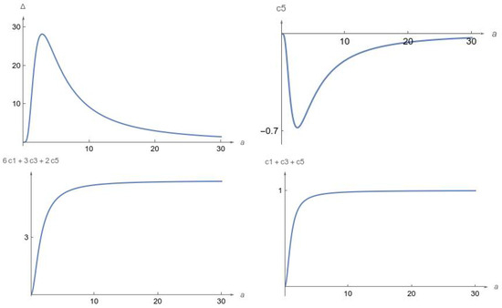
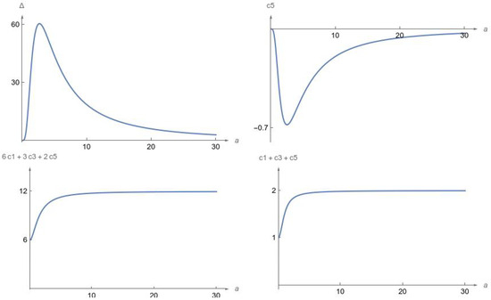
To deal with the elaborated expressions involved in condition (17), we developed our method and analysis within the Mathematica scientific environment [21,22], exploiting both symbolic and numeric resources, and graphics capabilities, sometimes in a hybrid manner [23,24].
The sought solution is the square root of (18), which we validated, qualitatively and quantitatively, through the differential operator:
whose behavior and maximum norm are studied in the first quarter of the period and for various values of the displacement
The quinticate oscillator is periodic and conservative, just like the original oscillator, and its solution and period are computed exactly using (18) and (19). Consequently, it suffices to study the differential operator (30) in the first quarter of the period, observing its deviation from zero, a value that would be obtained by applying (30) to the exact solution of the original oscillator.
Integration over longer time intervals is not an usual task in the case of periodic motion, where restarting is commonly performed after observing the motion for a period. This is also the motivation for using, if we want to numerically compute the solution of the original oscillator, an LSODE approach, namely, the Livermore Solver for Ordinary Differential Equations [25] available in Mathematica, equipped with switching between a non-stiff Adams method and a stiff Gear Backward Differentiation Formula method [26]; symplectic methods for long time integration, also available in Mathematica [27], are not needed here, and they go beyond the current scope of this research.
The period of the original oscillator can be numerically computed by integration, in which case a Gauss–Kronrod rule is used, by default, in one dimension: it consists in adaptive Gaussian quadrature, with error estimation based on evaluation at Kronrod points [28]; other methods, also available, are not necessary in the cases considered here.
Figure 4 shows a graph of the differential operator (30) applied to the quinticate oscillator associated with oscillator (1)–(2), at initial displacements In a similar way, Figure 5 plots the operator (30) for the quinticate form of oscillator (1)–(3), again at initial displacements
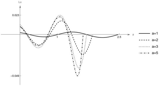
Figure 4.
Behavior of where is the square root of solution (18) for the quinticate form of the original oscillator (1)–(2). Here, what is significant is the deviation from zero: an upper bound is 0.048773 reached with from where a decrease can be observed. Also significative is the dependence of the behavior on the displacement .
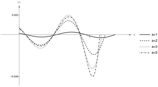
Figure 5.
Behavior of where is the square root of solution (18), for the quinticate form of the original oscillator (1)–(3). Here, what is significant is the deviation from zero: an upper bound is 0.048803 reached with from where a decrease can be observed. Also significative is the dependence of the behavior on the displacement .
As mentioned before, what is significant to observe in Figure 4 and Figure 5 is the deviation from zero. A small deviation indicates that the wave governed by the quinticate oscillator and the wave described by the original oscillator, although different, remain uniformly close to each other, and that both the quinticate and the original restoring forces cause the same physical effect. As expected, the behavior is worse initially due to the normalization of the integration interval, and improves with larger displacements. For any however, the differential operator remains bounded above, approximately by the machine-precision value
This is confirmed by the computation of the results of which are collected in Table 1 and Table 2, respectively, for the quinticate forms of oscillators (1)–(2) and (1)–(3), showing that the upper bound is reached at from where the norm of decreases monotonically. As for Figure 4 and Figure 5, also in Table 1 and Table 2, the small deviation from zero has the physical significance that the quinticate and original waves are uniformly close to each other.

Another measure that we introduced to validate the obtained solution is the ratio between the original oscillator period (6), computed via numerical quadrature, and the period of its quinticate form, obtained exactly from (19). This ratio remains close to and bounded above by a value smaller than as illustrated in Figure 6 for displacements up to and for both oscillators investigated.
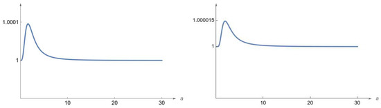
Figure 6.
Period ratio for the quinticate form of the original oscillator (1)–(2) in the left figure, and for the quinticate form of the original oscillator (1)–(3) in the right figure. The ratio compares the numerically evaluated period (6) of the original oscillator and the exactly evaluated period (19) of its quinticate form. Here, what is significant is the deviation from 1: the period ratio remains close to 1 in both cases, bounded above by 1.0001 in the case of oscillator (1)–(2), and bounded above by 1.000015 in the case of oscillator (1)–(3).
4. Pseudocode
For ease of reading and implementation, we provide here a concise description of the steps in our resolution procedure; the routines (in bold) mentioned are built-in functions available in Mathematica, version 14.0.
1– Choose the restoring force namely, (2) or (3), and normalize it as in (7) to obtain a function of the sought solution u and the displacement
2– Define the Chebyshev coefficients using (9):
where
- are computed exactly using Integrate, for example, and are functions of
3– Define the quinticate coefficients as functions of using (11):
4– Define the parabola which is a function of s and as in (13):
and compute its roots exactly using Solve, for example; are functions of
5– Form the discriminant as a function of as shown in (14):
and check that the conditions (17) are met so that Theorem 1 can be applied. This may be performed exploiting Reduce, for example, as well as the graphical capabilities of Mathematica.
6– Define the exact period of the quinticate oscillator, given by (19)–(20)–(21), namely:
EllipticK provides the complete elliptic integral of the first kind with the warning that it must be invoked as that is to say, using the squared elliptic modulus
- is a function of
7– Define the exact solution u of the quinticate oscillator as the square root of given by (18)–(20)–(21):
JacobiCN and JacobiSN provide the Jacobi cosine amplitude and the Jacobi sine amplitude, which must be invoked using the squared elliptic modulus
- u is a function of time t and the displacement
8– Evaluate the normalized restoring force defined in step 1, at the quinticate solution u obtained in step 7.
9– Form namely, the second derivative of the quinticate solution u with respect to using D, for example. is a function of time t and the displacement
10– Form the differential operator defined in (30), evaluating and at various values of the displacement a and for time
11– Define the period of the original oscillator as in (6), taking into account normalization, that is to say:
where is defined as in (5), again taking into account normalization, and is the normalized restoring force defined in step 1. Period T is a function of
12– Form the period ratio as the ratio between period of step 6 and period T defined in step 11 and numerically evaluated with NIntegrate, for example, for various values of the displacement
5. Conclusions and Future Work
With this work, we extend our previous findings on modeling the dynamics of non–dissipative and nonlinear oscillators, where the restoring force stems from even-order potentials and is, therefore, an odd function. Our attention, in particular, is directed to wave configurations that have not been considered before in the relevant literature.
In the case of the Duffing-type dynamical model examined here, of which (1)–(2) and (1)–(3) represent two common instances, an exact description of the motion would require a closed-form inversion of the associated time-integral, which is not feasible.
This is, instead, possible for the quinticate form of the original oscillator, obtained by fifth-order truncation of the Chebyshev series of the restoring force.
The core of our exact solution method is the construction of a parabola, which appears in the time-integral equation of the quinticate oscillator as a function of its coefficients, and whose root configuration constitutes the hypotheses of Theorem 1: the latter is new and guarantees the closed-form description of the motion and period of the quinticate differential problem, in terms of elliptic integrals of the first kind, thus invertible in the Jacobi sense.
We validate our method by comparing the solutions of the quinticate model and the original one, the latter taken in normalized form. This is performed by studying the qualitative behavior of the differential operator (30) and computing its uniform norm as a quantitative measure; the period ratio is also analyzed both qualitatively and quantitatively. All simulations performed confirm the efficiency of our new solution procedure.
Further work involves a generalization to truncations of order greater than five, which is currently being investigated and requires the inversion of hyperelliptic integrals, and related functionalities, that are under development although not yet available.
Author Contributions
Conceptualization, D.R.; methodology, D.R. and G.S.; software, G.S.; validation, G.S.; formal analysis, D.R.; investigation, D.R. and G.S.; resources, G.S.; data curation, D.R. and G.S.; writing—original draft preparation, D.R. and G.S.; writing—review and editing, G.S.; visualization, D.R. and G.S. All authors have read and agreed to the published version of the manuscript.
Funding
This research received no external funding.
Data Availability Statement
The original contributions presented in this study are included in the article. Further inquiries can be directed to the corresponding author(s).
Acknowledgments
The authors wish to thank Mark Sofroniou for many key discussions, as well as the editors and reviewers for their useful comments and assistance in improving the manuscript.
Conflicts of Interest
The authors declare no conflicts of interest.
References
- Mickens, R. Mathematical and numerical study of the Duffing–harmonic oscillator. J. Sound Vib. 2001, 244, 563–567. [Google Scholar] [CrossRef]
- Elias-Zuniga, A.; Martinez-Romero, O.; Cordoba-Diaz, R. Approximate solution for the Duffing-harmonic oscillator by the enhanced cubication method. Math. Probl. Eng. 2012, 2012, 12. [Google Scholar] [CrossRef]
- Beléndez, A.; Hernández, A.; Beléndez, T.; Alvarez, M.; Gallego, S.; Ortuno, M.; Neipp, C. Application of the harmonic balance method to a nonlinear oscillator typified by a mass attached to a stretched wire. J. Sound Vib. 2007, 302, 1018–1029. [Google Scholar]
- Zhao, L. He’s frequency–amplitude formulation for nonlinear oscillators with an irrational force. Comput. Math. Appl. 2009, 58, 2477–2479. [Google Scholar] [CrossRef]
- Jamshidi, N.; Ganji, D. Application of energy balance method and variational iteration method to an oscillation of a mass attached to a stretched elastic wire. Curr. Appl. Phys. 2010, 10, 484–486. [Google Scholar] [CrossRef]
- Younesian, D.; Askari, H.; Saadatnia, Z.; KalamiYazdi, M. Analytical approximate solutions for the generalized nonlinear oscillator. Appl. Anal. 2012, 91, 965–977. [Google Scholar]
- Marion, J. Classical Dynamics of Particles and Systems; Academic Press: New York, NY, USA, 2013. [Google Scholar]
- Boschi, M.; Ritelli, D.; Spaletta, G. Exact time–integral inversion via Chebyshev quintic approximations for nonlinear oscillators. J. Math. Anal. Appl. 2024, 533, 128015. [Google Scholar]
- Elias-Zuniga, A. Quintication method to obtain approximate analytical solutions of non–linear oscillators. Appl. Math. Comput. 2014, 243, 849–855. [Google Scholar]
- Big-Alabo, A. Approximate period for large–amplitude oscillations of a simple pendulum based on quintication of the restoring force. Eur. J. Phys. 2019, 41, 015001. [Google Scholar]
- Big-Alabo, A.; Ekpruke, E.; Ossia, C. Quasi-static quintication method for periodic solution of strong nonlinear oscillators. Sci. Afr. 2021, 11, e00704. [Google Scholar]
- Citterio, M.; Talamo, R. The elliptic core of nonlinear oscillators. Meccanica 2009, 44, 653. [Google Scholar] [CrossRef]
- Mingari Scarpello, G.; Ritelli, D. Exact solution to a first–fifth power nonlinear unforced oscillator. Appl. Math. Sci. 2010, 4, 3589–3594. [Google Scholar]
- Elias-Zuniga, A. Exact solution of the cubic–quintic Duffing oscillator. Appl. Math. Model. 2013, 37, 2574–2579. [Google Scholar]
- Beléndez, A.; Beléndez, T.; Martinez, F.; Pascual, C.; Alvarez, M.; Arribas, E. Exact solution for the unforced Duffing oscillator with cubic and quintic nonlinearities. Nonlinear Dyn. 2016, 86, 1687–1700. [Google Scholar] [CrossRef]
- Beléndez, A.; Arribas, E.; Beléndez, T.; Pascual, C.; Gimeno, E.; Álvarez, M. Closed–Form Exact Solutions for the Unforced Quintic Nonlinear Oscillator. Adv. Math. Phys. 2017, 2017, 7396063. [Google Scholar]
- Jonckheere, R. Determination of the period of nonlinear oscillations by means of Chebyshev polynomials. Z. Angew. Math. Mech. 1971, 51, 389–393. [Google Scholar] [CrossRef]
- Foschi, S.; Mingari Scarpello, G.; Ritelli, D. Higher order approximation of the period–energy function for single degree of freedom Hamiltonian systems. Meccanica 2004, 39, 357–368. [Google Scholar]
- Trefethen, L. Approximation Theory and Approximation Practice; SIAM: Philadelphia, PA, USA, 2019. [Google Scholar]
- Gradshteyn, I.; Ryzhik, J. Table of Integrals, Series and Products, 6th ed; Academic Press: New York, NY, USA, 2000. [Google Scholar]
- Wolfram, S. An Elementary Introduction to the Wolfram Language, 3rd ed.; Wolfram Media, Inc.: Champaign, IL, USA, 2023. [Google Scholar]
- WRI. Mathematica Quick Revision History. 2025. Available online: https://www.wolfram.com/language/quick-revision-history/ (accessed on 30 January 2025).
- Sofroniou, M. Symbolic derivation of Runge–Kutta methods. J. Symb. Comput. 1994, 18, 265–296. [Google Scholar] [CrossRef]
- Sofroniou, M.; Spaletta, G. Hybrid solvers for composition and splitting methods. J. Comput. Appl. Math. 2006, 185, 278–291. [Google Scholar]
- Hindmarsh, A. ODEPACK: A Systematized Collection of ODE Solvers. In Scientific Computing; Stepleman, R.S., Carver, M., Peskin, R., Ames, W.F., Vichnevetsky, R., Eds.; North Holland: Amsterdam, The Netherlands, 1983; pp. 55–64. [Google Scholar]
- Petzold, L. Automatic Selection of Methods for Solving Stiff and Nonstiff Systems of Ordinary Differential Equations. SIAM J. Sci. Stat. Comput. 1983, 4, 136–148. [Google Scholar] [CrossRef]
- Sofroniou, M.; Spaletta, G. Extrapolation Methods in Mathematica. J. Numer. Anal. Ind. Appl. Math. 2008, 3, 105–121. [Google Scholar]
- Monegato, G. Some remarks on the construction of extended Gaussian Quadrature Rules. Math. Comput. 1978, 32, 247–252. [Google Scholar]
Disclaimer/Publisher’s Note: The statements, opinions and data contained in all publications are solely those of the individual author(s) and contributor(s) and not of MDPI and/or the editor(s). MDPI and/or the editor(s) disclaim responsibility for any injury to people or property resulting from any ideas, methods, instructions or products referred to in the content. |
© 2025 by the authors. Licensee MDPI, Basel, Switzerland. This article is an open access article distributed under the terms and conditions of the Creative Commons Attribution (CC BY) license (https://creativecommons.org/licenses/by/4.0/).