Is π a Chaos Generator?

Abstract

We consider a circular motion problem related to blind search in confined space. A particle moves in a unit circle in discrete time to find the escape channel and leave the circle through it. We first explain how the exit time depends on the initial position of the particle when the channel width is fixed. We then investigate how narrowing the channel moves the system from discrete changes in the exit time to the ultimate ‘countable chaos’ state that arises in the problem when the channel width becomes infinitely small. It will be shown in the paper that inherent randomness exists in the problem due to the nature of circular motion as the number $\pi$ acts as a random number generator in the system. Randomness of the decimal digits of $\pi$ results in sensitive dependence on initial conditions in the system with an infinitely narrow channel, and we argue that even a simple linear dynamical system can exhibit features of chaotic behaviour, provided that the system has inherent noise.

1. Introduction

Uninformed (blind) search strategies present a wide class of search problems where no information about the search domain is available [1]. Those strategies provide basic search techniques to explore problems in which additional knowledge cannot be obtained beyond the definition of the problem. Blind search algorithms solve a wide range of problems in artificial intelligence, such as pathfinding, puzzle solving, and state-space search; see, e.g., [2,3,4]. Their applications also include various problems in astronomy [5], image processing [6], computational biology [7], animal foraging [8], etc.

While uninformed search refers to diversity of cases in different (i.e., spatial and non-spatial) search domains [9,10], various blind search techniques share several measures of their efficiency among which are completeness and time complexity. The completeness criterion asks the question: “Can we find a solution, if it exists?”, while the time complexity criterion asks: “How long does it take to find a solution?”. Search problems that have a deceptively simple formulation may demonstrate very complex properties when the above criteria of efficient search are applied, and one such problem is presented in this paper.

In our work, we consider an uninformed search problem in a spatial domain: a particle moves step by step along a unit circle to find the escape channel and exit through it. Discrete motion in a unit circle to find an escape channel can be classified as a blind search in confined space problem where an idealised setting we deal with implies a very simple and straightforward search algorithm which cannot be optimised, e.g., by making the particle’s step size variable. On the other hand, the particle’s motion can be considered as a discrete time linear dynamical system, and that system exhibits interesting and unusual properties when the completeness and time complexity criteria of the blind search are investigated. We demonstrate in the paper that while the exit time (that is, the search time) remains finite for any initial position of the particle, it experiences random jumps when an initial position of the particle is slightly changed. The incompatibility between the distance that the particle covers moving step by step and the circumference length generates noise responsible for unpredictable changes in the exit time. The noise in the system is inherent and cannot be suppressed because the number $\pi$ acts as a random number generator in the problem. Furthermore, narrowing the escape channel moves the system from discrete changes in the exit time to the state where the system becomes extremely sensitive to initial conditions as the channel width becomes infinitely small.

Since the problem can be studied in the framework of a discrete time linear dynamical system, its sensitivity to initial conditions is of particular interest, as this property is often considered the hallmark of chaotic dynamics [11,12]. Mathematicians are concerned with a rigorous definition of chaos, where sensitive dependence on initial conditions is a necessary but not sufficient requirement to conclude that a dynamical system is chaotic [13,14,15,16,17]. Meanwhile, detection and quantification of chaos in applied problems is often based on investigation of sensitivity alone [18,19] where conventional analysis of sensitivity to initial conditions employs calculation of Lyapunov exponents to measure the distance between two nearby solutions. A dynamical system that has at least one positive Lyapunov exponent is considered chaotic as nearby trajectories diverge exponentially with time and their evolution becomes unpredictable [20,21,22].

The analysis of Lyapunov exponents is widely employed by applied scientists (see, e.g., [23,24,25,26,27,28] among many other works), yet it does not allow us to estimate the divergence rate of trajectories in our problem since the maximal Lyapunov exponent is $\lambda =0$ in a linear dynamical system we deal with. The above result implies that if we have sensitive dependence on initial conditions, then nearby trajectories diverge slower than exponentially (cf. the discussion of ‘weak chaos’ in e.g., [29,30,31]) and it will be argued in the paper that trajectories diverge linearly when their rate of divergence is measured in terms of random jumps in the exit time. In the extreme case of an infinitely narrow channel, the system has sensitive dependence on initial conditions, which will be called countable chaos in the paper: any two trajectories separated initially by a small distance will be separated by an arbitrary large distance over time in the problem.

This paper is organised as follows. In Section 2, we formulate a blind search problem when a particle moves in a unit circle in discrete time. We then explain how to analyse the exit time as a function of the initial position of the particle in Section 3. Our analysis is essentially based on the concept of generating points, which is studied in detail in Section 4. Then in Section 5 it is argued that the analytical results obtained in the previous sections should be backed by computer simulation to efficiently address the question of the exit time, and we present a computational algorithm used to find the exit time for any initial condition taken from the domain of definition. In Section 6, we explain the random nature of jumps in the exit time and demonstrate the increasing unpredictability of the system when the channel narrows. We then investigate how the system will respond when the channel width becomes infinitely small in Section 7, where the concept of countable chaos is introduced. Conclusions, a brief analysis of the results, and suggestions for future work are provided in Section 8.

2. Problem Statement

We consider a particle moving along a unit circle parametrised by the angle $\varphi$. The circle has an ‘escape channel’ whose centre is positioned at $\varphi =\pi$ and the channel half-width is $\delta \in (0,\pi )$; see Figure 1a. In the rest of this paper, we assume that the channel half-width $\delta$ is sufficiently small (see Section 4.2 for a more accurate definition of $\delta$).

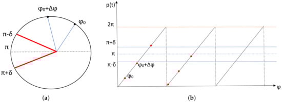
Figure 1. (a) A particle moving around a unit circle. The circle is parameterised by the angle $\varphi$ and the particle starts its movement at $\varphi ={\varphi }_0$. The centre of the escape channel of the width $2\delta$ is positioned at $\varphi =\pi$. (b) An example of a periodic trajectory of the particle, where the particle is shown as a closed red circle at every time $t=1,2,3\dots$. The position of the particle changes according to (3) until the particle leaves the domain through the escape channel.

While in the original problem statement [32] the particle was positioned at ${\varphi }_0=0$ at the time $t=0$, here we assume that the particle starts its movement from some location ${\varphi }_0$, where

$$0\le {\varphi }_0<\pi -\delta ={\varphi }_{max}.$$

(1)

The movement of the particle is discrete; i.e., the position of the particle has a constant increment $\Delta \varphi \in \mathbb{R}$ every next time $t=1,2,3\dots$, where we require $\Delta \varphi >2\delta$. Hence, the angle $\varphi$ is changed with time as

$$\varphi \left(t\right)=t\Delta \varphi +{\varphi }_0,t\in \mathbb{N},$$

(2)

and the problem can be considered as a discrete time dynamical system defined by the following linear map:

$${\varphi }_{t+1}={\varphi }_t+\Delta \varphi ,t=0,1,2,\dots$$

(2a)

where ${\varphi }_t\equiv \varphi \left(t\right)$ and ${\varphi }_0$ satisfies (1).

It is worth noting here that the definition of a ‘particle’ we employ in our model of circular motion is generic as a simple setting (1) and (2) considered in the paper is not related to any specific problem in physics, engineering, biology, etc. Focusing on a specific application may require different terminology, e.g., there is a spatial ‘profitable patch’ instead of an ‘escape channel’ if an animal’s foraging problem is considered, yet the problem formulation (1)–(2) remains the same and we therefore use the term ‘particle’ throughout the paper for the sake of convenience (but see the discussion in Section 8).

The discrete trajectory (2) of the particle can be presented as a set of equidistant points positioned along straight lines with slope $\Delta \varphi$. The position $p\left(t\right)$ of the particle is defined at the time t as

$$p\left(t\right)=\left\{\begin{array}{cc}\varphi \left(t\right),if\varphi \left(t\right)<2\pi ,& \\ \varphi \left(t\right)-2\pi ,if\varphi \left(t\right)\ge 2\pi ,& \end{array}\right.$$

(3)

where $\varphi \left(t\right)$ is given by (2); see Figure 1b. The particle is said to exit the circle at the time $t_e$ if it arrives at the escape channel at that time; i.e., the particle’s position is

$$\pi -\delta \le p\left(t_e\right)\le \pi +\delta ,$$

(4)

after making $t_e$ steps. The purpose of our study is to understand how the exit time $t_e$ depends on the initial position ${\varphi }_0\in [0,{\varphi }_{max})$ of the particle.

For the sake of our discussion, it is more convenient to consider an alternative representation of the circular motion (3). That is, we consider a single straight line $p\left(t\right)=\varphi \left(t\right)$ and place the channel centre at the points $n\pi$, $n=2k-1$, where $k\in \mathbb{N}$ is the channel number, as shown in Figure 2. Also, while the number of channels can be infinitely large, in some cases we will consider a system of N channels, where $N\in \mathbb{N}$ is a finite number; i.e., we will assume that the particle stops moving forever if it cannot exit the circle through one of the first N channels.

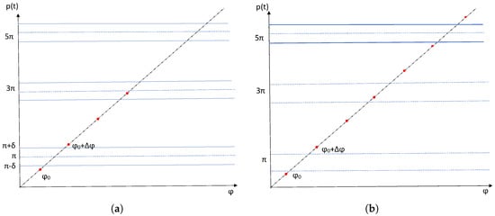
Figure 2. (a) A sweep of the periodic trajectory. The particle shown as a red closed circle escapes the domain through the second channel located at $3\pi$. (b) An example of the system under the assumption that all channels but one are ‘closed’. The position of each closed channel is indicated by blue dashed lines, while the open channel located at $5\pi$ is shown by bold blue lines. In the original system, the particle would escape through the second channel (cf. Figure 2a), but this channel is now closed and the particle continues moving along the trajectory. The third channel is open, yet the particle cannot exit through it.

The exit condition (4) is written for the system with many channels as follows:

$$\mid t_e\Delta \varphi +{\varphi }_0-n\pi \mid \le \delta .$$

(5)

In the next section, we will investigate the exit condition (5) under the assumption that all but one channels are ‘closed’; i.e., the particle can only exit the domain through the k-th channel located at $n\pi$. The above assumption will allow us to find the solution $t_e\left({\varphi }_0\right)$ to inequality (5), and the results obtained for the system with a single channel will then be generalised to a system where all channels are open.

3. The Escape Through the $\mathit{k}$-th Channel

The assumption about all channels but one being ‘closed’ we made at the end of the previous section means that we now consider the system with a single channel numbered as the k-th channel in the original system. The difference between the system with N channels and the system with a single channel is illustrated in Figure 2. The particle would escape through the second channel in the original system in Figure 2a where all channels are open. Meanwhile, the second channel is closed in the new system with a single channel; see Figure 2b. The particle cannot escape through the second channel in Figure 2b and continues moving along the trajectory. The only channel remaining open in the example in Figure 2b is the third channel, but the particle cannot exit through it and will move in the circle forever.

Consider the exit condition (5) and fix the half-width of the channel $\delta$ and the channel number k. Our aim is to find where the particle must be placed at the time $t=0$ to escape the domain if the k-th channel is the only channel open in the system. For the k-th channel located at $n\pi$ (where $n=2k-1$), we define $C_1=1/\Delta \varphi >0$, $C_2=(n\pi -\delta )/\Delta \varphi >0$, and $C_3=C_2+2\delta C_1>0$. The exit condition (5) becomes

$$-C_1{\varphi }_0+C_2\le t_e\le -C_1{\varphi }_0+C_3,$$

(6)

where $t_e\in \mathbb{N}$. In the following, we provide the solution to the inequalities (6) in terms of the function $t_e\left({\varphi }_0\right)$.

3.1. Finding the Time $t_e$ Required to Escape Through the k-th Channel

The inequalities (6) can be rewritten as

$$l_1(n,{\varphi }_0)\le t_e\le l_2(n,{\varphi }_0),$$

(7)

where $l_1(n,{\varphi }_0)=-C_1{\varphi }_0+C_2$ and $l_2(n,{\varphi }_0)=-C_1{\varphi }_0+C_3$ are linear functions of the variable ${\varphi }_0$. Let the exit time through the k-th channel be $t_e=m\left(n\right)$, where $m\left(n\right)\in \mathbb{N}$. The graphic representation of the conditions (7) is provided in Figure 3, where we show the range of the initial condition ${\varphi }_0\in [{\varphi }_0^l(m,n),{\varphi }_0^r(m,n)]$ for which the particle escapes the domain at time $m\left(n\right)$ through the channel located at $n\pi$.

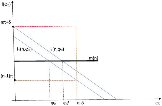
Figure 3. The graphic representation of the inequalities (7). The argument ${\varphi }_0^l$ in the function $l_1(n,{\varphi }_0)$ defines the left endpoint of the interval $[{\varphi }_0^l(m,n),{\varphi }_0^r(m,n)]$ where the exit time is $t_e=m$ if the particle is placed anywhere in $[{\varphi }_0^l(m,n),{\varphi }_0^r(m,n)]$ at the time $t=0$. The argument ${\varphi }_0^r$ in the function $l_2(n,{\varphi }_0)$ defines the right endpoint of the same interval. Since the values of ${\varphi }_0$ are bounded by ${\varphi }_{max}=\pi -\delta$ (red dashed vertical line in the graph), the interval where integer numbers $m\left(n\right)$ are considered is given by $\left[\right(n-1)\pi ,n\pi +\delta ]$ (see red dashed horizontal lines in the figure).

The left endpoint of the interval ${\varphi }_0^l(m,n)$ can be found from the following condition (see Figure 3):

$$l_1(n,{\varphi }_0)=m\left(n\right).$$

(8)

Rearranging terms, we obtain

$${\varphi }_0^l(m,n)={\displaystyle \frac{C_2-m\left(n\right)}{C_1}}.$$

(9)

Similarly, we require $l_2(n,{\varphi }_0)=m\left(n\right)$ to find the right endpoint ${\varphi }_0^r(m,n)$ as shown in Figure 3. We have

$${\varphi }_0^r(m,n)={\displaystyle \frac{C_3-m\left(n\right)}{C_1}}={\varphi }_0^l(m,n)+2\delta .$$

(10)

In the rest of this paper we consider the step size $\Delta \varphi =1$, although our analysis can be readily extended to another choice of $\Delta \varphi$. Substituting $\Delta \varphi =1$ into (9) and (10) gives us ${\varphi }_0^l(m,n)$ and ${\varphi }_0^r(m,n)$ as follows:

$${\varphi }_0^l(m,n)=n\pi -\delta -m\left(n\right),{\varphi }_0^r(m,n)=n\pi +\delta -m\left(n\right).$$

(11)

Since the initial position of the particle is bounded by conditions (1), we have to impose additional constraints on the left and right endpoints as follows:

$$\begin{array}{cc}{\varphi }_0^l(m,n)=0,\mathrm{if} n\pi -\delta -m\left(n\right)<0,& \\ {\varphi }_0^r(m,n)={\varphi }_{max},\mathrm{if} n\pi +\delta -m\left(n\right)\ge {\varphi }_{max}.& \end{array}$$

(12)

It is readily seen from (11) and (12) that the length of the interval $[{\varphi }_0^l(m,n),{\varphi }_0^r(m,n)]$ is always bounded as $|{\varphi }_0^r(m,n)-{\varphi }_0^l(m,n)|\le 2\delta$.

The exit time $m\left(n\right)$ that we have hypothesised in finding the interval $[{\varphi }_0^l(n,m),{\varphi }_0^r(n,m)]$ is not an arbitrary number $m\in \mathbb{N}$. The natural number m must be taken from a sequence $M_1,M_1+1,\dots ,M_2$, where the first term $M_1$ in the sequence is defined as

$$M_1=\lceil l_1(n,{\varphi }_{max})\rceil ,$$

(13)

and the function $\lceil ·\rceil$ is $\lceil x\rceil =min\{p\in \mathbb{Z}\mid p\ge x\}.$ Indeed, the condition (13) gives us the minimum $m\in \mathbb{N}$ for which the argument ${\varphi }_0$ in (9) is ${\varphi }_0<{\varphi }_{max}$; see Figure 3. Substituting $l_1(n,{\varphi }_0)$ and ${\varphi }_{max}$ into (13) and taking into account $\Delta \varphi =1$ results in

$$M_1=\lceil (n-1)\pi \rceil .$$

(14)

A similar approach can be employed to define $M_2$, where we have

$$M_2=\lfloor l_2(n,0)\rfloor ,$$

(15)

and the function $\lfloor ·\rfloor$ is $\lfloor x\rfloor =max\{p\in \mathbb{Z}\mid p\le x\}.$ The condition (15) provides us with the maximum $m\in \mathbb{N}$ for which the argument ${\varphi }_0$ in (10) is ${\varphi }_0>0$; see Figure 3. Substituting $l_2(n,0)$ into (15) gives

$$M_2=\lfloor n\pi +\delta \rfloor .$$

(16)

We note that $M_1=M_1\left(n\right)$ and $M_2=M_2\left(n\right)$; i.e., a sequence of exit times will be different if a different channel is considered.

Let us take two exit times m and $m+1$ from the sequence $M_1,M_1+1,\dots ,M_2$. It follows immediately from the definition (11) that for $\Delta \varphi =1$ the left endpoints ${\varphi }_0^l(m,n)$ and ${\varphi }_0^l(m+1,n)$ are related to each other as

$${\varphi }_0^l(m+1,n)={\varphi }_0^l(m,n)-1,$$

(17)

where the additional constraint (12) must be taken into account when $m+1=M_2$. We then calculate

$${\varphi }_0^r(m,n)={\varphi }_0^l(m,n)+2\delta ,$$

(18)

where we apply (12) if $m=M_1$. Hence, for the k-th channel, we have a union of the intervals ${\mathcal{R}}_k$,

$${\mathcal{R}}_k=[{\varphi }_0^l(M_2,n),{\varphi }_0^r(M_2,n)]\cup [{\varphi }_0^l(M_2-1,n),{\varphi }_0^r(M_2-1,n)]\cup \dots [{\varphi }_0^l(M_1,n),{\varphi }_0^r(M_1,n)],$$

defined by the point ${\varphi }_0^l(M_1,n)$, where $M_1=M_1\left(n\right)$ is given by (14). For any initial condition ${\varphi }_0\in {\mathcal{R}}_k$, the particle will escape through the k-th channel located at $n\pi$, $n=2k-1$, when all other channels are closed. Let us also define a complement ${\overline{\mathcal{R}}}_k=\mathcal{D}\setminus {\mathcal{R}}_k$, where $\mathcal{D}=[0,{\varphi }_{max})$. For any initial condition ${\varphi }_0\in {\overline{\mathcal{R}}}_k$, the particle will never escape through the k-th channel.

3.2. Example of the Graph $t_e\left({\varphi }_0\right)$

The following example illustrates the definition of the subdomain ${\mathcal{R}}_k$ in the domain of initial condition $\mathcal{D}=[0,{\varphi }_{max})$. Let the channel half-width and the step size be $\delta =0.1$ and $\Delta \varphi =1$, respectively. We consider $N=3$ (first three channels in the system) and compute the intervals $R_1$, $R_2$, $R_3$ corresponding to the escape through the first, second, and third channels, respectively. The results of the computation based on (17) and (18) are presented in Figure 4a, where the exit time $t_e$ is shown as a function of the initial position ${\varphi }_0$. We note that all sloped dashed lines in the figure correspond to those intervals along the ${\varphi }_0$-axis where the exit time is not defined; i.e., the particle cannot escape through any of the first three channels.

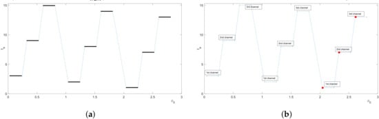
Figure 4. (a) The graph $t_e\left({\varphi }_0\right)$ for the channel half-width $\delta =0.1$: the exit time $t_e$ is shown as a function of the initial condition ${\varphi }_0$ when the particle escapes the domain through one of the first three channels. The exit time remains constant over each interval $[{\varphi }_0^l,{\varphi }_0^r]$. Sloped dashed lines in the graph correspond to the intervals along the ${\varphi }_0$-axis where the escape through any of the first three channels is not possible. (b) The points ${\varphi }_0^l(M_1\left(n\right),n)$, $n=1,3,5$ (red closed circles in the graph) belong to the same straight line and a regular structure of the graph $t_e\left({\varphi }_0\right)$ is entirely defined by the position of the point ${\varphi }_0^l(M_1\left(1\right),1)$ (red closed circle with the ‘1st channel’ label attached); see further explanation in the text.

The graph in Figure 4a is further explained in Figure 4b, where the channel number is shown for each exit time $t_e=const$. It can be seen from the figure that the intervals defining the escape through a given channel are located equidistantly along the ${\varphi }_0$-axis as they are computed according to (17) and (18). Furthermore, a visual inspection of Figure 4b reveals that the points ${\varphi }_0^l(M_1\left(n\right),n)$, $n=1,3,5$ shown as red closed circles in the graph belong to the same straight line, and we will provide a rigorous proof of this statement in the next section.

Let us introduce the distance between two consecutive channels $L_c=2\pi$ and the number of steps $\lfloor L_c\rfloor$ the particle takes over that distance when the step size is $\Delta \varphi =1$. Consider the escape through the second channel (i.e., $k=2$ and $n=3$) in the example above. The point ${\varphi }_0^l(M_1\left(3\right),3)$ is computed from (11) and (14) as follows:

$$\begin{array}{cc}{\varphi }_0^l(M_1\left(3\right),3)=3\pi -\delta -M_1\left(3\right)=3\pi -\delta -\lceil 2\pi \rceil =\pi -\delta +(2\pi -\lceil 2\pi \rceil )=& \\ \pi -\delta -1+(2\pi -\lfloor 2\pi \rfloor )={\varphi }_0^l(1,1)+L_G,& \end{array}$$

(19)

where the length $L_G$ is

$$L_G=2\pi -\lfloor 2\pi \rfloor =L_c-\lfloor L_c\rfloor .$$

(20)

Similarly, the escape through the third channel, where $k=3$ and $n=5$, gives the following result for ${\varphi }_0^l(M_1\left(5\right),5)$:

$$\begin{array}{cc}{\varphi }_0^l(M_1\left(5\right),5)=5\pi -\delta -M_1\left(5\right)=5\pi -\delta -\lceil 4\pi \rceil =\pi -\delta +(4\pi -\lfloor 4\pi \rfloor -1)=& \\ \pi -\delta -1+2(2\pi -\lfloor 2\pi \rfloor )={\varphi }_0^l(1,1)+2L_G,& \end{array}$$

(21)

where we have used $\lfloor 4\pi \rfloor =2\lfloor 2\pi \rfloor$.

Let us introduce the definition of a generating point in the system. We will say that the point ${\varphi }_0^l(m,n)$ is a generating point, ${\varphi }_0^l(m,n)\equiv {\varphi }_i^G$, $i=1,2,3\dots$, if

$${\varphi }_0^l(m,n)=n\pi -\delta -M_1\left(n\right)\mathrm{and}{\varphi }_0^l(m,n)\in [{\Phi }_1,{\Phi }_1+L_G],$$

(22)

where ${\Phi }_1=\pi -\delta -\Delta \varphi$, i.e., ${\Phi }_1=\pi -\delta -1$ for $\Delta \varphi =1$. We will also refer to the length $L_G$ given by (20) as the generating length. It is clear from the above discussion that the entire graph $t_e\left({\varphi }_0\right)$ in Figure 4 is produced by a single generating point ${\varphi }_1^G\equiv {\varphi }_0^l(M_1\left(1\right),1)$, where we have ${\varphi }_0^l(M_1\left(1\right),1)=\pi -\delta -1\equiv {\Phi }_1$. Given the point ${\varphi }_0^l(M_1\left(1\right),1)$, all the points $({\varphi }_0(m,n),t_e\left({\varphi }_0(m,n)\right)$ in the graph in Figure 4 can be calculated using the expressions (19) and (21) first (see the closed red circles in Figure 4b) and then applying (17) and (18).

Meanwhile, we have already seen that the graph $t_e\left({\varphi }_0\right)$ in Figure 4 does not have complete information about exit times when the number of channels is $N=3$. Hence, the number of channels must be increased to find the exit time for any ${\varphi }_0\in [0,{\varphi }_{max})$. We therefore want to understand what will happen to the regular structure of the graph generated by the point ${\varphi }_0^l(M_1\left(1\right),1)$ when we increase the number of channels in the system, and we will address this question in the next section.

4. Generating Points

In this section, we investigate the concept of generating points in more detail. We proceed with the example introduced in Section 3 where we now want to compute the exit time for channels with the number $k>3$. Since the length of each interval $[{\varphi }_0^l(m,n),{\varphi }_0^r(m,n)]$ is entirely defined by the position of the left endpoint ${\varphi }_0^l(m,n)$ (see Section 3), it is more convenient to deal with the graph $t_e\left({\varphi }_0^l(m,n)\right)$ instead of the graph $t_e\left({\varphi }_0\right)$ when a large number of channels are considered. Given the graph $t_e\left({\varphi }_0^l(m,n)\right)$, the graph $t_e\left({\varphi }_0\right)$ can be restored by defining ${\varphi }_0^r(m,n)$ from (18) and considering a constant exit time $t_e$ over each interval $[{\varphi }_0^l(m,n),{\varphi }_0^r(m,n)]$.

4.1. Example of Generating Points in the System

Let us increase the number of channels in the example in Section 3. The graph $t_e\left({\varphi }_0^l(m,n)\right)$ for $N=19$ is presented in Figure 5a, where the other parameters remain the same as in Figure 4. The graph is further explained in Figure 5b, where the point ${\varphi }_0^1(M_1\left(1\right),1)$ is now shown as a closed green circle with the 1(1) label attached. The point ${\varphi }_0^1(M_1\left(1\right),1)$ is a generating point which produces a regular grid $G_1$ sketched as red and magenta dashed lines in Figure 5b. The label attached to the generating point ${\varphi }_1^G\equiv {\varphi }_0^1(M_1\left(1\right),1)$ shows its number $i=1$ when a sequence of generating points is numbered and the channel number $k=1$ in brackets.

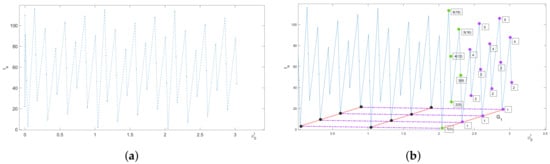
Figure 5. (a) The graph $t_e\left({\varphi }_0^l(m,n)\right)$. Each point ${\varphi }_0^l(m,n)$ shown as a blue closed circle in the graph is the left boundary of the interval $[{\varphi }_0^l(m,n),{\varphi }_0^r(m,n)]$ where the exit time $t_e$ remains constant. (b) Generating points shown as green closed circles in the graph $t_e\left({\varphi }_0^l(m,n)\right)$ produce regular grids in the $({\varphi }_0^l(m,n),t_e)$-plane. The grid $G_1$ produced by the first generating point (green closed circle with the 1(1) label attached) is shown as a collection of black closed circles corresponding to the exit through the same channel and magenta closed circles corresponding to the exit through the next channel (see further explanation in the text). As the channel number increases, new generating points appear in the system as indicated by the number attached to them along with the corresponding channel number in brackets. All magenta points related to the same generating point have the number of that generating point attached to demonstrate that grids defined by different generating points contain a different (unpredictable) number of nodes.

The grid $G_1$ is generated as follows. Consider the straight lines ${\mathit{L}}_{\mathit{1}}^{\mathit{1}}$ and ${\mathit{L}}_{\mathit{2}}^{\mathit{1}}$ starting at the generating point ${\varphi }_1^G\equiv {\varphi }_0^1(M_1\left(1\right),1)$ in the $({\varphi }_0^l(m,n),t_e)$-plane and defined as ${\mathit{L}}_{\mathit{1}}^{\mathit{1}}=-{\varphi }_0+{\varphi }_1^G+1$ and ${\displaystyle {\mathit{L}}_{\mathit{2}}^{\mathit{1}}=\frac{\lfloor 2\pi \rfloor }{2\pi -\lfloor 2\pi \rfloor }({\varphi }_0-{\varphi }_1^G)+1}$. The lines ${\mathit{L}}_{\mathit{1}}^{\mathit{1}}$ and ${\mathit{L}}_{\mathit{2}}^{\mathit{1}}$ have the direction vectors $\overrightarrow{v_1}$ and $\overrightarrow{v_2}$, respectively, where

$$\overrightarrow{v_1}=(-1,1),\overrightarrow{v_2}=(\lfloor 2\pi \rfloor ,2\pi -\lfloor 2\pi \rfloor ).$$

(23)

The increment ${\Delta }_1=-j_1\Delta \varphi$ given to the variable ${\varphi }_0^l(m,n)\in [0,{\varphi }_1^G]$ in the equation for the straight line ${\mathit{L}}_{\mathit{1}}^{\mathit{1}}$ produces grid points $j_1=0,1,2$, along the line ${\mathit{L}}_{\mathit{1}}^{\mathit{1}}$, where the point ${\varphi }_1^G$ corresponds to $j_1=0$ and $\Delta \varphi =1$ is the step size of the discrete movement of the particle. Those points define the exit through the same channel (i.e., the channel number is fixed) as explained in Section 3. They are shown as black closed circles in Figure 5b.

Similarly, the increment ${\Delta }_2=j_2{L}_G$ given to the variable ${\varphi }_0^l(m,n)\in [{\varphi }_1^G,{\varphi }_{max})$ starting from point ${\varphi }_1^G$ produces grid points $j_2=0,1,2,3$, along the straight line ${\mathit{L}}_{\mathit{2}}^{\mathit{1}}$. Those points are shown as closed magenta circles in Figure 5b, where the label attached to each point indicates that it belongs to the grid $G_1$. The grid points along the line ${\mathit{L}}_{\mathit{2}}^{\mathit{1}}$ define the exit through the next channel; i.e., the channel number increases by one when the next point $j_2$ is generated. The grid $G_1$ is then a tensor product of the one-dimensional grids in the $\overrightarrow{v_1}$- and $\overrightarrow{v_2}$- directions in the domain $0\le {\varphi }_0^l(m,n)<{\varphi }_{max}$; i.e., grid nodes are points of intersection between straight lines starting at points $j_1$ and $j_2$ and defined by the directed vectors $\overrightarrow{v_2}$ and $\overrightarrow{v_1}$, respectively (see the red and magenta dashed lines in Figure 5b).

If any $j_1\in \mathbb{Z}$ and $j_2\in \mathbb{Z}$ could be used in the definition of $G_1$, then an infinite grid G would be generated that covers the entire $({\varphi }_0,t_e)$-plane. However, the values of $j_1$ and $j_2$ have to be chosen as explained above due to the requirement that all points on the grid belong to the domain $[0,{\varphi }_{max})\times [0,\infty )$. Increasing the argument ${\Delta }_1=-j_1\Delta \varphi$, i.e., considering $j_1=3$, will result in a grid point outside the domain of definition as ${\varphi }_1^G-3\Delta \varphi <0$. Furthermore, we have $m=1,2,3$ for the channel number $k=1$ ($n=1$) in (17), so there are only three points positioned along the line ${\mathit{L}}_{\mathit{1}}^{\mathit{1}}$. Also, increasing the argument ${\Delta }_2=j_2{L}_G$, i.e., considering $j_2=4$, will produce a point that does not belong to the domain of definition as we have ${\varphi }_1^G+4L_G>{\varphi }_{max}$. Using the definition (11) gives ${\varphi }_0^l(M_1\left(9\right),9)=9\pi -\delta -M_1\left(9\right),$ and we obtain by simple algebraic transformation that

$$9\pi -\delta -M_1\left(9\right)=9\pi -\delta -\lceil 8\pi \rceil =\pi -\delta -1+(8\pi -\lfloor 8\pi \rfloor )\ne \pi -\delta -1+4(2\pi -\lfloor 2\pi \rfloor ),$$

where $\pi -\delta -1+4(2\pi -\lfloor 2\pi \rfloor )={\varphi }_1^G+4L_G$. The direct calculation reveals that the point ${\varphi }_0^1(M_1\left(9\right),9)$ is located within the same interval $[{\Phi }_1,{\Phi }_1+L_G]$ as the point ${\varphi }_0^1(M_1\left(1\right),1)$. Hence, the point ${\varphi }_0^1(M_1\left(9\right),9)$ is another generating point according to the definition (22).

The generating point ${\varphi }_2^G\equiv {\varphi }_0^1(M_1\left(9\right),9)$ is shown as a closed green circle along with the label 2(5) indicating the point number $i=2$ and the channel number $k=5$ in brackets in Figure 5b. This point generates a regular grid $G_2$ where the direction vectors are given by (23) and the grid step sizes ${\Delta }_1$ and ${\Delta }_2$ are the same as they are on the grid $G_1$, i.e., both grids $G_1$ and $G_2$ can be considered as sub-grids of the same infinite grid G generated when $j_1\in \mathbb{Z}$ and $j_2\in \mathbb{Z}$. The straight lines ${\mathit{L}}_{\mathit{1}}^{\mathit{2}}$ and ${\mathit{L}}_{\mathit{2}}^{\mathit{2}}$ on the grid $G_2$ start at the generating point ${\varphi }_2^G$; see Figure 5b. The grid points along the line ${\mathit{L}}_{\mathit{2}}^{\mathit{2}}$ are shown as closed magenta circles and the label attached to each point indicates that they belong to the grid $G_2$ (the other grid nodes on the grid $G_2$ are not shown for the sake of visualisation).

The grid $G_2$ contains again a finite number of nodes due to the restrictions imposed on the domain of definition. An analysis similar to that performed for the grid $G_1$ leads us to the conclusion that another generating point will appear in the system when the number of channels increases further. The third generating point then produces a grid $G_3$ and the number of generating points grows as the number of channels increases in the system; see Figure 5b, where the first six generating points are shown as closed green circles in the graph.

Our study of the example in this subsection results in two important conclusions. First, the entire graph $t_e\left({\varphi }_0^l(m,n)\right)$ can be considered as a union of grid points belonging to grids $G_i$, $i=1,2,3\dots$, where each grid $G_i$ is completely defined by its generating point. Second, each grid $G_i$ has a finite number of nodes, but that number is not the same. For example, the grid $G_1$ has 12 nodes, while the grid $G_3$ only has 9 nodes. Hence, we cannot assign some fixed numbers $j_1^{max}$ and $j_2^{max}$ to conclude that the transition from the current grid $G_i$ to the next grid $G_{i+1}$ will occur every time when $j_1=j_1^{max}$ and $j_2=j_2^{max}$. In the next subsection, we provide a proof of the statement that, given the step size $\Delta \varphi =1$, the number of grid nodes on any grid $G_i$, $i=1,2,3\dots$ can be 16 at most.

4.2. Analysis of Grid $G_i$

Let a grid $G_i$ be produced by a generating point ${\varphi }_i^G$, $i=1,2,3\dots$. Consider straight lines ${\mathit{L}}_{\mathit{1}}^{\mathit{i}}$ and ${\mathit{L}}_{\mathit{2}}^{\mathit{i}}$ starting at the generating point ${\varphi }_i^G$ in the $({\varphi }_0^l(m,n),t_e)$-plane. The line ${\mathit{L}}_{\mathit{1}}^{\mathit{i}}$ is defined as

$${\mathit{L}}_{\mathit{1}}^{\mathit{i}}=-{\varphi }_0+{\varphi }_i^G+1,$$

by the definition of the exit through the same channel. Hence, the directed vector $\overrightarrow{v_1}$ is the same as on the grid $G_1$ and is given by (23). Since we have ${\Phi }_1\le {\varphi }_i^G\le {\Phi }_1+L_G$ and ${\Phi }_1=\pi -\delta -1$, the minimum number $P_{mi{n}^1}$ of grid points along the line ${\mathit{L}}_{\mathit{1}}^{\mathit{i}}$ is $P_{mi{n}^1}=\lfloor {\Phi }_1+1\rfloor =3$, while the maximum number $P_{ma{x}^1}$ of grid points along the line ${\mathit{L}}_{\mathit{1}}^{\mathit{i}}$ is $P_{ma{x}^1}=\lceil {\Phi }_1+L_G+1\rceil =4$ for any sufficiently small channel half-width $\delta <\pi -\lfloor \pi \rfloor$.

Let us now demonstrate that the line ${\mathit{L}}_{\mathit{2}}^{\mathit{i}}$ is defined as

$${\mathit{L}}_{\mathit{2}}^{\mathit{i}}={\displaystyle \frac{\lfloor 2\pi \rfloor }{2\pi -\lfloor 2\pi \rfloor }}({\varphi }_0-{\varphi }_i^G)+1.$$

We first check that the grid points along the line ${\mathit{L}}_{\mathit{2}}^{\mathit{i}}$ on the grid $G_i$ are equidistant. Consider ${\varphi }_0^l(M_1\left(n\right),n)$, where $n=2k-1$ and $k\in \mathbb{N}$ is an arbitrary channel number. We want to find the distance between the points ${\varphi }_0^l(M_1(n+2),n+2)$ and ${\varphi }_0^l(M_1\left(n\right),n)$, where the point ${\varphi }_0^l(M_1(n+2),n+2)$ corresponds to the escape through the next channel $k+1$. Taking into account (11) and (14), we have

$$\begin{array}{cc}{\varphi }_0^l(M_1\left(n\right),n)=n\pi -\delta -\lceil (n-1)\pi \rceil =n\pi -\delta -\lfloor (n-1)\pi \rfloor -1,& \\ & \\ {\varphi }_0^l(M_1(n+2),n+2)=(n+2)\pi -\delta -\lceil (n+1)\pi \rceil =n\pi +2\pi -\delta -\lfloor (n+1)\pi \rfloor -1,\end{array}$$

(24)

and the distance between the two points is

$${\varphi }_0^l(M_1(n+2),n+2)-{\varphi }_0^l(M_1\left(n\right),n)=2\pi -\left(\lfloor (n+1)\pi \rfloor -\lfloor (n-1)\pi \rfloor \right).$$

We note that $\lfloor (n-1)\pi \rfloor =(n-1)\pi -d_{(n-1)\pi }$, where the fractional part of the number $(n-1)\pi$ is $d_{(n-1)\pi }\in \mathbb{R}$ and $0<d_{(n-1)\pi }<1$. Similarly, $\lfloor (n+1)\pi \rfloor =(n+1)\pi -d_{(n+1)\pi }$, where the fractional part $d_{(n+1)\pi }\in \mathbb{R}$ and $0<d_{(n+1)\pi }<1$. Hence, we introduce

$$J_n\equiv \lfloor (n+1)\pi \rfloor -\lfloor (n-1)\pi \rfloor =2\pi -d_{(n+1)\pi }+d_{(n-1)\pi }=\lfloor 2\pi \rfloor +d_{2\pi }-d_{(n+1)\pi }+d_{(n-1)\pi }=\lfloor 2\pi \rfloor +S_n,$$

where $S_n=d_{2\pi }-d_{(n+1)\pi }+d_{(n-1)\pi }$ and $d_{2\pi }=2\pi -\lfloor 2\pi \rfloor$. Gathering terms results in

$${\varphi }_0^l(M_1(n+2),n+2)-{\varphi }_0^l(M_1\left(n\right),n)=2\pi -\lfloor 2\pi \rfloor -S_n.$$

(25)

Since $J_n=\lfloor 2\pi \rfloor +S_n$ and $J_n\in \mathbb{N}$, we require $S_n\in \mathbb{Z}$. Given the bounds $0<d_{(n-1)\pi }<1$, $0<d_{(n+1)\pi }<1$, and $0.28<d_{2\pi }<0.29$, the value of $S_n$ can only be (A) $S_n=0$ or (B) $S_n=1$.

Let us first consider the case (A). Substituting $S_n=0$ into (25) results in

$${\varphi }_0^l(M_1(n+2),n+2)-{\varphi }_0^l(M_1\left(n\right),n)=2\pi -\lfloor 2\pi \rfloor =L_G.$$

Therefore, the point ${\varphi }_0^l(M_1(n+2),n+2)={\varphi }_0^l(M_1\left(n\right),n)+L_G$ belongs to the same straight line as the point ${\varphi }_0^l(M_1\left(n\right),n)$ (see discussion in Section 3) and ${\varphi }_0^l(M_1(n+2),n+2)$ is not a generating point.

Consider now case (B). We substitute $S_n=1$ into (25) to obtain

$${\varphi }_0^l(M_1(n+2),n+2)-{\varphi }_0^l(M_1\left(n\right),n)=2\pi -\lfloor 2\pi \rfloor -1=L_G-1.$$

Therefore, ${\varphi }_0^l(M_1(n+2),n+2)={\varphi }_0^l(M_1\left(n\right),n)+L_G-1$ does not belong to the same straight line as the point ${\varphi }_0^l(M_1\left(n\right),n)$. Furthermore, it follows from (24) that

$$\begin{array}{cc}{\varphi }_0^l(M_1(n+2),n+2)={\varphi }_0^l(M_1\left(n\right),n)+L_G-1=n\pi -\delta -\lfloor (n-1)\pi \rfloor -1+L_G-1& \\ =\pi -\delta -1+L_G-1+d_{(n-1)\pi }={\Phi }_1+L_G+(d_{(n-1)\pi }-1).& \end{array}$$

Since $d_{(n-1)\pi }<1$, we have ${\varphi }_0^l(M_1(n+2),n+2)<{\Phi }_1+L_G$ and therefore ${\varphi }_0^l(M_1(n+2),n+2)$ is another generating point in the system.

Let us now prove that there are at least $P_{mi{n}^2}=3$ and at most $P_{ma{x}^2}=4$ grid points positioned along the line ${\mathit{L}}_{\mathit{2}}^{\mathit{i}}$ on the grid $G_i$. Consider a generating point ${\varphi }_i^G\equiv {\varphi }_0^l(M_1\left(n\right),n)$. We have by the definition of generating point

$${\varphi }_i^G=n\pi -\delta -\lceil (n-1)\pi \rceil =\pi -\delta -1+\alpha \left(n\right),$$

(26)

where

$$0\le \alpha \left(n\right)=(n-1)\pi -\lfloor (n-1)\pi \rfloor \le L_G.$$

(27)

Consider now the exit through the next channel and let us check whether the point ${\varphi }_0^l(M_1(n+2),n+2)$ belongs to the grid $G_i$ generated by ${\varphi }_0^l(M_1\left(n\right),n)$. We require ${\varphi }_0^l(M_1(n+2),n+2)={\varphi }_0^l(M_1\left(n\right),n)+L_G$ for the point ${\varphi }_0^l(M_1(n+2),n+2)$ to be on the grid $G_i$. The boundary condition gives

$${\varphi }_0^l(M_1\left(n\right),n)+L_G=\pi -\delta -1+\alpha +L_G<{\varphi }_{max}=\pi -\delta ,$$

and therefore, we have

$$\alpha +L_G<1.$$

Since the generating length is $L_G=2\pi -\lfloor 2\pi \rfloor \equiv d_{2\pi }$, we have $0.28<L_G<0.29$. Hence, the above condition holds for any $\alpha \in [0,L_G]$ and the point ${\varphi }_0^l(M_1(n+2),n+2)$ always belongs to the grid $G_i$ generated by ${\varphi }_0^l(M_1\left(n\right),n)$.

Similarly, let us check whether the point ${\varphi }_0^l(M_1(n+4),n+4)$ belongs to the grid $G_i$, i.e., ${\varphi }_0^l(M_1(n+4),n+4)={\varphi }_0^l(M_1(n+2),n+2)+L_G={\varphi }_0^l(M_1\left(n\right),n)+2L_G$. Implementing the boundary condition gives

$$\pi -\delta -1+\alpha +2L_G<\pi -\delta \Rightarrow \alpha +2L_G<1.$$

Again, the above condition holds for any $\alpha \in [0,L_G]$.

Consider now ${\varphi }_0^l(M_1(n+6),n+6)$. Similar analysis gives

$$\pi -\delta -1+\alpha +3L_G<{\varphi }_{max}=\pi -\delta \Rightarrow \alpha +3L_G<1.$$

This condition holds for $\alpha \in [0,{\alpha }^{\ast })$, where ${\alpha }^{\ast }=1-3L_G=0.15044407\dots$ and is violated for any $\alpha \in [{\alpha }^{\ast },L_G]$. Hence, the point ${\varphi }_0^l(M_1(n+6),n+6)$ can belong to the grid $G_i$ generated by the point ${\varphi }_0^l(M_1\left(n\right),n)$ or can be another generating point. In the first case, the distance between ${\varphi }_0^l(M_1(n+4),n+4)$ and ${\varphi }_0^l(M_1(n+6),n+6)$ is $L_G$, and $S_n=0$, while in the latter case the distance between ${\varphi }_0^l(M_1(n+4),n+4)$ and ${\varphi }_0^l(M_1(n+6),n+6)$ is $L_G-1$, and $S_n=1$.

Let $\alpha \in [{\alpha }^{\ast },L_G]$, and then a new generating point appears at the interval $({\Phi }_1,{\Phi }_1+L_G)$. We have ${\Phi }_1<{\Phi }_1+\alpha +3L_G-1,$ as $\alpha +3L_G>1$ by choice of $\alpha \in [{\alpha }^{\ast },L_G]$. We also note that ${\Phi }_1+\alpha +3L_G-1={\Phi }_1+L_G+(\alpha +2L_G-1)<{\Phi }_1+L_G$ because $\alpha +2L_G<1$ always holds.

Finally, we check whether the point ${\varphi }_0^l(M_1(n+8),n+8)$ belongs to the grid $G_i$. We have

$$\pi -\delta -1+\alpha +4L_G<{\varphi }_{max}=\pi -\delta \Rightarrow \alpha +4L_G<1.$$

This condition is violated for any $\alpha \in [0,L_G]$ and we either conclude that ${\varphi }_0^l(M_1(n+8),n+8)$ is another generating point in the system (which occurs if ${\varphi }_0^l(M_1(n+6),n+6)$ is not a generating point) or ${\varphi }_0^l(M_1(n+8),n+8)$ belongs to the grid $G_{i+1}$ generated by point ${\varphi }_{i+1}^G\equiv {\varphi }_0^l(M_1(n+6),n+6)$.

We have shown that if ${\varphi }_0^l(M_1\left(n\right),n)$ is a generating point, then the points ${\varphi }_0^l(M_1\left(n\right),n)$, ${\varphi }_0^l(M_1(n+2),n+2)$, ${\varphi }_0^l(M_1(n+4),n+4)$ always belong to the line ${\mathit{L}}_{\mathit{2}}^{\mathit{i}}$, while the point ${\varphi }_0^l(M_1(n+6),n+6)$ either belongs to the line ${\mathit{L}}_{\mathit{2}}^{\mathit{i}}$ or becomes the next generating point. Hence, the maximum number $P_{ma{x}^2}$ of grid points along the line ${\mathit{L}}_{\mathit{2}}^{\mathit{i}}$ is $P_{ma{x}^2}=4$.

It is important to note that, while the number of points along the line ${\mathit{L}}_{\mathit{1}}^{\mathit{i}}$ depends on the parameter $\delta$, the number of points along the line ${\mathit{L}}_{\mathit{2}}^{\mathit{i}}$ is defined by the step size $\Delta \varphi$ and does not depend on the channel width. Furthermore, the condition $\alpha \left(n\right)>{\alpha }^{\ast }$ that defines the next generating point in the system depends on the value of n, as $\alpha =\alpha \left(n\right)$ in (27). We will argue in Section 6 that the above condition cannot be checked beforehand for each new n and therefore we cannot say a priori how the next grid $G_i$ is shifted with respect to the previous grid.

5. The System with $\mathit{N}$ Channels Open

Knowledge of generating points allows one to find where the particle has to be located at the time $t=0$ to leave the domain through the k-th channel. This question can be investigated for any $k\in \mathbb{N}$ and therefore the number of channels N can be arbitrary in the problem. However, the analysis in Section 3 and Section 4 has been made under the assumption that only the k-th channel is open for the particle’s escape through it, while the original problem statement demands that the particle can escape the domain through any channel. The definition of the number of channels N requires careful consideration when all channels are open in the system. Based on the results obtained in Section 3, in the following we explain how to obtain a solution to the escape problem with all channels open.

Given the number of channels N, we will say the total escape occurs in the system if the particle exits the domain through one of those channels, wherever the initial position of the particle ${\varphi }_0$ is within the domain $[0,{\varphi }_{max}]$. Clearly, if the total escape occurs for some $N=N_{min}$, then it will also occur for any $N>N_{min}$. Hence, our next goal is to define the minimum number of channels $N_{min}$ for which the total escape is ensured.

Let us introduce the escape range $P_e\left(N\right)$ as follows:

$$P_e\left(N\right)={\displaystyle \frac{1}{{\varphi }_{max}}}\sum _{k=1}^N{L}_{{\varphi }_0}\left(k\right),$$

(28)

where $L_{{\varphi }_0}\left(k\right)$ is a subdomain in the domain $[0,{\varphi }_{max})$ identified from the condition that the particle escapes through the k-th channel if its initial position is ${\varphi }_0\in L_{{\varphi }_0}\left(k\right)$. We then define the minimum number of channels $N_{min}$ required for the total escape from the following conditions:

$$P_e\left(N\right)<1 \mathrm{for} \mathrm{any} N<N_{min},and{P}_e\left(N_{min}\right)=1.$$

(29)

Unlike the ‘single channel’ problem in Section 3, the definition of $L_{{\varphi }_0}\left(k\right)$ in (28) now requires the analysis of intersection between intervals where the time $t_e$ remains constant to avoid overlapping of those intervals. An example of such overlap is shown in Figure 6a, where we sketch two hypothetical times $m_1\left(n_1\right)$ and $m_2\left(n_2\right)$ corresponding to the exit through the channels $k_1$ and $k_2>k_1$, respectively (cf. Figure 3). It is easily seen in the figure that we cannot consider the entire subdomain $[{\varphi }_0^l\left(m_2\right),{\varphi }_0^r\left(m_2\right)]$ as an interval where the particle has to be placed to leave the domain with the exit time $m_2$. The correct interval is now given by $[{\varphi }_0^r\left(m_1\right),{\varphi }_0^r\left(m_2\right)]$ and is highlighted in red along the ${\varphi }_0$-axis in Figure 6a. We also note that the subdomain $[{\varphi }_0^l\left(m_1\right),{\varphi }_0^r\left(m_2\right)]$ provides the exit time given by $m_1\left(n_1\right)$ or $m_2\left(n_2\right)$.

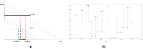
Figure 6. (a) Overlapping between intervals along the ${\varphi }_0$-axis corresponding to the exit times $m_1\left(n_1\right)$ and $m_2\left(n_2\right)$. The subdomain $[{\varphi }_0^l\left(m_1\right),{\varphi }_0^r\left(m_2\right)]$ should be considered to provide the exit time given by either $m_1\left(n_1\right)$ or $m_2\left(n_2\right)$; see Figure 3 for explanation of sloped lines $l\left({\varphi }_0\right)$. (b) The graph of the exit time $t_e$ as a function of the initial condition ${\varphi }_0$ for the channel half-width $\delta =0.1$. The number of channels required for the total escape is $N_{min}=7$, i.e., the particle will always exit the domain through one of the first $N=7$ channels, no matter what the initial position ${\varphi }_0\in [0,{\varphi }_{max})$ of the particle is. Each interval where the exit time remains constant has the length $2\delta$ at most.

The definition (28) and (29) can be illustrated by the baseline example introduced previously in Section 3. We have ${\varphi }_{max}=\pi -\delta =3.0415\dots$ for the channel half-width $\delta =0.1$. For the number of channels $N=3$ in the baseline example, there are nine intervals $[{\varphi }_0^l,{\varphi }_0^r]$ (i.e., three intervals for each channel) where the escape is possible if the particle’s initial position belongs to any of those intervals; see Figure 4. Since the length of each interval $[{\varphi }_0^l,{\varphi }_0^r]$ is $2\delta$ in the example of Figure 4, the size of the subdomain where escape is possible is ${\displaystyle \sum _{k=1}^N}{L}_{{\varphi }_0}\left(k\right)=9\left(2\delta \right)=18\delta =1.8$ when $\delta =0.1$ is considered in the definition (28). The same result can be obtained by noting that we have three subdomains $L_{{\varphi }_0}\left(1\right)$, $L_{{\varphi }_0}\left(2\right)$, and $L_{{\varphi }_0}\left(3\right)$ in the above example, where each subdomain $L_{{\varphi }_0}\left(k\right)$, $k=1,2,3$, consists of three equal intervals of length $2\delta$; see the explanation of $L_{{\varphi }_0}\left(k\right)$ in the definition (28). Substitution of ${\displaystyle \sum _{k=1}^N}{L}_{{\varphi }_0}\left(k\right)=1.8$ into (28) gives $P_e=0.5918\dots <1$ and therefore escape through any of the first three channels is not the total escape. This statement is supported by the graph in Figure 4 where we can see gaps in the domain of initial condition for which the exit time is not defined.

Consider now $N=19$ in the same example (see Section 4). Direct computation reveals that $P_e=1$ for $N=19$, yet this number of channels is $N\ne N_{min}$ as the total escape $P_e=1$ can also be achieved for a smaller number of channels, e.g., when we have $N=12$ or $N=9$. The accurate computation of $N_{min}$ is then based on the Algorithm 1.

Algorithm 1

Consider the channel number $k=1$. Let the domain $\mathcal{D}=[0,{\varphi }_{max})$ and the subdomain ${\mathcal{S}}_1=\varnothing$. Define $n=2k-1$. Find all subintervals $[{\varphi }_0^l,{\varphi }_0^r]$, where exit through the escape channel k is possible. $${\varphi }_0^l(m,n)=n\pi -\delta -m\left(n\right),{\varphi }_0^r(m,n)=n\pi +\delta -m\left(n\right),$$ where $m\left(n\right)\in \mathbb{N}:M_1\left(n\right)\le m\left(n\right)\le M_2\left(n\right)$, $M_1=\lceil (n-1)\pi \rceil$, and $M_2=\lfloor n\pi +\delta \rfloor$. Define the subdomain ${\mathcal{R}}_k$: $$\begin{array}{cc}{\mathcal{R}}_k=[{\varphi }_0^l(M_2,n),{\varphi }_0^r(M_2,n)]\cup [{\varphi }_0^l(M_2-1,n),{\varphi }_0^r(M_2-1,n)]\cup \dots [{\varphi }_0^l(M_1,n),{\varphi }_0^r(M_1,n)].& \end{array}$$ Find ${\overline{\mathcal{S}}}_k=\mathcal{D}\setminus {\mathcal{S}}_k$ and ${\overline{\mathcal{R}}}_k={\overline{\mathcal{S}}}_k\cap {\mathcal{R}}_k$. Define the subdomain ${\mathcal{S}}_{k+1}$: $${\mathcal{S}}_{k+1}={\mathcal{S}}_k\cup {\overline{\mathcal{R}}}_k.$$ Increase k by one and repeat steps 2–6 until ${\mathcal{S}}_{k+1}=\mathcal{D}$. Then $N_{min}=k$.

Application of the above algorithm to the baseline example gives $N_{min}=7$; that is, the particle initially positioned anywhere in the domain $[0,{\varphi }_{max})$ always exits the circle through one of the first seven channels when the half-width of the channel is $\delta =0.1$. The graph $t_e\left({\varphi }_0\right)$ generated for $N=7$ is shown in Figure 6b where there are no gaps in the graph (cf. the graph in Figure 4 generated for $N=3$). The results of Figure 6b confirm the previous conclusion of Figure 6a that shorter intervals of a constant exit time should be expected when the channel number k increases. Furthermore, the number of subintervals $[{\varphi }_0^l,{\varphi }_0^r]$ increases as we decrease the channel half-width $\delta$ because it follows from (10) that $|{\varphi }_0^r-{\varphi }_0^l|\le 2\delta$. Hence, we have to increase the number of channels $N_{min}$ in the system to ensure that the entire interval $[0,{\varphi }_{max})$ is covered by subintervals $[{\varphi }_0^l,{\varphi }_0^r]$ without leaving any gaps between them when the channel narrows. For the remainder of the paper, we will investigate how the graph $t_e\left({\varphi }_0\right)$ changes when the channel half-width decreases.

6. Random Jumps in the Exit Time

In Section 4, we have shown that the graph ${\varphi }_0\left(t_e\right)$ is entirely defined by generating points in the interval $[{\Phi }_1,{\Phi }_1+L_G]$, where ${\Phi }_1=\pi -\delta -1$. The condition $P_e=1$ imposed on the escape range in (29) implies that we have to increase the number of channels N when the channel width decreases. Consider an arbitrary interval of length $\Delta =2\delta \subset [{\Phi }_1,{\Phi }_1+L_G]$ and assume that there are no generating points ${\varphi }^G$ within the interval $\Delta$ as shown in Figure 7a. Since we need at least one generating point to define the exit time for the initial condition ${\varphi }_0\in \Delta$, we have to add new generating points to the system until at least one of them will appear within the interval $\Delta$. In other words, we should have a number of generating points sufficient to cover the whole interval $[{\Phi }_1,{\Phi }_1+L_G]$ by subintervals $[{\varphi }_0^l(M_1\left(n\right),n),{\varphi }_0^r(M_1\left(n\right),n)]$, otherwise the graph $t_e\left({\varphi }_0\right)$, ${\varphi }_0\in [0,{\varphi }_{max})$ will have gaps where the exit time is not defined and the escape range will be $P_e<1$. Producing new generating points requires us to increase the number of channels N as follows from the discussion in Section 4.

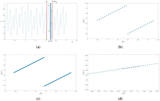
Figure 7. (a) Generating points are shown as green closed circles in the interval $[{\Phi }_1,{\Phi }_1+L_G]$. The number of generating points is not sufficient to cover the whole interval $[{\Phi }_1,{\Phi }_1+L_G]$ by subintervals $[{\varphi }_0^l(M_1\left(n\right),n),{\varphi }_0^r(M_1\left(n\right),n)]$ of the width $2\delta$ as the interval $\Delta =2\delta$ shown as a blue strip does not contain any generating point. The number of channels should be further increased to provide at least one generating point within the interval $\Delta$. (b,c) Distribution of generating points over the interval $[{\Phi }_1,{\Phi }_1+L_G]$: the position of the next generating point shown with respect to the previous generating point. The number of generating points P is (b) $P=500$ and (c) $P=5000$. (d) Distribution of generating points over the sub-interval $[2.1285,2.1307]$ randomly selected from the interval $[{\Phi }_1,{\Phi }_1+L_G]$. Distribution is not spatially uniform and contains clusters of points appearing at a finer spatial scale. The total number of the generating points is $P=5000$; cf. Figure 7c.

Conversely, increasing N when the channel width decreases will produce new generating points. Thus, the following question arises from the above consideration: given the number of generating points, where will the next generating point be placed over the interval $[{\Phi }_1,{\Phi }_1+L_G]$? In the following, we demonstrate that the position (26) of every next generating point cannot be predicted; that is, the generating points are randomly located in the interval $[{\Phi }_1,{\Phi }_1+L_G]$.

The randomness of generating points originates from the definition of the number $\pi$. We have $\pi =\lfloor \pi \rfloor +d_{\pi }$, where $d_{\pi }=0.14159265...\in (0,1)$. Let us present the fractional part $d_{\pi }$ as

$$d_{\pi }={\omega }_1{10}^{-1}+{\omega }_2{10}^{-2}+{\omega }_3{10}^{-3}+\dots =\sum _{p=1}^{\infty }{\omega }_p{10}^{-p}.$$

(30)

The decimal digits of the transcendental number $\pi$ can be determined using digit-extraction algorithms where the nth decimal digit can be computed without requiring the computation of earlier digits; e.g., see [33]. Meanwhile, various studies [34,35,36] have demonstrated that the sequence of decimal digits ${\omega }_1,{\omega }_2,{\omega }_3,\dots$ in (30) is random. In particular, it has been argued in [36] that the number $\pi$ can be used as a random number generator. Although randomness of the sequence ${\omega }_1,{\omega }_2,{\omega }_3,\dots$ remains an open question that discussion is far beyond the scope of this paper, once the randomness of the decimal digits of $\pi$ has been admitted it has far-reaching consequences in our problem. Consider $n\pi =n(\lfloor \pi \rfloor +d_{\pi })=n\lfloor \pi \rfloor +n{d}_{\pi },$ for an arbitrary $n\in \mathbb{N}$. Using expansion (30) gives

$$n{d}_{\pi }=A+\sum _{p=1}^{\infty }{\tilde{\omega }}_p{10}^{-p},$$

where $A\ge 0$ is an integer number, and the new expansion coefficients ${\tilde{\omega }}_p$ have been obtained by multiplying and adding terms in a random sequence $\{{\omega }_1,{\omega }_2,{\omega }_3,\dots \}$. Hence, the number $n\pi$ is

$$n\pi =\lfloor n\pi \rfloor +d_{n\pi },$$

(31)

where $d_{n\pi }\in (0,1)$ and a sequence of decimal digits in the fractional part $d_{n\pi }$ is random.

Let now ${\varphi }_i^G$, $i=2,3\dots$, be a new generating point added to the system. The point ${\varphi }_i^G$ is defined by (26) for some $n\in \mathbb{N}$ and $\alpha \left(n\right)\in [0,L_G]$. On the other hand, we have $m\left(n\right)=M_1\left(n\right)$ in (11) when ${\varphi }_0^l={\varphi }_i^G$ and direct computation results in

$${\varphi }_i^G=n\pi -\delta -M_1\left(n\right)=(n-1)\pi +\pi -\delta -\lceil (n-1)\pi \rceil =\pi -\delta -1+(n-1)\pi -\lfloor (n-1)\pi \rfloor .$$

(32)

Comparison of (26) and (32) gives $\alpha \left(n\right)=(n-1)\pi -\lfloor (n-1)\pi \rfloor =d_{(n-1)\pi }$. Hence, the generating point is

$${\varphi }_i^G=\pi -\delta -1+d_{(n-1)\pi },$$

(33)

where $0<d_{(n-1)\pi }\le L_G$. Since a sequence of decimal digits in the fractional part $d_{(n-1)\pi }$ of the number $(n-1)\pi$ is random, the position of the next generating point ${\varphi }_i^G$ appearing in the interval $[{\Phi }_1,{\Phi }_1+L_G]$ cannot be predicted as the number of channels increases. In other words, the grids $G_i$ produced by the points ${\varphi }_i^G$, $i=1,2,3\dots$ are randomly shifted with respect to each other.

The distribution of generating points over the interval $[{\Phi }_1,{\Phi }_1+L_G]$ is illustrated in Figure 7b–d, where we show the position of the next generating point with respect to the previous generating point. The number of generating points P increases from $P=500$ in Figure 7b to $P=5000$ in Figure 7c, confirming that the generating points tend to be distributed over the entire interval $[{\Phi }_1,{\Phi }_1+L_G]$. However, their distribution is not uniform as strong clustering of generating points occurs at a finer spatial scale (see Figure 7d) where the appearance of any new cluster of points cannot be predicted.

Consider any point ${\varphi }_0^{\ast }\in [{\varphi }_0^l(m^{\ast },n),{\varphi }_0^r(m^{\ast },n)]$ for which the exit time is $t_e=m^{\ast }$. Let ${\varphi }_0^{\ast }$ belong to the grid $G_i$ defined by a generating point ${\varphi }_i^G$. Let us now give a perturbation of the size $2\delta$ to the initial condition ${\varphi }_0^{\ast }$, where we assume that $\delta$ is small enough, i.e., $2\delta <L_G$. Since the new point ${\varphi }_0^{\ast \ast }={\varphi }_0^{\ast }+2\delta$ is outside the interval $({\varphi }_0^l(m^{\ast },n),{\varphi }_0^r(m^{\ast },n))$, the particle initially located at ${\varphi }_0^{\ast \ast }$ will have a different exit time $t_e=m^{\ast \ast }$. Furthermore, the point ${\varphi }_0^{\ast \ast }$ does not belong to the same grid $G_i$ to which the point ${\varphi }_0^{\ast }$ belongs because the distance between them is less than $L_G$ (see the discussion in Section 4).

Let us assume that ${\varphi }_0^{\ast \ast }\in G_j$, $j\ne i$. Since the grids $G_i$ and $G_j$ are randomly shifted with respect to each other, the difference $\Delta t_e=m^{\ast \ast }-m^{\ast }$ between the exit times when the particle is initially positioned at the point ${\varphi }_0^{\ast }$ or at the point ${\varphi }_0^{\ast \ast }$ cannot be determined a priori. Hence, any perturbation of the size $2\delta$ in the initial condition results in an unpredictable change in exit time. For the channel half-width $\delta \to 0$, the system goes to the state we refer to as countable chaos in Section 7 below.

The increasing unpredictability of the system as the channel becomes more narrow is shown in Figure 8, where the channel half-width decreases from $\delta =0.1$ in Figure 8a to $\delta =0.005$ in Figure 8d. We want to emphasise here that although a visual inspection of the graphs in Figure 8 may suggest their periodicity, those graphs are not periodic (see also the discussion in Section 8). The positions of local minima and maxima in each graph in the figure are not equidistant along the ${\varphi }_0$-axis: they are slightly yet randomly shifted from an equidistant distribution where a random shift of the maxima and minima points in the graph is a consequence of a random distribution of generating points over the interval $[{\Phi }_1,{\Phi }_1+L_G]$; cf. Figure 7b–d.

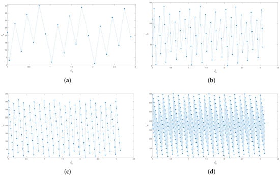
Figure 8. The graph $t_e\left({\varphi }_0^l(m,n)\right)$ for various channel half-width $\delta$ when the number of channels is $N=N_{min}$. The left boundaries ${\varphi }_0^l(m,n)$ of intervals $[{\varphi }_0^l(m,n),{\varphi }_0^r(m,n)]$ where the exit time remains constant are shown as blue closed circles in the graph. The number $N_{min}$ increases as the channel width decreases resulting in stronger unpredictability in the exit time $t_e$ as indicated by the increasing number of jumps $N_J$ and the increasing maximum jump amplitude $J_{max}$ in the system. (a) The channel half-width is $\delta =0.1$, the number of channels is $N_{min}=7$, the number of jumps is $N_J=21$, the maximum jump is $J_{max}=25$ (b) $\delta =0.05$, $N_{min}=26$, $N_J=80$, $J_{max}=113$ (c) $\delta =0.01$, $N_{min}=61$, $N_J=188$, $J_{max}=333$ (d) $\delta =0.005$, $N_{min}=114$, $N_J=354$, $J_{max}=377$.

It can be seen from Figure 8 that oscillations in the exit time shown in the $t_e\left({\varphi }_0^l(m,n)\right)$-plane become more severe as $\delta$ decreases. The analysis of the graphs in the figure also reveals that the maximum exit time increases as the channel narrows. Thus, our next aim is to investigate what conclusions can be drawn about the exit time $t_e$ in the extreme case of an infinitely narrow channel $\delta \to 0$.

7. Countable Chaos

In this section, we check to what extent the exit time is sensitive to initial conditions in the system with an infinitely narrow channel. Sensitivity to initial conditions is a pivotal feature of chaos, and investigating this issue should help us to decide whether the system (1)–(2) has chaotic properties when the channel width becomes infinitely small. The sensitivity to initial conditions can be confirmed by calculating Lyapunov exponents, where a dynamical system that has at least one positive Lyapunov exponent is considered chaotic [20,21,22]. However, the maximal Lyapunov exponent calculated for a simple linear map (2a) is $\lambda =0$. Therefore, we suggest an alternative approach to measure the divergence of the nearby trajectories as the channel half-width $\delta \to 0$.

Consider the total escape defined by the number of channels $N_{min}$ for the given channel width $\delta$ and let $P=P\left(\delta \right)$ be the number of subintervals where the exit time $t_e$ remains constant. The number of jumps $N_J$ between those subintervals is given by

$$N_J=P-1.$$

(34)

Let us numerate the subintervals of constant exit time with the index $p=1,2,\dots ,P$. The jump magnitude $J_p$ is then defined for each jump between the subintervals as

$$J_p=\mid t_e\left({\varphi }_0^l(p+1)\right)-t_e\left({\varphi }_0^l\left(p\right)\right)\mid ,p=1,2,\dots ,N_J,$$

(35)

where ${\varphi }_0^l\left(p\right)$ is the left boundary of the p-th sub-interval $[{\varphi }_0^l\left(p\right),{\varphi }_0^r\left(p\right)]$.

Consider two trajectories starting at points ${\varphi }_0^I$ and ${\varphi }_0^{II}$ separated by the distance $ϵ$ in the domain $[0,{\varphi }_{max})$, where we assume that ${\varphi }_0^{II}={\varphi }_0^I+ϵ$ for the sake of convenience. Let ${\varphi }_0^l\left(p\right)<{\varphi }_0^I<{\varphi }_0^r\left(p\right)$ and ${\varphi }_0^l(p+1)<{\varphi }_0^{II}<{\varphi }_0^r(p+1)$; i.e., there is a jump $J_p$ located within the interval $[{\varphi }_0^I,{\varphi }_0^{II}]$. Let also $t_e\left({\varphi }_0^l(p+1)\right)>t_e\left({\varphi }_0^l\left(p\right)\right)$, and then the length $l_1\left(t\right)$ of the first trajectory remains the same for any time $t>t_e\left({\varphi }_0^l\left(p\right)\right)$ as the particle has already left the domain. It follows from (2) that the distance between the two trajectories accumulated over time $t\in [t_e\left({\varphi }_0^l\left(p\right)\right),t_e\left({\varphi }_0^l(p+1)\right)]$ is $d\left(t\right)={\varphi }_0^{II}+t-l_1\left(t_e\right)>0$ for $\Delta \varphi =1$. Substituting ${\varphi }_0^{II}={\varphi }_0^I+ϵ$ and $l_1\left(t_e\right)={\varphi }_0^I+t_e\left({\varphi }_0^l\left(p\right)\right)$ into the above expression, we obtain

$$d\left(t\right)=t-t_e\left({\varphi }_0^l\left(p\right)\right)+ϵ,$$

(36)

i.e., the distance $d\left(t\right)$ between the trajectories grows linearly with time. The maximum distance between the trajectories is $d_{max}=d\left(t_e\left({\varphi }_0^l(p+1)\right)\right)=t_e\left({\varphi }_0^l(p+1)\right)-t_e\left({\varphi }_0^l\left(p\right)\right)+ϵ$= $\mid t_e(\left({\varphi }_0^l(p+1)\right)-t_e\left({\varphi }_0^l\left(p\right)\right)\mid +ϵ=J_p+ϵ$ and we have

$$d_{max}\to J_{p}asϵ\to 0,$$

(37)

where the jump magnitude $J_p$ remains unknown until the solution $t_e\left({\varphi }_0\right)$ is obtained in the entire domain of definition $[0,{\varphi }_{max})$.

Given the results (36) and (37), we note that separation of trajectories (36) occurs over a finite time only. In addition, many trajectories that have the distance $ϵ$ between them at time $t=0$ will have the same distance $ϵ$ between them at any time $t>0$. Since the function $t_e\left({\varphi }_0\right)$ is piecewise constant, the size of the subdomain of the initial condition where trajectories that are initially a very small distance apart will diverge over time depends on the number of jumps and can be evaluated as $2ϵN_J$. Consider, for example, $\delta =0.1$ (see the baseline case in Section 3) and $ϵ=0.005$. We have the number of jumps $N_J=21$, as seen in Figure 6, which results in $2ϵN_J=0.21$, while the total size of the domain $[0,{\varphi }_{max})$ where the trajectories start is ${\varphi }_{max}=\pi -\delta \approx 3.0416$.

Meanwhile, it has been proved in Section 3 that the maximum length of each subinterval $[{\varphi }_0^l\left(p\right),{\varphi }_0^r\left(p\right)]$ where the exit time $t_e$ remains constant is $2\delta$. Hence, for any given $ϵ>0$ there exists a channel half-width ${\delta }^{\ast }={\delta }^{\ast }\left(ϵ\right)$ such that any two trajectories initially separated by the distance $ϵ$ will have a different exit time for any $\delta <{\delta }^{\ast }$, no matter where the interval $[{\varphi }_0^I,{\varphi }_0^{II}]$ is located within the domain $[0,{\varphi }_{max})$.

The threshold value ${\delta }^{\ast }$ can be chosen as ${\delta }^{\ast }=ϵ/2$ and any two trajectories that are initially a distance $ϵ$ apart will then be separated as (36) in the system with a channel half-width $\delta <{\delta }^{\ast }$. The above conclusion also implies that the number of jumps (34) depends on the parameter $\delta$, and $N_J\left(\delta \right)$ increases as $\delta$ decreases. For $ϵ=0.005$ in the above example, we require ${\delta }^{\ast }=0.0025$ to provide further separation of all trajectories separated initially by $ϵ$ and the number of jumps increases from $N_J=21$ to $N_J=23,281$ when the channel half-width decreases from $\delta =0.1$ to ${\delta }^{\ast }=0.0025$.

Let us demonstrate that the separation of trajectories becomes stronger in the entire domain $[0,{\varphi }_{max})$ as the channel half-width $\delta$ decreases. Since the solution to the problem (2)–(4) is available for any $\delta >0$, we find the maximum distance between the trajectories (37) in the whole domain of the initial condition $[0,{\varphi }_{max})$ by direct computation of the jumps (35) in the function $t_e\left({\varphi }_0\right)$. For any given channel half-width $\delta$, we introduce the maximum jump $J_{max}$,

$$J_{max}=\underset{p}{max}(J_1,J_2,\dots ,J_{N_J}).$$

(38)

The maximum jump $J_{max}$ depends on $\delta$, because it follows from the analysis in Section 3 and Section 5 that the maximum exit time $t_e^{max}$ can be evaluated as

$$t_e^{max}>{\displaystyle \frac{\pi -\delta }{2\delta }},$$

(39)

for the given channel half-width $\delta$. We then conclude from (39) that

$$J_{max}\left(\delta \right)\to \infty as\delta \to 0.$$

(40)

We also compute the average jump $J_{av}$ in the domain $[0,{\varphi }_{max})$,

$$J_{av}={\displaystyle \frac{1}{N_J}}\sum _{p=1}^{N_J}{J}_p.$$

(41)

The average jump $J_{av}$ depends on $\delta$, since the number of jumps $N_J$ defined by (34) increases when the channel half-width $\delta$ decreases; see the discussion in Section 6.

The increase in the number of jumps $N_J$ as $\delta$ decreases is illustrated by Figure 8, where we also provide the value of $J_{max}$ in the caption of the figure for each $\delta$ considered in the figure. We then show the graphs $J_{max}\left(\delta \right)$ and $J_{av}\left(\delta \right)$ on a logarithmic scale in Figure 9a, where the channel half-width varies from $\delta ={10}^{-1}$ to $\delta ={10}^{-3}$. It can be readily noticed from the figure that the maximum distance between the trajectories $J_{max}$ (38) and the average distance between the trajectories $J_{av}$ (41) increase when the parameter $\delta$ decreases.

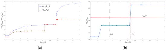
Figure 9. (a) The maximum jump $J_{max}$ (38) (blue solid line, blue stars) and the average jump $J_{av}$ (41) (red dashed line, red closed circles) as functions of the channel half-width $\delta$. The graphs $J_{max}\left(\delta \right)$ and $J_{av}\left(\delta \right)$ are shown on a logarithmic scale. The distance between trajectories measured by (38) and (41) increases as the channel half-width decreases. (b) The minimum jump $J_{min}$ (42) (blue solid line, blue closed circles) is computed for the same range of the channel half-width $\delta$ as the graphs in Figure 9a. Since $J_{min}$ increases as $\delta$ decreases, it is possible to find $\delta ={\delta }^{\ast \ast }$ for which the final distance $d_{max}$ between nearby trajectories will be $d_{max}>J$ (see further explanation in the text).

An important observation about the graphs in Figure 9a is that intervals of very rapid growth are interspersed with intervals where the functions (38) and (41) remain constant. A slight change in the parameter $\delta$ does not necessarily result in an increase in the number of channels required for the total escape. For example, the number of jumps is $N_J=21$ for $\delta =0.1$ in Figure 6b. If we decrease the channel half-width from $\delta =0.1$ to $\delta =0.09$, the position of each jump in the exit time $t_e\left({\varphi }_0\right)$ in Figure 6b will change, but the number of channels required for the total escape will remain $N_{min}=7$. Consequently, we will have the same number of jumps $N_J=21$ and the same maximum jump amplitude $J_{max}=25$ as the graphs in Figure 9a show.

We now define the minimum jump $J_{min}$ in the domain $[0,{\varphi }_{max})$,

$$J_{min}=\underset{p}{min}(J_1,J_2,\dots ,J_{N_J}).$$

(42)

If the minimum jump is a monotone function of $\delta$ and we have

$$J_{min}\left(\delta \right)\to \infty as\delta \to 0,$$

(43)

then sensitive dependence on initial conditions can be defined in the system when $\delta \to 0$. Consider an arbitrary distance $J>0$. Under the above assumptions about $J_{min}\left(\delta \right)$, for any two trajectories initially separated by the distance $ϵ$ there exists the channel half-width $\delta ={\delta }^{\ast \ast }<{\delta }^{\ast }=ϵ/2$ such that the final distance (37) between these trajectories will be $d_{max}>J$. We note that the channel half-width ${\delta }^{\ast \ast }$ can be found from condition $J_{min}\left({\delta }^{\ast \ast }\right)=J$.

The graph $J_{min}\left(\delta \right)$ is shown on a logarithmic scale in Figure 9b for the same values of the parameter $\delta$ as the graphs in Figure 9a. Given $ϵ>0$, consider an arbitrary distance $J>0$ (solid red line in the figure). For any channel half-width $\delta <{\delta }^{\ast }$ (vertical black dashed line), any two trajectories separated initially by the distance $ϵ$ will have the distance $d_{max}>ϵ$ between them, but the condition $d_{max}>J$ will not be held for all such trajectories. Consider now $\delta ={\delta }^{\ast \ast }$ (vertical red dashed line). For any $\delta <{\delta }^{\ast \ast }$, the distance $d_{max}$ (37) between any two trajectories initially separated by the distance $ϵ$ is $d_{max}>J$.

Let us note that we have only used the term ‘chaos’ in this section to indicate the sensitivity to initial conditions in the problem as $\delta \to 0$. Furthermore, the definition of sensitive dependence above is different from the conventional definition of sensitive dependence on initial conditions (see e.g., [37,38]) since it is based essentially on the asymptotic behaviour of the system when $\delta \to 0$. The sensitivity to initial conditions in the problem manifests itself through an infinitely large number of singular points (jumps) $N_J$ in the function $t_e\left({\varphi }_0\right)$ whose locations cannot be predicted a priori. We have $N_J\to \infty$ as $\delta \to 0$ because the exit time $t_e$ is different for any two points initially separated by the distance $ϵ>2\delta$ in the domain $[0,{\varphi }_{max})$. As the number of jumps increases, so does their magnitude. The maximum jump (38) in the entire domain of the initial condition $[0,{\varphi }_{max})$ is $J_{max}\to \infty$ as $\delta \to 0$. The numerical results of Figure 9b suggest that the minimum jump $J_{min}$ (42) in the domain $[0,{\varphi }_{max})$ is $J_{min}\to \infty$ as $\delta \to 0$, although we do not provide a rigorous mathematical proof of this statement. Since the maximum distance $d_{max}$ between the two trajectories is measured by the jump magnitude (37), any two trajectories initially separated by given $ϵ>0$ will be separated by an arbitrarily large distance J in the system with an infinitely narrow channel $\delta \to 0$ under assumption (43).

Meanwhile, one can say that for any finite channel half-width $\delta >0$, there is no chaos in the system. The number of random jumps in the function $t_e\left({\varphi }_0\right)$ is finite for any finite $\delta$ and there are a number of subintervals where the exit time remains constant. The number of jumps increases as the channel width decreases, yet the exit time can be accurately calculated by Algorithm 1 for any given $\delta >0$ and any ${\varphi }_0\in [0,{\varphi }_{max})$ to remove unpredictability. Since the function $t_e\left({\varphi }_0\right)$ is entirely defined by generating points belonging to a countable set, a finite number of intervals $[{\varphi }_0^l,{\varphi }_0^r]$ are required to fill any gap along the ${\varphi }_0$-axis and therefore determine the exit time $t_e$ for any ${\varphi }_0$ taken from the domain of definition. Hence, we also introduce the term ‘countable’ to emphasise the discrete nature of the process, as all exit times belong to a countable set and can be computed, no matter how small a finite channel half-width $\delta$ is.

8. Discussion and Conclusions

We have studied a linear dynamical system resulting from discrete time motion of a particle along a unit circle that has an escape channel of width $2\delta$. The time $t_e$ required for the particle to approach the escape channel and exit the circle through it depends on the initial position of the particle ${\varphi }_0$ and it has been argued in the paper that the solution $t_e\left({\varphi }_0\right)$ is ‘global’; that is, finding the exit time for any given ${\varphi }_0$ requires reconstruction of the function $t_e\left({\varphi }_0\right)$ in the entire domain of definition ${\varphi }_0\in [0,{\varphi }_{max})$. The function $t_e\left({\varphi }_0\right)$ is piecewise constant and the exit time remains the same at subintervals of length $2\delta$ at most and has jumps between those subintervals. Hence, given the channel half-width $\delta$, a slight change in the initial condition ${\varphi }_0$ can leave the exit time the same or result in a significant change in the exit time. The system’s response to a slight change in the initial condition cannot be predicted unless the function $t_e\left({\varphi }_0\right)$ is computed everywhere in the domain ${\varphi }_0\in [0,{\varphi }_{max})$.

The dynamical system (1)–(2) studied in the paper presents a convenient formulation of a blind search in confined space problem where the results of our study allow one to conclude about the completeness and time complexity criteria of the search. Completeness of the search follows from randomness of generating points (see Section 4 and Section 6) since that property implies covering the whole interval $[{\Phi }_1,{\Phi }_1+L_G]$ by subintervals $[{\varphi }_0^l(M_1\left(n\right),n),{\varphi }_0^r(M_1\left(n\right),n)]$ with no gaps between them as required to find the exit time for any given initial position of the particle. It also follows from the above requirement that the solution is ${\displaystyle t_e\left({\varphi }_0\right)\sim \frac{1}{\delta }}$ when the question of time complexity is addressed.

One important result of our study is that the number of random jumps in the function $t_e\left({\varphi }_0\right)$ becomes infinitely large resulting in arbitrary separation of nearby trajectories as the channel half-width $\delta \to 0$: the phenomenon of countable chaos arises in the problem with an infinitely narrow channel. The countable chaos is not a conventional chaos definition because it only reveals itself as $\delta \to 0$ and also because the system has noise that induces sensitive dependence on initial conditions (cf. [12] where it was argued that the system is not chaotic if there is external noise responsible for irregularity in the behaviour of the system). However, the noise is not external and is inherent in the system. The number $\pi$ responsible for the definition of circular motion also acts as a random number generator which produces sensitivity to initial conditions when the channel half-width $\delta \to 0$.

The unpredictability of the exit time observed in the system for any finite channel half-width $\delta$ and the requirement to obtain a global solution $t_e\left({\varphi }_0\right)$, ${\varphi }_0\in [0,{\varphi }_{max})$ to find the exit time $t_e$ for a given initial position of the particle may be considered undesirable features of the system as they increase the time complexity in the blind search problem. However, the presence of inherent noise actually makes the blind search more successful because it increases the probability of escape. Removing the noise in the problem will result in the ‘the escape is/is not ever possible’ dichotomy as illustrated by the following example.

Let us make the system fully predictable by turning off the random number generator. That is, we want to consider a hypothetical system in which the first channel is located at $\tilde{\pi }=3.14$ and the distance between channels is $2\tilde{\pi }=6.28$. This hypothetical $‘\tilde{\pi }$-system’ can be thought of as a setup where circular motion is replaced by linear motion; i.e., a unit circle is approximated by a polygon.

Generating points in the new $\tilde{\pi }$-system are periodic as the equation

$$i{L}_G=j\Delta \varphi ,$$

(44)

has a solution $(i,j)\in \mathbb{N}$. For $\Delta \varphi =1$ and the generating length $L_G=2\tilde{\pi }-\lfloor 2\tilde{\pi }\rfloor$, we find $i=25$ and $j=7$. In other words, the residual $i{L}_G$ accumulated during the discrete time motion over the domain with $i=25$ channels (see Section 3) can be fully covered in the $j=7$ additional steps of the particle. It is also obvious that Equation (44) does not have any solution $(i,j)\in \mathbb{N}$ when $L_G=2\pi -\lfloor 2\pi \rfloor$ in the original $‘\pi$-system’ because $\pi$ is not a rational number.

We want to find the number of channels $N_{min}$ required to make the total escape $P_e=1$ as explained in Section 5. Let us first consider the baseline case $\delta =0.1$, $\Delta \varphi =1$ in the original $\pi$-system where the particle moves along a circle. We have $P_e=1$ for $N_{min}=7$ channels; see Figure 6b. Direct computation reveals that linear motion in the new $\tilde{\pi }$-system results in the same number of channels required for the total escape; i.e., we have $N_{min}=7$.

We now decrease the channel half-width as $\delta =0.01$. For circular motion (the $\pi$-system), the total escape $P_e$ will be achieved when there are $N_{min}=61$ channels in the system. However, the results are very different when linear motion (the $\tilde{\pi }$-system) is considered. The escape range $P_e=0.4984\approx 0.5$ is established over the first $N=25$ channels and then $P_e$ does not change as $N\to \infty$ due to the periodicity of the generating points. If we have an ensemble of particles statistically uniformly distributed throughout the interval ${\varphi }_0\in [0,{\varphi }_{max})$ at time $t=0$, approximately half of them will escape from the domain, while another half will stay in the domain forever. Hence, the fully predictable $\tilde{\pi }$-system can also be thought of as a half-degenerate system because the goal state is never achieved by approximately $50\%$ of the population.

In the case of circular motion, all particles will sooner or later exit the domain, no matter how narrow the escape channel is. The definition of $\pi$ makes the system’s behaviour less predictable and more complex, yet the system is not degenerate. The complexity induced by $\pi$ should be taken into account when tracing the trajectories, but that complexity is an advantage rather than a drawback because it removes the escape dichotomy in the system.

In conclusion, we note that we have been concerned in this paper with reporting random exit times for any finite channel half-width $\delta$ and sensitivity to initial conditions in the system (1) and (2) as $\delta \to 0$ rather than investigating those phenomena in detail. Thus, our study leaves a number of open questions, some of them listed below.

Chaotic properties of the system: The divergence of nearby trajectories has been demonstrated in Section 7, yet more thorough investigation of the condition (43) is necessary to draw a rigorous conclusion about sensitive dependence on initial conditions in the system with an infinitely narrow channel. Furthermore, our study has been focused on sensitivity to initial conditions only as we have assumed that this is the most important property defining a chaotic system in line with the Experimentalists’ definition in [11]. Although there is no universally accepted definition of chaos in a dynamical system so far [19], other definitions of chaos provided, e.g., in [13] or [17], require additional properties of a dynamical system to conclude that the system is chaotic. Those properties will be verified in future work on the problem to see whether the definition of a chaotic regime in the system (1) and (2) can be made compatible with widely accepted definitions of chaos.

Weak chaos: It has been shown in Section 7 that the separation of trajectories occurs weaker than exponentially as the distance between them increases linearly over time. The slower separation of chaotic trajectories is a feature of weak chaos reported, e.g., in [29,30,31,39], and comparison of the system’s asymptotical behaviour as $\delta \to 0$ with systems where weak chaos has been detected is reserved as a topic of future work. Also, it is still unclear how quickly trajectories diverge on average when the parameter $\delta$ decreases. A related question that arises here is whether the transition between domains where the functions $J_{min}\left(\delta \right)$ and $J_{max}\left(\delta \right)$ remain constant is continuous (albeit with a very steep gradient) or discontinuous in Figure 9. The latter case may be related to the appearance of new generating points in the system when $\delta$ decreases, and this issue requires further investigation because it may help us evaluate how fast the system moves to a chaotic regime as $\delta \to 0$.

System parameters: The analysis in the paper has been made for the step size of the particle $\Delta \varphi =1$. If a different step size $\Delta \varphi$ is considered under the condition $\Delta \varphi >2\delta$, then Algorithm 1 in Section 5 can be used to find the exit time for any finite channel half-width $\delta$. The conclusions made about sensitive dependence on initial conditions in Section 7 will also remain the same if a different (yet finite) value $\Delta \varphi$ is chosen in the problem. Meanwhile, the asymptotic behaviour of the system when $\delta \to 0$ and $\Delta \varphi \to 0$ is unclear and should be studied in future work.

Pseudo-random number generators: The randomness of the decimal digits of $\pi$ has been the most important assumption made in the paper. The ability of irrational numbers to serve as pseudo-random number generators has been the focus of research for many years [40], yet this topic remains a big and challenging problem. If we have a rigorous confirmation on the randomness of an irrational number p, an algorithm similar to that presented in the paper can be designed for the number p when a particle performs discrete time motion (1) and (2) along a closed curve of length $\left|p\right|$. On the other hand, if the number p does not have a random sequence of decimal digits, then using it in the problem will result in different properties of the dynamical system (1) and (2). Generating points will not be located randomly and that, in turn, will result in only a limited number of trajectories escaping from the domain (cf. the conclusions for the rational number $\tilde{\pi }$ in this section). Thus, we hope that the results of this paper may spark new interest in research on pseudo-random number generators.

Meanwhile, the solution algorithm in Section 5 allows one to study more complex problems based on the results already obtained in this paper. The idealistic setting (1)–(2) employed in the problem can serve as an approximation to various realistic problems, including those in scattering theory [41], animal foraging in a spatial domain [8], cryptography [42], and detection of pulsed signals [43]. If the problem is considered in the framework of classical scattering, one question of interest could be to move from consideration of a single particle to an ensemble of particles. For instance, the approach developed in this paper allows for finding the probability of the event that all particles will leave the domain over a given time, the answer to the above question depending on the initial spatial distribution of particles. In addition, the channel width can be varied with time in order to maximise or minimise the exit time over which all particles will leave the domain.

Alternatively, the blind search problem can be thought of as a foraging problem in which an animal is looking for a profitable patch $[\pi -\delta ,\pi +\delta ]$. In the latter case, the setup (1)–(2) with a single animal can be further investigated if the condition of having a constant step size is relaxed. Although the requirement of discrete time is essential in animal movement models, more realistic movement rules will involve consideration of a stochastic step length defined by a Lévy walk or flight [44]. Furthermore, even when the movement is not random, the step length $\Delta \varphi$ is likely to vary as the animal tries to optimise the search time. This brings the system to a new level of complexity, and the study of a variable step length is considered a topic of future work.

References

- Russell, S.; Norvig, P. Artificial Intelligence: A Modern Approach; Pearson: London, UK, 2013. [Google Scholar]
- Bellman, R. On a routing problem. Q. Appl. Math. 1958, 16, 87–90. [Google Scholar] [CrossRef]
- Dijkstra, E.W. A note on two problems in connexion with graphs. Numer. Math. 1959, 1, 269–271. [Google Scholar] [CrossRef]
- Korf, R.E. Depth-first iterative-deepening: An optimal admissible tree search. Artif. Intell. 1985, 27, 97–109. [Google Scholar] [CrossRef]
- Meinshausen, N.; Bickel, P.; Rice, J. Efficient blind search: Optimal power of detection under computational cost constraints. Ann. Appl. Stat. 2009, 3, 38–60. [Google Scholar] [CrossRef]
- Silvela, J.; Portillo, J. Breadth-first search and its application to image processing problems. IEEE Trans. Image Process. 2001, 10, 1194–1199. [Google Scholar] [CrossRef]
- Liang, H.; Chen, Z.; Fang, G. A depth-first search algorithm for oligonucleotide design in gene assembly. Front Genet. 2022, 13, 1023092. [Google Scholar] [CrossRef]
- Kagan, E.; Ben-Gal, I. Search and Foraging: Individual Motion and Swarm Dynamics; CRC Press: Boca Raton, FL, USA, 2015. [Google Scholar]
- Humphries, N.E.; Sims, D.W. Optimal foraging strategies: Lévy walks balance searching and patch exploitation under a very broad range of conditions. J. Theor. Biol. 2014, 358, 179–193. [Google Scholar] [CrossRef]
- Hutchinson, J.M.; Stephens, D.W.; Bateson, M.; Couzin, I.; Dukas, R.; Giraldeau, L.A.; Hills, T.T.; Méry, F.; Winterhalder, B. Searching for fundamentals and commonalities of search. In Cognitive Search: Evolution, Algorithms, and the Brain; MIT Press: Davis, CA, USA, 2012. [Google Scholar]
- Martelli, M.; Dang, M.; Seph, T. Defining chaos. Math. Mag. 1998, 71, 112–122. [Google Scholar] [CrossRef]
- Strogatz, S.H. Nonlinear Dynamics and Chaos; Perseus Books Publishing: New York, NY, USA, 1994. [Google Scholar]
- Devaney, R.L. An Introduction to Chaotic Dynamical Systems; Addison-Wesley: Boston, MA, USA, 1989. [Google Scholar]
- Li, T.; Yorke, J.A. Period three implies chaos. Am. Math. Mon. 1975, 82, 985–992. [Google Scholar] [CrossRef]
- Martelli, M. Introduction to Discrete Dynamical Systems and Chaos; John Wiley & Sons, Inc.: Hoboken, NJ, USA, 1999. [Google Scholar]
- Shi, Y.; Chen, G. Chaos of time-varying discrete dynamical systems. J. Differ. Equ. Appl. 2009, 15, 429–449. [Google Scholar] [CrossRef]
- Wiggins, S. Chaotic Transport in Dynamical Systems. Interdisciplinary Applied Mathematics; Springer: Berlin/Heidelberg, Germany, 1992; Volume 2. [Google Scholar]
- Leiber, T. On the impact of deterministic chaos on modern science and the philosophy of science: Implications for the philosophy of technology? Soc. Philos. Technol. Q. Electron. J. 1998, 4, 93–110. [Google Scholar] [CrossRef]
- Sprott, J.C. Chaos and Time-Series Analysis; Oxford University Press: Oxford, UK, 2003. [Google Scholar]
- Benettin, G.; Galgani, L.; Giorgilli, A.; Strelcyn, J.M. Lyapunov characteristic exponents for smooth dynamical systems and for hamiltonian systems; A method for computing all of them. Part 1: Theory. Meccanica 1980, 15, 9–20. [Google Scholar] [CrossRef]
- Datseris, G.; Parlitz, U. Nonlinear Dynamics: A Concise Introduction Interlaced with Code; Springer Nature: Berlin/Heidelberg, Germany, 2022. [Google Scholar]
- Schuster, H.G.; Just, W. Deterministic Chaos: An Introduction; Wiley-VCH: Weinheim, Germany, 2005. [Google Scholar]
- Banerjee, M.; Ghosh, S.; Manfredi, P.; d’Onofrio, A. Spatio-temporal chaos and clustering induced by nonlocal information and vaccine hesitancy in the SIR epidemic model. Chaos Solitons Fractals 2023, 170, 113339. [Google Scholar] [CrossRef]
- Malchow, H.; Petrovskii, S.V.; Venturino, E. Spatiotemporal Patterns in Ecology and Epidemiology: Theory, Models, and Simulation; CRC Press: Boca Raton, FL, USA, 2007. [Google Scholar]
- Mokni, K.; Mouhsine, H.; Ch-Chaoui, M. Multi-parameter bifurcations in a discrete Ricker-type predator–prey model with prey immigration. Math. Comput. Simul. 2025, 233, 39–59. [Google Scholar] [CrossRef]
- Porcher, R.; Thomas, G. Estimating Lyapunov exponents in biomedical time series. Phys. Rev. E 2001, 64, 010902. [Google Scholar] [CrossRef]
- Vulpiani, A.; Cecconi, F.; Cencini, M. Chaos: From Simple Models to Complex Systems; World Scientific: Singapore, 2009. [Google Scholar]
- Wolf, A.; Swift, J.B.; Swinney, H.L.; Vastano, J.A. Determining Lyapunov exponents from a time series. Phys. D Nonlinear Phenom. 1985, 16, 285–317. [Google Scholar] [CrossRef]
- Klages, R. Microscopic Chaos, Fractals and Transport in Nonequilibrium Statistical Mechanics; World Scientific: Singapore, 2007. [Google Scholar]
- Nee, S. Survival and weak chaos. R. Soc. Open Sci. 2018, 5, 5172181. [Google Scholar]
- Ruiz, G.; Bountis, T.; Tsallis, C. Time-evolving statistics of chaotic orbits of conservative maps in the context of the central limit theorem. Int. J. Bifurc. Chaos 2012, 22, 1250208. [Google Scholar] [CrossRef]
- Petrovskii, S.V. (School of Computing and Mathematical Sciences, University of Leicester, Leicester, UK). The Blind Man Problem in a Unit Circle. Personal communication, 2020.
- Plouffe, S. A formula for the nth decimal digit or binary of π and πn. arXiv 2022, arXiv:2201.12601. [Google Scholar] [CrossRef]
- Bailey, D.H.; Borwein, J.M.; Calude, C.S.; Dinneen, M.J.; Dumitrescu, M.; Yee, A. An empirical approach to the normality of π. Exp. Math. 2012, 21, 375–384. [Google Scholar]
- Marsaglia, G. On the Randomness of π and Other Decimal Expansions. 2005. Available online: https://api.semanticscholar.org/CorpusID:45766422 (accessed on 1 February 2025).
- Tu, S.-J.; Fischbach, E. A study on the randomness of the digits of π. Int. J. Mod. Phys. C 2005, 16, 281–294. [Google Scholar]
- Alligood, K.T.; Sauer, T.S.; Yorke, J.A. Chaos—An Introduction to Dynamical Systems; Springer: Berlin/Heidelberg, Germany, 1997. [Google Scholar]
- Robinson, C. Dynamical Systems; CRC Press: Boca Raton, FL, USA, 1995. [Google Scholar]
- Zaslavskiî, G.M.; Sagdeev, R.Z.; Usikov, D.A.; Chernikov, A.A. Weak Chaos and Quasi-Regular Patterns; Cambridge University Press: Cambridge, UK, 1991. [Google Scholar]
- Bailey, D.H.; Crandall, R.E. Random generators and normal numbers. Exp. Math. 2002, 11, 527–546. [Google Scholar]
- Gaspard, P. Chaos, Scattering and Statistical Mechanics; Cambridge University Press: Cambridge, UK, 1998. [Google Scholar]
- Zhou, Y.; Bao, L.; Chen, C.P. A new 1D chaotic system for image encryption. Signal Process. 2014, 97, 172–182. [Google Scholar]
- Levanon, N.; Mozeson, E. Radar Signals; John Wiley & Sons, Inc.: Hoboken, NJ, USA, 2004. [Google Scholar]
- Viswanathan, G.M.; da Luz, M.G.E.; Raposo, E.P.; Stanley, H.E. The Physics of Foraging. An Introduction to Random Searches and Biological Encounters; Cambridge University Press: Cambridge, UK, 2011. [Google Scholar]
Disclaimer/Publisher’s Note: The statements, opinions and data contained in all publications are solely those of the individual author(s) and contributor(s) and not of MDPI and/or the editor(s). MDPI and/or the editor(s) disclaim responsibility for any injury to people or property resulting from any ideas, methods, instructions or products referred to in the content. |
© 2025 by the author. Licensee MDPI, Basel, Switzerland. This article is an open access article distributed under the terms and conditions of the Creative Commons Attribution (CC BY) license (https://creativecommons.org/licenses/by/4.0/).