Abstract
Onboard millimeter-wave radar is one way to improve helicopter flight safety at low altitudes in difficult meteorological conditions. Low-altitude flight is associated with the risk of collision with low-visibility obstacles such as power lines. Since power lines have the property of polarization anisotropy, it is necessary to use radar polarimetry methods to increase the radar visibility of such obstacles for detection. This paper investigates the possibility of identifying low-visibility polarization-anisotropic objects, such as power lines, in polarimetric images obtained by onboard helicopter radars to warn the pilot about the danger of a collision with a low-visibility object. Consequently, the use of a polarimetric radar with a polarization modulation of the emitted signal, the two-channel polarization synchronous reception of reflected signals and Eigenvalue signal processing in real time was proposed, aiming to eliminate the dependence of reflected signals on the spatial orientation of power transmission line wires. Additionally, an optimal algorithm for adaptive polarization selection, obtained by the maximum likelihood method, was proposed to detect such objects against the background of the underlying surface. The effectiveness of the proposed algorithm was tested using computer modeling methods. Moreover, a W-band polarimetric radar system was designed for experimental studies of this concept. The developed radar system provides digital real-time signal processing and the reconstruction of composite polarimetric images. It displays information about the polarization characteristics of the objects in the scanned area and the results of their polarization selection. Therefore, the system informs the pilot about dangerous objects along the helicopter’s route. Radar experimental tests in actual environmental conditions have confirmed the proposed concept’s correctness and the proposed method and algorithm’s effectiveness.
Keywords:
image registration; image processing; polarimetric image; polarimetric radar; eigenvalue signal processing; adaptive polarization selection MSC:
60G35; 68U10
1. Introduction
Helicopters are indispensable due to their mobility in approaching hard-to-reach places. They are widely used in firefighting, search and rescue operations, police and military operations, agriculture and construction, and medical transport [1]. Most helicopter operations are carried out at low altitudes, which creates risks of collision with various obstacles, especially in conditions of limited visibility, such as fog, rain and snow. Statistics on aviation accidents worldwide show that the largest share of accidents and disasters occur precisely during flights at low altitudes and during landing [2]. The highest level of danger in low-altitude flights, especially in mountainous areas [3], is represented by objects such as poles, towers, wires and power transmission line support [4,5].
To ensure the safety of helicopter flights at low altitudes, active [6] and passive optical systems [7,8], as well as infrared [9] ranges, are employed, including artificial intelligence methods [10]. However, the efficiency of such systems is significantly reduced in adverse weather conditions [11]. Therefore, systems operating in the radio range are considered the most promising for detecting low-visibility objects [12,13,14]. The radar cross-section (RCS) of narrow objects, such as power lines, is small compared to the powerful reflections from the underlying surface. Therefore, to detect them, it is necessary to increase the radar resolution, for example, using aperture synthesis methods [15,16]. However, the dependence of the signal power reflected by power lines on the polarization of the emitted signal requires the use of polarization methods for their detection.
Quite interesting results were obtained by S. Futatsumori and N. Miyazaki [17,18,19,20] using circularly polarized radars at 77 GHz and 94 GHz, which demonstrate the potential of employing polarimetric radars to detect power transmission lines. The polarization anisotropy of weak signals reflected by power lines allows the use of polarization selection methods to improve the signal-to-noise ratio (SNR) [21,22]. In [23], an algorithm for signal processing was developed for the polarization selection of small-sized polarization-anisotropic objects against the background of the Earth’s surface. This algorithm uses signals from two orthogonally polarized channels to receive radar signals. At the same time, some studies [24] have shown that using a fully polarized radar is the optimal way to detect low-visibility objects. Moreover, eigenvalue signal processing [25] is considered a solution to the polarization selection of polarization-anisotropic objects given an observation’s random angle. Therefore, it is widely employed in radar meteorology [26].
Most of the existing methods for detecting power transmission lines rely on circularly polarized signals [17,18,19,20] and dual-polarized channel processing [23]. We propose a novel eigenvalue-based method for polarization selection. Traditional techniques are limited by specific observation conditions and SNR improvements [21,22]. However, our method, unlike those approaches, uses full-polarization radar data [24] and eigenvalue processing to robustly separate polarization-anisotropic objects, such as power lines, from a background surface. This approach is particularly effective for detecting low-RCS objects at random observation angles, offering a significant advantage over existing solutions.
This work aims to study the possibility of identifying low-visibility polarization-anisotropic objects, such as power transmission lines, poles and towers, on polarimetric images obtained by onboard helicopter radars to warn the pilot about the danger of collisions with these objects.
The following tasks are accomplished in this work:
- Increasing the efficiency of polarization-anisotropic object detection by combining polarization selection methods with eigenvalue signal processing;
- Testing the performance of the developed methods and algorithms by computer simulation modeling and during physical experiments in real environmental conditions.
The rest of this paper is organized as follows: Section 2 presents the theoretical prerequisites for applying the polarization characteristics of various objects, the designed method for the polarization selection of polarization-anisotropic objects and the proposed processing block diagram with algorithmic operations. Section 3 presents simulation modeling results, confirming the surface model’s adequacy and the algorithm’s performance. Additionally, radar experimental tests in actual environmental conditions are described and demonstrate the method’s efficiency. Section 4 discusses the results obtained. Moreover, the limitations of our methods are noted, and future research goals are set. Finally, Section 5 concludes this paper.
2. Materials and Methods
This section presents the theoretical prerequisites for applying the polarization characteristics of various objects that can be located at different observation angles.
The section considers the geometry of the observation of the underlying surface by radar and potentially dangerous objects for a flying helicopter moving at a certain height for further signal processing and the formation of a high-resolution surface image. The models of the received information signals are determined, the polarization scattering matrix is recorded, and its representation in the form of eigenvalues and eigenvectors is also developed for further use in eigenvalue signal processing. In addition, the optimal method for the polarization selection of polarization-anisotropic objects is presented. Based on the developed method, algorithmic operations are proposed, and a signal processing block diagram is developed.
2.1. Polarization Characteristics of Radar Targets
The power of a signal reflected by an object depends significantly on the polarization of the emitted signal. At the same time, the power of a signal received by a radar is determined by the degree of alignment between the polarization characteristics of the radar’s receiving antenna and the polarization of the signal reflected by the object. Therefore, polarimetric radars are increasingly used to detect low-visibility radar targets against the background of the radar receiver’s own noise and interference (clutter) from the underlying surface [27].
Analytically, the polarization of electromagnetic waves (EMWs) can be described, as in [27], using a column vector of complex component amplitudes (Jones vector):
where and are the complex amplitudes of two projections of the electric field on the axis of the chosen coordinate system with orts and , which may not necessarily be real. The term denotes the carrier frequency of the signal oscillation, and t is variable time.
Complex amplitudes and and orthogonally polarized components form the polarization vector [27]:
where and are the phase components for and .
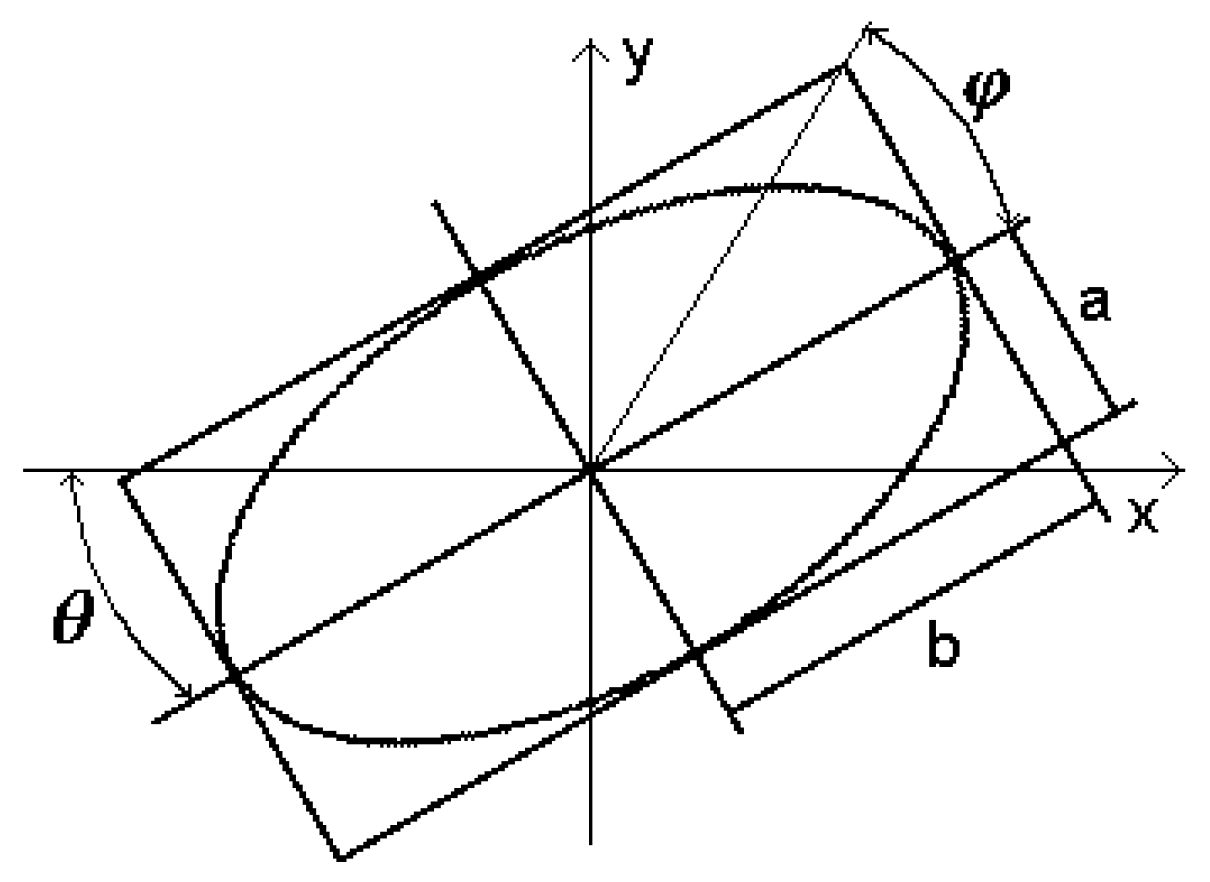
To quantitatively describe the principles of EMW polarization, the conception of the polarization ellipse is used [1] (see Appendix A.1).
During the reflection of an electromagnetic wave by a radar-sensed object, the electromagnetic field , which surrounds the object, contains two waves—the incident and reflected (scattered) . If we consider the fields and directly near the object, then, due to the vector representation of the fields, both the incident and scattered fields contain, in the general case, two orthogonally polarized components, which are represented on the orthogonal polarization basis in the form of .
Appendix A describes the process of EMW scattering and the concept of a polarization scattering matrix (PSM).
When receiving a signal with arbitrary ellipticity and orientation, dual-channel polarization reception is necessary to obtain the full power of the reflected signal, which is important for solving the problem of detecting low-visibility radar objects.
The independence of the PSM in the form given in Appendix A.2, from the polarization basis can be achieved by its representation through its eigenvalues , and eigenvectors [28], which are determined by the characteristic equation
and have the following form:
where and are the polarization parameters of the so-called [27] object’s own polarization. Physically, the eigenpolarizations in Equation (5), corresponding to the eigenvalues in Equation (4) of the matrix in the form (see Appendix A.2), are characterized by the absence of the reflected signal of the components that are orthogonally polarized to the irradiating wave. In this case, the eigenvalues , , of the PSM represent the complex reflection coefficients of an object when probed with signals corresponding to its own polarizations. Moreover, the eigenvectors in Equation (5), corresponding to the PSM eigenvalues , , are orthogonal by definition and form the proper in-phase orthogonally elliptical polarization basis of the object, in which the reflected signal is maximized. Furthermore, the matrices in Equations (4) and (5) do not depend on emitted and received polarization.
2.2. Polarization Selection of Radar Objects
Actual radar signals reflected by the Earth’s surface, vegetation and buildings have random polarization, which depends on the shape of the object’s surface, its dielectric constant and conductivity. Weak levels of signals reflected from power lines should be detected against the background of the receiver’s own noise and strong reflection from the underlying surface. The receiver’s own noise can be considered randomly polarized, and reflections from the Earth’s surface have a particular polarization structure with unknown parameters. At the same time, signals reflected by power lines correspond to the polarization scattering matrix in the form , which is given in Appendix A.2. Consequently, it is possible to detect the reflected signals against the background of noise and interference [29].
The emitted signal has the following structure:
where is a function that describes the shape of a complex signal envelope with respect to the time variable ; is the polarization index, which corresponds to the polarization of the sensing signal—vertical or horizontal ; and is the carrier frequency of the signal oscillation.
The received signal is a mixture of useful signals , the interference reflection from the Earth’s surface and the internal receiver noise :
where is the corresponding PSM in the form (see Appendix A.2), which describes the reflection characteristics of radar observation objects depending on the polarization of radiation .
The components of the vector defined in Equation (7) correspond to the type of polarization of oscillations at the receiver input for a given polarization of radiation .
Solving the problem of the polarization selection of signals against the background of interference requires the consideration of the corresponding distinctive features. The signal reflected from power lines has sufficiently pronounced polarization, unlike signals reflected from the Earth’s surface. Passive interference from the Earth’s surface can be represented in the following form:
where is the proportionality coefficient, which takes into account factors such as signal losses during their propagation and signal transmission through antenna-feeder systems; is the antenna radiation pattern that forms on the surface of the area of its illumination; and are scattered and incident field strengths on an elementary surface area ; and is the delay time in signal propagation related to distance .
The geometry of the formation of signals reflected by the surface is shown in Figure 1.
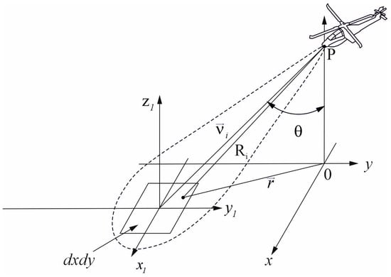
Figure 1.
Geometry of formation of signals reflected from surfaces and objects.
The problem of optimizing the signal selection method in a polarimetric radar can be represented via the maximum likelihood method [24] by solving the following equation:
where is the likelihood function. The solution of Equation (9) is presented in Appendix B.1.
Given the development of the equation, it becomes clear that we should look for the maximum of the multiplier or a directly related output effect . In coordinate form, the output effect is expressed as follows:
where is the delay time associated with the distance to the observed objects.
The internal receiver noise can be considered white noise, independent of other noise and independent of passive interference from the Earth’s surface .
Furthermore, it is necessary to consider the energy parameters using the correlation matrix of the receiver’s internal noise, described in Appendix B.2, to construct the output effect.
Since the Fourier transformation of the convolution is equal to the product of the images, Equation (10) can be written in the following form considering the energy spectra given in Appendix B.2:
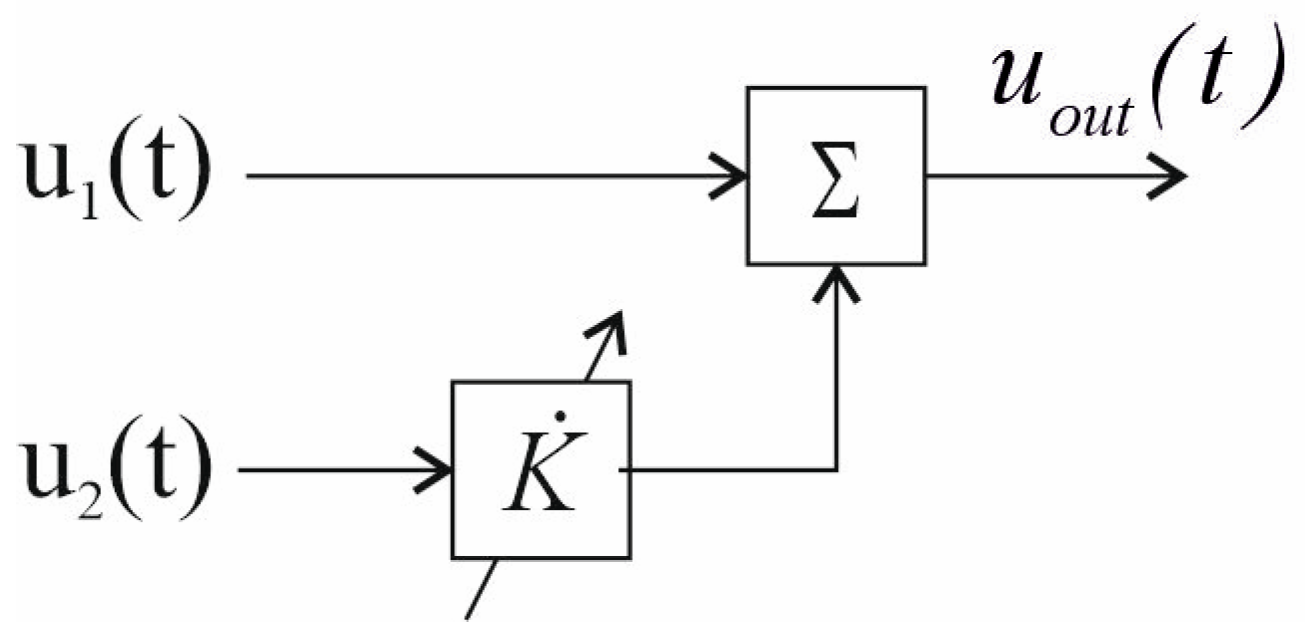
The analysis of Equation (11) shows that correlated interference can be compensated in a radar system with the separation of the electromagnetic wave into two polarization-orthogonal components, for example, horizontal () and vertical (), with dual-channel reception due to the so-called virtual Poelman adaptation [30] (Figure 2). The input signals of orthogonal components of electromagnetic waves are summed with a weighting factor , which is selected to ensure the equalization of the amplitudes at the input of the adder for further compensation. In the technical implementation of the circuit shown in Figure 2, it is necessary to adjust the complex transmission coefficient using the correlation processing of signals in polarization-orthogonal channels.
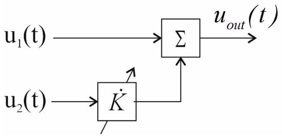
Figure 2.
Poelman’s principle of virtual adaptive selection.
Some assumptions and simplifications were made to obtain a method for the optimal polarization selection of a polarization-anisotropic object against a polarization-isotropic background.
Let us assume that both channels of the receiver are identical, which means that the internal noise of the receivers is equal in variance, with . Then, the received signals have a similar structure and differ only by coefficient, as can be observed in the following expression:
where an intensity factor, which represents a real value.
As observed in Appendix B.3, the output effect of the polarization interference compensator is denoted as
where
The part in Equation (13) performs passive interference compensation by subtracting signals with a different polarization and considering the weighting coefficients (14) and (15), and the multiplier provides matched filtering. This method requires the preliminary estimation of parameters in Equations (14) and (15), or the ensuring of their measurement in real time.
Signals and , which are written in Equation (13) in the form of spectral functions and , contain in their structure the following: informative signals, the internal noise of the receiver and passive interference reflected from the Earth’s surface. Therefore, to apply Equation (13), it is necessary to determine the intensity multiplier in real time , which is unknown.
In the absence of polarization-anisotropic objects, the radar observes only interference from the underlying surface, with or , where denotes a random process with variance equal to 1. Considering this condition and the calculation in Appendix B.4, the output effect is represented by the following formula:
Consequently, Equation (16) can be represented in the form
Let us introduce coefficient ; then,
Considering that the variances , and correlation coefficient are spatial functions and have a time dependence, the method of the optimal polarization selection of a polarization-anisotropic object against a polarization-isotropic background is written in the form
where is the residual from interference, which is not compensated by the algorithm. This residual should theoretically be zero when observing a homogeneous polarization-isotropic surface. The term is the variance ratio of and for signals in the orthogonal polarization receiving channels and , and is the correlation coefficient of signals in two orthogonal polarization receiving channels.
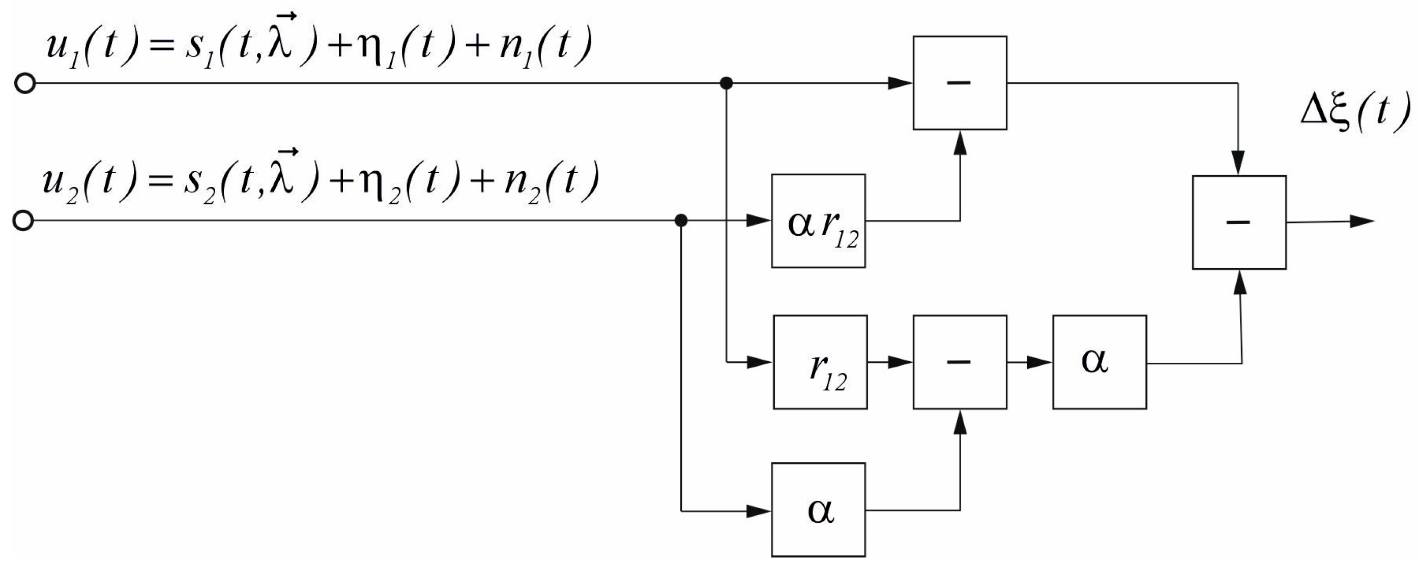
The resulting method corresponds to the structural diagram of the polarization signal selector shown in Figure 3.

Figure 3.
Structural diagram of the optimal method of polarization selection for polarization-anisotropic objects on a polarization-isotropic background.
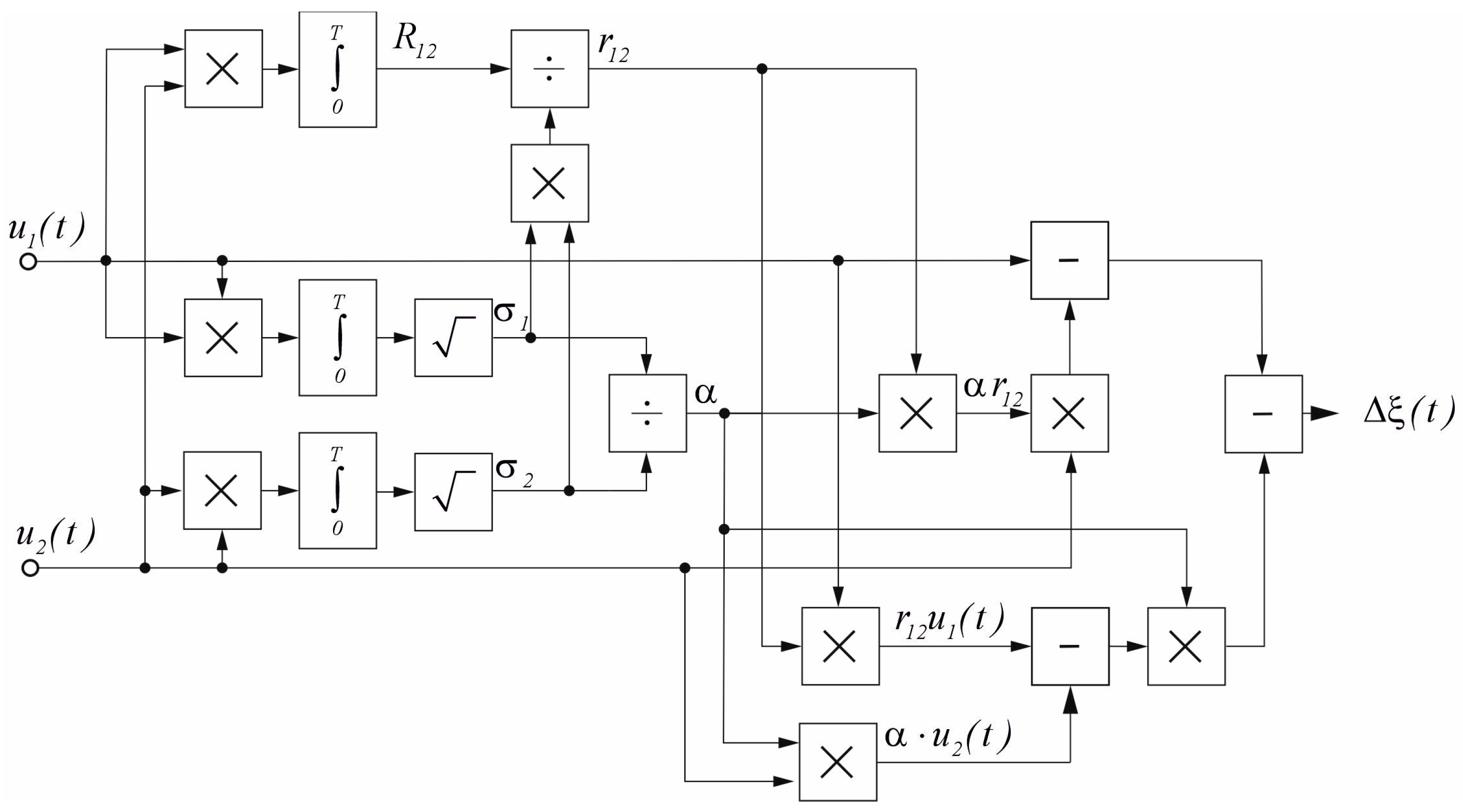
For the practical implementation of the theoretical method, a signal processing algorithm was developed in a digital signal processor (DSP), shown in Figure 4.
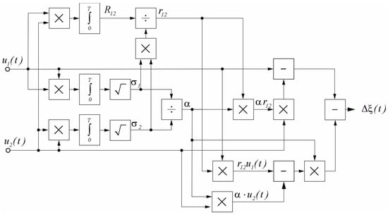
Figure 4.
Structural diagram of the sequence of operations for DSP implementation.
The input of the signal processor algorithm shown in Figure 4 should be supplemented directly with the output signals of dual-channel polarization radar receiver—for instance, when the radar operates in circular polarization—or with the results of the eigenvalue calculations (see Equation (4)) obtained from measurements on an arbitrary polarization basis of the PSM (see Appendix A.2). The algorithm shown in Figure 4, in the time interval , calculates variance estimations , and signals in polarization-orthogonal reception channels. Additionally, this algorithm calculates the correlation coefficient between polarization channels and the adaptation coefficient that computes the output signal , in which interference from the underlying surface and local spatially distributed objects should be suppressed. The signal reflected by a small polarization-anisotropic object should retain its amplitude. The output signal should be superimposed on the image of the terrain obtained by the radar to highlight the present invisible objects endangering the flight.
The constant of integration provides the adaptability of the algorithm. The adaptability coefficient and the correlation coefficient depend on time and the constant of integration , which should be determined by computer modeling considering the technical characteristics of the radar.
3. Results
This section presents simulation modeling results for a certain surface model and signals formed during reflection. Experiments using a polarization radar system in actual environmental conditions to confirm the surface model’s adequacy and the developed algorithm’s performance are also described. Based on the experiments’ results, polarimetric images were reconstructed, and various processing methods were compared.
3.1. Method and Results of Computer Modeling
The shape and polarization characteristics of the reflected radar signal depend on many factors, namely, the parameters of the radar (length of the radiated wave, width of the radiation pattern, duration and shape of the pulse) and the conditions of observation (angle, distance to the object, angle of site and azimuth, polarization of sensing and reception). Also, the reflected radar signal’s characteristics depend on the object’s profile and its electrophysical properties (dielectric permeability and conductivity). All the listed factors must be considered when modeling polarimetric signals to obtain reliable results.
Nowadays, various methods are used to model signals reflected by the underlying surface [31]—the two-scale scattering model is the most common [32,33], as well as the combined approach [34,35], which uses a combination of several methods.
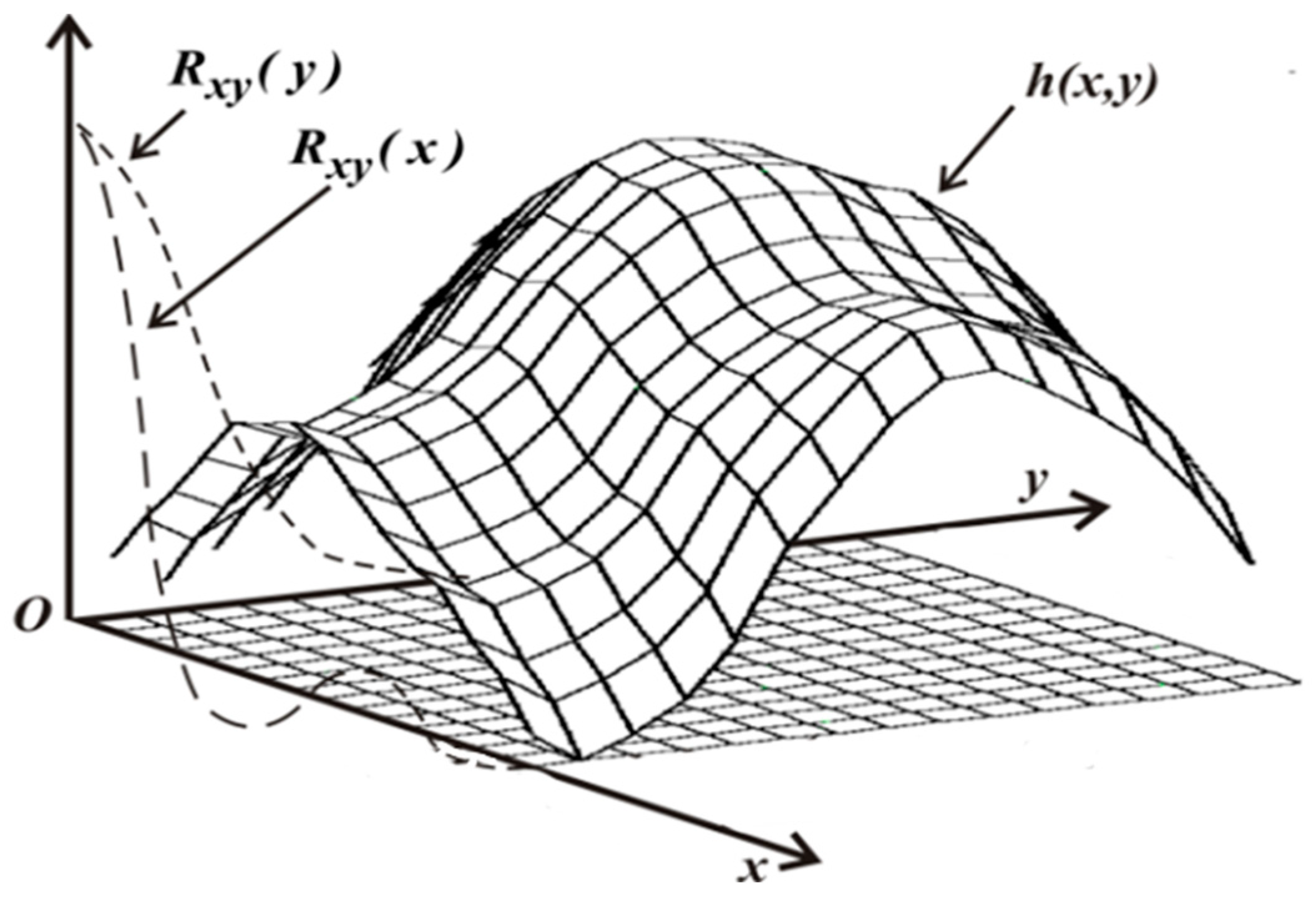
We employed a multi-scale model of surface heights to model radar signals reflected by the underlying surface [36]. In this model, the Earth’s surface is represented as a randomly connected surface of elementary facets, as shown in Figure 5, having a given correlation structure , corresponding to the type of surface (water surface, flat sand and rough terrain, among others). The geometric dimensions of the facets are much smaller than the wavelength of the radar signal.
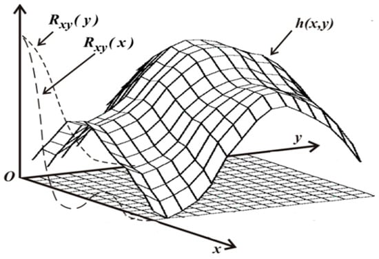
Figure 5.
General view of the surface model.
For a given flight altitude and radar parameters (width of the radiation pattern, operating frequency, pulse duration and polarization of radiation, among others), the distances to each of the elementary facets of the surface and their observation angles are calculated (Figure 1). For each elementary site, the reflection coefficients of electromagnetic waves are calculated using the Fresnel coefficients, considering the orientation of each facet relative to the radar and the given electrophysical properties of the surface (complex permittivity). Each point on the surface is considered a source of secondary waves. The signal reflected in the direction of the radar is calculated as a set of complex signals reflected by each facet, considering the distance to them and the shading of individual surface sections [37] according to Equation (8).
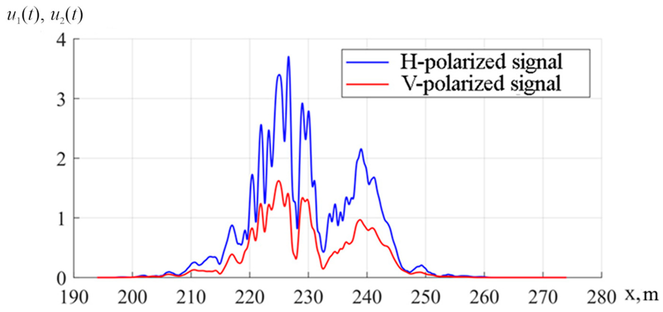
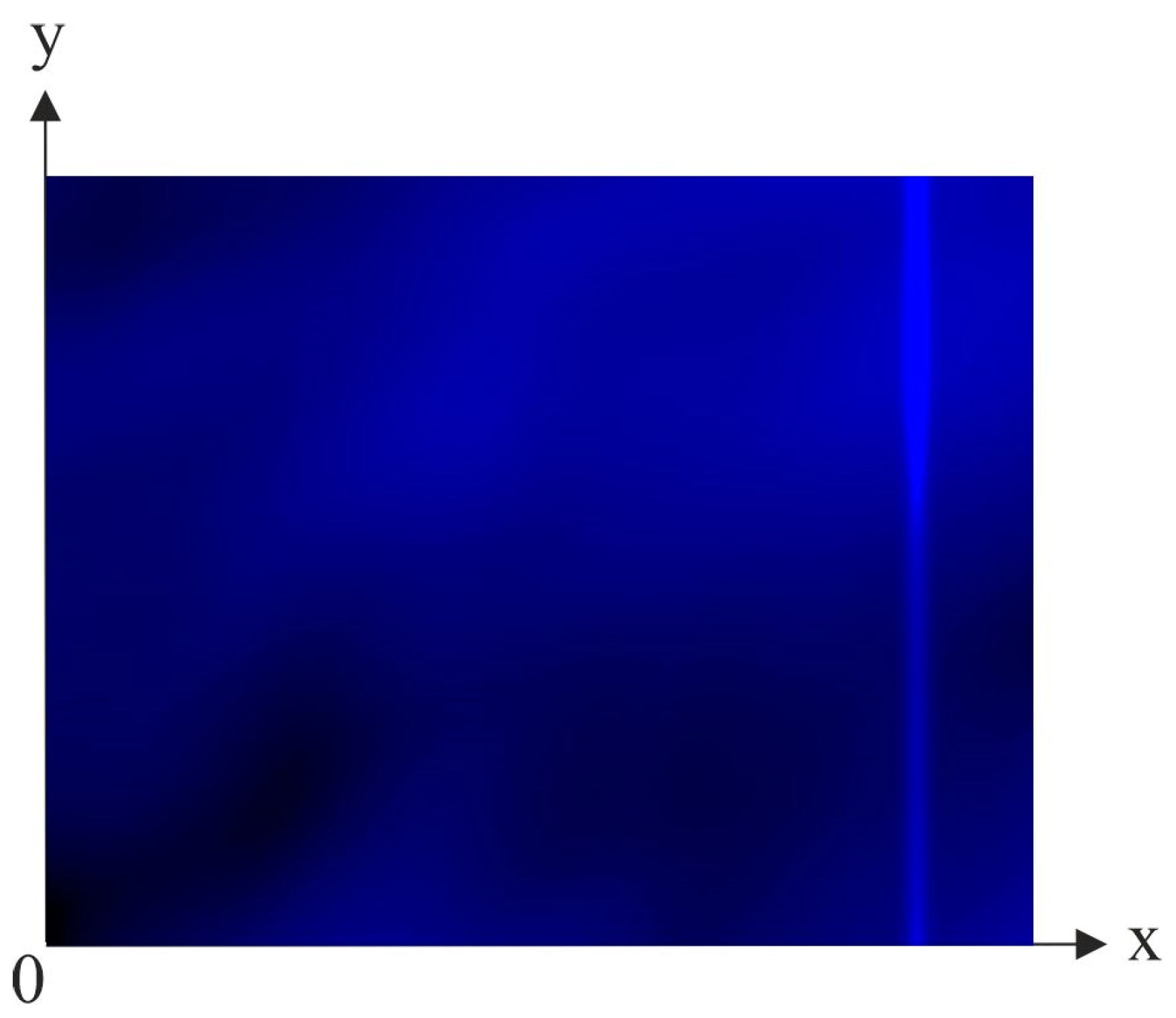
The resulting spatial–temporal distribution of electromagnetic waves is divided into two orthogonally polarized components according to the orientation of the radar antenna in space. The processing procedure of the radar signals is subjected to time discretization according to the sampling frequency of the radar’s analog-to-digital converters, considering its amplitude, frequency and noise characteristics. The methodology in [38] is taken as a basis for simulating signals in the and channels reflected from the surface and received by radar. An example of a surface fragment with elevation differences of ±0.1 m and a pixel size of 1 mm 1 mm is shown in Figure 6. Figure 7 shows the received signals in the and channels of the receiver as a result of modeling the signals reflected by such a surface. In Figure 7, represents an
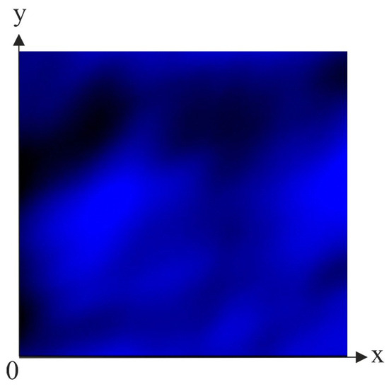
Figure 6.
Fragment of a surface model.

Figure 7.
A signal reflected by the surface.
H-polarized signal and represents a V-polarized signal.
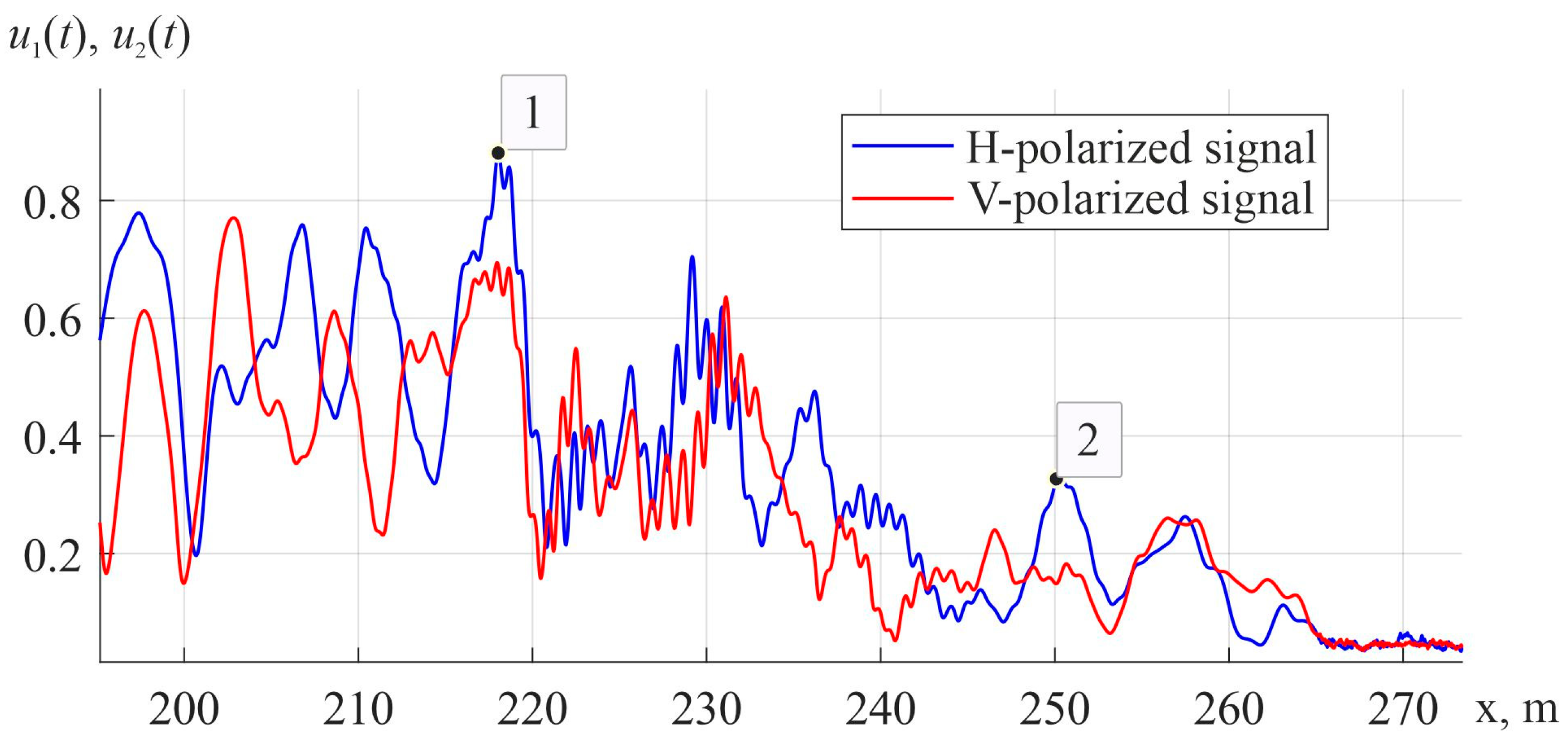
To test the algorithm’s effectiveness for detecting polarization-anisotropic objects against the background of the Earth’s surface, signals reflected by a power line wire with a diameter of 32 mm, placed above the surface at a height of 10 m, were simulated. A fragment of the Earth’s surface with power lines with a height difference of ±0.1 m is shown in Figure 8. One pixel on this picture has a surface measuring 1 mm 1 mm. To calculate the reflected signals, a well-known model [39] of radar signal reflection by power line wires was used, considering the influence of the underlying surface [40] and the presence of noise from radar receivers. An example of signals in the and channels of the radar receiver is shown in Figure 9. In this figure, at a distance of 218 m, the maximum level of interference from the underlying surface is observed (position 1). The amplitude of the signals in the and channels reflected by the power line wire at a distance of 250 m (position 2) is three times smaller than the maximum reflection from the underlying surface.

Figure 8.
Fragment of the Earth’s surface model with power lines.
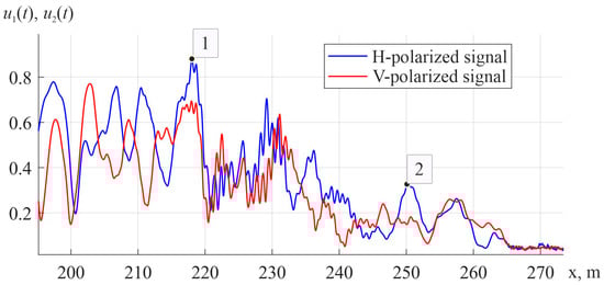
Figure 9.
Received signals from the Earth’s surface (label 1) and power line (label 2).
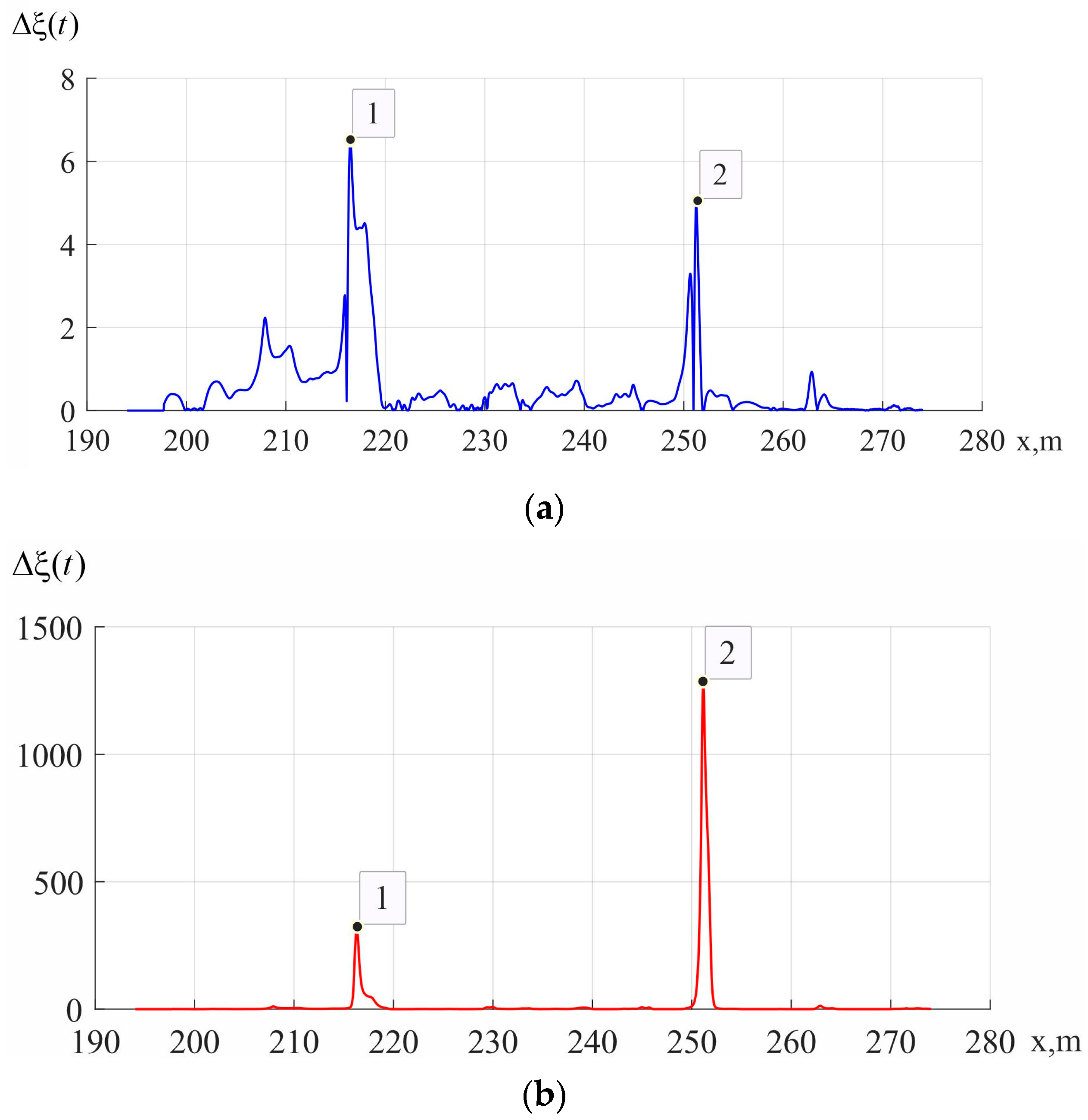
The adaptive polarization selection method was simulated for a wire with a diameter of 32 mm at a distance of 250 m against the background of the underlying surface. The simulation was carried out for two radar variants—with circular polarization in radiation and dual-channel polarization reception on an , basis; and with , radiation modulation and polarization dual-channel reception on an , basis with the measurement of the polarization scattering matrix (see Appendix A.2) and its eigenvalues , presented in Equation (4). The simulation results are shown in Figure 10, where Figure 10a shows the result of processing by the algorithm that utilizes the output signals of the receiver (, —channels) with circular polarization in sensing. The figure shows that this algorithm does not sufficiently suppress reflections from the Earth’s surface (labeled as 1), but although these reflections are present, the power line wires (labeled as 2) can be observed. Figure 10b shows the result of processing by the algorithm using Equation (18) and eigenvalue processing , ). In this case, the algorithm better suppresses reflections from the Earth’s surface (label 1), and the output signal at the point of placement of the power line (label 2) significantly exceeds the signals from the Earth’s surface.
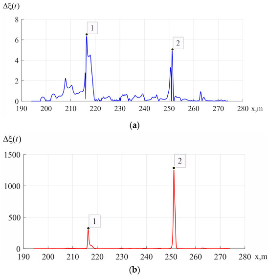
Figure 10.
Results of polarization selection of a power line with (a) circular polarization in sensing and (b) full-polarization sensing and eigenvalue signal processing. Labels 1 and 2 represent the position of the corresponding labels in Figure 9.
The simulation experiment results demonstrated significantly higher efficiency when eigenvalue signal processing was used compared to the variant of circular-polarization sensing. Nonetheless, this requires experimental verification in full-scale conditions.
3.2. Experimental Equipment
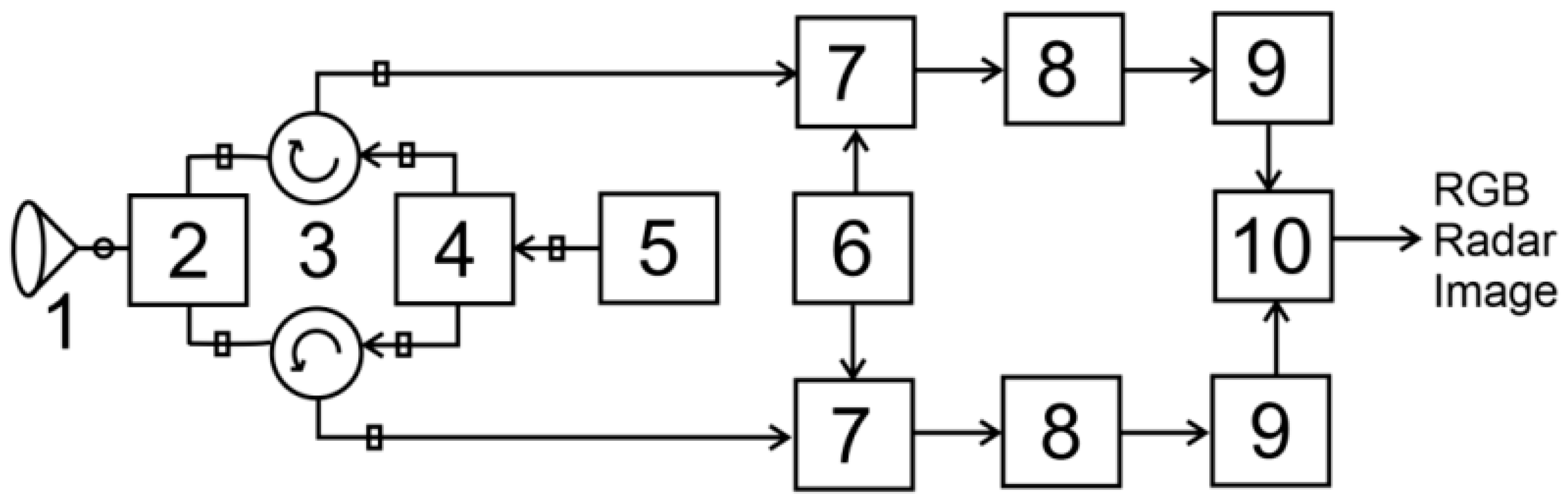
For experimental studies, a W-band radar (Figure 11) was developed with a polarization-isotropic antenna diameter of 120 mm and an orthomode converter separating the received signal into vertically and horizontally polarized components. Through the circulators of and , a pulse transmitter with a power of 5 W, a duration of 50 ns and a frequency of 94 GHz is connected to the channels of the orthomode converter. The switch ensures the connection of the transmitter either alternately to and channels or simultaneously. At the same time, a signal with circular polarization is emitted.
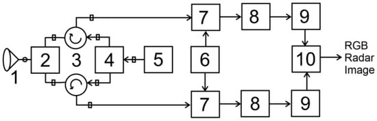
Figure 11.
Structure of the experimental radar. 1—Cassegrain Reflector Antenna; 2—Orthomode Transducer; 3—Y-Junction Circulators; 4—Pin Diode Switch; 5—pulse transmitter; 6—Phase-Locked Oscillator; 7—Mixers; 8—intermediate-frequency amplifier with logarithmic detector; 9—analog-to-digital converter; 10—digital signal processor.
The reflected signal is divided into and components, which are transferred by mixers to an intermediate frequency of 2.2 GHz, amplified at an intermediate frequency and detected by logarithmic detectors. Video pulses are converted into digital format by analog-to-digital converters ADS4229 with a sampling frequency of 250 MHz and processed by a signal processor, which is implemented on the FPGA XC7A50T-2FGG484I of the Artix-7 family. This ADC generates a data stream of 6 Gbit/s. The processing of such a signal cannot be performed in real time using a classical DSP, which is why an FPGA was used as a processor. A feature of the FPGA is that the algorithm is built directly on the structure of the internal connections of the microcircuit. In this case, a possible indicator of the complexity of the implemented algorithm is the number of slices (basic structural units of the FPGA) used in the FPGA. Thus, the proposed algorithm occupied 5,645,643 slices, and this number will not significantly differ when using another microcircuit. The total delay for obtaining the calculation result is about 3584 clock cycles, which, at a frequency of receipt of compartments of 250 MHz, is about 14.3 μs. Using the performance of such an FPGA allowed the experiment to be conducted in real time during flight time and helped the pilot observe dangerous objects without delay.
The radar is placed in a housing with a built-in scanning mechanism in the 30° azimuth sector and a software-controlled tilt angle.
3.3. Experimental Results
For experimental verification of the developed methods of signal processing, a full-scale experiment was conducted to measure the reflected signals, process them in real time by a signal processor used in the radar system and reconstruct synthetic polarimetric images of the terrain when sensing it with a circularly polarized signal and a polarization-modulated signal. The objectives of the experiment are listed as follows:
- To obtain synthetic polarization images during terrain probing with a circular polarization signal and synchronous reception of orthogonally polarized reflected signals , , and to visualize their amplitude in GB channels of the RGB image.
- To apply the polarization selection algorithm based on Equation (18) to signals , , and to visualize the result of polarization selection in the R channel of the RGB image.
- To obtain synthetic polarization images during terrain probing with a signal with polarization modulation and synchronous reception of orthogonally polarized reflected signals. Then, to perform the reconstruction based on the measurements of the polarization scattering matrix (see Appendix A.2) as well as the calculation of eigenvalues in each image element , (see Equation (4)) and to visualize their amplitudes in GB channels of the RGB image.
- To apply the previously mentioned polarization selection algorithm to signals , , and to visualize the result of polarization selection in the R channel of the RGB image.
- To compare the information content of the images obtained by the two methods.
- To evaluate the performance and efficiency of the polarization selection method using directly measured signals in polarization-orthogonal channels and using eigenvalues in signal processing.
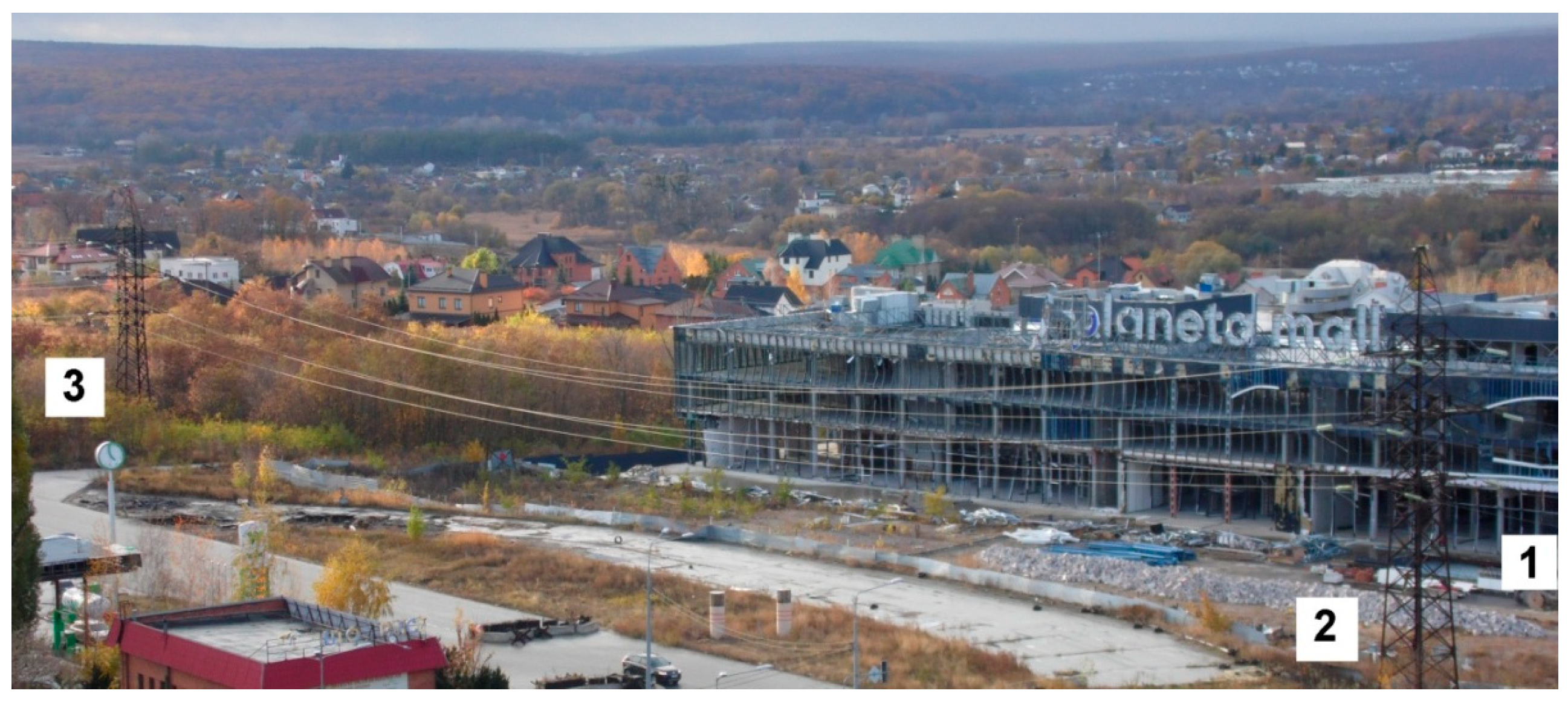
The scene shown in Figure 12 was chosen for the experiments. It contains a large building (labeled as 1), transmission line supports (labeled as 2 and 3), wires between them and vegetation. The radar was placed at a height of 37 m above ground level; the terrain was scanned in a 30° sector. The distance to the nearest point of the building (label 1) was 278 m, while the transmission lines labeled 2 and 3 were at 208 and 383 m, respectively.
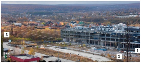
Figure 12.
Scene for constructing a radar image. Label 1 represents the nearest point of the building, labels 2 and 3 are the transmission line supports.
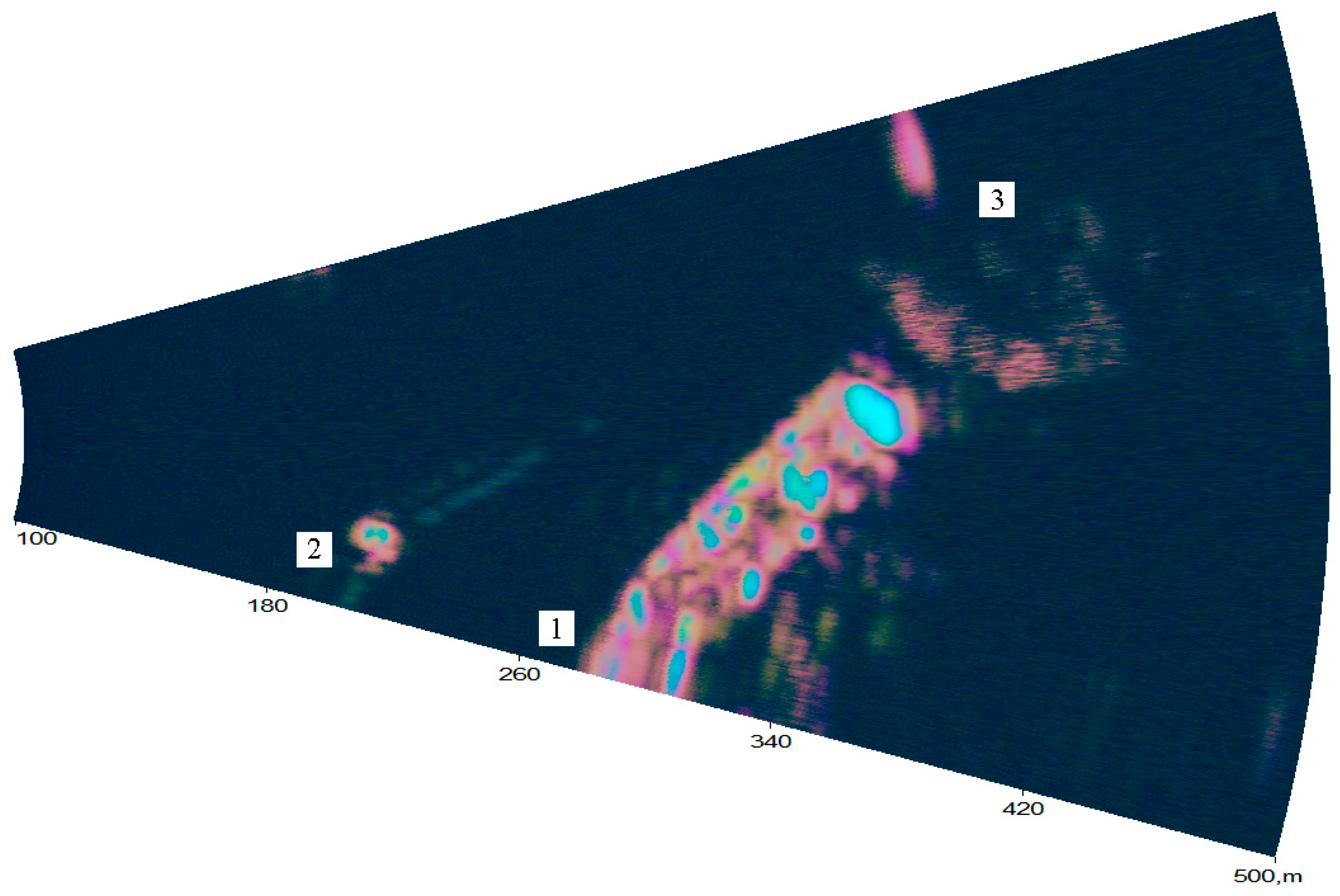
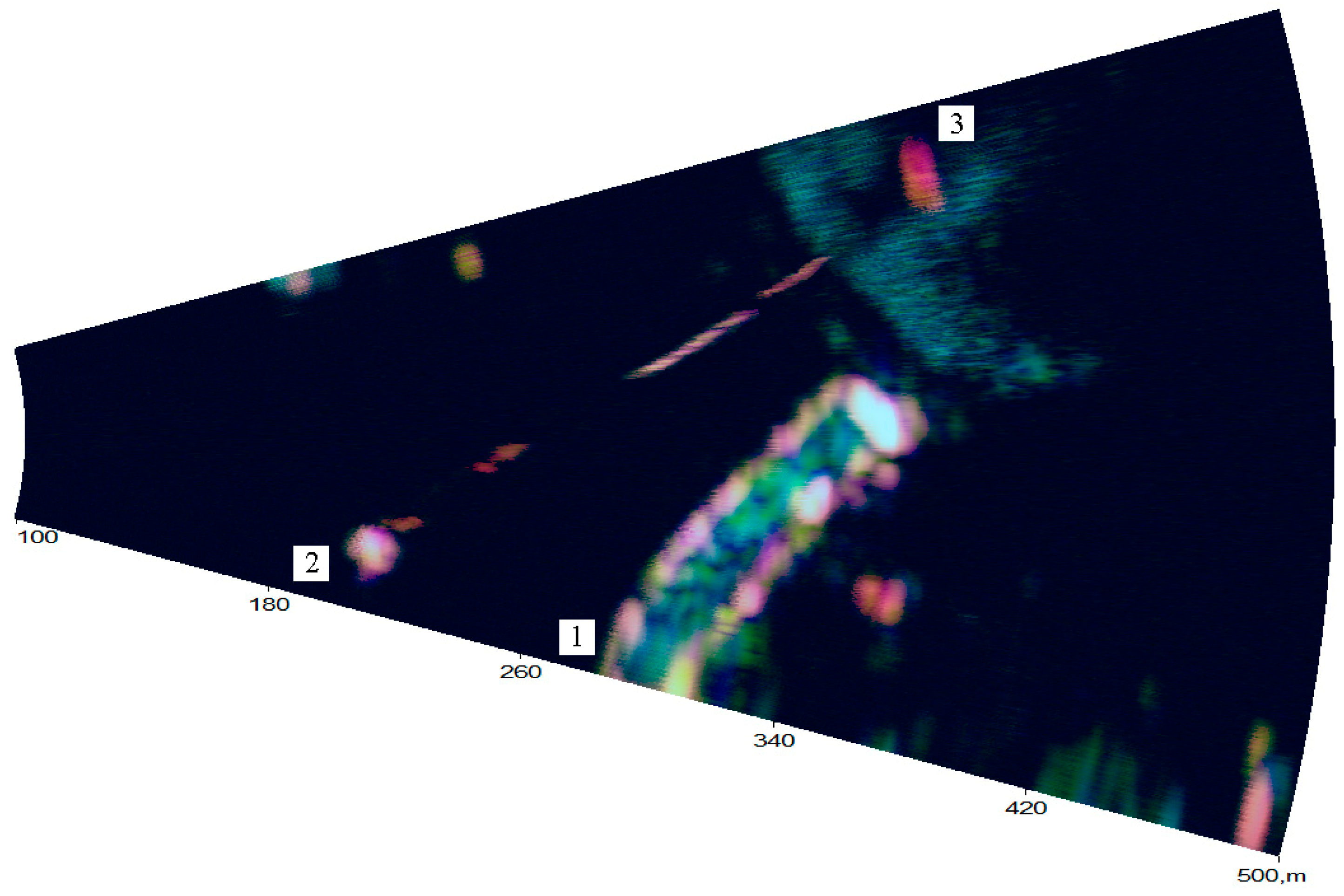
An example of a synthetic image of this area obtained during its probing with a circular polarization signal, with received orthogonally polarized signals, is shown in Figure 13. In contrast, a synthetic image from the polarization-modulated signal with the measurement of the polarization scattering matrix and visualization of its eigenvalues is given in Figure 14. The labels 1, 2 and 3 on the images mark the position of the objects shown in Figure 12. The result of the polarization selection of objects by the developed algorithm is displayed in the red channel of the RGB images.
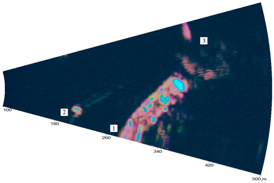
Figure 13.
Polarimetric image with circular polarization in sensing. The labels denote the objects described in Figure 12.
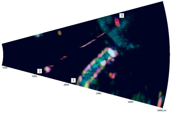
Figure 14.
Polarimetric image with eigenvalue signal processing. The labels denote the objects described in Figure 12.
An analysis of the experimental data shows that when using a circularly polarized signal for terrain sensing, the reflected signals “react” to the orientation of reflecting objects, which is manifested in a change in the color of the pixels in the image. At the same time, the power transmission line wires and support (label 3) are practically invisible. However, the radar’s energy potential is theoretically sufficient for their detection, as evidenced by the marks from objects, particularly vegetation, that can be seen at a greater distance.
The polarization selection algorithm selects practically all the objects observed in the image (see red highlights in Figure 13), regardless of their nature; i.e., in the process of sensing with a circular polarization signal, reflections from most objects are polarization-anisotropic. The use of eigenvalue signal processing (Figure 14) significantly (by at least 3 dB) reduces the noise level in the polarimetric image and gives the image more contrast. Figure 14, unlike Figure 13, shows that there are inconspicuous objects, in particular, power transmission line wires. The polarization differences in reflections from metal and concrete structural elements are noticeable on the roof of the building (the building has a metal fence around the perimeter of the roof). Furthermore, the reflections from vegetation are more noticeable. In addition, the detection range of objects at large distances increases.
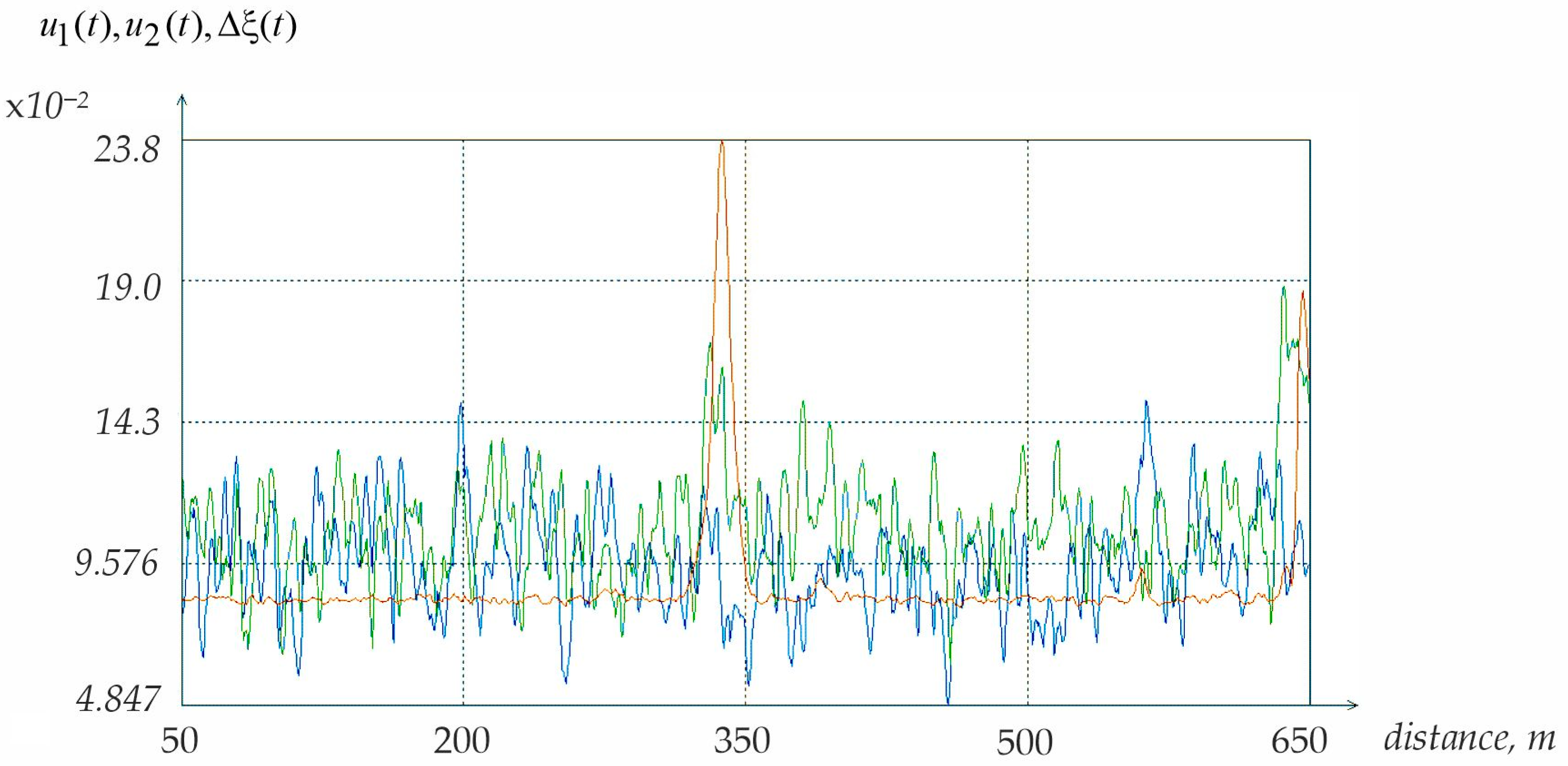
The polarization selection algorithm highlights building boundaries and poorly visible objects, such as poles and power transmission line wires (see red highlights in Figure 14). However, it ignores polarization-isotropic reflections from vegetation. As an example of the polarization selection algorithm’s operation, Figure 15 demonstrates a fragment of one row of the image shown in Figure 14. In this example, the pulses reflected from the power transmission line wires at 348 m (blue—vertical polarization; green—horizontal polarization) and the output signal of the polarization selector (red) are observed. It can be seen that using the adaptive algorithm allows for a significant reduction in the level of signal fluctuations and an increase in the probability of detecting low-visibility polarization-anisotropic radar objects. A point worth mentioning is that determining the numerical values of the probability of detecting power transmission line wires against the background of the Earth’s surface and objects requires further specialized experiments.
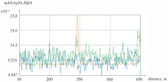
Figure 15.
Instantaneous realization of reflected signals. The red signal is the output signal of the polarization selector, and the blue and green signals are acquired correspondingly by vertical and horizontal polarization.
4. Discussion
One way to increase the safety of helicopter flights at low altitudes in difficult meteorological conditions is by employing onboard radars in the millimeter range of radio waves. Detecting inconspicuous obstacles, such as power lines, requires using radar polarimetry methods that allow their radar visibility to increase, since power lines have the property of polarization anisotropy.
The use of circular polarization in sensing partially reduces the dependence of the reflected transmission line signal’s power on its observation angle but results in the loss of at least half of the sounding signal’s power.
A more effective approach is the polarization modulation of the probing signal in combination with the reflected signals’ two-channel reception on an orthogonal polarization basis. The polarization scattering matrix measured at the same time contains all the power of the reflected signal but depends on the viewing angle of the radar object. This dependence can be eliminated by calculating in real time the eigenvalues of the polarization matrix of scattering, which are invariant to the orientation of the radar target in the plane of incidence of the electromagnetic wave. The two signals obtained in this case, corresponding to the two eigenvalues of the polarization scattering matrix, are polarization-orthogonal, depending on the shape of the radar object, and can be used for the polarization selection of inconspicuous radar targets against the background of the Earth’s surface.
The polarization radar characteristics of the Earth’s surface, vegetation and ground objects, such as buildings and other constructions, including transmission lines, are not sufficiently studied today in the millimeter range of radio waves. Therefore, for selecting inconspicuous objects against the background of the Earth’s surface, an adaptive algorithm of polarization selection is proposed, analytically obtained under the assumption that the polarization characteristics of power lines are different from the polarization properties of the underlying surface.
Assessing the performance of the developed algorithm for processing signals received by polarimetric radar using computer modeling methods showed its effectiveness on data obtained by known methods.
For experimental studies, a prototype of a helicopter polarimetric radar capable of emitting signals both under circular polarization conditions and with polarization modulation was designed.
The two-channel polarization reception of reflected signals allows for the reception of their full power. The hardware algorithm for adaptive polarization selection was implemented using the DSP-reconstructed eigenvalue signals. The radar primarily scans the environment and obtains a radar color image that visualizes the helicopter’s position for the pilot, as well as the location of objects on the terrain and their polarization properties. The reconstruction of an image that represents the results of polarization selection in the red channel of the RGB image allows focus on inconspicuous objects that differ in their polarization properties from the surrounding terrain and, as a result, the detection of obstacles that are dangerous for flight with a high probability.
Developing a dataset that can characterize such objects based on their electrophysical properties would allow the problem of recognizing radar objects on polarimetric radar images to be investigated in the future. The results obtained in this study show the prospects of this area of research.
A limitation of the adaptive polarization selection method is the signal-to-noise ratio (SNR), which must be . This condition limits the ability to detect thin wires whose diameter is smaller than the radar wavelength, particularly 3 mm. A common problem for W-band radars is the presence of intense precipitation on the signal propagation path, both causing signal attenuation in water and creating powerful interference reflections.
5. Conclusions
Polarimetric radar system tests in actual environmental conditions have shown that the radar operating mode with polarization-modulated signal emission followed by eigenvalue signal processing provides higher-contrast and more informative radar images of the terrain than when using only circular polarization in sensing. In addition, adaptive polarization selection identifies low-visibility radar objects more effectively when using preliminary eigenvalue signal processing against another variant that directly uses the radar receiver’s output signals.
The results of the conducted experimental studies have shown that further efforts should be directed at studying the polarization characteristics of real radar objects, such as the Earth’s surface, vegetation of various types, buildings, structures and equipment.
Author Contributions
Methodology: M.B., H.C., V.K., A.P. and E.T.; formal analysis: M.B., H.C., V.K., V.P., A.P., S.S., B.G.-S. and E.T.; investigation: M.B., H.C., V.K., A.P. and E.T.; resources: V.P., data curation: M.B., H.C., V.K., A.P. and E.T.; writing—original draft preparation: H.C., V.K., A.P, V.P., B.G.-S. and E.T.; writing—review and editing: S.S., V.P. and B.G.-S. All authors have read and agreed to the published version of the manuscript.
Funding
This research received no external funding.
Data Availability Statement
The original contributions presented in the study are included in the article, and further inquiries can be directed to the corresponding author.
Acknowledgments
The authors would like to thank the National Aerospace University “Kharkiv Aviation Institute” (Ukraine), the Ivan Kozhedub Kharkiv National Air Force University (Ukraine), Instituto Mexicano del Petroleo (Mexico), Instituto Politecnico Nacional (IPN) (Mexico), Comision de Operacion y Fomento de Actividades Academicas (COFAA) of IPN and Secretaria de Ciencia, Humanidades, Tecnologia e Innovacion (SECIHTI) (Mexico) for their support in this work.
Conflicts of Interest
The authors declare no conflicts of interest.
Abbreviations
The following abbreviations are used in this manuscript:
| DSP | Digital Signal Processor |
| EMW | Electromagnetic Waves |
| FPGA | Field-Programmable Gate Array |
| PSM | Polarization Scattering Matrix |
| RCS | Radar Cross-Section |
| SNR | Signal-to-Noise Ratio |
Appendix A
Appendix A.1. Polarization Ellipse Parameters
To quantitatively describe the polarization of EMWs, the geometric parameters (ellipticity angle and orientation angle ) of the polarization ellipse (Figure A1) are used [1], with the value of the ellipticity angle being as follows:
where and are semi-major and semi-minor axes of an ellipse; and the orientation angle is the angle between ort and the semi-major axis of the ellipse, limited by the range .
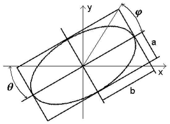
Figure A1.
Polarization ellipse.
Figure A1.
Polarization ellipse.
Appendix A.2. Polarization Scattering Matrix
To describe the relationship between the scattered and the incident fields, the use of four complex values is required:
which form the so-called polarization scattering matrix (PSM) of size [27] as follows:
which describes the reflective properties of an object for orthogonal polarizations .
However, the values of the PSM elements depend on the choice of orthogonal polarizations and the angles of object observation.
In radar, an orthogonal-linear polarization basis is usually used, which consists of vertical () and horizontal () polarization. The polarization characteristics of a radar object for a given polarization basis are described by the PSM of the type
and, for the case of single-position radar, .
While the original linear polarization basis of the EMW is rotated by an angle , the PSM in Equation (A2) is transformed as
where
If we change the ellipticity of the polarization basis to an angle φ, the PSM of Equation (A2) is transformed as
where
In the general case of the transition from a polarization basis to the polarization basis , the PSM values in Equation (A2) are transformed as
Expression (A5) demonstrates the main problem of describing the polarization properties of a radar object using the PSM in Equation (A1)—the elements of the matrix depend on the mutual orientation in the plane of the wavefront of the radar antenna and the radar object.
Let us consider the simplest example that illustrates the problem of the radar measurement of signals reflected by an object. Suppose the object of radar sounding on the polarization basis is a linear wire oriented in the plane at an angle relative to the axis . The theoretical PSM of such an object is well known:
where is the electrical wire length.
If , with the wire oriented horizontally, then matrix (A6) takes the form
and according to (A2), the radar will receive the reflected signal only with the horizontal polarization of sensing and reception.
For a vertically oriented object, such as a telecommunications tower, the angle , and the theoretical matrix (A6) will take the form
The radar will only receive the reflected signal when sensing and receiving are vertically polarized.
When the radar operates in circular polarization, the angle in Equation (A4) will have the value . When sensing a polarization-anisotropic object with the PSM in Equation (A6) according to Equation (A4), we will receive only half of the power of the circularly polarized signal upon reflection.
Thus, the presence of polarization anisotropy in signals reflected from several objects, which may pose a threat to flight safety, requires a change in the radiation’s polarization for the stable detection of such objects, in particular the angle of signal orientation , by an amount that is at least approximately equal to 90°.
Appendix B
Appendix B.1. Development of Output Effect
In Equation (9), is the likelihood function, which has the following form:
where is the matrix of inverse correlation functions.
The inverse matrix of correlation functions can be obtained from the integral-matrix inversion equation:
where is a correlation matrix, is an identity matrix and denotes the Dirac delta function.
Let us represent the function (A7) in the following form:
where
The function , which depends on the signal and noise energy ratio, does not depend on the parameters , since its main parameters are not energetic and can be considered a constant. Therefore, to solve Equation (9), we should look for the maximum of the multiplier or a directly related output effect .
Appendix B.2. Development Matrix of Energy Spectra
The interference correlation matrix can be written as the sum of the corresponding matrices:
and the correlation matrix of internal noises that are independent of each other is given in the form
Let us rewrite Equation (A8) considering the introduced simplifications:
where .
Equation (A12) is a convolution equation that can be solved using the Fourier transform:
where is an interference energy spectrum in matrix form.
Applying the Fourier transform to the matrix of correlation functions given in Equation (A11), we obtain the matrix of interference energy spectra.
In Equation (A14), and are equal, and spectra and, according to the Fourier transforms of the autocorrelation functions, are considered real numbers. Based on this, it can be concluded that .
The inverse matrix of energy spectra is found using Equation (A13) and has the following form:
where
is a determinant of the matrix of energy spectra.
Appendix B.3. Development of Output Effect
The output effect of the polarization interference compensator in Equation (11) can be rewritten in the following form:
Appendix B.4. Development of Equation (16)
The correlation function of such processes can be written as
where is determined by the observed surface profile.
Then, the output effect of the polarization interference compensator in Equation (13) can be represented as
Assuming that there is no receiver noise, which is acceptable with a high signal-to-noise ratio, the output effect of the polarization interference compensator is as follows:
Considering that the Fourier transform is a linear operation, and the addition and subtraction operations can be performed independently of the integration operation, the residual non-compensated interference given in Equation (A18) can be defined as
Expression (A19) can be represented in the following form:
Let us find the minimum of the variance in Equation (A20):
The next step is to calculate the derivative of Equation (A21) and set it equal to zero:
and then,
References
- McMillan, G.; Xu, H. Helicopter Aerial Work: Technology to Meet Growing Needs in Critical Missions. J. Am. Helicopter Soc. 2023, 69, 285–292. [Google Scholar] [CrossRef]
- International Civil Aviation Organization. Safety Report. Available online: https://www.icao.int/safety/Documents/ICAO_SR_2022.pdf (accessed on 15 August 2023).
- Jianjun, W.; Xiaoqian, M.; Jian, S.; Lei, L.; Jingang, Y.; Fengkai, Y. Research on Meteorological Early Warning Technology of Helicopter Patrol in High Altitude Area. In Proceedings of the 2020 International Conference on Computer Engineering and Application (ICCEA), Guangzhou, China, 18–20 March 2020; pp. 618–621. [Google Scholar] [CrossRef]
- Peng, Y.; Zhang, Z.; Zhu, X.; Fan, Y.; Wang, J.; Li, L. Research on Electrical Safety of Live-line Work of Ground Wire for UHV/EHV Transmission Line Based on Helicopter Winch Method. In Proceedings of the 2023 IEEE 6th International Electrical and Energy Conference (CIEEC), Hefei, China, 12–14 May 2023; pp. 2177–2182. [Google Scholar] [CrossRef]
- Chandrasekaran, R.; Payan, A.; Collins, K.; Mavris, D. Helicopter wire strike protection and prevention devices: Review, challenges, and recommendations. Aerosp. Sci. Technol. 2020, 98, 105665. [Google Scholar] [CrossRef]
- Valseca, V.; Paneque, J.; Martínez-de Dios, J.R.; Ollero, A. Real-time LiDAR-based semantic classification for powerline inspection. In Proceedings of the 2022 International Conference on Unmanned Aircraft Systems (ICUAS), Dubrovnik, Croatia, 21–24 June 2022; pp. 478–486. [Google Scholar] [CrossRef]
- Muñoz, D.F.T.; Prieto, F.; Correa, A.C. Power lines detection from a stereo vision system. In Proceedings of the 2020 5th International Conference on Control and Robotics Engineering (ICCRE), Osaka, Japan, 24–26 April 2020; pp. 242–245. [Google Scholar] [CrossRef]
- Xie, Z.; Zhang, G.; Fang, Z. Power line detection based on subpixel-neighborhood attention in complex terrain backgrounds. IEEE Sens. J. 2024, 24, 14493–14502. [Google Scholar] [CrossRef]
- Matikainen, L.; Lehtomäki, M.; Ahokas, E.; Hyyppä, J.; Karjalainen, M.; Jaakkola, A.; Kukko, A.; Heinonen, T. Remote sensing methods for power line corridor surveys. J. Photogramm. Remote Sens. 2016, 119, 10–31. [Google Scholar] [CrossRef]
- Zhencang, H.; Renjie, J.; Dong, L. A structural information aided method for intelligent detection of power line targets. In Proceedings of the 2023 IEEE 6th Information Technology, Networking, Electronic and Automation Control Conference (ITNEC), Chongqing, China, 24–26 February 2023; pp. 1622–1632. [Google Scholar] [CrossRef]
- Qian, J.; Mai, X.; Yuwen, X. Real-time power line safety distance detection system based on LOAM Slam. In Proceedings of the 2018 Chinese Automation Congress (CAC), Xi’an, China, 30 November–2 December 2018; pp. 3204–3208. [Google Scholar] [CrossRef]
- Shi, S.; Wang, S.; Li, T.; Liu, Y.; Sun, H. Numerical simulation of the radar cross section of UHV/EHV power lines illuminated by X-, C-, L-, and P-band spaceborne SAR. IEEE Trans. Geosci. Remote Sens. 2023, 61, 1–14. [Google Scholar] [CrossRef]
- Shi, S.; Liu, Y.; Cheng, L.; Chen, Z. Numerical simulation of the electromagnetic scattering characteristics of ultra-high voltage power line at X-band. In Proceedings of the 2020 IEEE 6th International Conference on Computer and Communications (ICCC), Chengdu, China, 11–14 December 2020; pp. 2289–2293. [Google Scholar] [CrossRef]
- Onana, V.-D.-P.; Kilic, O. A closed form radar cross section prediction modeling for overhead wires at millimeter waves. In Proceedings of the 2020 IEEE International Radar Conference (RADAR), Washington, DC, USA, 28–30 April 2020; pp. 180–185. [Google Scholar] [CrossRef]
- Chen, C.; Yang, F.; Hu, C.; Zhou, J. Power lines detection of 77 GHz millimeter wave radar based on synthetic aperture. In Proceedings of the International Conference on Radar Systems (RADAR 2022), Hybrid Conference, Edinburgh, UK, 24–27 October 2022; pp. 77–82. [Google Scholar] [CrossRef]
- Chen, C.; Zhou, J.; Yang, F. Power line detection method based on broadband characteristics of FMCW radar. In Proceedings of the 2022 14th International Conference on Signal Processing Systems (ICSPS), Zhenjiang, China, 18–20 November 2022; pp. 97–101. [Google Scholar] [CrossRef]
- Futatsumori, S.; Amielh, C.; Miyazaki, N.; Kobayashi, K.; Katsura, N. Helicopter flight evaluations of high-voltage power lines detection based on 76 GHz circular polarized millimeter-wave radar system. In Proceedings of the 2018 15th European Radar Conference (EuRAD), Madrid, Spain, 26–28 September 2018; pp. 218–221. [Google Scholar] [CrossRef]
- Futatsumori, S.; Miyazaki, N. Concept of helicopter all-around obstacle detection using millimeter-wave radar systems: Experiments with a beam-switching radar system and a multicopter. In Proceedings of the 2018 IEEE Asia-Pacific Conference on Antennas and Propagation (APCAP), Auckland, New Zealand, 5–8 August 2018; pp. 510–511. [Google Scholar] [CrossRef]
- Futatsumori, S.; Miyazaki, N. Ground reflection power measurements of thin high-voltage power lines using 76 GHz helicopter forward-looking low-transmitting power millimeter-wave radar. In Proceedings of the 2020 International Symposium on Antennas and Propagation (ISAP), Osaka, Japan, 25–28 January 2021; pp. 219–220. [Google Scholar] [CrossRef]
- Futatsumori, S.; Miyazaki, N. Bragg scattering characteristic evaluation of thin high-voltage power lines using low transmitting power helicopter forward-looking 76 GHz millimeter-wave radar. In Proceedings of the 2023 IEEE International Symposium on Antennas and Propagation (ISAP), Kuala Lumpur, Malaysia, 30 October–2 November 2023; pp. 1–2. [Google Scholar] [CrossRef]
- Ponomaryov, V.I.; Peralta-Fabi, R.; Popov, A.V.; Babakov, M.F. Detection and recognition of targets by using signal polarization properties. Autom. Target Recognit. IX 1999, 3718, 283–291. [Google Scholar] [CrossRef]
- Li, X.; Cheng, X.; Ju, X.; Peng, Y.; Hu, J.; Li, J. Optimization on the polarization and waveform of radar for better target detection performance under rainy condition. Remote Sens. 2024, 16, 2557. [Google Scholar] [CrossRef]
- Pavlikov, V.; Volosyuk, V.; Zhyla, S.; Kosharskyi, V.; Popov, A.; Odokienko, O. Optimization of polarization-Doppler selection of small-sized objects on the background of the Earth surface. In Proceedings of the 2022 IEEE 16th International Conference on Advanced Trends in Radioelectronics, Telecommunications and Computer Engineering (TCSET), Lviv-Slavske, Ukraine, 22–26 February 2022; pp. 559–563. [Google Scholar] [CrossRef]
- Volosyuk, V.; Zhyla, S.; Pavlikov, V.; Ruzhentsev, N.; Tserne, E.; Popov, A.; Shmatko, O.; Dergachov, K.; Havrylenko, O.; Ostroumov, I.; et al. Optimal method for polarization selection of stationary objects against the background of the Earth’s surface. Int. J. Electron. Telecommun. 2022, 68, 83–89. [Google Scholar] [CrossRef]
- Galletti, M.; Gekat, F.; Goelz, P.; Zrnic, D.S. Eigenvalue signal processing for phased-array weather radar polarimetry: Removing the bias induced by antenna coherent cross-channel coupling. In Proceedings of the 2013 IEEE International Symposium on Phased Array Systems and Technology, Waltham, MA, USA, 15–18 October 2013; pp. 502–509. [Google Scholar] [CrossRef]
- Popov, A.; Tserne, E.; Volosyuk, V.; Zhyla, S.; Pavlikov, V.; Ruzhentsev, N.; Dergachov, K.; Havrylenko, O.; Shmatko, O.; Averyanova, O.; et al. Invariant polarization signatures for recognition of hydrometeors by airborne weather radars. In Computational Science and Its Applications (ICCSA) 2023; Gervasi, O., Murgante, B., Taniar, D., Apduhan, B.O., Braga, A.C., Garau, C., Stratigea, A., Eds.; Athens, Greece, Lecture Notes in Computer Science; Springer: Cham, Switzerland, 2023; Volume 13956, pp. 201–217. [Google Scholar] [CrossRef]
- Yamaguchi, Y. Polarimetric SAR Imaging: Theory and Applications, 1st ed.; CRC Press: Boca Raton, FL, USA, 2020. [Google Scholar] [CrossRef]
- Li, D.; Zhang, Y. Unified Huynen phenomenological decomposition of radar targets and its classification applications. IEEE Trans. Geosci. Remote Sens. 2016, 54, 723–743. [Google Scholar] [CrossRef]
- Sarabandi, K.; Park, M. A radar cross-section model for power lines at millimeter-wave frequencies. IEEE Trans. Antennas Propag. 2003, 51, 2353–2360. [Google Scholar] [CrossRef]
- Poelman, A.J. Virtual polarisation adaptation–A method of increasing the detection capability of a radar system through polarisation-vector processing. IEEE Proc. Commun. Radar Signal Process. Part F 1981, 128, 261–270. [Google Scholar]
- Ticconi, F.; Pulvirenti, L.; Pierdicca, N. Models for scattering from rough surfaces. In Electromagnetic Waves; Zhurbenko, V., Ed.; InTech: Nappanee, IN, USA, 2011; pp. 203–226. [Google Scholar] [CrossRef]
- Song, D.-w.; Shang, S.; Luo, X. The study of microwave scattering of anisotropic sea surface with the corrected two-scale model. In Proceedings of the 2015 European Radar Conference (EuRAD), Paris, France, 9–11 September 2015; pp. 545–547. [Google Scholar] [CrossRef]
- Ye, J.; Wan, Y.; Fan, C.; Dai, Y. An improved two-scale model for sea surface scattering in the transition range of incidence angles. IEEE Geosci. Remote Sens. Lett. 2022, 19, 1505105. [Google Scholar] [CrossRef]
- Li, W.; Tian, B.; Li, T.; Li, G. Scattering modeling of micro-rough surface SAR target based on hybrid method. In Proceedings of the 2018 12th International Symposium on Antennas, Propagation and EM Theory (ISAPE), Hangzhou, China, 3–6 December 2018; pp. 1–5. [Google Scholar] [CrossRef]
- Tsang, T.-H.; Liao, S.; Tan, H.; Huang, T.; Qiao, T.; Ding, K.-H. Rough surface and volume scattering of soil surfaces, ocean surfaces, snow, and vegetation based on numerical Maxwell model of 3-D simulations. IEEE J. Sel. Top. Appl. Earth Obs. Remote Sens. 2017, 10, 4703–4720. [Google Scholar] [CrossRef]
- Popov, A.; Bortsova, M.; Sobkolov, A. A fast algorithm for modeling rough surfaces in the remote sensing tasks. In Proceedings of the 2019 IEEE 15th International Conference on the Experience of Designing and Application of CAD Systems (CADSM), Polyana, Ukraine, 26 February–2 March 2019; pp. 1–4. [Google Scholar] [CrossRef]
- Popov, A.; Bortsova, M. The effects of polarization modulation of radar signals backscattered by the sea surface: Modeling and experimental validation. In Proceedings of the 2012 International Conference on Mathematical Methods in Electromagnetic Theory, Kharkiv, Ukraine, 28–30 August 2012; pp. 513–516. [Google Scholar] [CrossRef]
- Popov, A.; Zhyla, S.; Inkarbaieva, O.; Bortsova, M. Simulation of onboard helicopter radar signals for surface elevation measurements. In Integrated Computer Technologies in Mechanical Engineering. ICTM 2023; Nechyporuk, M., Pavlikov, V., Krytskyi, D., Eds.; Lecture Notes in Networks and Systems; Springer: Cham, Switzerland, 2024; Volume 1008. [Google Scholar] [CrossRef]
- Liu, J.; Tan, W.; Huang, P.; Xu, W.; Gao, Z.; Hu, C. Analysis of the backscattering of power lines at millimeter-wave frequencies. In Proceedings of the 2019 6th Asia-Pacific Conference on Synthetic Aperture Radar (APSAR), Xiamen, China, 26–29 November 2019; pp. 1–6. [Google Scholar] [CrossRef]
- Wang, C.-F. Unified scattering model for modelling electrically large and complex object above rough surface. In Proceedings of the 2021 IEEE International Symposium on Antennas and Propagation and USNC-URSI Radio Science Meeting (APS/URSI), Singapore, 4–10 December 2021; pp. 639–640. [Google Scholar] [CrossRef]


Disclaimer/Publisher’s Note: The statements, opinions and data contained in all publications are solely those of the individual author(s) and contributor(s) and not of MDPI and/or the editor(s). MDPI and/or the editor(s) disclaim responsibility for any injury to people or property resulting from any ideas, methods, instructions or products referred to in the content. |
© 2025 by the authors. Licensee MDPI, Basel, Switzerland. This article is an open access article distributed under the terms and conditions of the Creative Commons Attribution (CC BY) license (https://creativecommons.org/licenses/by/4.0/).