Norm-Based Adaptive Control with a Novel Practical Predefined-Time Sliding Mode for Chaotic System Synchronization

Abstract

This paper proposes a novel, practical, predefined-time control theory for chaotic system synchronization under external disturbances and modeling uncertainties. Based on this theory, a robust sliding mode surface is designed to minimize chattering on a sliding surface, enhancing system stability. Additionally, a norm-based adaptive control strategy is developed to dynamically adjust control gains, ensuring system convergence to the equilibrium point within the predefined time. Theoretical analysis guarantees predefined-time stability using a Lyapunov framework. Numerical simulations on the Chen and multi-wing chaotic Lu systems demonstrate the proposed method’s superior convergence speed, precision, and robustness, highlighting its applicability to complex systems.

1. Introduction

Due to the high unpredictability of chaotic system states, it is generally challenging to achieve synchronization. However, the study conducted by Pecora and Carroll demonstrated that isomorphic chaotic systems with different initial conditions can synchronize, which opened the door to chaos synchronization control [1]. Since then, studies on the synchronization of chaotic systems have gained widespread applications, such as in communication [2,3], cryptography [4,5], and lasers [6,7]. Meanwhile, many novel chaotic systems have emerged, including the new 4D image encryption system [8] and private communication using quantum cascade laser photonic chaos [9], increasing performance demands on chaotic systems.

To meet the needs of these increasingly complex systems, various forms of synchronization have been introduced, such as complete synchronization [10], phase synchronization [11], generalized synchronization [11], and projective synchronization [12]. These synchronization methods provide a range of options to satisfy different systems’ specific requirements and performance criteria. However, compared with general nonlinear systems, chaotic systems are particularly sensitive to internal uncertainties and external disturbances, making synchronization control more complex and difficult [13]. In addition to stability and robustness, practical chaos synchronization must address transient performance [14]. Several chaos synchronization control methods have been proposed to overcome these challenges, such as controller design [15] and observer design [16], offering control strategies with faster response times, enhanced robustness, and greater adaptability.

Predefined-time control is a promising approach to improve synchronization in chaotic systems [17]. This method is derived from finite-time control, which aims to achieve synchronization of chaotic systems within a finite time [18,19]. Although finite-time control represents a significant advancement, it is highly sensitive to initial conditions and often faces challenges in practical implementation due to the difficulty of accurately obtaining system parameters. To address these issues, fixed-time control was introduced, which provides a constant convergence time independent of the initial state [20,21]. However, fixed-time control has two main issues: it tends to overestimate convergence time, and there is no direct relationship between the convergence time and the controller’s adjustable parameters. Building on this, predefined-time control emerged as a more flexible and effective solution. Unlike fixed-time control methods, predefined-time control guarantees that the system reaches the desired state within a predefined time and allows for the design of control systems with adjustable synchronization time limits, providing greater flexibility to meet different performance requirements [22]. This method has been successfully applied to various complex chaotic systems, such as spacecraft and motor control [23,24]. However, while these methods have proven effective in controlling convergence time, they often overlook practical issues related to disturbances. To address this gap, reference [25] proposed a practical predefined-time control that ensures convergence time stays within the predefined upper bound while also considering the impact of disturbances. However, a key challenge remains in optimizing event definitions to minimize actual convergence time while maintaining the stability of the upper bound. To tackle this challenge, this paper proposes an improved strategy aimed at further reducing convergence time while maintaining the robustness and stability of the system.

Chaotic systems face significant challenges in disturbance rejection, and sliding mode control (SMC) provides an effective solution. SMC is well-known for its robust performance. It is based on designing a sliding surface that drives the system state towards it, allowing the system to slide along this surface, ultimately achieving synchronization [26]. However, traditional sliding mode control often suffers from chattering, which causes steady-state errors [27,28]. Recent improvements have focused on higher-order sliding mode techniques to reduce chattering [29] and smooth functions, such as sigmoid and tanh, to approximate sign functions [30]. Despite these advancements, sliding surfaces still exhibit asymptotic stability, limiting their effectiveness in some scenarios. To overcome this, terminal sliding mode control was introduced, solving the asymptotic stability problem during the sliding phase [31]. However, terminal sliding mode control is only effective within finite or fixed times, and its approaching phase is also constrained. To address this limitation, predefined-time sliding mode control was proposed [24]. Building on this, further research introduced a predefined-time approach to the approaching rate and sliding surface design, ensuring that the system’s stabilization time is predefined [32]. These methods mainly focus on the timing of the sliding phase, but often overlook disturbances affecting the sliding surface itself. To address this, a robust sliding mode surface design based on linear matrix inequalities (LMI) was proposed [33]; a reference proposes a method based on fractional-order sliding mode control (FOSMC) to address the finite-time synchronization problem of chaotic systems, enhancing robustness against disturbances [34]. Therefore, this paper considers designing a control method that retains the advantages while achieving a chatter-free robust sliding surface and predefined-time sliding mode control.

Control parameters also play a crucial role when designing control laws as they affect control performance. Adaptive control has exhibited outstanding effectiveness in improving system dynamic performance [35], particularly in dealing with complex systems with unpredictable parameter deviations and uncertainties. Its objective is to maintain consistent system performance despite uncertainties and parameter variations [36]. In recent years, combining adaptive control with other control theories has yielded significant results in various fields. For instance, its combination with backstepping has resolved singularity problems in chaotic systems [37], while its combination with popular deep-learning approaches has reduced the reliance on system modeling [38]. Moreover, combining adaptive methods with sliding mode control has effectively addressed the issue of unknown upper bounds of disturbances in complex systems [39]. Though introducing an adaptive rate can help in estimating the required parameters for chaotic systems, it only ensures asymptotic stability but does not meet the predefined time stability requirements [40]. To address this issue, J. Keighobadi introduced the terminal sliding mode, enabling the system to achieve finite-time stability [41]. Fathollahi combined fixed-time theory with adaptive control, reducing the upper limit of convergence time [42]. However, previous adaptive sliding mode control methods only ensured convergence to a neighborhood near the sliding surface within a predefined time without guaranteeing convergence to the surface itself. To overcome this limitation, this paper proposes a norm-based adaptive rate within a predefined-time framework, which dynamically updates parameters to ensure that the system converges directly to the sliding surface.

To summarize, this paper presents an adaptive predefined-time sliding mode control method to address synchronization challenges in chaotic systems, particularly in the presence of external disturbances and modeling uncertainties. By applying predefined-time theory, a Lyapunov function is constructed that satisfies predefined-time stability conditions, which are rigorously proven. Building on this foundation, a novel control strategy is developed to achieve fast predefined-time synchronization, effectively mitigating the impact of disturbances and model inaccuracies. Moreover, a norm-based adaptive rate is utilized to dynamically estimate disturbance levels, allowing the control gain to counteract external disruptions better.

The contributions of this paper are as follows:

• A new condition for the predefined-time stability of the Lyapunov function under disturbances is introduced, demonstrating that it ensures predefined-time convergence;
• A global robust sliding mode surface incorporating fast predefined-time control is proposed, which enhances the system’s robustness against external disturbances and unmodeled errors, ensuring rapid synchronization in uncertain environments;
• Unlike previous methods, which only guarantee synchronization within a small neighborhood of the sliding surface, this paper introduces a norm-based adaptive rate expression that enables the chaotic system to achieve zero synchronization error within a predefined time;
• The proposed method is applied to multiple chaotic systems, and the results indicate that the designed controller demonstrates superior performance.

The rest of this paper is organized as follows: Section 2 provides the general description and preliminary definitions of chaotic systems. Section 3 introduces the norm-based fast predefined-time sliding mode control scheme. Section 4 presents the results of the numerical simulations, and Section 5 concludes this paper.

2. Problem Description and Preliminary Explanation

2.1. Problem Description

This paper considers the following n-dimensional chaotic systems with internal uncertainties and external disturbances, which serve as the drive and response systems.

$$\left\{\begin{array}{l}{\dot{x}}_1=f_1(\mathit{x},t)+\Delta f_1(\mathit{x},t)+d_1^m(t)\\ {\dot{x}}_2=f_2(\mathit{x},t)+\Delta f_2(\mathit{x},t)+d_2^m(t)\\ ⋮\\ {\dot{x}}_n=f_n(\mathit{x},t)+\Delta f_n(\mathit{x},t)+d_n^m(t)\end{array}\right.$$

(1)

$$\left\{\begin{array}{l}{\dot{y}}_1=g_1\left(\mathbf{x},t\right)+\Delta g_1\left(\mathbf{x},t\right)+d_1^s\left(t\right)+h_1(t)u_1\left(t\right)\\ {\mathrm{y}}_2=g_2\left(\mathbf{x},t\right)+\Delta g_2\left(\mathbf{x},t\right)+d_2^s\left(t\right)+h_2(t)u_2\left(t\right)\\ ⋮\\ {\dot{y}}_n=g_n\left(\mathbf{x},t\right)+\Delta g_n\left(\mathbf{x},t\right)+d_n^s\left(t\right)+h_n(t)u_n\left(t\right)\end{array}\right.$$

(2)

where $\mathbf{x}={\left(x_1,x_2,\dots ,x_n\right)}^T\in {\mathbb{R}}^n$ and $\mathbf{y}={\left({\mathrm{y}}_1,{\mathrm{y}}_2,\dots ,{\mathrm{y}}_n\right)}^T\in {\mathbb{R}}^n$ are the system state, and the time t is within the interval, where $t_0\in {\mathbb{R}}_{+}\cup \left\{0\right\}$. The initial conditions are given by $\mathbf{x}\left(t_0\right)={\mathbf{x}}_{\mathbf{0}}$ and $\mathbf{y}\left(t_0\right)={\mathbf{y}}_0$. The nonlinear functions $f_i\left(\mathbf{x},t\right)$ and $g_i\left(\mathbf{y},t\right):{\mathbb{R}}^n\times \left({\mathbb{R}}_{+}\cup \left\{0\right\}\right)\to \mathbb{R},i=\mathrm{1,2},\dots ,n$ and $h_i\left(\mathbf{x},t\right)\ne 0:\mathbb{R}\times ({\mathbb{R}}_{+}\cup \{0\})\to \mathbb{R},i=\mathrm{1,2},\dots ,n$ are smooth, and $\mathsf{\Delta }{f}_i\left(\mathbf{x}\right)\in {\mathbb{R}}^n\to \mathbb{R}$ and $\mathsf{\Delta }{g}_i\left(\mathbf{y}\right)\in {\mathbb{R}}^n\to \mathbb{R},i=\mathrm{1,2},\dots ,n$ stand for unmodeled uncertainties. External disturbances are denoted as $d_i^m\in \mathbb{R},d_i^s\in \mathbb{R},i=\mathrm{1,2},..n.$, where $\mathbf{u}={\left(u_1,u_2,\dots ,u_n\right)}^T\in {\mathbb{R}}^n$ denote the control input.

Assumption 1.

The bounds on the unmodeled uncertainties are defined as:

$$\parallel \mathsf{\Delta }{f}_i\left(\mathbf{x}\right)\parallel \le l_{i1}\parallel x_i\parallel ,\parallel \mathsf{\Delta }{g}_i\left(\mathbf{y}\right)\parallel \le l_{i2}\parallel y_i\parallel ,i=\mathrm{1,2},\dots \dots ,n$$

Assumption 2.

The external disturbances arealso defined as:

$$\parallel d_i^m(t)\parallel \le l_{i3},\parallel d_i^s(t)\parallel \le l_{i4},i=\mathrm{1,2},\dots \dots ,n$$

where $∥\cdot ∥$ denotes the Euclidean norm in ${\mathbb{R}}^n$, and $l_i$, $m_i$, $D_{m_i}$, and $D_{s_i}$ are given positive constants. The error system, representing the difference between the drive and response systems, is defined as $e_i\stackrel{\mathsf{\Delta }}{=}{y}_i-x_i,i=\mathrm{1,2},\dots ,n$. The error system is expressed as follows:

$$\left\{\begin{array}{l}{\dot{e}}_1=g_1\left(\mathbf{y},t\right)-f_1\left(\mathbf{x},t\right)+\Delta g_1\left(\mathbf{y},t\right)-\Delta f_1\left(\mathbf{x},t\right)+d_1^s\left(t\right)-d_1^m\left(t\right)+h_1(t)u_1\left(t\right)\\ {\dot{e}}_2=g_2\left(\mathbf{y},t\right)-f_2\left(\mathbf{x},t\right)+\Delta g_2\left(\mathbf{y},t\right)-\Delta f_2\left(\mathbf{x},t\right)+d_2^s\left(t\right)-d_2^m\left(t\right)+h_2(t)u_2\left(t\right)\\ ⋮\\ {\dot{e}}_n=g_n\left(\mathbf{y},t\right)-f_n\left(\mathbf{x},t\right)+\Delta g_n\left(\mathbf{y},t\right)-\Delta f_n\left(\mathbf{x},t\right)+d_n^s\left(t\right)-d_n^m\left(t\right)+h_n(t)u_n\left(t\right)\end{array}\right.$$

(3)

2.2. Predefined-Time Stability

Definition 1.

Settling-time set.

Let the set of all the bounds of the settling-time function for system (3) be defined as follows:

$$T=\{T_{max}\in R_{+}:T({\mathbf{e}}_0)\le T_p,\forall {\mathbf{e}}_0\in R^n\}$$

(4)

Definition 2.

Predefined-Time Stability.

Let the error system (3) be fixed-time stable at the origin. If the settling time $T({\mathit{e}}_0)$ satisfies $T({\mathit{e}}_0)\le T_p$ for all ${\mathit{e}}_0\in R^n$, where $T_p>0$is a constant determined by the system parameters, then the system is said to have predefined-time stability. Therefore, the drive–response systems (1) and (2) can achieve predefined-time synchronization.

Lemma 1

[24]. For a constant $T>0$, for the system $\dot{\mathit{x}}\left(t\right)=f\left(\mathit{x}\left(t\right),t\right)$, if there exists an unbounded Lyapunov function $V(\mathit{x})$that satisfies the following condition:

$$\dot{V}\le -{\displaystyle \frac{\pi }{\alpha T}}\left(V^{1-{\displaystyle \frac{\alpha }{2}}}+V^{1+{\displaystyle \frac{\alpha }{2}}}\right)$$

(5)

then the system $\dot{\mathit{x}}\left(t\right)=f\left(\mathit{x}\left(t\right),t\right)$ is considered predefined-time stable, where $T>0$, represents the predefined time, and $\alpha \in (\mathrm{0,1})$.

The above formula explains the relationship between the convergence time and controller parameters, providing a theoretical basis for the analysis of predefined-time convergence.

Remark 1.

From Equation (5), it can be observed that the right-hand-side of the inequality consists of two parts: one is the accelerated convergence term near the equilibrium point, $V^{1-{\displaystyle \frac{\alpha }{2}}}$, and the other is the accelerated convergence term far from the equilibrium point, $V^{1+{\displaystyle \frac{\alpha }{2}}}$. In comparison, the exponential convergence term in the form $\dot{V}\le -k_{1}V$includes both convergence effects—accelerating the convergence near the equilibrium point and speeding up the convergence away from the equilibrium point. Therefore, this form provides the potential for further enhancing the predefined-time convergence speed.

3. A Fast Predefined-Time Adaptive Sliding Mode Control Scheme

3.1. Lyapunov Function Design for Fast Predefined-Time Control

Theorem 1.

For any system $\dot{\mathit{x}}\left(t\right)=f\left(\mathit{x}\left(t\right),t\right)$, if there exists an unbounded Lyapunov function $V(\mathit{x})$, then for any constant $T_m$, the following equation is satisfied:

$$\dot{V}\le -{\displaystyle \frac{\pi q}{T_{m}p}}(V^{1+{\displaystyle \frac{p}{q}}}+V^{1-{\displaystyle \frac{p}{q}}}+V)+\epsilon$$

(6)

If this condition is satisfied, the system $\dot{\mathbf{x}}\left(t\right)=f\left(\mathbf{x}\left(t\right),t\right)$ is fast predefined-time stable. With the convergence region being $\left\{\underset{t\to T_m}{\mathrm{Lim}}\mathrm{x}|V\le \mathrm{m}\mathrm{i}\mathrm{n}\left\{{\displaystyle \frac{T_{m}p\epsilon }{\pi q}},{({\displaystyle \frac{2\epsilon T_{m}p}{\pi q}})}^{{\displaystyle \frac{q}{q-p}}},{({\displaystyle \frac{2\epsilon T_{m}p}{\pi q}})}^{{\displaystyle \frac{q}{q+p}}}\right\}\right\}$ In Equation (6), $T_m>0$ represents the predefined time, and $q>p>0$ are predetermined parameters. These parameters allow flexible system convergence time adjustment according to practical requirements. We can establish $T({\mathbf{x}}_{\mathbf{0}})\le T_m$, where $T_m=supT({\mathbf{x}}_{\mathbf{0}})$. This meets the predefined-time convergence criterion; thus, Equation (5) provides a new sufficient condition for predefined-time Lyapunov stability.

Proof. 

  

Case 1: $V>{\displaystyle \frac{T_{m}p\epsilon }{\pi q}}$

From (5), it follows that:

$$\dot{V}\le -{\displaystyle \frac{2\pi q}{{3T}_{m}p}}(V^{1+{\displaystyle \frac{p}{q}}}+V^{1-{\displaystyle \frac{p}{q}}}+V)-{\displaystyle \frac{\pi q}{3T_{m}p}}(V^{1+{\displaystyle \frac{p}{q}}}+V^{1-{\displaystyle \frac{p}{q}}}+V)+\epsilon$$

According to Young’s inequality, there is:

$${\displaystyle \frac{\pi q}{3T_{m}p}}(V^{1+{\displaystyle \frac{p}{q}}}+V^{1-{\displaystyle \frac{p}{q}}}+V)\ge {\displaystyle \frac{\pi q}{T_{m}p}}V>\epsilon$$

Therefore $\dot{V}\le -{\displaystyle \frac{2\pi q}{3T_{m}p}}(V^{1+{\displaystyle \frac{p}{q}}}+V^{1-{\displaystyle \frac{p}{q}}}+V)$; it can be seen that when $V>{\displaystyle \frac{T_{m}p\epsilon }{\pi q}}$, $V$ is strictly decreasing. Let $T_m$ denote the first entry of $V$ into the region.

$$\begin{array}{ll}T({\mathbf{x}}_0)& \le -T_m{\displaystyle \frac{3p}{2\pi q}}{\displaystyle \frac{\mathrm{d}V}{V^{1+\frac{p}{q}}+V^{1-\frac{p}{q}}+V}}=-T_m{\displaystyle \frac{3}{2\pi }}{\int }_{V_0}^{V_{t_f}}{\displaystyle \frac{\mathrm{d}{V}^{\frac{p}{q}}}{V^{\frac{2p}{q}}+1+V^{\frac{p}{q}}}}\\ & =-T_m{\displaystyle \frac{3}{2\pi }}{\int }_{V_0}^{V_{t_f}}{\displaystyle \frac{d{V}^{\frac{p}{q}}+\frac{1}{2}}{(V^{\frac{p}{q}}+\frac{1}{2}{)}^2+\frac{3}{4}}}={-T}_m{\displaystyle \frac{\sqrt{3}}{\pi }}\arctan ({\displaystyle \frac{2}{\sqrt{3}}}{(V}^{{\displaystyle \frac{p}{q}}}+{\displaystyle \frac{1}{2}})){\mid }_{V_0}^{V_{t_f}}\\ & \le T_m{\displaystyle \frac{\sqrt{3}}{\pi }}\arctan ({\displaystyle \frac{2}{\sqrt{3}}}{(V}^{{\displaystyle \frac{p}{q}}}+{\displaystyle \frac{1}{2}})){\mid }_0^{V_0}<T_m\end{array}$$

Therefore, we have $T({\mathbf{x}}_{\mathbf{0}})\le T_m$ with $T_m=supT({\mathbf{x}}_{\mathbf{0}})$.

Case 2: ${({\displaystyle \frac{\epsilon 2T_{m}p}{\pi q}})}^{{\displaystyle \frac{q}{q-p}}}<V$

From (5), it follows that:

$$\dot{V}\le -{\displaystyle \frac{\pi q}{T_{m}p}}(V^{1+{\displaystyle \frac{p}{q}}}+{\displaystyle \frac{V^{1-\frac{p}{q}}}{2}}+V)-{\displaystyle \frac{\pi q}{2T_{m}p}}{V}^{1-{\displaystyle \frac{p}{q}}}+\epsilon$$

According to Case 1:

$$\dot{V}\le -{\displaystyle \frac{\pi q}{T_{m}p}}(V^{1+{\displaystyle \frac{p}{q}}}+{\displaystyle \frac{V^{1-\frac{p}{q}}}{2}}+V)$$

Similar to the procedures in Case 1, the upper_bound setting time of the system is given by $T({\mathbf{x}}_{\mathbf{0}})<T_m$

Case 3: ${({\displaystyle \frac{\epsilon 2T_{m}p}{\pi q}})}^{{\displaystyle \frac{q}{q+p}}}<V$

Similar to the proof procedures in Case 2, the convergence region and the upper-bound settling time of the system is given by $V(\mathrm{x})<{({\displaystyle \frac{\epsilon 2T_{m}p}{\pi q}})}^{{\displaystyle \frac{q}{q+p}}}$ and $T({\mathbf{x}}_{\mathbf{0}})<T_m$ □

Remark 2.

Both Theorem 1 and Lemma 1 satisfy the sufficient conditions for predefined-time synchronization. Theorem 1 introduces a new sufficient condition with three elements: (1) an exponential acceleration term, (2) an acceleration term near the equilibrium point, and (3) an acceleration term far from the equilibrium point. Compared with Lemma 1, this condition introduces the exponential acceleration term, leading to a faster convergence speed.

Remark 3.

Compared with the sufficient condition for the predefined-time scheme proposed in reference [32], the fast predefined-time scheme proposed in this paper can be regarded as a generalization. In reference [32], disturbances that may occur in practice are not considered $\epsilon$ and the power of the term $V^{1-{\displaystyle \frac{\alpha }{2}}}$ is limited to the range (0.5, 1), while in this paper, the power is extended to the range (0, 1); similarly, the power of $V^{1+{\displaystyle \frac{\alpha }{2}}}$ is extended from the range (1, 1.5) to (1, 2). Moreover, the inequality in this paper takes a scaling form based on inverse trigonometric functions, demonstrating superior performance in terms of convergence speed. The numerical simulation results (see Section 4.1) also indicate that Theorem 1 contributes to a faster convergence speed than that in reference [32].

3.2. Fast Predefined-Time Sliding Mode Control

3.2.1. Fast Predefined-Time Sliding Surface

To stabilize the error system (3) within a predefined time, the sliding surface can be designed as:

$$s_i=e_i+{\int }_0^{t_1}{G}_i(e_i)d\tau$$

(7)

The function $G_i(e_i)$ is defined as $G_i(e_i)=a_1{\displaystyle \frac{e_i}{{{(e}_i^2+{\delta }_i^2)}^{0.5}}}+a_2{e}_i+a_{3}sign(e_i)\mid e_i{\mid }^{1+{\displaystyle \frac{2p}{q}}}+a_{4}sign\left(e_i\right)\mid e_i{\mid }^{1-{\displaystyle \frac{2p}{q}}}$, where the sliding mode parameters are defined as $a_1>0, a_2={\displaystyle \frac{\pi q}{2T_{m}p}}, a_3={\displaystyle \frac{\pi q}{2^{1+\frac{p}{q}}{T}_{m}p}}, a_4={\displaystyle \frac{\pi q}{2^{1-\frac{p}{q}}{T}_{m}p}}$.

Remark 4.

The sliding mode surface design consists of three components. The first component guarantees error convergence within the predefined time, achieved by designing the first, fourth, and fifth terms. The second component accelerates convergence by introducing an exponential acceleration term, represented by the third term, which aligns with the core principle of the fast predefined-time theorem. The third component enhances the disturbance rejection capability of the sliding mode surface and prevents chattering by employing a smooth approximation of the sign function in the second term.

3.2.2. Controller Design

$$u_i=-h_i^{-1}(u_{eq\_i}+u_{sw\_i})$$

(8)

where $u_{eq\_i}$ represents the equivalent control law and $u_{s{w}_{-}i}$ represents the switching control law.

By differentiating Equation (5), we have:

$${\dot{s}}_i={\dot{e}}_i+G_i(e_i)$$

(9)

The equivalent control law can be designed as follows:

$$u_{e{q\_}_i}=g_i\left(\mathbf{x}\right)-f_i\left(\mathbf{y}\right)+G_i(e_i)+F_i(s_i)$$

(10)

where $F_i(s_i)=b_1{\displaystyle \frac{s_i}{{{(s}_i^2+{\delta }_i^2)}^{0.5}}}+b_2{s}_i+b_{3}sign(s_i)\mid s_i{\mid }^{1+{\displaystyle \frac{2p}{q}}}+b_{4}sign\left(s_i\right)\mid s_i{\mid }^{1-{\displaystyle \frac{2p}{q}}}$.

The commonly used switching control law can be expressed as:

$$u_{s{w}_{-}i}=(l_{i\_1}\parallel x_i\parallel +l_{i\_2}\parallel y_i\parallel +l_{i\_3}+l_{i\_4})sign(s_i)$$

(11)

Remark 5.

Equation (10)’s design approach consists of three components. The first component compensates for the nonlinear term using the error system (3). The second component ensures predefined-time convergence and disturbance rejection during the sliding phase. The third component addresses the predefined-time issue during the reaching phase.

Theorem 2.

Consider the error system (3) with external disturbances and internal uncertainties. Based on the proposed sliding surface (7) and using the controller (8), involving the equivalent input (10) and the switching input (11), the error system will converge to zero within the predefined time $T_{m1}$.

Construct the Lyapunov function as follows:

$$V_1={\displaystyle \frac{1}{2}}{s}_i^2$$

(12)

After differentiating Equation (11), we have:

$$\begin{array}{c}{\dot{V}}_1=s_i{\dot{s}}_i=s_i({\dot{e}}_i+G_i(e_i))\\ =s_i\left(g_i\left(\mathbf{y}\right)-f_i\left(\mathbf{x}\right)+\mathsf{\Delta }{g}_i\left(\mathbf{y}\right)-\mathsf{\Delta }{f}_i\left(\mathbf{x}\right)+d_i^s-d_i^m+h_i{u}_i\right)+G_i(e_i))\\ \begin{array}{c}=s_i(\mathsf{\Delta }{g}_i\left(\mathbf{y}\right)-\mathsf{\Delta }{f}_i\left(\mathbf{x}\right)+d_i^s-d_i^m-\left(l_{i1}\parallel x_i\parallel +l_{i2}\parallel y_i\parallel +l_{i3}+l_{i4}\right)sign\left(s_i\right)-F_i(s_i))\\ \le -s_i(F_i(s_i))\\ \begin{array}{c}\le -s_i(b_2{s}_i+b_{3}sign(s_i)\mid s_i{\mid }^{1+{\displaystyle \frac{2p}{q}}}+b_{4}sign(s_i)\mid s_i{\mid }^{1-{\displaystyle \frac{2p}{q}}})\\ \le -{\displaystyle \frac{\pi q}{T_{m1\_1}p}}(V_1^{1+{\displaystyle \frac{p}{q}}}+V_1^{1-{\displaystyle \frac{p}{q}}}+V_1)\end{array}\end{array}\end{array}$$

(13)

Then, according to Theorem 1, by choosing appropriate parameters, the first-order sliding surface will converge to zero within the predefined time $T_{m1\_1}$. Once the error system reaches the sliding surface, it will further converge to zero within the predefined time $T_{m1}$.

From Equation (8), the following equation can be obtained:

$${\dot{e}}_i=-(a_1{\displaystyle \frac{e_i}{{{(e}_i^2+{\delta }_i^2)}^{0.5}}}+a_2{e}_1+a_{3}sign(e_i)\mid e_i{\mid }^{1+{\displaystyle \frac{2p}{q}}}+a_{4}sign(e_i)\mid e_i{\mid }^{1-{\displaystyle \frac{2p}{q}}})$$

(14)

Define the Lyapunov function as follows:

$$V_2={\displaystyle \frac{1}{2}}{e}_i^2$$

(15)

By differentiating Equation (14), we have:

$$\begin{array}{c}{\dot{V}}_2=e_i{\dot{e}}_i=-e_i(a_1{\displaystyle \frac{e_i}{{{(e}_i^2+{\delta }_i^2)}^{0.5}}}+a_2{e}_i+a_{3}sign(e_i)\mid e_i{\mid }^{1+{\displaystyle \frac{2p}{q}}}+a_{4}sign(e_i)\mid e_i{\mid }^{1-{\displaystyle \frac{2p}{q}}})\\ \le -(a_2{e}_i^2+a_3\mid e_i{\mid }^{2+{\displaystyle \frac{2p}{q}}}+a_4\mid e_i{\mid }^{2-{\displaystyle \frac{2p}{q}}})\\ \le -{\displaystyle \frac{\pi q}{T_{m1}p}}(V_2^{1+{\displaystyle \frac{p}{q}}}+V_2^{1-{\displaystyle \frac{p}{q}}}+V_2)\end{array}$$

Then, according to Lemma 2, by choosing appropriate parameters, the first-order sliding surface will converge to the origin within the predefined time $T_{m1}$. Thus, the proof is completed. Therefore, the total approach time of the system is $T_{m2}$ = $T_{m2\_1}$ + $T_{m2\_2}$.

3.3. Adaptive Fast Predefined-Time Sliding Mode Control

In controller (11), it is usually difficult to precisely estimate the bounds of uncertainties and external disturbances. Therefore, this paper introduces an adaptive rate to estimate the upper bounds of these uncertainties and disturbances dynamically. The adaptive rate adjusts the controller parameters online, ensuring that the system maintains predefined time convergence, even under external disturbances.

Let ${\widehat{l}}_i(t)$, ${\widehat{m}}_i(t)$, ${\widehat{D}}_{m_i}(t)$, ${\widehat{D}}_{s_i}(t)$ be the estimates of $l_i$, $m_i$, $D_{m_i}$, $D_{s_i}$, respectively, and the corresponding estimation errors can be expressed as:

$$\begin{array}{l}{\tilde{l}}_{i1}={\widehat{l}}_{i1}-l_{i1}\\ {\tilde{l}}_{i2}={\widehat{l}}_{i2}-l_{i2}\\ {\tilde{l}}_{i3}={\widehat{l}}_{i3}-l_{i3}\\ {\tilde{l}}_{i4}={\widehat{l}}_{i4}-l_{i4}\end{array}$$

(16)

The norm-based adaptive rate is expressed as:

$$\begin{array}{l}{\dot{\tilde{l}}}_{i1}={\dot{\widehat{l}}}_{i1}=r_{\mathrm{i}1}^{-1}|s_i(t)|\parallel x_i(t)\parallel \\ {\dot{\tilde{l}}}_{i2}={\dot{\widehat{l}}}_{i2}=r_{i2}^{-1}|s_i(t)|\parallel y_i(t)\parallel \\ {\dot{\tilde{l}}}_{i3}={\dot{\widehat{l}}}_{i3}=r_{i3}^{-1}|s_i(t)|\\ {\dot{\tilde{l}}}_{i4}={\dot{\widehat{l}}}_{i4}=r_{i4}^{-1}|s_i(t)|\end{array}$$

(17)

Remark 6.

Compared with conventional adaptive rates, when estimating the sliding mode disturbance rejection gain, the system can only converge to a small region near the sliding surface within a predefined time. In contrast, the adaptive rate proposed in this paper enables the system to converge directly to the sliding surface within the predefined time, rather than being confined to a small region near it.

Based on the given adaptive rate, the fast predefined-time adaptive sliding mode controller can be synthesized as follows:

$$u_i=-h_i^{-1}(u_{eq\_i}+u_{sw\_i})$$

(18)

$$u_{e{q\_}_i}=g_i\left(\mathbf{x}\right)-f_i\left(\mathbf{y}\right)+G_i(e_i)+F_i(s_i)$$

(19)

$$u_{s{w}_{-}i}=({\widehat{l}}_{i1}\parallel x_i\parallel +{\widehat{l}}_{i2}\parallel y_i\parallel +{\widehat{l}}_{i3}+{\widehat{l}}_{i4})sign(s_i)$$

(20)

Theorem 3.

Under the action of the fast predefined-time adaptive sliding mode controller, the state of the synchronization error system (3) will converge to zero within the predefined time $T_{m2}$.

$$V_3={\displaystyle \frac{1}{2}}[s_i^2+{\displaystyle \sum _{j=1}^4}{r}_{ij}{\tilde{l}}_{ij}^2]$$

(21)

By differentiating $V_3$, we have:

$$\begin{array}{c}{\dot{V}}_3=s({\dot{e}}_i+G_i(e_i))+{\displaystyle \sum _{n=1}^4}{r_{ij}\tilde{l}}_i{\dot{\widehat{l}}}_{i\_1}\\ =s_i(\left(g_i\left(\mathbf{y}\right)-f_i\left(\mathbf{x}\right)+\mathsf{\Delta }{g}_i\left(\mathbf{y}\right)-\mathsf{\Delta }{f}_i\left(\mathbf{x}\right)+d_i^s-d_i^m+h_i{u}_i\right){+G}_i(e_i))\\ \begin{array}{c}+{\tilde{l}}_{i1}|s_i|\parallel x_i\parallel +{\tilde{l}}_{i2}|s_i|\parallel y_i\parallel +{\tilde{l}}_{i3}|s_i|+{\tilde{l}}_{i4}|s_i|\\ {=-s_{i}F}_i(s_i)+s_i\left(\mathsf{\Delta }{g}_i\left(\mathbf{y}\right)-\mathsf{\Delta }f\left(\mathbf{x}\right)+d_i^s-d_i^m\right)-\left({\widehat{l}}_{i1}\parallel x_i\parallel +{\widehat{l}}_{i2}\parallel y_i\parallel +{\widehat{l}}_{i3}+{\widehat{l}}_{i4}\right)|s_i|\\ \begin{array}{c}+{\tilde{l}}_{i1}|s_i|\parallel x_i\parallel +{\tilde{l}}_{i2}|s_i|\parallel y_i\parallel +{\tilde{l}}_{i3}|s_i|+{\tilde{l}}_{i4}|s_i|\\ \le {-s_{i}F}_i(s_i)\\ \le -\left(\begin{array}{cc}{b}_2{s}_i^2+b_3\mid s_i{\mid }^{2+{\displaystyle \frac{2p}{q}}}& +b_4\mid s_i{\mid }^{2-{\displaystyle \frac{2p}{q}}}\end{array}\right)\end{array}\end{array}\end{array}$$

Building on the above proof, it is established that. $s_i$ and ${\tilde{l}}_{ij}$ are bounded, and a normal constant ${∆}_i$ exists that satisfies ${|\tilde{l}}_{ij}|\le {∆}_i$. Therefore:

$$\begin{array}{c}{\dot{V}}_3\le -\left(\begin{array}{cc}{b}_2{s}_i^2+b_3\mid s_i{\mid }^{2+{\displaystyle \frac{2p}{q}}}& +b_4\mid s_i{\mid }^{2-{\displaystyle \frac{2p}{q}}}\end{array}\right)-{\displaystyle \sum _{j=1}^4}{r}_{ij}{\tilde{l}}_{ij}^2-{\displaystyle \sum _{j=1}^4}{{(r}_{ij}{\tilde{l}}_{ij}^2)}^{1+{\displaystyle \frac{p}{q}}}-{\displaystyle \sum _{j=1}^4}{{(r}_{ij}{\tilde{l}}_{ij}^2)}^{1-{\displaystyle \frac{p}{q}}}\\ +{\displaystyle \sum _{j=1}^4}{r}_{ij}{\tilde{l}}_{ij}^2+{\displaystyle \sum _{j=1}^4}{{(r}_{ij}{\tilde{l}}_{ij}^2)}^{1+{\displaystyle \frac{p}{q}}}+{\displaystyle \sum _{j=1}^4}{{(r}_{ij}{\tilde{l}}_{ij}^2)}^{1-{\displaystyle \frac{p}{q}}}\\ \begin{array}{c}{\dot{V}}_3\le -(b_2{s}_i^2+{\displaystyle \sum _{j=1}^4}{r}_{ij}{\tilde{l}}_{ij}^2)-(b_3\mid s_i{\mid }^{2+{\displaystyle \frac{2p}{q}}}+{\displaystyle \sum _{j=1}^4}{{(r}_{ij}{\tilde{l}}_{ij}^2)}^{1+{\displaystyle \frac{p}{q}}})-(b_4\mid s_i{\mid }^{2-{\displaystyle \frac{2p}{q}}}+{\displaystyle \sum _{j=1}^4}{{(r}_{ij}{\tilde{l}}_{ij}^2)}^{1-{\displaystyle \frac{p}{q}}})+{\epsilon }_1\\ {\dot{V}}_3\le -{\displaystyle \frac{\pi q}{T_{m2\_1}p}}(V_3^{1+{\displaystyle \frac{p}{q}}}+V_3^{1-{\displaystyle \frac{p}{q}}}+V_3)+{\epsilon }_1\end{array}\end{array}$$

Then, according to Theorem 1, by choosing appropriate parameters, the first-order sliding surface will converge to a small region. $\left\{\underset{t\to T_m}{\mathrm{Lim}}{x}_i|V_3\le \mathrm{m}\mathrm{i}\mathrm{n}\left\{{\displaystyle \frac{T_{m}p\epsilon }{\pi q}},{({\displaystyle \frac{2\epsilon T_{m}p}{\pi q}})}^{{\displaystyle \frac{q}{q-p}}},{({\displaystyle \frac{2\epsilon T_{m}p}{\pi q}})}^{{\displaystyle \frac{q}{q+p}}}\right\}\right\}$, approximately 0, within the predefined time $T_{m2\_1}$.

Next, we will prove that the system can converge from a small neighborhood of the sliding surface to the sliding surface itself in a very short time.

Equation (16) shows ${\dot{\widehat{l}}}_i>0$, ${\dot{\widehat{m}}}_i>0$, ${\dot{\widehat{D}}}_{m_i}>0$, and ${\dot{\widehat{D}}}_{s_i}>0$, considering that the small domain has approximately converged to 0. Therefore, there exists a time $t_j$ such that ${t_j>t}_{j_i}$, where $i=\mathrm{1,2},\mathrm{3,4}$. This time corresponds to ${\widehat{l}}_i>{\tilde{l}}_i+l_i$, ${\widehat{m}}_i={\tilde{m}}_i+m_i>0,{\widehat{ D}}_{m_i}={\tilde{D}}_{m_i}+D_{m_i}>0$, and ${\widehat{D}}_{s_i}={\tilde{D}}_{s_i}+D_{s_i}>0$. Therefore, $t_j>t_j^{*}=\mathrm{m}\mathrm{a}\mathrm{x}\left\{t_{j_i}\right\}$, and the following conditions hold: ${{(\widehat{l}}_i-{\tilde{l}}_i-l_i)|x}_i|\left|s_i\right|>0$ ${{(\widehat{m}}_i-{\tilde{m}}_i-m_i)|y}_i|\left|s_i\right|>0,{(\widehat{D}}_{m_i}-{\tilde{D}}_{m_i}-D_{m_i})\left|s_i\right|>0$, and ${(\widehat{D}}_{s_i}-{\tilde{D}}_{s_i}-D_{s_i})\left|s_i\right|>0$.

$${\dot{V}}_1\le -{\displaystyle \frac{\pi q}{T_{m2\_1}p}}(V_1^{1+{\displaystyle \frac{p}{q}}}+V_1^{1-{\displaystyle \frac{p}{q}}}+V_1)$$

Then, according to Theorem 1, the first-order sliding surface will converge to zero. Once the error system reaches the sliding surface, it will further converge to zero within the predefined time $T_{m2\_1}$.

Once the error system reaches the sliding surface, it will converge to zero within the predefined time $T_{m2\_1}$.

From Equation (8), the following equation is obtained:

$${\dot{e}}_i=-(a_1{\displaystyle \frac{e_i}{{{(e}_i^2+{\delta }_i^2)}^{0.5}}}+a_2{e}_1+a_{3}sign(e_i)\mid e_i{\mid }^{1+{\displaystyle \frac{2p}{q}}}+a_{4}sign(e_i)\mid e_i{\mid }^{1-{\displaystyle \frac{2p}{q}}})$$

(22)

Define the Lyapunov function as follows:

$$V_4={\displaystyle \frac{1}{2}}{e}_i^2$$

(23)

By differentiating Equation (22), we have:

$$\begin{array}{l}{\dot{V}}_4=e_i{\dot{e}}_i=-e_i(a_1{\displaystyle \frac{e_i}{{{(e}_i^2+{\delta }_i^2)}^{0.5}}}+a_2{e}_1+a_{3}sign(e_i)\mid e_i{\mid }^{1+{\displaystyle \frac{2p}{q}}}+a_{4}sign(e_i)\mid e_i{\mid }^{1-{\displaystyle \frac{2p}{q}}})\\ \le -(a_1\mid e_i\mid +a_2{e}_1^2+a_3\mid e_i{\mid }^{2+{\displaystyle \frac{2p}{q}}}+a_4\mid e_i{\mid }^{2-{\displaystyle \frac{2p}{q}}})\\ \le -(a_2{e}_1^2+a_3\mid e_i{\mid }^{2+{\displaystyle \frac{2p}{q}}}+a_4\mid e_i{\mid }^{2-{\displaystyle \frac{2p}{q}}})\\ \le -{\displaystyle \frac{\pi q}{T_{m2\_2}p}}(V^{1+{\displaystyle \frac{p}{q}}}+V^{1-{\displaystyle \frac{p}{q}}}+V)\end{array}$$

Then, according to Lemma 2, by choosing appropriate parameters, the first-order sliding surface will converge to the origin within the predefined time $T_{m2\_2}$, and thus, the proof is completed. Therefore, the total approach time of the system is $T_{m2}$ = $T_{m2\_1}$ + $T_{m2\_2}$.

4. Numerical Simulations

In order to verify the superiority of the proposed control scheme, two main categories of experiments were designed:

4.1. Theoretical System Experiments

Three groups of comparative simulation experiments were designed to verify the superiority of the proposed control scheme. Each group of experiments includes two comparisons: (1) the same Chen system under different initial conditions and parameters, and (2) different systems, where the master system is the Chen system [43] and the response system is the multi-wing chaotic Lu system [44].

(i)

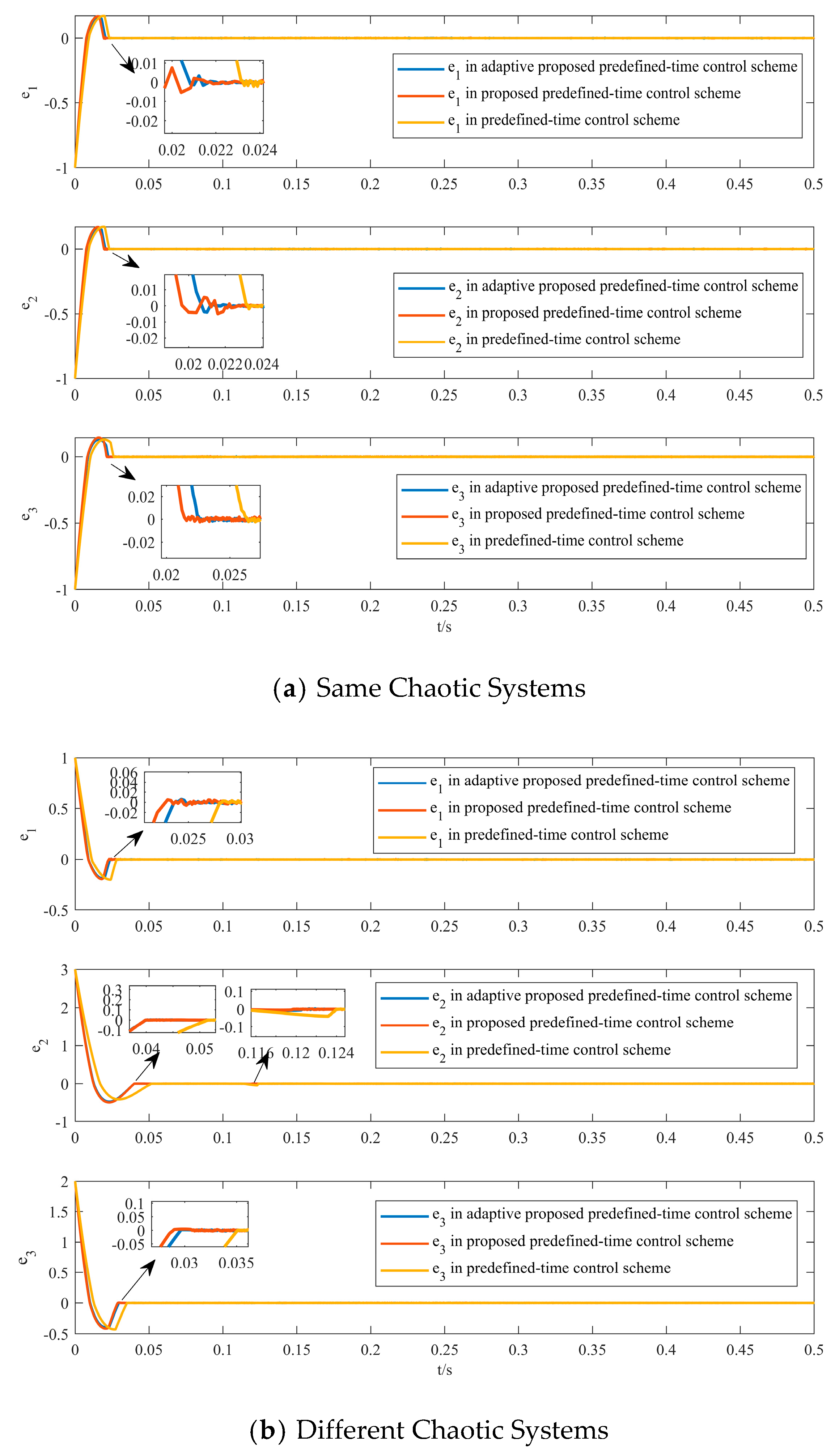
Convergence Speed of the Control Scheme.

This paper evaluates the system’s convergence speed under various predefined times through simulations, and the traditional predefined-time control scheme is compared with the fast predefined-time control scheme proposed in this paper.

(ii)

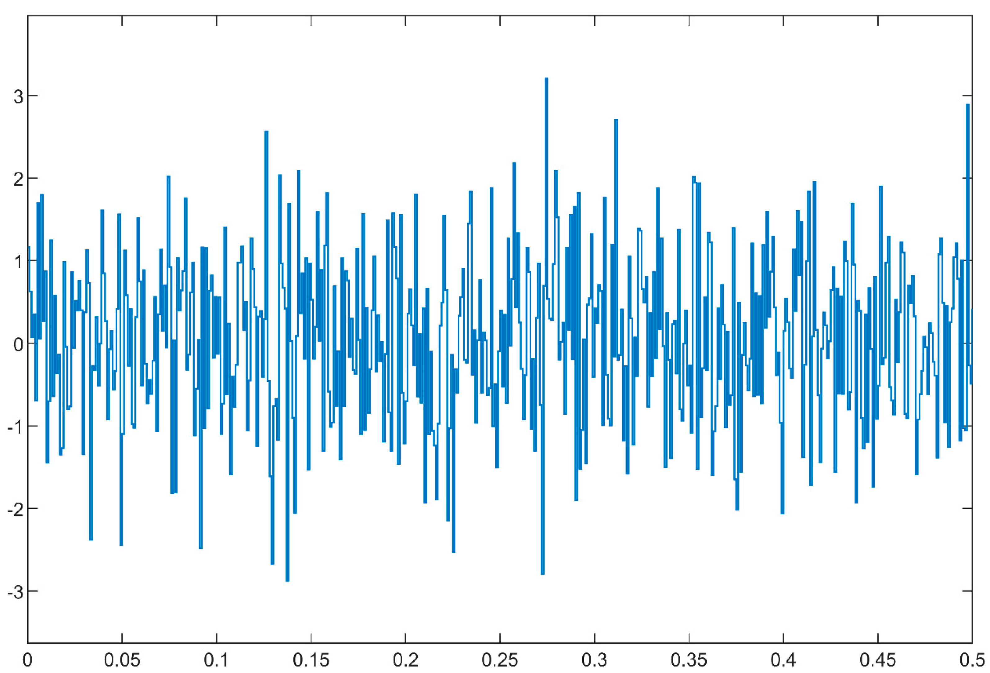
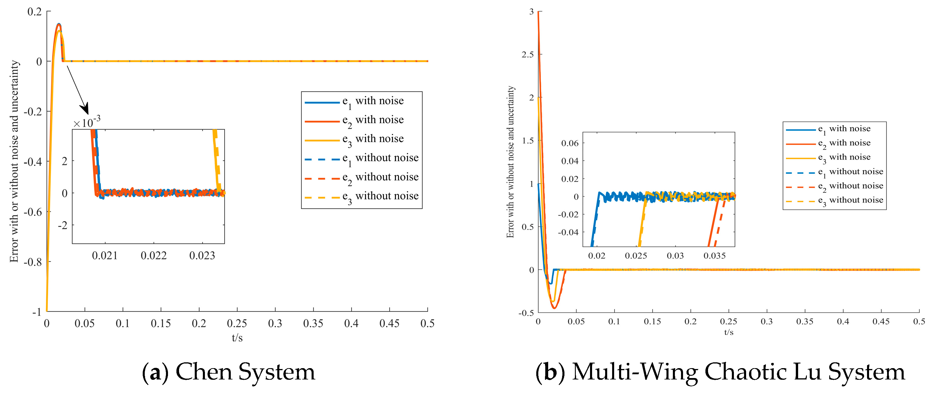
Robustness Test.

This paper compares the system’s convergence speed under different predefined times through simulations, and the traditional predefined-time control is compared with the proposed fast predefined-time control scheme.

(iii)

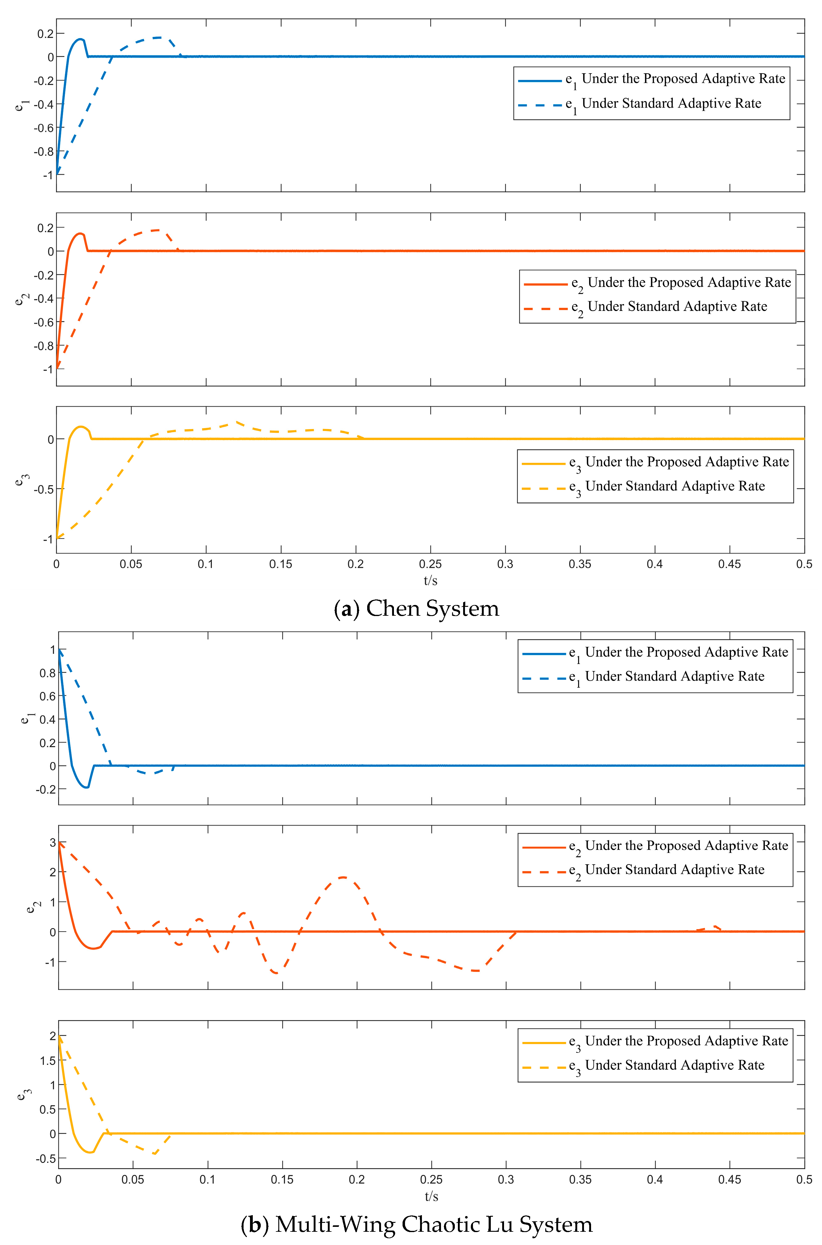
Adaptive Rate Test.

The convergence effect of the adaptive rate is evaluated by comparing the traditional adaptive rate with the norm-based adaptive rate proposed in this paper.

The state equations of the Chen system, as mentioned in reference [43], are as follows:

The drive system is represented as:

$$\left\{\begin{array}{l}{\dot{x}}_1=35(x_2-x_1)\\ {\dot{x}}_2=28x_2-x_1{x}_3-7x_1\\ {\dot{x}}_4=-3x_3+x_1{x}_2\end{array}\right.$$

(24)

The response system is represented as follows:

$$\left\{\begin{array}{l}{\dot{y}}_1=36(y_2-y_1)+u_1\\ {\dot{y}}_2=20y_2-y_1{y}_3-16y_1\\ {\dot{y}}_n=-3y_3+y_1{y}_2+u_3\end{array}\right.+u_2$$

(25)

The phase diagram of the Chen system is shown in Figure 1a.

The state equations of the multi-wing Lu system, as described in reference [44], are as follows:

The drive system is:

$$\left\{\begin{array}{l}{\dot{x}}_1=35(x_2-x_1)\\ {\dot{x}}_2=28x_2-x_1{x}_3-7x_1\\ {\dot{x}}_3=-3x_3+{2x}_1{x}_2\end{array}\right.$$

(26)

The response system is:

$$\left\{\begin{array}{l}{\dot{y}}_1=36(y_2-y_1)+u_1\\ {\dot{y}}_2=20y_2-y_1{y}_3(1-2\sin (2y_3))\\ {\dot{y}}_3=-3y_3+y_1{y}_2+u_3\end{array}\right.+u_2$$

(27)

The phase diagram of the Lu system is illustrated in Figure 1b.

For fairness of comparison, the initial state of the chaotic drive system is uniformly set to $x_1\left(0\right)=1, x_2\left(0\right)={0, x}_3\left(0\right)=3$, and the initial state of the response system is $y_1\left(0\right)=2,{ y}_2\left(0\right)=3,{ y}_3\left(0\right)=5$. The internal disturbances are selected as ${∆f}_1\left(x\right)=3\sin \left(t\right)x_1$, ${∆f}_2\left(x\right)=2\cos \left(t\right)x_2$, ${∆f}_3\left(x\right)=1.5\sin \left(t\right)x_3$, ${∆g}_1\left(y\right)=2\sin \left(t\right)y_1$, ${∆g}_2\left(y\right)=3.5\sin \left(t\right)y_2$, and ${∆g}_3\left(y\right)=4\mathrm{c}\mathrm{o}\mathrm{s}(t)y_2$. The external disturbance $d_i^m(t)=d_i^m(t)$ is a uniformly distributed random noise with an amplitude of 3.5, added to both systems in Equations (1) and (2). The values of $d_i^m(t)=d_i^m(t)$ are randomly generated within the range of 3.5, as shown in Figure 2.

4.1.1. Comparison Experiment of Different Control Schemes

Experimental Group 1: The fast predefined-time sliding mode synchronization scheme with an adaptive gain is used, where the sliding surface (7) and controllers (18), (19), and (20), along with the adaptive rate (17), are based on Theorem 2 of this paper.

Experimental Group 2: The fast predefined-time sliding mode synchronization scheme with a fixed gain is implemented, where the sliding surface (7) and controllers (18), (19), and (11) are outlined in Theorem 1 of this paper.

Control Group 1: The predefined-time sliding mode synchronization scheme is adopted, which uses the sliding surface and controller from reference [40].

To ensure the validity of the comparison experiment, similar parameter settings are uniformly applied, and based on the previously defined predefined time schemes, synchronization is set to be achieved within 1 s. The parameter settings are given by:

$$T_{{\mathrm{m}}_1}=T_{m_2}=1; p=0.5; q=2; \alpha =2; ;a_1=a_5=40; a_2=a_6={\displaystyle \frac{\pi q}{2\sqrt{3}{T}_{m}p}}$$

$$a_3=a_7={\displaystyle \frac{\pi q}{2^{1+\frac{p}{q}}\sqrt{3}{T}_{m}p}}; a_4=a_8={\displaystyle \frac{\pi q}{2^{1-\frac{p}{q}}\sqrt{3}{T}_{m}p}}; {\delta }_i=0.01;r_{i0}^{-1}=r_{i1}^{-1}=r_{i2}^{-1}=r_{i3}^{-1}=2.$$

In the Chen system (Figure 3a), significant differences are observed in the impact of the three control schemes—the adaptive control scheme, the proposed fast predefined-time control scheme, and the traditional predefined-time control scheme—on system performance. Both the proposed fast predefined-time control scheme and the adaptive fast predefined-time control scheme exhibit excellent fast response capabilities, achieving rapid error convergence to zero within $T_{max}=0.021$ s. In contrast, the traditional predefined-time control scheme demonstrates slower response speeds, with error convergence times of $T_{e_1}=T_{e_2}=0.024$ s and $T_{e_1}=0.026$ s.

The temporal differences between the control schemes are more pronounced for multi-wing chaotic Lu systems. Both the proposed fast predefined-time control scheme and the adaptive fast predefined-time control scheme achieve rapid error convergence within 0.04 s, with error convergence times of $T_{e_1}=0.024$ s, $T_{e_2}=0.04$ s, and $T_{e_3}=0.03$ s. In comparison, the original predefined-time scheme achieves convergence without steady-state error within $T_{max}=0.024$ s.

Therefore, the proposed fast predefined-time sliding mode control scheme and the adaptive fast predefined-time control scheme significantly enhance temporal control performance in identical and different chaotic systems. These schemes achieve fast error convergence and robust dynamic stability, demonstrating superior performance in reducing system errors to zero quickly in practical applications. While the traditional predefined time control scheme ensures stability, its temporal and dynamic performance is inferior to the proposed methods. These findings, validated through numerical simulations in Remarks 3 and 4, further confirm the theoretical effectiveness and superiority of the proposed control schemes.

4.1.2. Robustness Analysis

In this experiment, the sliding surface designed for the system demonstrates strong robustness in the presence of external disturbances and internal parameter uncertainties. The system still shows high robustness even without using the sgn function typically used in traditional sliding mode control schemes.

Experimental Group: The fast predefined-time sliding mode synchronization scheme with an adaptive gain is used, including the sliding surface (7), controllers (18), (19), (20), and the adaptive rate (17), as introduced in Theorem 2 of this paper.

Control Group: The sliding surface (7) is still selected, but the controller input is chosen as controllers (18) and (19).

Figure 4 presents the robustness verification of the predefined-time control scheme under different conditions, specifically, the evolution of synchronization errors in both the Chen and multi-wing chaotic Lu systems. Figure 4a,b show the error curves for identical and different chaotic systems, respectively, where the solid lines indicate the controller with specialized disturbance rejection terms. In contrast, the dashed lines indicate the absence of such terms.

The Chen system (Figure 4a): In the synchronization process of identical chaotic systems, the error curve with noise (solid line) nearly overlaps with the error curve without noise (dashed line). After $t=0.23$ s, all error variables ($e_1,{ e}_2, { e}_3$) rapidly converge to zero and reach a stable state at $t=0.24$ s. This suggests that, in identical chaotic systems, the proposed control scheme demonstrates strong robustness to noise and can effectively suppress external disturbances.

The multi-wing chaotic Lu system simulation results reveal that the error curve with noise (solid line) and the error curve without noise (dashed line) exhibit a highly consistent trend. While a slight deviation is observed in the $e_2$ error curve between 0.02 and 0.035 s, this deviation is negligible. After t = 0.035 s, all error variables ($e_1,{ e}_2, e_3$) rapidly converge to zero and reach a stable state at $t=0.36$ s, even in the presence of noise. The error curves in both cases almost completely overlap, demonstrating the proposed control scheme’s strong robustness against noise and uncertainties and its ability to ensure system stability effectively.

These results highlight the effectiveness of the proposed adaptive sliding mode control scheme, which achieves rapid error convergence and system stability under noise and uncertainties. This underscores its wide applicability and robustness in complex systems, making it particularly suitable for chaotic systems’ synchronization.

4.1.3. Comparison Experiment of Different Adaptive Rate Schemes

Experimental Group: The predefined-time sliding mode synchronization scheme with the norm-based adaptive rate proposed in this paper is implemented. The sliding surface (7), controllers (18)–(20), and adaptive rate (17) are derived from the scheme outlined in Theorem 2.

Control Group: The traditional adaptive rate in the following form is adopted. The sliding surface and controller are selected to be the same as those in the experimental group.

$$\begin{array}{l}{\dot{\tilde{l}}}_i={\dot{\widehat{l}}}_i=r_0^{-1}{s}_i(t)x_i(t)\\ {\dot{\tilde{m}}}_i={\dot{\widehat{m}}}_i=r_1^{-1}{s}_i(t)y_i(t)\\ {\dot{\tilde{D}}}_{m_i}={\dot{\widehat{D}}}_{m_i}=r_2^{-1}{s}_i(t)\\ {\dot{\tilde{D}}}_{s_i}={\dot{\widehat{D}}}_{s_i}=r_3^{-1}{s}_i(t)\end{array}$$

(28)

The results are shown in Figure 5.

Figure 5a compares the synchronization performance between two adaptive rates under the Chen chaotic system. The error curves indicate that the norm-based adaptive rate enables system errors $e_1, e_2, e_3$ to rapidly converge to zero within 0.05 s, exhibiting smooth trajectories without noticeable oscillations or fluctuations. In contrast, the standard adaptive rate shows slower convergence, particularly for $e_2$, which experiences larger fluctuations and only stabilizes around 0.2 s. Furthermore, the standard adaptive rate error curves display significant oscillations during the convergence process, underscoring its weaker dynamic performance. In comparison, the proposed norm-based adaptive rate demonstrates superior adaptability and enhanced dynamic adjustment capabilities, making it more effective for synchronization across different chaotic systems.

Figure 5b compares the performance of the norm-based and standard adaptive rates under the multi-wing Lu chaotic system. The norm-based adaptive rate achieves rapid convergence with $e_1, e_2, e_3$ stabilizing near zero within 0.05 s. The error curves associated with the norm-based adaptive rate are smooth and exhibit no significant fluctuations, demonstrating its stability. In contrast, the standard adaptive rate shows slower convergence, particularly for $e_2$, which exhibits the largest fluctuations and only stabilizes around 0.45 s. Additionally, the error curves of the standard adaptive rate reveal noticeable oscillations during the convergence process, highlighting its weaker dynamic performance. The proposed norm-based adaptive rate demonstrates superior adaptability and enhanced dynamic adjustment capabilities.

Therefore, the adaptive rate proposed in this paper demonstrates significant advantages in identical and different chaotic systems. It achieves fast and stable error convergence to zero while avoiding the oscillations and instability observed with traditional adaptive rates. These findings indicate that the proposed adaptive rate scheme offers superior performance and high practical value in controlling chaotic systems. Furthermore, this conclusion aligns with the theoretical analysis presented in Remark 6, as numerical simulation experiments validate the effectiveness and robustness of the improved adaptive rate scheme in practical applications.

4.2. Actual Chaotic System Experiment (Memristor Experiment)

In this experiment, the memristor model from reference [45] was selected to represent the actual chaotic system. The primary objective was to evaluate the performance of the proposed control scheme in this real-world chaotic system. The parameters and initial conditions of the memristor were set according to reference [45], while the controller parameters were configured as outlined in Section 4.1.1, “Comparison Experiment of Different Control Schemes”.

Figure 6 compares the memristor chaotic synchronization under three different control schemes: the adaptive proposed predefined-time control scheme (blue line), the proposed predefined-time control scheme (red line), and the standard predefined-time control scheme (yellow line). Both the adaptive proposed control scheme (blue line) and the proposed predefined-time control scheme (red line) show fast convergence, with all four state errors converging within approximately 0.05 s for the blue line and 0.07 s for the red line. In contrast, the yellow line (standard predefined-time control scheme) exhibits slower convergence, with all errors converging within 0.17 s. Notably, the adaptive proposed control scheme (blue line) and the proposed predefined-time control scheme (red line) show significantly faster convergence for $e_1$ and $e_3$ compared with the yellow line (standard predefined-time control scheme). These results highlight the superior performance of the proposed control schemes, with the adaptive scheme offering the fastest synchronization and best error suppression.

These findings indicate that the proposed adaptive rate scheme offers superior performance and high practical value in controlling chaotic systems. Moreover, this approach is not limited to the memristor chaotic synchronization system and can be extended to other applications, such as PMSM chaotic synchronization, demonstrating its broad applicability in solving practical engineering problems.

5. Conclusions

This paper presents an adaptive predefined-time sliding mode control method for synchronizing chaotic systems under external disturbances and modeling uncertainties. The theoretical analysis rigorously demonstrates that the proposed control scheme ensures predefined time stability by constructing a Lyapunov function. Additionally, the norm-based adaptive rate dynamically adjusts the control gain to effectively counteract external disturbances, achieving fast convergence and zero synchronization error within a predefined time.

The effectiveness and superiority of the proposed method were validated through numerical simulations involving identical and different chaotic systems, including the Chen system and the multi-wing chaotic Lu system. The simulation results indicate that the proposed fast predefined-time control scheme and its adaptive variant significantly outperform traditional methods regarding convergence speed, dynamic stability, and robustness. In particular, the adaptive predefined-time scheme exhibited strong noise immunity and the capability to handle uncertainties effectively, ensuring high precision and reliability in chaotic system synchronization.

Moreover, the proposed control scheme is highly versatile and can be extended to fractional-order chaotic systems, offering broader applicability. This approach could also be adapted to a wide range of practical scenarios, including UAV control, underwater vehicle control, communication encryption, and other fields where rapid and reliable synchronization is crucial. Its robustness and adaptability make it a promising solution for complex, real-world systems.

References

- Pecora, L.M.; Carroll, T.L. Synchronization in chaotic systems. J. Nonlinear Sci. 1990, 64, 821. [Google Scholar] [CrossRef]
- Chen, Y.-J.; Chou, H.-G.; Wang, W.-J.; Tsai, S.-H.; Tanaka, K.; Wang, H.O.; Wang, K.C. A polynomial-fuzzy-model-based synchronization methodology for the multi-scroll Chen chaotic secure communication system. Eng. Appl. Artif. Intell. 2020, 87, 103251. [Google Scholar] [CrossRef]
- Hamidzadeh, S.M.; Rezaei, M.; Ranjbar-Bourani, M. Chaos synchronization for a class of uncertain chaotic supply chain and its control by ANFIS. Int. J. Prod. Manag. Eng. 2023, 11, 113–126. [Google Scholar] [CrossRef]
- Aliabadi, F.; Majidi, M.-H.; Khorashadizadeh, S. Chaos synchronization using adaptive quantum neural networks and its application in secure communication and cryptography. Neural Comput. Appl. 2022, 34, 6521–6533. [Google Scholar] [CrossRef]
- Lawnik, M.; Berezowski, M. New chaotic system: M-map and its application in chaos-based cryptography. Symmetry 2022, 14, 895. [Google Scholar] [CrossRef]
- Liu, Y. Circuit implementation and finite-time synchronization of the 4D Rabinovich hyperchaotic system. Nonlinear Dyn. 2012, 67, 89–96. [Google Scholar] [CrossRef]
- Tian, K.; Grebogi, C.; Ren, H.-P. Chaos generation with impulse control: Application to non-chaotic systems and circuit design. IEEE Trans. Circuits Syst. I Regul. Pap. 2021, 68, 3012–3022. [Google Scholar] [CrossRef]
- Gong, L.-H.; Luo, H.-X.; Wu, R.-Q.; Zhou, N.-R. New 4D chaotic system with hidden attractors and self-excited attractors and its application in image encryption based on RNG. Phys. A Stat. Mech. Its Appl. 2022, 591, 126793. [Google Scholar] [CrossRef]
- Spitz, O.; Herdt, A.; Wu, J.; Maisons, G.; Carras, M.; Wong, C.-W.; Elsäßer, W.; Grillot, F. Private communication with quantum cascade laser photonic chaos. Nat. Commun. 2021, 12, 3327. [Google Scholar] [CrossRef]
- Xiao, Y.; Xu, W.; Li, X.; Tang, S. Adaptive complete synchronization of chaotic dynamical network with unknown and mismatched parameters. Chaos Interdiscip. J. Nonlinear Sci. 2007, 17, 033118. [Google Scholar] [CrossRef]
- Guan, S.; Lai, C.-H.; Wei, G.-W. Phase synchronization between two essentially different chaotic systems. Phys. Rev. E 2005, 72, 016205. [Google Scholar] [CrossRef] [PubMed]
- Femat, R.; Solís-Perales, G. Synchronization of chaotic systems with different order. Phys. Rev. E 2002, 65, 036226. [Google Scholar] [CrossRef] [PubMed]
- Zhou, Q.; Zhao, S.; Li, H.; Lu, R.; Wu, C. Adaptive neural network tracking control for robotic manipulators with dead zone. IEEE Trans. Neural Netw. Learn. Syst. 2018, 30, 3611–3620. [Google Scholar] [CrossRef] [PubMed]
- Pal, P.; Jin, G.G.; Bhakta, S.; Mukherjee, V. Adaptive chaos synchronization of an attitude control of satellite: A backstepping based sliding mode approach. Heliyon 2022, 8, e11730. [Google Scholar] [CrossRef]
- Xu, Y.; Yu, J.; Li, W.; Feng, J. Global asymptotic stability of fractional-order competitive neural networks with multiple time-varying-delay links. Appl. Math. Comput. 2021, 389, 125498. [Google Scholar] [CrossRef]
- Deepika, D. Hyperbolic uncertainty estimator based fractional order sliding mode control framework for uncertain fractional order chaos stabilization and synchronization. ISA Trans. 2022, 123, 76–86. [Google Scholar] [CrossRef] [PubMed]
- Anguiano-Gijón, C.A.; Muñoz-Vázquez, A.J.; Sánchez-Torres, J.D.; Romero-Galván, G.; Martínez-Reyes, F. On predefined-time synchronisation of chaotic systems. Chaos Solitons Fractals 2019, 122, 172–178. [Google Scholar] [CrossRef]
- Song, J.; Niu, Y.; Zou, Y. Finite-time stabilization via sliding mode control. IEEE Trans. Autom. Control 2016, 62, 1478–1483. [Google Scholar] [CrossRef]
- Wang, L.; Dong, T.; Ge, M.-F. Finite-time synchronization of memristor chaotic systems and its application in image encryption. Appl. Math. Comput. 2019, 347, 293–305. [Google Scholar] [CrossRef]
- Ni, J.; Liu, L.; Liu, C.; Hu, X. Fractional order fixed-time nonsingular terminal sliding mode synchronization and control of fractional order chaotic systems. Nonlinear Dyn. 2017, 89, 2065–2083. [Google Scholar] [CrossRef]
- Shirkavand, M.; Pourgholi, M. Robust fixed-time synchronization of fractional order chaotic using free chattering nonsingular adaptive fractional sliding mode controller design. Chaos Solitons Fractals 2018, 113, 135–147. [Google Scholar] [CrossRef]
- Jiménez-Rodríguez, E.; Sánchez-Torres, J.D.; Loukianov, A.G. On optimal predefined-time stabilization. Int. J. Robust Nonlinear Control 2017, 27, 3620–3642. [Google Scholar] [CrossRef]
- Assali, E.A. Predefined-time synchronization of chaotic systems with different dimensions and applications. Chaos Solitons Fractals 2021, 147, 110988. [Google Scholar] [CrossRef]
- Li, Q.; Yue, C. Predefined-time polynomial-function-based synchronization of chaotic systems via a novel sliding mode control. IEEE Access 2020, 8, 162149–162162. [Google Scholar] [CrossRef]
- Xie, S.; Chen, Q. Adaptive nonsingular predefined-time control for attitude stabilization of rigid spacecrafts. IEEE Trans. Circuits Syst. II Express Briefs 2021, 69, 189–193. [Google Scholar] [CrossRef]
- Vaidyanathan, S. Adaptive control of a chemical chaotic reactor. Int. J. PharmTech Res. 2015, 8, 377–382. [Google Scholar]
- Vaseghi, B.; Pourmina, M.A.; Mobayen, S. Secure communication in wireless sensor networks based on chaos synchronization using adaptive sliding mode control. Nonlinear Dyn. 2017, 89, 1689–1704. [Google Scholar] [CrossRef]
- Khan, A.; Kumar, S. Measuring chaos and synchronization of chaotic satellite systems using sliding mode control. Optim. Control Appl. Methods 2018, 39, 1597–1609. [Google Scholar] [CrossRef]
- Fei, J.; Feng, Z. Fractional-order finite-time super-twisting sliding mode control of micro gyroscope based on double-loop fuzzy neural network. IEEE Trans. Syst. Man Cybern. Syst. 2020, 51, 7692–7706. [Google Scholar] [CrossRef]
- Cao, Y.; Chen, X. An output-tracking-based discrete PID-sliding mode control for MIMO systems. IEEE/ASME Trans. Mechatron. 2013, 19, 1183–1194. [Google Scholar] [CrossRef]
- Modiri, A.; Mobayen, S. Adaptive terminal sliding mode control scheme for synchronization of fractional-order uncertain chaotic systems. ISA Trans. 2020, 105, 33–50. [Google Scholar] [CrossRef]
- Zhang, M.; Zang, H.; Bai, L. A new predefined-time sliding mode control scheme for synchronizing chaotic systems. Chaos Solitons Fractals 2022, 164, 112745. [Google Scholar] [CrossRef]
- Dadras, S.; Dadras, S.; Momeni, H. Linear matrix inequality based fractional integral sliding-mode control of uncertain fractional-order nonlinear systems. J. Dyn. Syst. Meas. Control 2017, 139, 111003. [Google Scholar] [CrossRef]
- Deepika, D.; Kaur, S.; Narayan, S. Uncertainty and disturbance estimator based robust synchronization for a class of uncertain fractional chaotic system via fractional order sliding mode control. Chaos Solitons Fractals 2018, 115, 196–203. [Google Scholar] [CrossRef]
- Saeed, N.A.; Saleh, H.A.; El-Ganaini, W.A.; Kamel, M.; Mohamed, M.S. On a New Three-Dimensional Chaotic System with Adaptive Control and Chaos Synchronization. Shock. Vib. 2023, 2023, 1969500. [Google Scholar] [CrossRef]
- Ahmad, I.; Shafiq, M. Robust adaptive anti-synchronization control of multiple uncertain chaotic systems of different orders. Automatika 2020, 61, 396–414. [Google Scholar] [CrossRef]
- Alimi, M.; Rhif, A.; Rebai, A.; Vaidyanathan, S.; Azar, A.T. Optimal adaptive backstepping control for chaos synchronization of nonlinear dynamical systems. In Backstepping Control of Nonlinear Dynamical Systems; Elsevier: Amsterdam, The Netherlands, 2021; pp. 291–345. [Google Scholar]
- Kobiolka, J.; Habermann, J.; Yamakou, M.E. Reduced-order adaptive synchronization in a chaotic neural network with parameter mismatch: A dynamical system vs. machine learning approach. arXiv 2024, arXiv:2408.16155. [Google Scholar]
- Wang, S. A novel memristive chaotic system and its adaptive sliding mode synchronization. Chaos Solitons Fractals 2023, 172, 113533. [Google Scholar] [CrossRef]
- Roldán-Caballero, A.; Pérez-Cruz, J.H.; Hernández-Márquez, E.; García-Sánchez, J.R.; Ponce-Silva, M.; Rubio, J.d.J.; Villarreal-Cervantes, M.G.; Martínez-Martínez, J.; García-Trinidad, E.; Mendoza-Chegue, A. Synchronization of a new chaotic system using adaptive control: Design and experimental implementation. Complexity 2023, 2023, 2881192. [Google Scholar] [CrossRef]
- Keighobadi, J.; Hosseini-Pishrobat, M.; Faraji, J. Adaptive neural dynamic surface control of mechanical systems using integral terminal sliding mode. Neurocomputing 2020, 379, 141–151. [Google Scholar] [CrossRef]
- Fathollahi, A.; Andresen, B. Adaptive Fixed-Time Control strategy of Generator Excitation and Thyristor-Controlled Series Capacitor in Multi-Machine Energy Systems. IEEE Access 2024, 12, 100316–100327. [Google Scholar] [CrossRef]
- Tian, K.; Ren, H.-P.; Grebogi, C. Existence of chaos in the Chen system with linear time-delay feedback. Int. J. Bifurc. Chaos 2019, 29, 1950114. [Google Scholar] [CrossRef]
- Sahoo, S.; Roy, B.K. Design of multi-wing chaotic systems with higher largest Lyapunov exponent. Chaos Solitons Fractals 2022, 157, 111926. [Google Scholar] [CrossRef]
- Wang, Y.; Li, H.; Guan, Y.; Chen, M. Predefined-time chaos synchronization of memristor chaotic systems by using simplified control inputs. Chaos Solitons Fractals 2022, 161, 112282. [Google Scholar] [CrossRef]
Disclaimer/Publisher’s Note: The statements, opinions and data contained in all publications are solely those of the individual author(s) and contributor(s) and not of MDPI and/or the editor(s). MDPI and/or the editor(s) disclaim responsibility for any injury to people or property resulting from any ideas, methods, instructions or products referred to in the content. |
© 2025 by the authors. Licensee MDPI, Basel, Switzerland. This article is an open access article distributed under the terms and conditions of the Creative Commons Attribution (CC BY) license (https://creativecommons.org/licenses/by/4.0/).
Share and Cite
Ding, H.; Qian, J.; Tian, D.; Zeng, Y. Norm-Based Adaptive Control with a Novel Practical Predefined-Time Sliding Mode for Chaotic System Synchronization. Mathematics 2025, 13, 748. https://doi.org/10.3390/math13050748
Ding H, Qian J, Tian D, Zeng Y. Norm-Based Adaptive Control with a Novel Practical Predefined-Time Sliding Mode for Chaotic System Synchronization. Mathematics. 2025; 13(5):748. https://doi.org/10.3390/math13050748
Chicago/Turabian StyleDing, Huan, Jing Qian, Danning Tian, and Yun Zeng. 2025. "Norm-Based Adaptive Control with a Novel Practical Predefined-Time Sliding Mode for Chaotic System Synchronization" Mathematics 13, no. 5: 748. https://doi.org/10.3390/math13050748
APA StyleDing, H., Qian, J., Tian, D., & Zeng, Y. (2025). Norm-Based Adaptive Control with a Novel Practical Predefined-Time Sliding Mode for Chaotic System Synchronization. Mathematics, 13(5), 748. https://doi.org/10.3390/math13050748