Synchronization in Fractional-Order Delayed Non-Autonomous Neural Networks

Abstract

Neural networks, mimicking the structural and functional aspects of the human brain, have found widespread applications in diverse fields such as pattern recognition, control systems, and information processing. A critical phenomenon in these systems is synchronization, where multiple neurons or neural networks harmonize their dynamic behaviors to a common rhythm, contributing significantly to their efficient operation. However, the inherent complexity and nonlinearity of neural networks pose significant challenges in understanding and controlling this synchronization process. In this paper, we focus on the synchronization of a class of fractional-order, delayed, and non-autonomous neural networks. Fractional-order dynamics, characterized by their ability to capture memory effects and non-local interactions, introduce additional layers of complexity to the synchronization problem. Time delays, which are ubiquitous in real-world systems, further complicate the analysis by introducing temporal asynchrony among the neurons. To address these challenges, we propose a straightforward yet powerful global synchronization framework. Our approach leverages novel state feedback control to derive an analytical formula for the synchronization controller. This controller is designed to adjust the states of the neural networks in such a way that they converge to a common trajectory, achieving synchronization. To establish the asymptotic stability of the error system, which measures the deviation between the states of the neural networks, we construct a Lyapunov function. This function provides a scalar measure of the system’s energy, and by showing that this measure decreases over time, we demonstrate the stability of the synchronized state. Our analysis yields sufficient conditions that guarantee global synchronization in fractional-order neural networks with time delays and Caputo derivatives. These conditions provide a clear roadmap for designing neural networks that exhibit robust and stable synchronization properties. To validate our theoretical findings, we present numerical simulations that demonstrate the effectiveness of our proposed approach. The simulations show that, under the derived conditions, the neural networks successfully synchronize, confirming the practical applicability of our framework.

1. Introduction

In practical neural network models, external influences and internal system dynamics can degrade system stability, potentially leading to instability. When selecting a fractional-order neural network as a research subject, it is crucial to account for these effects and focus on analyzing its stability, as well as devising a simple and effective synchronous controller. Only by addressing these aspects can we effectively utilize fractional-order neural networks and enhance their practical applications. Synchronization, a prevalent dynamic behavior in real-world systems, underscores the importance of studying synchronization in fractional-order neural network models. Consequently, numerous scholars have dedicated their research to this topic, as evidenced in [1,2,3,4,5,6,7] and related references.

In 2014, Yu et al. [8] conducted research on the global projective synchronization of a specific fractional-order neural network model:

$$D^{\alpha }{x}_i(t)=-a_i{x}_i(t)+{\displaystyle \sum _{j=1}^n{c}_{ij}{f}_j(x_j(t))+}{I}_i,\hspace{0.33em}{x}_i(t_0)=x_{0i},\hspace{0.33em}i=1,2,\cdots ,n.$$

(1)

where $0<\alpha <1$. Utilizing certain analytical techniques and integrating open-loop and adaptive control methods, Yu et al. derived novel criteria that ensure the projection synchronization of fractional-order neural networks. In 2018, Hu et al. [9] delved into the global asymptotic synchronization issue of the aforementioned fractional-order neural network model (1). Initially, they explored fresh properties of fractional calculus and formulated the asymptotic stability theorem for fractional-order systems represented by (1). Furthermore, they introduced a novel feedback controller. Ultimately, by leveraging the proposed asymptotic stability theorem and matrix inequality techniques, they established sufficient conditions for achieving global asymptotic synchronization in fractional-order neural networks. However, it is evident that Model (1) lacks a delay term. In reality, time delays are ubiquitous in numerous network domains. Considering fluctuations in network parameters due to hardware operations and the limited switching speeds of signal transmitters and amplifiers within the network, incorporating delays into neural network systems is imperative. Consequently, in recent times, the investigation of dynamic behaviors in delayed fractional-order neural networks (DFNNs) has garnered increasing attention from scholars. For instance, in 2015, Wang et al. [10] conducted a study on the fractional-order Hopfield neural network incorporating time delays:

$$D_t^q{x}_i(t)=-a_i{x}_i(t)+{\displaystyle {\sum }_{j=1}^n{b}_{ij}{f}_j(x_j(t))}+{\displaystyle {\sum }_{j=1}^n{c}_{ij}{g}_j(x_j(t-{\tau }_{ij}))},\hspace{0.33em}t>0,\hspace{0.33em}i=1,2,\cdots ,n,$$

(2)

where $q\in (0,1),$$a_i,b_{ij},c_{ij}$ are constants. Utilizing the linearization method and Laplace transform, they derived stability conditions for two-dimensional fractional-order neural networks with time delays. Additionally, they proposed three-dimensional fractional-order neural networks featuring diverse ring structures and time delays, along with the corresponding stability conditions for these networks. In 2017, Peng et al. [11] investigated fractional-order neural networks that incorporate discontinuous activations and time delays:

$${}_t{}^{c}D_0^{\alpha }x(t)=-Cx(t)+Af(x(t))+Bf(x(t-\tau ))+I$$

(3)

where $x(t)={(x_1(t),x_2(t),\cdots ,x_n(t))}^T\in R^n$ is the vector of neuron states at time $t$. By applying the fractional differential inclusion theory, inequality analysis techniques, and linear matrix inequalities, Peng et al. provided sufficient conditions to ensure global Mittag–Leffler synchronization and finite-time synchronization. In 2018, Zhang et al. [12] examined the drive–response synchronization problem for a specific class of fractional-order delay neural networks. The model in question is as follows:

$$D^{\alpha }{x}_i(t)=-c_i{x}_i(t)+{\displaystyle \sum _{j=1}^n{a}_{ij}{f}_j(x_j(t))+}{\displaystyle \sum _{j=1}^n{b}_{ij}{f}_j(x_j(t-\tau ))}+I_i,$$

(4)

where $0<\alpha <1,i\in N=1,2,\cdots ,n.$ Both a state feedback controller and an adaptive controller were designed, and several novel synchronization conditions were derived utilizing relevant theoretical knowledge to guarantee the global synchronization of System (4).

On the other hand, it is generally recognized that obtaining exact values for model parameters is often impractical. This is primarily due to inherent perturbations in the model and environmental disturbances, which result in parameter uncertainty. Consequently, when analyzing the dynamic behavior of nonlinear systems, the impact of these parameter uncertainties cannot be overlooked, as they may compromise the stability, synchronization, or other properties of the system. In recent years, numerous studies have centered on the synchronization of neural network models with parametric uncertainty. In 2018, researchers [13] explored the synchronization problem in delayed fractional-order complex-valued neural networks with memristors and uncertain parameters. They derived sufficient conditions to ensure global asymptotic synchronization for the drive–response models in question, utilizing the differential inclusion theory, Lyapunov direct method, and comparison theorem. It is particularly noteworthy that Wang et al. [14] conducted a study on the following non-autonomous fractional-order delayed neural network:

$$D^{\alpha }{x}_i(t)=e^{pt}\left[-a_i{x}_i(t)+{\displaystyle \sum _{j=1}^n{b}_{ij}}{f}_j(x_j(t))+{\displaystyle \sum _{j=1}^n{c}_{ij}{f}_j}(x_j(t-\tau ))\right]+I_i,\hspace{0.33em}i=1,2,\cdots ,n.$$

(5)

Utilizing the Mittag–Leffler function and linear feedback control, Wang et al. derived the analytic expression for the synchronization controller. Furthermore, they obtained a sufficient condition to guarantee the synchronization of this delayed fractional-order neural network with Caputo derivatives. This was achieved by developing innovative analysis methods, employing the theory of delayed differential inequalities, and constructing an appropriate Lyapunov function. In 2024, Wang et al. [15] continued their research on the following non-autonomous neural networks, incorporating time delays and Caputo derivatives:

$$D^{\alpha }{u}_i(t)=e^{pt}\left[-a_i{u}_i(t)+{\displaystyle \sum _{j=1}^n{b}_{ij}}{g}_j(u_j(t))+{\displaystyle \sum _{j=1}^n{c}_{ij}{f}_j}(u_j(t-\tau ))\right]+I_i,\hspace{0.33em}i=1,2,\cdots ,n.$$

(6)

By constructing two innovative Lyapunov functions and leveraging the properties of fractional-order delay differential inequalities, Wang et al. derived criteria for achieving global projective synchronization in delayed non-autonomous neural networks with Caputo derivatives. These criteria were obtained under the conditions of two newly proposed synchronous controllers.

However, to our knowledge, previous research has seldom explored non-autonomous delayed fractional-order neural networks (DFNNs). These networks can more accurately simulate the interactions between neurons, as the connection weights and self-inhibition rates within neural networks are typically not constant but rather functions that vary over time. Motivated by prior studies, the aim of this paper is to investigate the global synchronization of a broader class of non-autonomous DFNNs incorporating the Caputo derivative. By constructing a Lyapunov function, we verify the asymptotic stability of the error system and derive sufficient conditions for ensuring global synchronization in these new neural networks. The structure of this paper is as follows: Section 2 introduces necessary definitions and lemmas, along with a description of the model. In Section 3, we obtain global synchronization schemes and provide sufficient conditions for global synchronization in the new neural networks. Section 4 presents numerical simulations to validate our findings. Finally, Section 5 concludes this paper with some remarks.

2. Preliminaries and System Description

In this paper, $R$ represents a real space, while $R^m$ denotes an m-dimensional Euclidean space. $N^{+}$ is a set consisting of positive integers. The gamma functions $\Gamma (z)$, $E_{\alpha }(\cdot )$, and $E_{\alpha ,\beta }(\cdot )$ are defined as follows:

Definition 1 ([16,17]).

The fractional integral of the integrable function $x(t)$ is defined as:

$$D_{t_0}^{-\alpha }x(t)={\displaystyle \frac{1}{\Gamma (\alpha )}}{\displaystyle {\int }_{t_0}^t{(t-s)}^{\alpha -1}x(s)ds},$$

(7)

where $t\ge t_0$, order $\alpha >0$. $\Gamma (\cdot )$ is a gamma function, which is defined as:

$$\Gamma (\alpha )={\displaystyle {\int }_0^{\infty }{e}^{-t}{t}^{\alpha -1}}dt,$$

(8)

satisfying the recursive relationship $\Gamma (\alpha +1)=\alpha \Gamma (\alpha )$.

Definition 2.

The single-parameter Mittag–Leffler function is defined as follows:

Given $\alpha >0,z\in C$, we denote 

$$E_{\alpha }(z)={\displaystyle \sum _{k=0}^{\infty }\frac{z^k}{\Gamma (k\alpha +1)}}$$

(9)

as the single-parameter Mittag–Leffler function.

Definition 3.

The two-parameter Mittag–Leffler function is defined as follows:

Given $\alpha >0,\beta >0$ and $z\in C$, we denote 

$$E_{\alpha ,\beta }(z)={\displaystyle \sum _{k=0}^{\infty }\frac{z^k}{\Gamma (k\alpha +\beta )}}$$

(10)

as the two-parameter Mittag–Leffler function.

Based on the above definitions, it holds that $E_{\alpha }(z)=E_{\alpha ,1}(z),E_{1,1}(z)=e^z$.

As mentioned above, in physical systems, the Caputo fractional derivative carries more practical physical meaning and is more suitable for describing actual systems with initial values compared to the Riemann–Liouville (RL) fractional derivative and the Grünwald–Letnikov (GL) fractional derivative. Consequently, in practical applications, the Caputo differential operation is more frequently utilized than the RL and GL differential operations. Therefore, the definition of the Caputo fractional derivative will also be employed in this article.

Definition 4 ([16,17]).

The Caputo fractional derivative of function $x(t)$ is defined as: 

$$D_{t_0}^{\alpha }x(t)={\displaystyle \frac{1}{\Gamma (n-\alpha )}}{{\displaystyle {\int }_{t_0}^t(t-s)}}^{n-\alpha -1}{\left({\displaystyle \frac{d}{ds}}\right)}^{n}x(s)ds,$$

(11)

where $\alpha$ represents the order of the derivative, $n-1<\alpha \le n.$

In particular, when $0<\alpha <1$, the following applies:

$$D^{\alpha }x(t)={\displaystyle \frac{1}{\Gamma (1-\alpha )}}{{\displaystyle {\int }_{t_0}^t(t-s)}}^{-\alpha }{x}^{\prime }(s)ds.$$

(12)

Lemma 1 ([17]).

For any constant $c_1,c_2,$ if $w(t),u(t)\in [t_0,b], \alpha >0,\beta >0,$ then

(1)  $D^{\alpha }{D}^{-\beta }w(t)=D^{\alpha -\beta }w(t),$

(2)  $D^{-\alpha }{D}^{\alpha }w(t)=w(t),$

(3)  $D^{\alpha }(c_{1}w(t)\pm c_{2}u(t))=c_1{D}^{\alpha }w(t)\pm c_2{D}^{\alpha }u(t).$

Lemma 2 ([18]).

Assume that $f(t)\in R^n$ is a differentiable vector value function and $P\in R^{n\times n}$ is a positive definite, symmetric matrix. Then, it holds that 

$$D^{\alpha }(f^T(s)Pf(s))\le 2f^T(s)P{D}^{\alpha }f(s),$$

(13)

where $\alpha \in [0,1], s\ge s_0$.

Lemma 3 ([19]).

Consider a Captuto fractional differential system $D^{\alpha }x(t)=f(t,x(t),x(t-\tau ))$, where $x\in R^n$, $0<\alpha <1$. Suppose that $w_1(s),w_2(s)$ are continuous non-decreasing functions, $w_1(s)$ and $w_2(s)$ are positive for $s>0$, $w_1(0)=w_2(0)$, and $w_2(s)$ is strictly increasing. If there exists a continuously differentiable function $V:R\times R^n\to R$ such that $w_1(‖x‖)\le V(t,x)\le w_2(‖x‖)$, for $t\in R$, $x\in R^n,$ and additionally, if there are two positive constants $p$ and $q$, such that $p<q$ and 

$$D^{\alpha }V(t,x(t))\le -qV(t,x(t))+p\underset{-\tau \le \theta \le 0}{\sup }V(t+\theta ,x(t+\theta )),\hspace{0.33em}t\ge t_0,$$

(14)

then the Caputo fractional system is globally uniformly asymptotically stable.

In this article, we investigate non-autonomous neural networks with time delays and the Caputo derivative serving as the leader system. This system is characterized by the following:

$$D^{\alpha }{x}_i(t)=-c_i(t)x_i(t)+{\displaystyle \sum _{j=1}^n{a}_{ij}}(t)f_j(x_j(t))+{\displaystyle \sum _{j=1}^n{b}_{ij}(t)}{g}_j(x_j(t-\tau ))+I_i.$$

(15)

Alternatively, they can be expressed in vector form:

$$D^{\alpha }x(t)=-C(t)x(t)+A(t)f(x(t))+B(t)g(x(t-\tau ))+I,$$

(16)

where each element in $C(t)$ is required to be a positive bounded function, and each element in $A(t),B(t)$ is a bounded function. $0<\alpha <1,$$i\in N=1,2,\cdots ,n,t\ge 0,\hspace{0.33em}n$ represents the number of neurons, $x(t)=(x_1(t)),\cdots ,x_n(t){)}^T\in R^n$ represents a state variable at time $t$,$\tau$ represents the propagation delay of the neuron,$x(t-\tau )=(x_1(t-\tau )),\cdots ,x_n(t-\tau ){)}^T\in R^n$ represent a state variable at time $t-\tau$, and $f(x(t))={(f_1(x_1(t)),\cdots ,f_n(x_n(t)))}^T$ and $g(x(t))={(g_1(x_1(t)),\cdots ,g_n(x_n(t)))}^T$ $(n\in N^{+})$ denote the excitation function of a neuron at time $t$ and $t-\tau$, respectively. $C(t)$ denotes a self-joining weight of a neuron, $A(t)$ denotes an internal connection weight matrix when there is no time delay, $B(t)$ denotes an internal connection weight matrix when there is a time delay, and $I={(I_1,I_2\cdots ,I_n)}^T$ denotes an external input vector. Neural network models (15) can be employed to simulate the analysis and processing of diverse types of information performed by the human brain. They constitute a crucial element of artificial intelligence algorithms.

3. Main Conclusions and Their Proof

Consider the follower system of leader system (15), which is characterized as follows:

$$D^{\alpha }{y}_i(t)=-c_i(t)y_i(t)+{\displaystyle \sum _{j=1}^n{a}_{ij}}(t)f_j(y_j(t))+{\displaystyle \sum _{j=1}^n{b}_{ij}(t)}{g}_j(y_j(t-\tau ))+I_i+u_i(t).$$

(17)

Alternatively, they can be expressed in vector form:

$$D^{\alpha }y(t)=-C(t)y(t)+A(t)f(y(t))+B(t)g(y(t-\tau ))+I+u(t),$$

(18)

where $y(t)=(y_1(t)),\cdots ,y_n(t){)}^T\in R^n$ represents a state variable from the follower system (18), $u(t)={(u_1(t),\cdots ,u_n(t))}^T$ represents the synchronous controller of the follower system (18), and the representation of $A(t),B(t),C(t),$$f(\cdot ),$$g(\cdot )$ is consistent with the leader system (17).

We define the synchronous error vector as $e_i(t)=y_i(t)-x_i(t)(i=1,2,\cdots ,n)$. Then, using the leader system (15) and the follower system (17), we can derive the expression for the error system, which is given as follows:

$$\begin{array}{cc}\hfill D^{\alpha }{e}_i(t)=& -c_i(t)e_i(t)+{\displaystyle \sum _{j=1}^n{a}_{ij}}(t)[f_j(y_j(t))-f_j(x_j(t))]\hfill \\ & +{\displaystyle \sum _{j=1}^n{b}_{ij}(t)}[g_j(y_j(t-\tau ))-g_j(x_j(t-\tau ))]+u_i(t),\hfill \end{array}$$

(19)

Alternatively, they can be expressed in vector form:

$$D^{\alpha }e(t)=-C(t)e(t)+A(t)[f(y(t))-f(x(t))]+B(t)[g(y(t-\tau ))-g(x(t-\tau ))]+u(t),$$

(20)

where $e(t)={(e_1(t),\cdots ,e_n(t))}^T\in R^n.$

Through analysis, it becomes evident that proving the asymptotic stability of the zero solution of the error system (19) is equivalent to demonstrating the synchronization between the leader system (15) and the follower system (17).

Assumption 1.

The neuron excitation functions $f_j(\cdot )$ and $g_j(\cdot )$ satisfy the Lipschitz continuity condition in the field of real numbers. That is, there exist constants $l_j>0$ and $h_j>0$ (for $j=1,2,\cdots ,n$) such that the inequalities $\left|f_j(y_i(t))-f_j(x_i(t))\right|\le l_j\left|y_i(t)-x_i(t)\right|$ and $\left|g_j(y_i(t))-g_j(x_i(t))\right|\le h_j\left|y_i(t)-x_i(t)\right|$ hold for all functions $x_i(t)$ and $y_i(t)$ (for $i=1,2,\cdots ,n$).

Let

$$p=\underset{1\le i\le n}{\max }\{{\displaystyle {\sum }_{j=1}^n{h}_j\underset{t_0\le t<+\infty }{\sup }\{b_{ij}(t)\}}\},$$

(21)

and

$$q=\underset{1\le i\le n}{\min }\{2c_i(t)+2R_i-2{\displaystyle {\sum }_{j=1}^n{l}_j\underset{t_0\le t<+\infty }{\sup }\{a_{ij}(t)\}}-{\displaystyle {\sum }_{j=1}^n{h}_j\underset{t_0\le t<+\infty }{\sup }\{b_{ij}(t)\}}\},$$

(22)

where $R_i$ can be appropriately chosen such that $q>p>0$.

Control Scheme 1.

The controller input function $u_i(t),\hspace{0.33em}i=1,2,\cdots ,n,$ in the follower system (17) is designed as follows:

$$u(t)=-R(y(t)-x(t)),$$

(23)

where $R=diag(R_1,R_2,\dots ,R_n).$

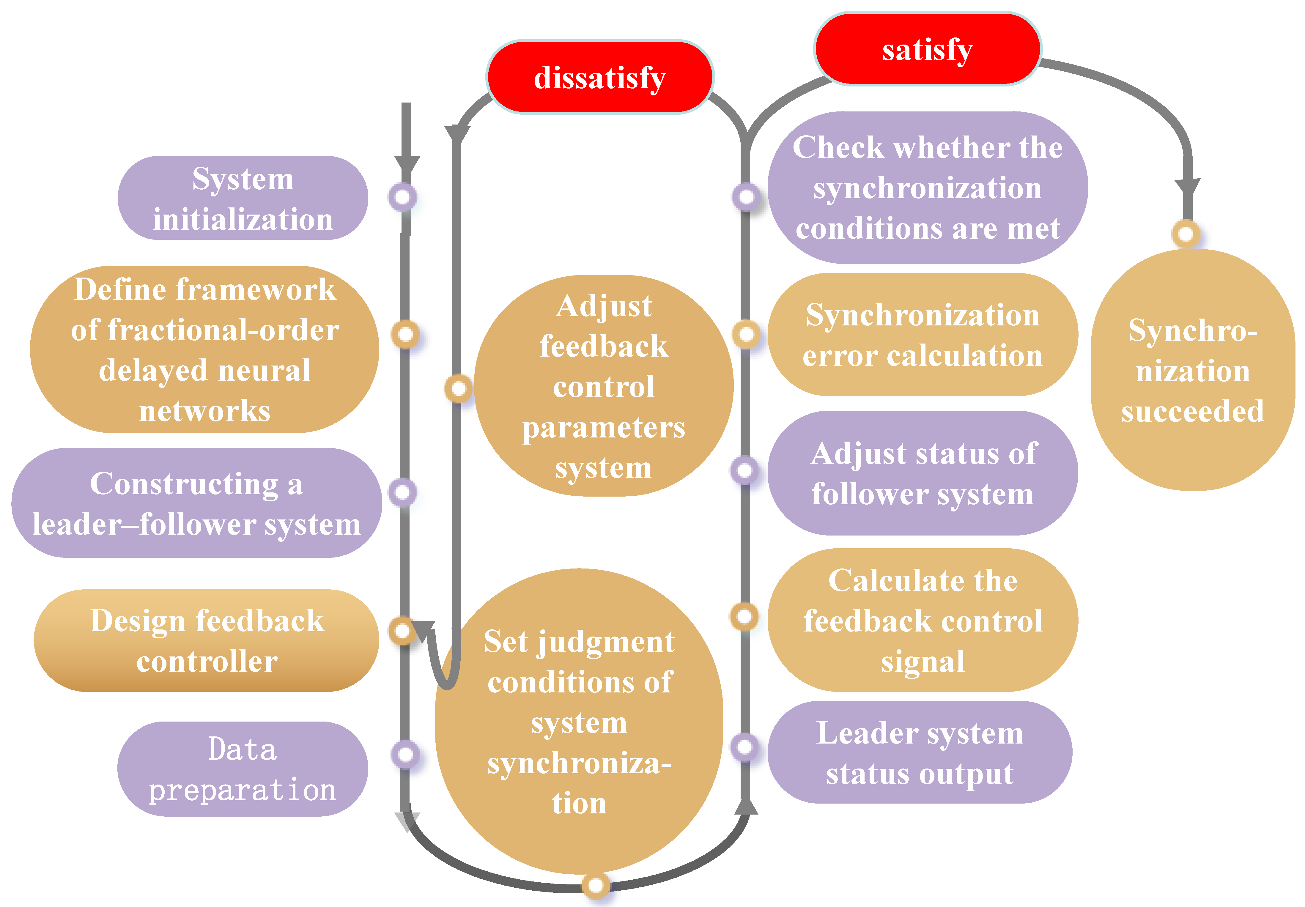
The process framework for synchronizing non-autonomous fractional-order neural networks studied in this article is described as follows (Figure 1):

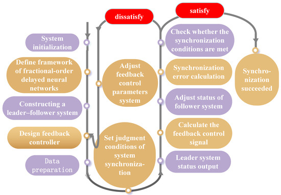
Figure 1. The flowchart of the model and algorithm in this article.

Theorem 1.

Under Assumption 1, and employing Control Scheme 1, we can deduce that the fractional-order, non-autonomous delayed neural network systems (15) and (17) achieve global synchronization.

Proof. 

Based on the error system (20), we devise an appropriate Lyapunov function, denoted as follows:

$$V(t)={\displaystyle \frac{1}{2}}e{(t)}^{T}e(t).$$

(24)

Based on Assumption 1, it follows that $\left|f_j(y_i(t))-f_j(x_i(t))\right|\le l_j\left|e_i(t)\right|, \left|g_j(y_i(t))-g_j(x_i(t))\right|\le h_j\left|e_i(t)\right|.$

Since each element in $A(t)$ and $B(t)$ must be a bounded function in both the leader system (15) and the follower system (17), there exists an upper bound for each element of $A(t)$ and $B(t)$ over the interval $[t_0,\infty )$.

According to Lemmas 1 and 2, we compute the fractional derivative of $V(t)$ and substitute the error system (20) into it. Consequently,

$$\begin{array}{ll}\hfill D^{\alpha }V(t)& =D^{\alpha }\left[{\displaystyle \frac{1}{2}}e{(t)}^{T}e(t)\right]\hfill \\ & \le e{(t)}^T{D}^{\alpha }e(t)\hfill \\ & ={\displaystyle \sum _{i=1}^n{e}_i{(t)}^T}\{-c_i(t)e_i(t)+{\displaystyle \sum _{j=1}^n{a}_{ij}(t)[f_j(y_j(t))-f_j(x_j(t))]}\hfill \\ & +{\displaystyle \sum _{j=1}^n{b}_{ij}(t)[g_j(y_j(t-\tau ))-g_j(x_j(t-\tau ))]}+u_i(t)\}\hfill \\ & \le {\displaystyle \sum _{i=1}^n\left|e_i(t)\right|}\{-c_i(t)e_i(t)+{\displaystyle \sum _{j=1}^n\underset{t_0\le t<+\infty }{\sup }\{a_{ij}(t)\}{l}_j\left|e_i(t)\right|}\hfill \\ & +{\displaystyle \sum _{j=1}^n\underset{t_0\le t<+\infty }{\sup }\{b_{ij}(t)\}{h}_j\left|e_i(t-\tau )\right|}\}-{\displaystyle \sum _{i=1}^n{R}_i{e}_i^2(t)}\hfill \\ & \le {\displaystyle \sum _{i=1}^n-}(c_i(t)+R_i-{\displaystyle \sum _{j=1}^n{l}_j\underset{t_0\le t<+\infty }{\sup }\{a_{ij}(t)\}})e_i^2(t)\hfill \\ & +{\displaystyle \sum _{i=1}^n{\displaystyle \sum _{j=1}^n{h}_j\underset{t_0\le t<+\infty }{\sup }\{b_{ij}(t)\}\left|e_i(t)\right|\left|e_i(t-\tau )\right|}}.\hfill \end{array}$$

(25)

According to the triangle inequality, the following can be concluded:

$$\left|e_i(t)\right|\left|e_i(t-\tau )\right|\le {\displaystyle \frac{1}{2}}{\left|e_i(t)\right|}^2+{\displaystyle \frac{1}{2}}{\left|e_i(t-\tau )\right|}^2.$$

(26)

Substituting (26) into (25) yields the following:

$$\begin{array}{ll}\hfill D^{\alpha }V(t)& \le {\displaystyle \sum _{i=1}^n-}(c_i(t)+R_i-{\displaystyle \sum _{j=1}^n{l}_j\underset{t_0\le t<+\infty }{\sup }\{a_{ij}(t)\}})e_i^2(t)+{\displaystyle \sum _{i=1}^n{\displaystyle \sum _{j=1}^n{h}_j\underset{t_0\le t<+\infty }{\sup }\{b_{ij}(t)\}\left|e_i(t)\right|\left|e_i(t-\tau )\right|}}\hfill \\ & \le -{\displaystyle \frac{1}{2}}{\displaystyle \sum _{i=1}^n(2c_i(t)+2R_i-2{\displaystyle \sum _{j=1}^n{l}_j\underset{t_0\le t<+\infty }{\sup }\{a_{ij}(t)\}}-{\displaystyle \sum _{j=1}^n{h}_j\underset{t_0\le t<+\infty }{\sup }\{b_{ij}(t)\}})e_i^2(t)}\hfill \\ & +{\displaystyle \frac{1}{2}}{\displaystyle \sum _{i=1}^n{\displaystyle \sum _{j=1}^n{h}_j\underset{t_0\le t<+\infty }{\sup }\{b_{ij}(t)\}{e}_i^2(t-\tau )}}\hfill \\ & \le -qV(t)+pV(t-\tau ).\hfill \end{array}$$

(27)

From (27), we obtain the following:

$$D^{\alpha }V(t,x(t)) \le -qV(t,x(t))+p\underset{-\tau \le \theta \le 0}{\sup }V(t+\theta ,x(t+\theta )).$$

(28)

Based on Lemma 3, the fractional-order neural network with the time-delay leader system (15) and the follower system (17) achieve global synchronization under state feedback control (23). □

4. Numerical Simulation

In this section, we present an example of numerical simulation for a fractional-order neural network model incorporating time delays. The instantiated system’s numerical simulation is conducted using Matlab R2024b software, and the resulting simulations are analyzed to validate the accuracy of the aforementioned theoretical analysis and derivations.

Example 1.

Consider the following delayed Caputo fractional-order neural networks as the leader system:

$$\left\{\begin{array}{cc}\hfill D^{0.87}{x}_1(t)=& -(\cos (t)+2)x_1(t)+\cos (t)\tanh (x_1(t))-\cos (t)\tanh (x_2(t))\hfill \\ & -\sin (t)\tanh (x_1(t-0.01))-\cos (t)\tanh (x_2(t-0.01)),\hfill \\ \hfill D^{0.87}{x}_2(t)=& -(\cos (t)+2)x_2(t)+\sin (t)\tanh (x_1(t))+2\cos (t)\tanh (x_2(t))\hfill \\ & -2\sin \left(\mathrm{t}\right)\tanh (x_1(t-0.01))-\sin (t)\tanh (x_2(t-0.01)),\hfill \end{array}\right.$$

(29)

The follower system is described as follows:

$$\left\{\begin{array}{cc}\hfill D^{0.87}{y}_1(t)=& -(\cos (t)+2)y_1(t)+\cos (t)\tanh (y_1(t))-\cos (t)\tanh (y_2(t))\hfill \\ & -\sin (t)\tanh (y_1(t-0.01))-\cos (t)\tanh (y_2(t-0.01))-7(y_1(t)-x_1(t)),\hfill \\ \hfill D^{0.87}{y}_2(t)=& -(\cos (t)+2)y_2(t)+\sin (t)\tanh (y_1(t))+2\cos (t)\tanh (y_2(t))\hfill \\ & \hfill -2\sin \left(\mathrm{t}\right)\tanh (y_1(t-0.01))-\sin (t)\tanh (y_2(t-0.01))-7(y_2(t)-x_2(t)).\end{array}\right.$$

(30)

Comparing systems (29) and (30) with systems (15) and (17), respectively, we can conclude that the correlation weight matrices $A(t)$ and $B(t)$ between neurons at time $t$ and $t-\tau$, the self-correlation weight matrix $C(t)$ of neurons, as well as the excitation functions $f(x(t))$ and $g(x(t))$ of a neuron at time $t$ and $t-\tau$ are as follows, respectively:

$$\begin{gathered} A(t)=\left[\begin{array}{cc}\cos (t)& -\cos (t)\\ \sin (t)& 2\cos (t)\end{array}\right],B(t)=\left[\begin{array}{cc}-\sin (t)& -\cos (t)\\ -2\sin (t)& -\sin (t)\end{array}\right] \\ C(t)=\left[\begin{array}{cc}\cos ( t)+2& 0\\ 0& \cos ( t)+2\end{array}\right],g(x(t))=f(x(t))={(\tanh (x_1(t)),\tanh (x_2(t)))}^T. \end{gathered}$$

And the selection of state variables, time delays, fractional derivatives, and external inputs is as follows:

$$x(t)={(x_1(t),x_2(t))}^T,\tau =0.01,\alpha =0.87 , I={(I_1,I_2)}^T={(0,0)}^T.$$

Through a straightforward calculation, by setting $R_1=R_2=7, l_1=l_2=h_1=h_2=1$, it becomes evident that the systems (29) and (30) fulfill the criteria outlined in Theorem 1. The initial conditions (IC) of the leader system (29) and the follower system (30) are taken as follows:

$$x_1(t_0)=1,x_2(t_0)=3,y_1(t_0)=2,y_2(t_0)=1.$$

(31)

Using MATLAB, we can obtain some numerical solutions of Systems (29) and (30) with the initial conditions (31), which are shown in Figure 2 and Figure 3.

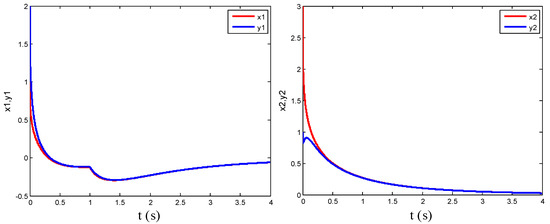
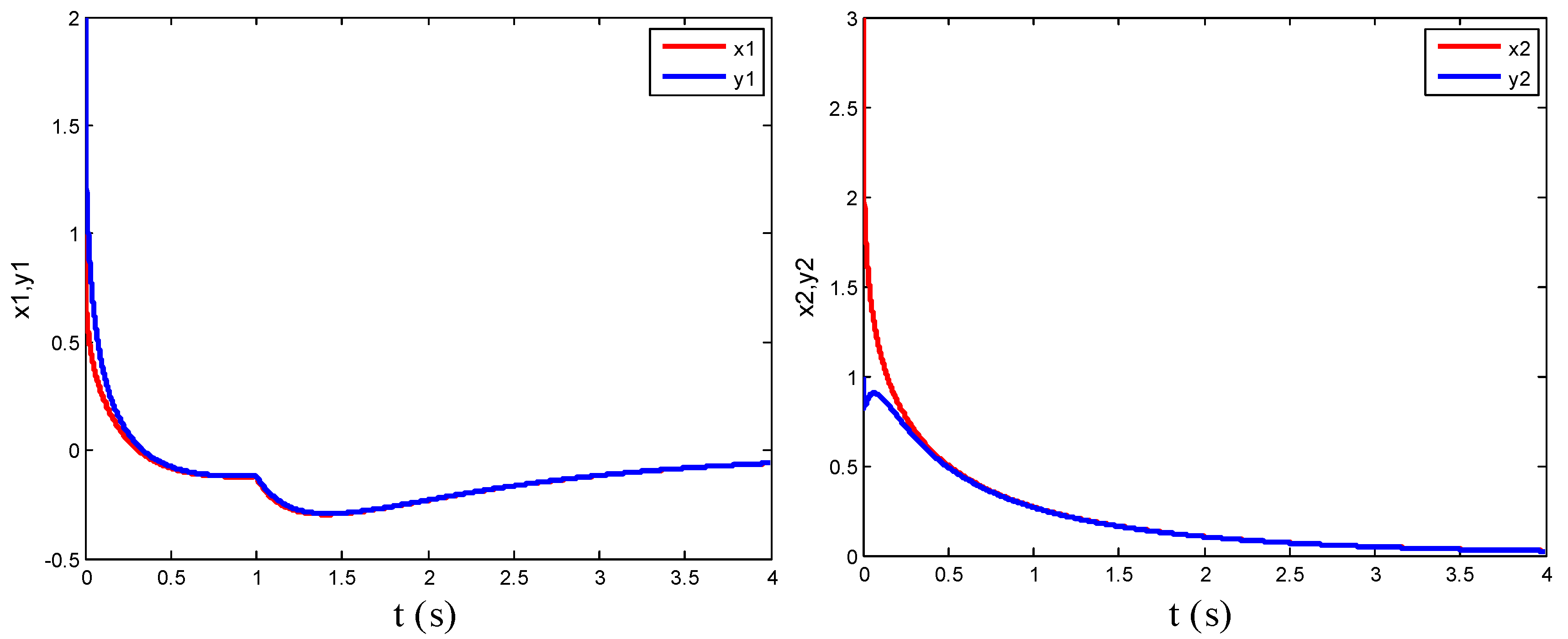
Figure 2. Numerical solution of leader–follower systems (29) and (30) with IC (31).

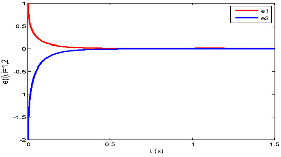
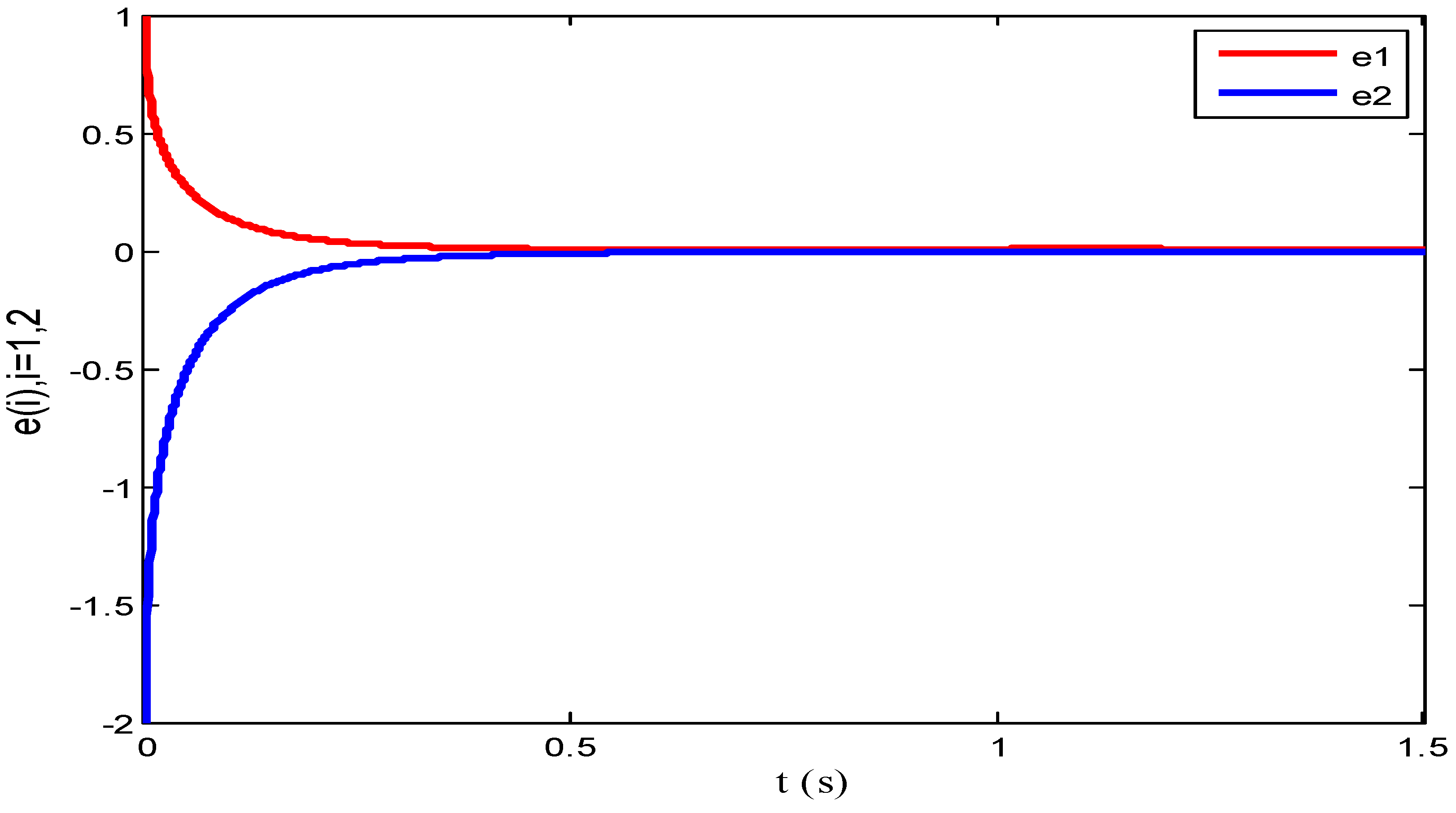
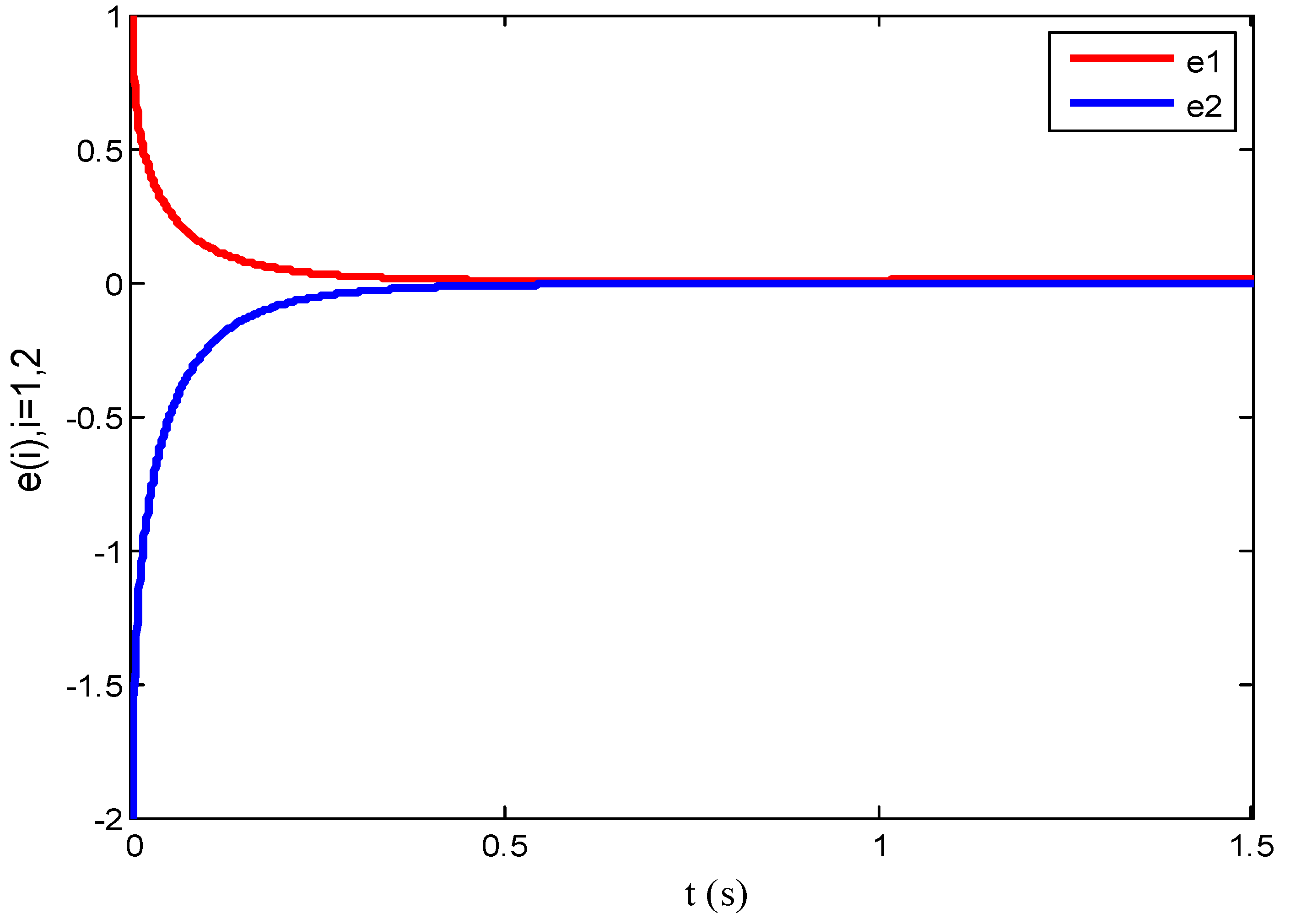
Figure 3. Synchronization errors of leader–follower systems (29) and (30) with IC (31).

As can be observed from Figure 2 and Figure 3, the numerical solution $(x_1,x_2)$ of the leader system (29) and the numerical solution $(y_1,y_2)$ of the corresponding follower system (30) gradually converge and tend towards consistency. The synchronization errors of the leader–follower systems (29) and (30) progressively stabilize at zero. Consequently, it is confirmed that the leader system (29) achieves global synchronization with the follower system (30).

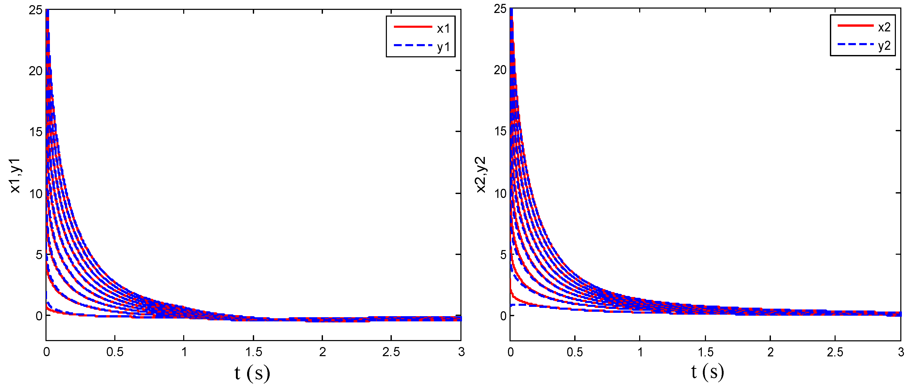
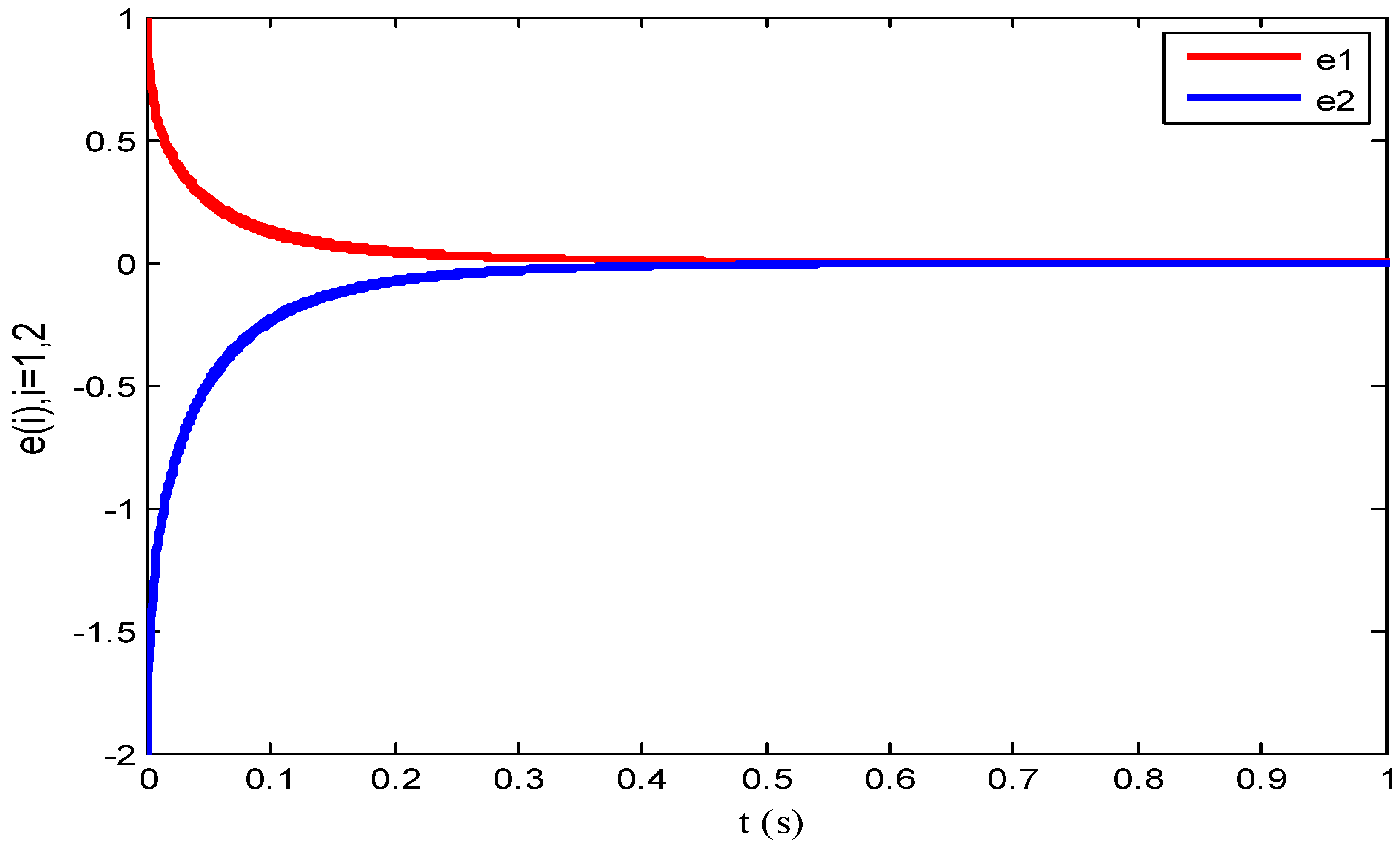
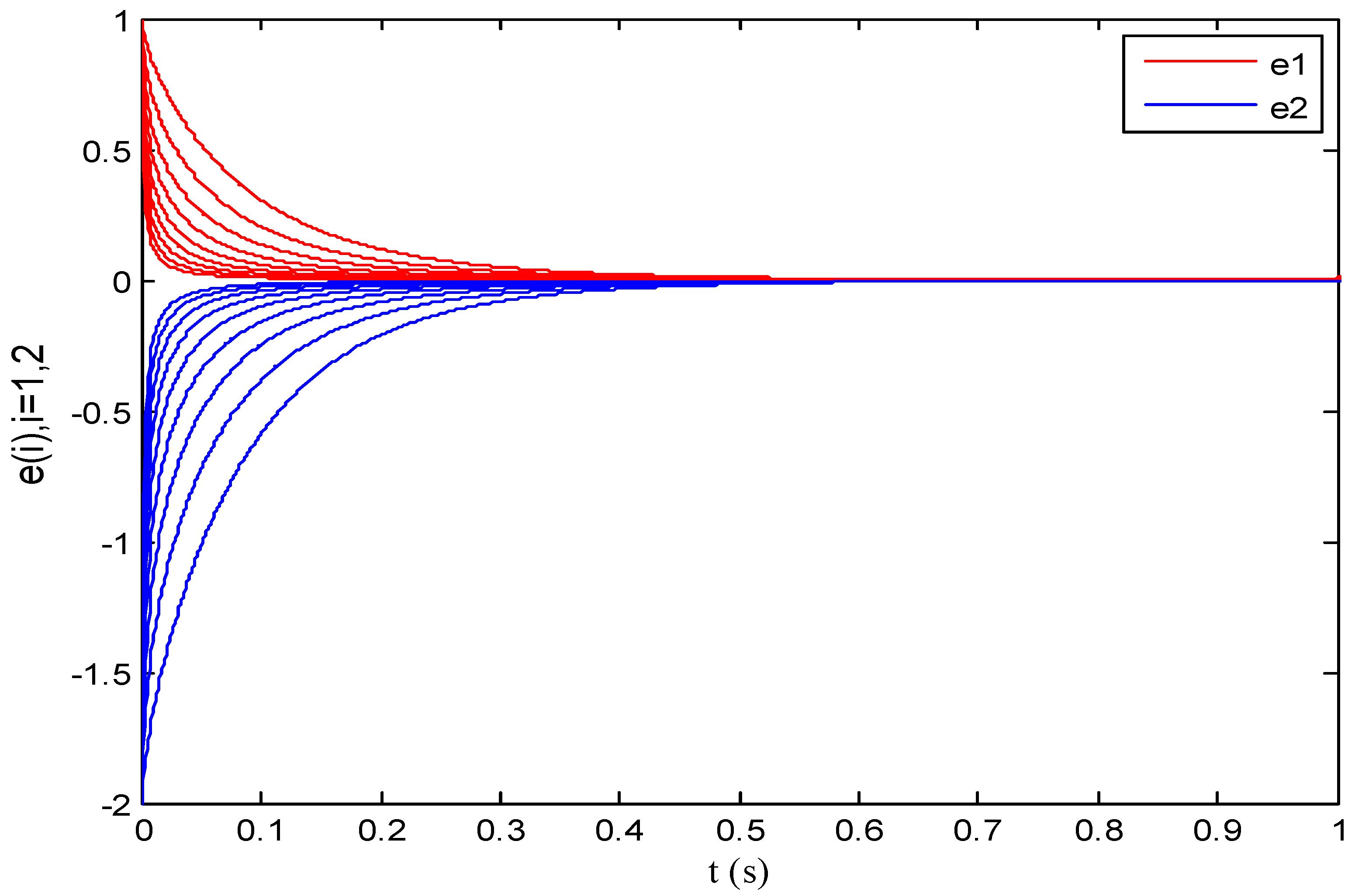
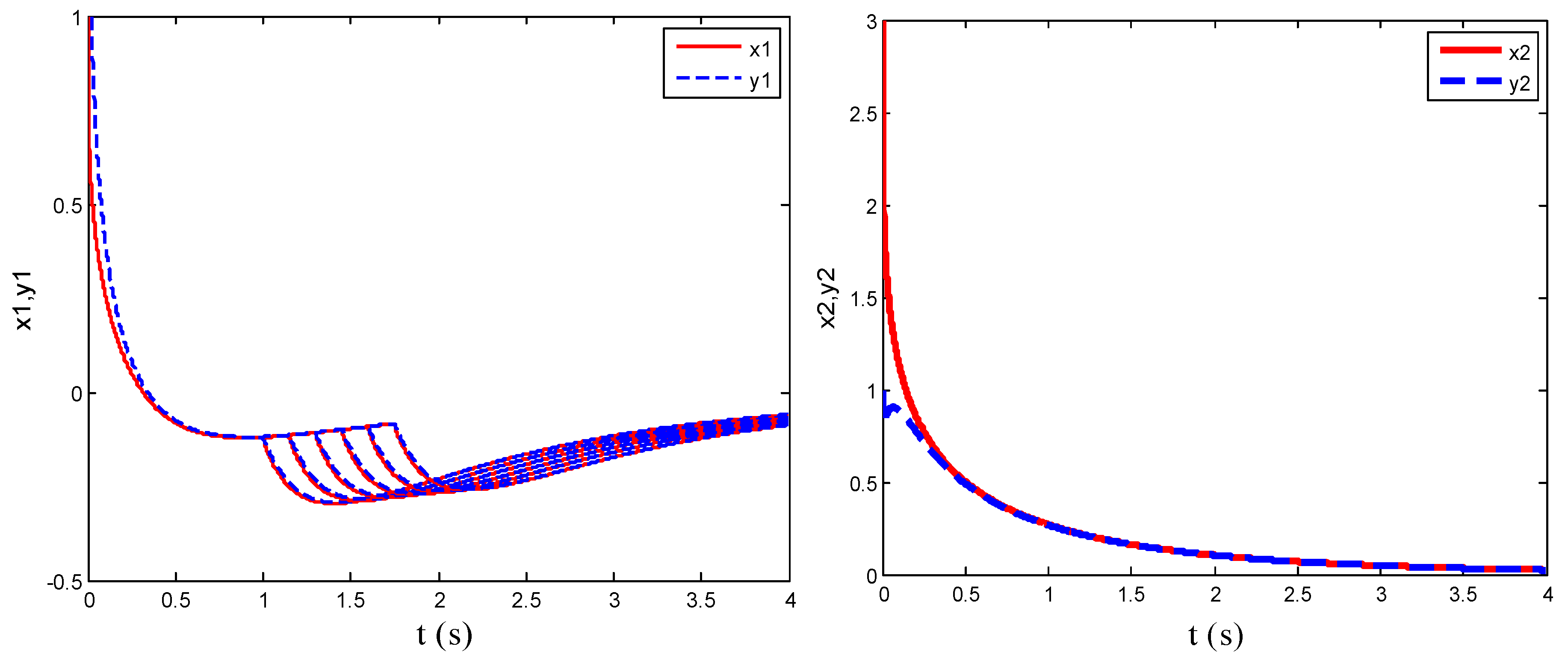
To further validate the global synchronization between the leader system (29) and the follower system (30), we conducted numerical simulations with varying initial conditions, fractional orders, and time delays. The results of these simulations are presented in Figure 4, Figure 5, Figure 6, Figure 7, Figure 8 and Figure 9. Upon observing Figure 4 and Figure 5, it becomes evident that, regardless of the initial conditions chosen, the trajectories of the leader–follower system tend to converge, with the error curve approaching zero. This confirms that the leader system (29) achieves global synchronization with the follower system (30). Similarly, Figure 6 and Figure 7 demonstrate that, as the fractional orders vary, the trajectories of the leader–follower system remain consistent, and the error curve trends towards zero. This further verifies the global synchronization between the leader system (29) and the follower system (30). Furthermore, as shown in Figure 8 and Figure 9, even under different time delays, the trajectories of the leader–follower system continue to align, and the error curve diminishes towards zero. This indicates that the leader system (29) maintains global synchronization with the follower system (30). In summary, regardless of the initial conditions, fractional orders, or time delays selected, the error curve ultimately tends to zero. This conclusively verifies that the leader system (29) is globally synchronized with the follower system (30), and these variations do not impact the synchronization of the system.

Figure 4. Numerical solution of leader–follower systems (29) and (30) under varying IC.

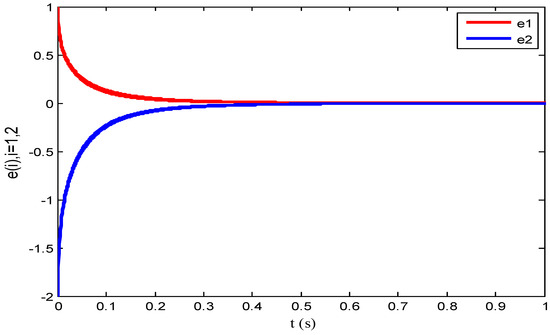
Figure 5. Synchronization errors of leader–follower systems (29) and (30) under varying IC.

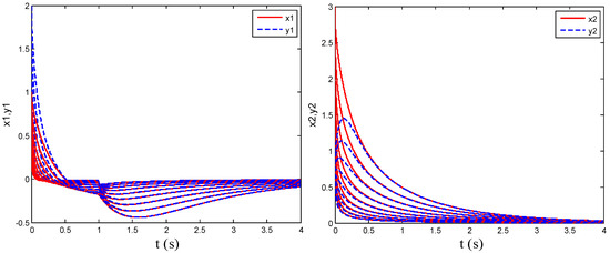
Figure 6. Numerical solution of leader–follower systems (29) and (30) under varying fractional orders.

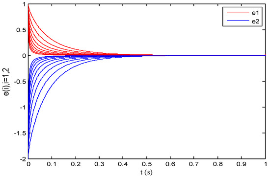
Figure 7. Synchronization errors of leader–follower systems (29) and (30) under varying fractional orders.

Figure 8. Numerical solution of leader–follower systems (29) and (30) under varying delays.

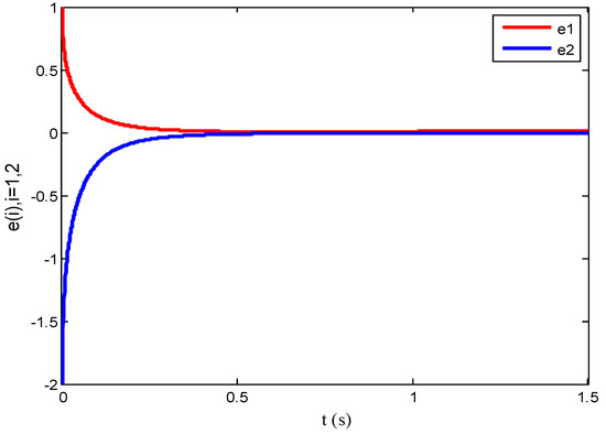
Figure 9. Synchronization errors of leader–follower systems (29) and (30) under varying delays.

5. Summary and Future Work

In this paper, we have delved into the synchronization dynamics of a specific class of fractional-order, delayed, and non-autonomous neural networks. Our primary contribution lies in proposing a streamlined framework for achieving global synchronization within this complex system. By employing a novel state feedback control strategy, we have derived an analytical formula for the synchronization controller. This formula serves as a cornerstone for ensuring the synchronization of the neural networks under consideration. Furthermore, we have leveraged the construction of a Lyapunov function to establish the asymptotic stability of the error system. This stability analysis is crucial for understanding the long-term behavior of the synchronization process. Through rigorous mathematical derivations, we have obtained sufficient conditions that guarantee global synchronization in fractional-order neural networks with time delays and Caputo derivatives. These conditions provide a clear pathway for designing neural networks that exhibit the desired synchronization properties. To validate our theoretical findings, we have conducted numerical simulations. These simulations have demonstrated the effectiveness of our proposed approach in achieving global synchronization. The results obtained from these simulations further reinforce the robustness and practical applicability of our synchronization framework. In addition, the method of constructing Lyapunov functions in references [20,21] is also worthy of our reference and learning in future research work.

Looking ahead, there are several avenues for future research. One potential direction is to extend our synchronization framework to more complex neural network architectures, such as those with spatial dependencies or multiple layers. Additionally, it would be interesting to explore the synchronization properties of neural networks with different types of fractional derivatives, such as the Riemann–Liouville derivative. Furthermore, the impact of various types of delays, such as distributed delays or time-varying delays, on the synchronization of fractional-order neural networks warrants further investigation. Finally, the application of our synchronization framework to real-world problems, such as secure communication or pattern recognition, could provide valuable insights and practical benefits.

References

- Song, Q. Synchronization analysis of coupled connected neural networks with mixed time delays. Neurocomputing 2009, 72, 3907–3914. [Google Scholar] [CrossRef]
- Bao, H.; Park, J.H.; Cao, J. Adaptive synchronization of fractional-order memristor-based neural networks with time delay. Nonlinear Dyn. 2015, 82, 1343–1354. [Google Scholar] [CrossRef]
- Velmurugan, G.; Rakkiyappan, R.; Cao, J. Finite-time synchronization of fractional-order memristor-based neural networks with time delays. Neural Netw. 2016, 73, 36–46. [Google Scholar] [CrossRef] [PubMed]
- Gu, Y.; Yu, Y.; Wang, H. Synchronization for fractional-order time-delayed memristor-based neural networks with parameter uncertainty. J. Frankl. Inst. 2016, 353, 3657–3684. [Google Scholar] [CrossRef]
- Stamova, I.; Stamov, G. Mittag-Leffler synchronization of fractional neural networks with time-varying delays and reaction–diffusion terms using impulsive and linear controllers. Neural Netw. 2017, 96, 22–32. [Google Scholar] [CrossRef] [PubMed]
- Hu, H.-P.; Wang, J.-K.; Xie, F.-L. Dynamics analysis of a new fractional-order hopfield neural network with delay and its generalized projective synchronization. Entropy 2019, 21, 1. [Google Scholar] [CrossRef] [PubMed]
- Zhang, W.; Cao, J.; Wu, R.; Alsaedi, A.; Alsaadi, F.E. Projective synchronization of fractional-order delayed neural networks based on the comparison principle. Adv. Differ. Equ. 2018, 2018, 73. [Google Scholar] [CrossRef]
- Yu, J.; Hu, C.; Jiang, H.; Fan, X. Projective synchronization for fractional neural networks. Neural Netw. 2014, 49, 87–95. [Google Scholar] [CrossRef] [PubMed]
- Hu, T.; Zhang, X.; Zhong, S. Global asymptotic synchronization of nonidentical fractional-order neural networks. Neurocomputing 2018, 313, 39–46. [Google Scholar] [CrossRef]
- Wang, H.; Yu, Y.; Wen, G.; Zhang, S. Stability analysis of fractional-order neural networks with time delay. Neural Process. Lett. 2015, 42, 479–500. [Google Scholar] [CrossRef]
- Peng, X.; Wu, H.; Song, K.; Shi, J. Global synchronization in finite time for fractional-order neural networks with discontinuous activations and time delays. Neural Netw. 2017, 94, 46–54. [Google Scholar] [CrossRef] [PubMed]
- Zhang, L.; Yang, Y.; Wang, F. Synchronization analysis of fractional-order neural networks with time-varying delays via discontinuous neuron activations. Neurocomputing 2018, 275, 40–49. [Google Scholar] [CrossRef]
- Yang, X.; Li, C.; Huang, T.; Song, Q.; Huang, J. Synchronization of fractional-order memristor-based complex-valued neural networks with uncertain parameters and time delays. Chaos Solitons Fractals 2018, 110, 105–123. [Google Scholar] [CrossRef]
- Wang, C.; Yang, Q.; Zhuo, Y.; Li, R. Synchronization analysis of a fractional-order non-autonomous neural network with time delay. Phys. A Stat. Mech. Its Appl. 2020, 549, 124176. [Google Scholar] [CrossRef]
- Wang, C.; Lei, Z.; Jia, L.; Du, Y.; Zhang, Q.; Liu, J. Projective synchronization of a nonautonomous delayed neural networks with Caputo derivative. Int. J. Biomath. 2024, 17, 2350069. [Google Scholar] [CrossRef]
- Pldlubny, I. Fractional Differential Equations; Academic Press: San Diego, CA, USA, 1999. [Google Scholar]
- Anatoly, A.K.; Hari, M.S.; Juan, J.T. Theory and Applications of Fractional Differential Equations; Elsevier Science Ltd.: New York, NY, USA, 2006. [Google Scholar]
- Duarte-Mermoud, M.A.; Aguila-Camacho, N.; Gallegos, J.A.; Castro-Linares, R. Using general quadratic Lyapunov functions to prove Lyapunov uniform stability for fractional order systems. Commun. Nonlinear Sci. Numer. Simul. 2015, 22, 650–659. [Google Scholar] [CrossRef]
- Chen, B.; Chen, J. Razumikhin-type stability theorems for functional fractional-order differential systems and applications. Appl. Math. Comput. 2015, 254, 63–69. [Google Scholar] [CrossRef]
- Dass, A.; Srivastava, S.; Kumar, R. A novel Lyapunov-stability-based recurrent-fuzzy system for the Identification and adaptive control of nonlinear systems. Appl. Soft Comput. 2023, 137, 110161. [Google Scholar] [CrossRef]
- Man, Z.; Wu, H.R.; Liu, S.; Yu, X. A new adaptive backpropagation algorithm based on lyapunov stability theory for neural networks. IEEE Trans. Neural Netw. 2006, 17, 1580–1591. [Google Scholar] [CrossRef] [PubMed]
Disclaimer/Publisher’s Note: The statements, opinions and data contained in all publications are solely those of the individual author(s) and contributor(s) and not of MDPI and/or the editor(s). MDPI and/or the editor(s) disclaim responsibility for any injury to people or property resulting from any ideas, methods, instructions or products referred to in the content. |
© 2025 by the authors. Licensee MDPI, Basel, Switzerland. This article is an open access article distributed under the terms and conditions of the Creative Commons Attribution (CC BY) license (https://creativecommons.org/licenses/by/4.0/).