Abstract
Adversarial transfer learning is extensively applied in computer vision owing to its remarkable capability in addressing domain adaptation. However, its applications in credit scoring remain underexplored due to the complexity of financial data. The performance of traditional credit scoring models relies on the consistency of domain distribution. Any shift in feature distribution leads to a degradation in model accuracy. To address this issue, we propose a domain adaptation framework comprising a transfer learner and a decision tree. The framework integrates the following: (1) feature partitioning through Wassertein relevance metric; (2) adversarial training of the transfer learner using features with significant distributional differences to achieve an inseparable representation of the source and target domains, while the remaining features are utilized for decision tree model training; and (3) a weighted voting method combines the predictions of the transfer learner and the decision tree. The Shapley Additive Explanations (SHAP) method was used to analyze the predictions of the model, providing the importance of individual features and insights into the model’s decision-making process. Experimental results show that our approach improves prediction accuracy by 3.5% compared to existing methods.
Keywords:
credit scoring; domain adaptation; adversarial machine learning; fusion model; explainable artificial intelligence MSC:
68T20
1. Introduction
The 2008 subprime mortgage crisis and the risk control requirements outlined in the revised Basel III agreement underscore the crucial importance of credit risk management in maintaining the stability of the financial system [1]. Credit risk management focuses on accurately evaluating the likelihood that a debtor receiving credit support will fully repay both the principal and interest within the agreed-upon timeframe [2].
Early credit assessments were conducted through credit committee reviews or decisions made by domain experts, the accuracy of which depended on the professional experience of the reviewers, often resulting in inefficiency and bias [3]. With the advancement of machine learning, a range of credit risk scoring models utilizing novel techniques have been developed and optimized, including SVM, decision trees, and naive Bayes (see the review in [4]). These models predict the likelihood of loan default based on various factors, such as borrowers’ past debt performance, income, and assets, thereby enhancing banks’ risk premiums and profitability. However, traditional machine learning methods often require manual feature engineering and data preprocessing, which makes the process of constructing credit scoring models complex and inefficient, thus reducing the adaptability and robustness of credit risk management systems [5].
In recent years, the increasing availability of large digital resources in the financial sector has propelled deep learning-based credit scoring models into the spotlight [6]. By combining simple nonlinear modules to generate multilayer representations, deep learning can uncover latent features in data, extract deeper insights, and improve the accuracy of loan decisions while reducing credit scoring costs. Therefore, designing efficient, accurate, and explainable credit risk scoring models based on deep learning methods has become an important research direction.
Credit risk scoring can be viewed as a binary classification problem. To train a classification model, key features must be extracted from the lender’s information, and, after a performance period, labels of their repayment behavior must be obtained [7]. For newly launched credit products, this introduces two challenges: (1) the applicant’s repayment behavior cannot be observed until the performance period ends, resulting in only unlabeled data initially available, and (2) at the outset of the product launch, only a limited amount of training data are accessible. Consequently, the cost of obtaining a large amount of labeled data for credit scoring in newly launched products hinders the application of deep learning methods [8]. Currently, most credit scoring methods directly fuse samples from old credit scoring tasks with newly acquired samples to train new credit scoring models or fine-tune the parameters of existing models [9]. These methods assume that the features and distributions of both datasets remain consistent to ensure effective generalization of the model. However, due to differences in the characteristics of credit products, such as loan amounts, interest rates, and the types of customers they attract, the data characteristics and distributions often differ. This makes it difficult to achieve a high level of accuracy in traditional credit scoring models which have been trained by fine-tuning only. We need to find a way to address the construction of credit scoring models in scenarios where there are differences in data distribution.
Domain adaptation is a novel approach to training discriminative classifiers or other predictors in the presence of differences between data distributions [10]. By establishing a mapping between the source and target domain distributions, this approach allows the combination of classifiers trained on source domain data with learned mappings, enabling the model to be applied to both source and target domain prediction tasks. Domain adaptation relies on classifiers trained on the source domain and is particularly useful when the target domain is either unlabeled or has few labels. This makes it well suited for modeling credit scoring tasks for newly launched credit products.
In this study, we propose a fusion domain adaptation credit scoring model (FDAT), which consists of a feature divider module, a domain adversarial transfer module, a decision tree model, and a voting fusion module, to address the degradation of model accuracy caused by domain distribution shifts in credit scoring tasks. The main contributions of this work are as follows:
First, we introduce a domain-adaptive transfer learning method for processing structured data, designed for cases where credit data do not follow the same distribution between the source and target domains. The algorithm uses an improved domain adversarial neural network to learn domain-inseparable representations of data samples. Compared to existing domain adaption techniques, the advantages of this improved method are as follows: (1) Combining domain adaptation with deep feature learning ensures that the classifier’s decision is based on a domain-inseparable representation. (2) The deep feature extraction, domain discrimination, and classification processes are integrated into a deep feedforward network, with backpropagation of two loss functions for parameter optimization. (3) The method can be applied to the case where the target domain is unlabeled or has only a small number of labels.
Second, we propose a feature partitioning algorithm based on distributional similarity. It improves the speed of model training and enhances the prediction accuracy. To align features between the source and target domains, we calculate the feature distribution similarity using Wasserstein distance. Features with large distribution differences are used for training the domain adversarial neural network, while the remaining features are used to train an interpretable decision tree model. Finally, the prediction results are integrated via a weighted voting method. Empirical results demonstrate that this approach effectively improves model accuracy and generalization performance.
Third, we provide an explanation for the model’s predictions to meet financial regulatory requirements. The decision tree model inherently offers strong interpretability, while neural networks generally lack this feature. To enhance explainability, we apply the Shapley Additive Explanations (SHAP) method to analyze the changes in feature importance before and after transfer, thereby providing insights to support credit scoring predictions.
The rest of the paper is structured as follows. Section 2 is a systematic literature review that briefly describes the research related to credit scoring and domain adaptation. Section 3 describes the FDAT modeling framework proposed in this paper. Section 4 details the empirical study, including dataset information, hyperparameter tuning, and performance measures. Numerical results and analysis are given in Section 5. The explainability of FDAT is further discussed in Section 6, and future research directions are discussed and conclusions are drawn in Section 7.
2. Related Work
Relevant prior work includes studies of credit scoring models and algorithms to handle distributional shifts in credit scoring problems.
2.1. Credit Scoring Model
Existing credit scoring models can be classified into two main categories: single-structure models and fusion-structure models. Early studies focused on the simple analysis of individual credit using descriptive and exploratory statistical methods. Over time, however, research has shifted towards the integration of machine learning techniques to enhance model scoring.
The origins of credit scoring can be traced back to 1956, when Bill Fair introduced the FICO method. As an ancient single-structure model, it scores an individual’s credit based on a quantitatively weighted score through feature selection by a credit expert [11]. The FICO methodology laid the foundation for the idea of credit scoring using multidimensional weighted evaluations, which is widely used in traditional bank credit scoring practices. However, the results of the FICO model are influenced by credit experts’ selection of features and lack fairness [12]. To mitigate this issue, many researchers have employed more advanced statistical tools, along with machine learning and deep learning techniques, to minimize the influence of human factors.
In terms of the use of statistical tools, credit scoring models based on methods such as logistic regression, naive Bayes, MDP, etc., have been developed [4,13]. These models are simple in structure, offer good interpretability and robustness, and meet the regulatory needs of the financial sector, but the accuracy needs to be improved. Machine learning models, such as decision trees, support vector machines, and BP neural networks, can uncover nonlinear relationships in data and tend to generalize better than traditional statistical models [14]. However, except for decision trees, these models are less interpretable and computationally efficient than methods like logistic regression. Deep learning, a representation learning method, has achieved significant success with image, speech, and text data, but its structure often requires adjustments before it can effectively analyze tabular data in credit scoring. Also, the multilayered, nonlinear nature of deep models makes their decision-making process difficult to interpret.
Different single-structure models each have their own advantages and disadvantages. Fusion structure models combine multiple types of sub-models to leverage the strengths of each and improve overall model performance [15,16]. Based on how the sub-models are combined, fusion models can be categorized into integration-type models and non-integration-type models.
Integration-type models typically involve constructing multiple independent sub-models, which may be of the same or different types. These sub-models’ prediction results are then combined (e.g., through averaging, voting, etc.) to generate a comprehensive prediction that outperforms a single model [17]. For example, Xiao et al. [7] designed a semi-supervised integration method for credit scoring. They first trained an initial integrated model using labeled samples consisting of multiple sub-models. This model then labels unlabeled data through voting, which is added to the training set along with the predicted labels. The model is updated on the new training set, and a cost-sensitive neural network is constructed to complete the credit scoring process. Liu et al. [16] designed a heterogeneous deep forest model based on random forests. This model integrates multiple tree-based ensemble learners at each level, increasing complexity as the dataset size grows and avoiding isomorphic predictions in ensemble frameworks. Runchi et al. [3] employed an integrated approach to improve the logistic model. By adjusting the equilibrium rate of the sub-datasets used to train the sub-models and applying dynamic weighting, their model enhanced its effectiveness in handling imbalanced credit data.
Non-integration-type models focus on combining different types of models or different feature representations to create a new model with superior overall performance. This typically involves processing the outputs of different models (e.g., through weighting, summing, or splicing) to generate final predictions. Many models of this type have shown strong performance in credit scoring. For instance, Shen et al. [18] combined a three-stage decision module with an unsupervised transfer module to align the selected sample distribution with the accepted sample distribution while also selecting the rejected samples. Roseline et al. [19] proposed an LSTM-RNN model that uses a recurrent neural network to fit the samples and an LSTM to extract complex interrelated features from sequential data. Their experimental results showed that the model outperformed single-structure models. To address the issue of spatial local correlation in form data for credit scoring, Qian et al. [20] used soft reordering to adaptively reorganize the one-dimensional form data. This allowed the data to have spatially correlated information, thus enhancing the CNN’s ability to process the data effectively.
Based on the preceding discussion of credit scoring models, it can be observed that fusion models exhibit higher prediction accuracy and robustness compared to single models in credit scoring applications, although their complex structure impairs interpretability. Additionally, most existing studies have concentrated on enhancing the predictive performance of credit scoring models without addressing the shift in credit data distribution between the source and target domains.
2.2. Algorithm to Handle Distributional Difference in the Credit Scoring Problem
The accuracy of credit scoring models, which are essential tools for banks to evaluate loan applicants’ qualifications and determine the credit amounts to be lent, is highly dependent on the consistency of the data distribution. In contrast to other domains, credit data often encounter issues such as missing rejection samples and imbalanced sample distribution, which significantly exacerbate the distributional discrepancies between the credit data used to train the model (the source domain) and the actual credit data used during model application (the target domain), ultimately reducing the model’s accuracy [21].
The reasons for distributional shifts in credit assessment can be classified into two categories: sample selection bias and changes in application scenarios. As banks and financial institutions lack access to information about unapproved loan applicants, most data used for constructing credit scoring models are derived from approved customers, leading to a sample selection bias in relation to the true distribution [22]. Researchers often consider this sample selection bias as a missing data issue, treating applicants’ insufficient credit history or partial data loss as random missing (MAR) and missing rejection samples as non-random missing (MNAR), with the process of addressing missing data referred to as rejection inference [23].
Under the MAR assumption, Li et al. [24] employed a semi-supervised SVM model for rejection inference to determine the support hyperplane by incorporating both accepted and rejected samples, with results outperforming traditional supervised credit scoring methods. Kang et al. [25] introduced the label spreading method into credit scoring and employed a graph-based semi-supervised learning technique with SMOTE for rejection inference, improving the model’s performance in handling unbalanced data. Concurrently, deep generative methods have also been incorporated into rejection inference. Mancisidor et al. [26] combined Gaussian mixture models and auxiliary variables within a semi-supervised framework with generative models, utilizing efficient stochastic gradient optimization to enhance the model’s capacity to handle large datasets. This approach is advantageous, as model performance improves progressively with increased training data. Shen et al. [21] employed a semi-supervised approach based on joint distributional adaptivity to a supervised form, reducing the distributional discrepancy between acceptance and rejection sample sets and achieving state-of-the-art performance in the semi-supervised rejection inference credit assessment task.
In summary, existing studies have demonstrated an improved ability to address sample selection bias, which results in data distribution shift, through a variety of rejection inference techniques. However, the existing research does not consider the problem of data distribution shift faced by credit scoring models.
With the advent of the big data era, the impact of shifting application scenarios on the accuracy of credit scoring has become increasingly significant. Compared to traditional bank lending practices, diversified online lending products cater to different audiences, which often results in a distributional shift between the training data and actual data. As a result, it is difficult to directly apply a credit scoring model developed for one product to other products.
Domain adaptation is a primary approach to address distribution bias, applicable when the source and target tasks are the same in transfer process but the data distributions in the source and target domains differ. Unlike traditional credit scoring models, domain adaptation models use a small amount of target domain unlabeled data. Figure 1 illustrates the classification of domain adaptation methods. Depending on whether intermediate domains are constructed during transfer, domain adaptation methods can be divided into single-step and multi-step approaches.
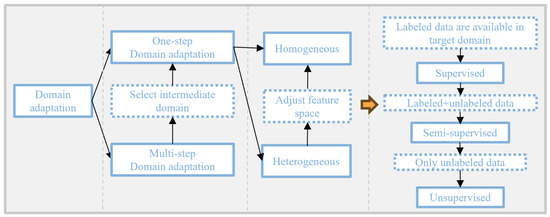
Figure 1.
Classification of existing domain adaptation methods.
In cases where the shift between the source and target domains is substantial (e.g., when the source domain contains text data and the target domain contains image data), the transfer task may need to be broken into multiple mappings for multi-step domain adaptation. For instance, in situations where the distribution shift in an image classification task is large, Xiang et al. [27] designed a multi-step domain-adaptive image classification network with an attention mechanism to complete the domain adaptation task in two steps. The first step uses the attention mechanism to merge the source and target domain data, while the second step aligns the source and target domains at both the pixel and global levels. This method effectively mitigates model performance degradation caused by significant distributional differences between the source and target domains in image classification tasks.
Furthermore, single-step domain adaptation can be further divided into homogeneous domain adaptation (where the data space is consistent, but distributions differ) and heterogeneous domain adaptation (where both the data space and distributions differ), depending on the source and target domain data [28]. In the case of heterogeneous domain adaptation, features are challenging to automatically align in the neural networks used for transfer. Thus, a feature converter must be introduced before mapping the source and target domain features. The feature converter is based on the distributional information between the source and target domains to achieve generalized feature alignment. Building on this concept, Gupta et al. [29] designed the Cross Modal Distillation method, which first learns the structure of the feature converter from a large labeled modality (the source domain) and then uses it to extract features from an unlabeled modality (the target domain), facilitating transfer supervision between images from different modalities.
For credit scoring tasks, which typically rely on tabular data with similar features, only a single-step domain adaptation is necessary. Since different credit datasets usually have different data spaces, a feature converter needs to be designed to resolve the heterogeneity between the data domains. For example, AghaeiRad et al. [30] designed an unsupervised transfer model based on the self-organising map (SOM), which clusters the knowledge discovered by the SOM and passes it into the FNN to achieve more accurate credit scoring.
The core of domain adaptation modeling lies in measuring and adjusting the distributional differences between the source and target domains. Early research focused on the linear assumption that the distributional bias could be represented by a linear mapping [31]. Over time, nonlinear representations (e.g., neural network-based models) were introduced to improve the handling of distributional differences, particularly through the development of robust representation principles in the denoising autoencoder paradigm [32]. More recently, many unsupervised methods have been applied to address distributional bias. Zhang et al. [33] reweighted the sample data to adjust the distributions, but this approach struggled with feature space variations. Zhang et al. developed a method to learn feature transformation matrices online in the original feature space by measuring the similarities between distributions. They then mapped these original features to the kernel space using Online Single Kernel Feature Transformation (OSKFT), thus learning nonlinear feature transformations. Compared to sample reweighting, this method—matching kernels to regenerate the mean of the Hilbert space distribution—can handle feature space variations. However, it suffers from unidirectionality in its mapping without further improvements.
Our approach also aims to match the spatial distributions of features between the source and target domains. However, unlike sample reweighting or direct mapping from the source domain to the target domain, it leverages the concept of domain-adversarial training [34]. Specifically, we use the Wasserstein metric between features and the discriminative properties between domains as criteria to classify feature subsets. We then confrontationally learn a mapping such that, after passing through this mapping, the data from the source and target domains become indistinguishable to the domain discriminator. Figure 2 illustrates the difference between our method and the previous methods.
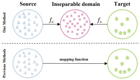
Figure 2.
Differences between our domain adaptation method and other methods. (Top) Past research maps source domains to target domains. (Bottom) Our suggested method builds an inseparable domain that accomplishes domain indiscriminately across credit data.
3. Methodology
In this study, we propose a fusion model framework based on domain adversarial transfer learning (FDAT). The model aims to address the issue of accuracy degradation caused by shifts in feature distribution between training data and actual data in credit scoring tasks. Additionally, it seeks to improve model generalization and maintain a certain degree of interpretability. Figure 3 illustrates the structure of the proposed model, which includes a feature divider module, a domain adversarial transfer module, a decision tree model, and a voting fusion module.
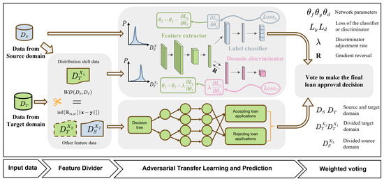
Figure 3.
Framework of the proposed model.
Given a set of source and target domain credit data to be transfered, as shown in Figure 3, in the feature divider module, the Wasserstein distance is used to measure the similarity of feature distributions between the source and target domains. The target domain features are then divided based on similarity ranking into two categories: features with distributional bias and other features. The former is used for training in the domain adversarial transfer module, while the latter is input into the decision tree model. FDAT divides the features and uses them for sub-model training and fuses them at the model output. This approach ensures model training efficiency and full utilization of features.
In the domain adversarial transfer module, the data are transformed by the feature extractor. The output of the feature extractor is then connected to both the label classifier and the domain discriminator. The classifier uses the processed data to predict whether a lender will default on the loan, while the domain discriminator attempts to distinguish whether each data point originates from the source or target domain. It is important to note that, in the domain adversarial transfer module, only the sample labels from the source domain data are used, while the target domain data undergo unsupervised training.
The decision tree model is trained and used for prediction with features that exhibit smaller distributional shifts between the source and target domain data. The use of target domain data depends on its labeling. The final fusion of predictions from the domain adversarial transfer module and the decision tree is performed using a weighted voting method.
3.1. Dividing Feature Based on Wassertein Distance
The domain-adversarial transfer module is a crucial component of FDAT, designed to address data distribution shift. However, not all features should be included in the training process. Including features with similar distributions in both the source and target domains in the domain-adversarial transfer module can increase model training time and potentially result in the loss of feature information during the extraction process. Therefore, in the initial phase of the model, we employ a feature divider based on Wasserstein distance to measure the similarity between features in the source and target domains for feature selection.
Previous studies have used the Kullback–Leibler (KL) divergence to measure the similarity between two distributions. However, KL divergence is asymmetric, meaning that for a set of credit feature distributions P, Q to be measured,
In contrast to KL divergence, the Wasserstein distance quantifies the minimum effort required to transform the probability density of one distribution to match the other [22]. Its advantages include that the Wasserstein distance is symmetric and satisfies the triangle inequality, ensuring that for two characteristic distributions, there is a unique Wasserstein distance corresponding to them. Secondly, since the Wasserstein distance represents a lower bound for the shift between distributions, it is more accurate and sensitive to distributional changes. It is particularly effective at measuring the distance between two distributions when there is little or no overlap between the source and target domain distributions, making it robust to complex distributions and noise perturbations. Finally, the Wasserstein distance exhibits better continuity during changes in similarity between two distributions, partially addressing the gradient explosion problem.
Specifically, we pair similar features in the source and target domains, compute the Wassertein distance for each pair of source and target domain features, and normalize within the group by Equation (2),
where W denotes the Wassertein distance vector between source and target domain features, x is the component of the Wassertein distance vector that denotes the W value for each set of paired source and target domain features. is the normalized W vector. According to Panaretos’ suggestion, features with normalized values greater than 0.35 are used for subsequent domain-adversarial transfer training, and the rest of the features are processed by the decision tree model. Theorem 1 below gives the definition of Wassertein distance in the context of this study.
Theorem 1.
Assume there exists a set of source domain distributions and target domain distributions , both defined over a common feature space X. The set of joint probability distributions consists of the marginal distributions from the source domain and from the target domain is . Define as the probability of appearing in the marginal distributions of the source domain and appearing in the marginal distributions of the target domain at the same time. The lower bound of the expectation of the distances between and is defined as:
which represents the Wasserstein distance between the feature space of the source and target domains in the context of the credit scoring task.
After the feature divider, the target domain feature space is divided into ,, corresponding to the feature distributions and , where there is a large difference between and the corresponding feature distribution in the source domain.
3.2. Credit Data Domain Adaption Based on Domain-Adversarial Transfer Learning
The domain-adversarial transfer module in the model performs transfer learning on features that exhibit substantial distributional shift between the source and target domains, which are selected by the feature divider. In this section, we first define the domain adaption task in the context of credit scoring, then introduce the concept and theory of domain-adversarial transfer learning, and finally, provide details regarding the design of the module for the credit scoring task.
3.2.1. Domain Adaption Task in Credit Scoring
Consider the following scenario: let X represent the feature space of the sample, and be the set of labels, where 1 indicates the approval of a loan application and 0 indicates rejection. For two different types of credit products, different products may gather distinct customer information, leading to variations in the feature space X. Additionally, even when the feature space is consistent, the distribution may still differ. Suppose the data distribution of labeled credit products used to train the old model is denoted as , while the data distribution of unlabeled credit products, which serve as the transfer target, is denoted as (the model applies to the labelled case as well). The risk of misclassification for the classifier in the target domain is shown in Equation (4). The domain transfer task aims to learn a classifier in the transfer learner from a series of independently and identically distributed (i.i.d.) labeled samples drawn from and i.i.d. unlabeled samples from , such that the risk of misclassification in the target domain remains low, even when no labeled information is available from the target domain.
3.2.2. Domain-Adversarial Transfer Learning Theory
As discussed in the Introduction, the new credit product lacks labeled data, meaning only unsupervised learning can be applied. In contrast, the source domain for the old product has an ample amount of historical credit data. The transfer learning module should first train the model using the labeled data from the source domain, and then fine-tune it using the unlabeled data from the target domain. Although there is a small shift in the data distributions between the target and source domains, when the variability is minimal, the accuracy of the fine-tuned model on the source domain data can serve as a reasonable approximation of its performance on the target domain data.
The idea originates from Ben-David’s 2006 work, which demonstrated that the generalization bound of a classifier’s misclassification risk for unlabeled target domain data depends on four factors: (1) the misclassification risk in the source domain, (2) the estimated value of the divergency between the source and target domain distributions, (3) the hypothesis class corresponding to the VC-dimension of the reproducing kernel Hilbert space, and (4) the magnitude of the sample sizes in both the source and target domains [35]. The definition of divergency and the formulation of Ben-David’s theory in the context of credit scoring are provided below.
Theorem 2.
For the credit data source domain edge distribution and target domain edge distribution , the divergency between and is, under the hypothesis class , defined as:
Theorem 3.
Define as a hypothesis class with VC dimension d. For datasets and drawn from the credit data source and target domains, respectively, at a confidence level δ, for each , the following condition is satisfied:
where and . denotes that when the expression m is true, takes the value 1; otherwise, it takes the value 0.
The above theorem asserts that to minimize the risk of misclassification in the classifier’s prediction on target domain credit data, the model must be designed to simultaneously fulfill two conditions: (1) achieving a low misclassification risk in the source domain data, and (2) maintaining a low H divergency between the source and target domains. However, the accuracy of the model is dependent on the information provided by the feature distribution. The shift in distribution between the source and target domains inherently enhances the model’s discriminative ability. When the model is trained using source domain data and labels, it will inevitably be influenced by the distributional shifts. Moreover, attempting to eliminate the shift between the source and target domains by training the model with domain-indistinguishable features leads to a loss of distributional information, which, in turn, negatively impacts the model’s accuracy. Consequently, it is necessary to balance model accuracy with the divergency values.
This concept is implemented in our transfer module, which comprises four components: feature extractor, label classifier, gradient reversal structure, and domain discriminator. In the feature extractor, the neural network learns a function f that maps the source and target domain data to a new feature space. The output of the feature extractor is forwarded to the classifier, which aims to predict the source domain labels as accurately as possible, and to the domain discriminator, which attempts to distinguish whether the feature extractor’s output originates from the source or target domain. The gradient reversal structure is employed to negate the gradient propagated back from the domain discriminator, completing the adversarial interaction between the domain discriminator and the label classifier. As a result, the gradient computed from the loss functions of both the classifier and the domain discriminator during backpropagation, in addition to influencing their respective internal parameters, will also impact the feature extractor, guiding it to generate domain-indistinguishable features.
3.2.3. Model Practice Details in Credit Scoring Tasks
Although the three main components of domain adversarial transfer laearning, the feature extractor, the domain discriminator, and the label classifier, can be any sub-model structure capable of backpropagation, due to the low dimensionality of the credit data compared to the computer vision task, the use of deep neural networks tends to cause an overfitting problem, so a network structure with a slightly higher number of layers can be used for the feature extractor, and a small number of hidden layers can be used for the classifiers and the domain discriminators.
For illustration, we assume that the feature extractor, domain discriminator, and label classifier are all composed of single-layer neural networks. As shown in Figure 3, the target domain, after being processed by the feature divider, is partitioned into two parts: and . The data from the target domain and the source domain are ‘confluent’ in the domain adversarial transfer module, denoted as and , respectively. We assume that the source and target domain data both have k dimensions, i.e., , and that the feature extractor maps the data into an m-dimensional feature space via . The parameter matrix of the neural network is denoted as , and to incorporate the nonlinear properties, a sigmoid activation function is applied at the last layer of the feature extractor. Specifically, and are first passed through the domain adversarial transfer module to complete the mapping, as shown in Equation (7).
where .
The next training process can be divided into two steps.
Step 1: The source domain data is forward propagated to the classifier part as input after processing by f. The classifier performs the mapping, denoted as . The output of the mapping lies between 0 and 1, representing the model’s prediction of the probability of default or on-time payment for a customer. Assume the matrix vector pair of the classifier parameters, denoted as , and in the last layer of the neural network, the softmax activation function is applied to each sample. The formula is as follows:
where .
Finally the logarithmic loss function is used as the classifier loss for backpropagation training and the loss function is shown in Equation (9).Thus, the first step is actually completing the optimization as shown in Equation (10).
Step 2: The source domain data and the target domain data processed by the f function are forward propagated to the domain discriminator part as input. Similar to the classifier, the domain discriminator implements the mapping , and the matrix vector pair of the domain discriminator parameters is denoted as . The mapping function is expressed as:
The domain discriminator has the same loss function as the classifier, as shown in Equation (12), only the labels used are different.
The source domain data are passed through the classifier using labels indicating whether the customer has defaulted or not. When the source and target domains pass through the domain discriminator, the labels for the source domain are all 1s, while the labels for the target domain are all 0s. The goal is to make it difficult for the domain classifier to distinguish between the source of each data sample. Therefore, the optimization objective of the second step is defined as follows:
It can be observed that there is a conflict between the optimization objectives of the first and second steps. In the first step, the goal is to adjust the feature extractor to achieve the best classification results. In contrast, the second step aims to disrupt the effect of the feature extractor so that the features it provides cannot be used for predicting the source domain data. In actual prediction, the and e parameters are not used, but only as intermediate variables for backpropagation when updating the parameters and b. Therefore, the optimization objective of the domain discriminator can be seen as a form of regularization for the and b parameters. To facilitate tuning, we add a regularization factor to the loss function of the domain discriminator. Consequently, we can express the overall optimization objective as shown in Equation (14).
At each iteration, two backpropagation steps are used to sequentially complete the first and second parts of the parameter optimization. This process ultimately results in the creation of a high-performance classifier, which successfully trains the adversarial transfer part.
3.3. Fusion Model Through Voting
After the transfer learner and the decision tree have completed their predictions, the final stage of weighted voting prediction is initiated, which is designed to give more importance to certain modules that are more representative of the underlying data distribution. The decision tree, trained using the feature from the feature divider, and the results predicted by the transfer learner are weighted and combined to make the final judgment. When integrating the results of the credit scoring model via the weighted voting method, the optimal weights are influenced by the dataset size. For smaller credit datasets, the transfer learner learns less valid information and is prone to overfitting, so the weight of the decision tree model should be increased. Conversely, for larger datasets, the decision tree model struggles to capture deeper features, and the transfer learner performs better in terms of accuracy, necessitating an increased weight for its predictions.
To determine the optimal weights for voting integration under different data volumes, we use the Chinese dataset for testing. The dataset is divided into three sizes: 10,000, 100,000, and 200,000 data points. The Chinese dataset is randomly sampled into 10 groups for each dataset size, numbered 1 through 10. Following this, we set the weightings for the transfer learner and the decision tree. For the i-th group of data, the weight ratio between the two modules is .
Finally, the optimal weights are selected based on the integration accuracy. The optimal weights for each dataset size are presented in Table 1.

Table 1.
Optimal weight allocation for transfer model prediction and decision tree prediction for different-sized datasets.
The effectiveness of the final decision is influenced by the performance of both the feature divider and the transfer learner. The quality of the feature divider directly impacts the performance of the decision tree. When features with significant distribution shifts are assigned to the decision tree, its generation and pruning are greatly affected. This is because the same feature, when chosen as a node for both the source and target domains, can result in different gains in classification accuracy. A node that provides the maximum gain in the source domain may lose its effectiveness in the target domain. The impact of the transfer learner is even more significant. If the feature extractor fails to capture domain-invariant information, the model’s accuracy in the target domain will inevitably be low. Therefore, each component of the model plays a crucial role in ensuring overall performance.
4. Empirical Study
This section details the dataset used in the experiment, the model’s hyperparameter tuning process, and the evaluation metrics for assessing model performance.
4.1. Credit Dataset
Table 2 presents four public credit datasets, each with varying sizes and imbalance rates, to comprehensively evaluate the model’s capabilities. The “German” dataset [36] is sourced from the UCI international public database, containing credit data from German banks. The “give-credit” [37] and “credit-fraud” [38] datasets are derived from the Give Me Some Credit and Credit Card Fraud Detection data science competitions, respectively, with the former being a widely utilized dataset for credit scoring research and the latter tailored for credit card fraud detection tasks. The “Chinese” dataset [39] consists of one million samples from the AliTianchi Chinese credit dataset. Prior to model construction, the dataset is processed to fill missing values, convert all features to numeric types, and categorize sample labels into two categories: good credit (non-fraudulent) and bad credit (fraudulent), labeled as 1 and 0, respectively. Due to the large size of the “Chinese” dataset, the data are loaded into the training program in 20 separate batches.
Table 2.
Data descriptions.
4.2. Implementation Details
To ensure the validity and comparability of the experimental results, the hyperparameters must be carefully tuned. When a dataset is used as the source domain, it is entirely utilized for model training. However, when used as the target domain, the dataset is randomly divided into two parts: 80% for the training set and 20% for the test set. To construct the validation set, 20% of the samples from the training set are randomly selected. Consequently, the extracted training, test, and validation sets maintain the same distribution as the original data.
Given that the model has numerous hyperparameters, using grid search for exhaustive optimization is not feasible. Instead, we employ random search, which generates a specified number of random hyperparameter combinations within a defined range. The optimal hyperparameter combination is selected based on classification scores from the validation set, which ensures the speed of convergence of the model and the effectiveness of hyperparameter tuning. The hyperparameter search spaces for all experimental models are listed in Table 3. To minimize the impact of sample differences, the same training, validation, and test sets are used consistently across all models for training, hyperparameter tuning, and evaluation.
Table 3.
Hyperparameters optimization list and search space of benchmark models.
All experiments were conducted using the PyTorch platform (version 2.2.1) on a PC equipped with a 12th-gen Intel i7-12700H processor (manufactured by Intel Corporation, Santa Clara, CA, USA)and an NVIDIA RTX 3060 graphics card (manufactured by NVIDIA Corporation, Santa Clara, CA, USA). To ensure the reliability of the results, each experiment was run 10 times, and the results were averaged.
4.3. Evaluation Metrics
In credit scoring problems, the selection of appropriate metrics is crucial for comprehensively assessing model effectiveness and guiding model tuning [40]. Therefore, we selected six widely used evaluation metrics in credit scoring field: accuracy, AUC, sensitivity, specificity, BS, and KS. As a metric that considers prediction accuracy in both categories, Accuracy is an indicator of the proportion of correctly predicted samples in an experiment relative to the total number of samples, as defined in Equation (15). AUC is a widely used metric which is less affected by changes in the distribution of the test set [41]. Sensitivity measures the model’s ability to identify default and minority samples, while the specificity measures model’s ability to recognize non-default and majority samples. They are defined using Equations (16) and (17). BS is used as a mean square error (MSE) in classification problems [42]. In a binary classification problem, it is defined as Equation (18), where represents the predicted probability, is the actual label, and N is the total number of samples. KS is numerically equal to the maximum value of the difference between the false-positive rate (FPR) curve and the true-positive rate (TPR) [43]. The larger the KS value, the better the model’s ability to distinguish between borrowers who make on-time payments and those who default on their loans. It is defined as Equation (19). More information on metrics can be found in reference [44].
5. Empirical Results and Analysis
5.1. Ablation Study Results
In this section, we present an ablation study of the FDAT model. To investigate whether the improvement in credit scoring performance can be attributed to the synergistic effect of narrowing distributional shifts and the fusion judgment mechanism (i.e., the combined effect of the three modules of the model), we design four ablation experiments for comparative validation. First, we omit the feature divider module in order to verify whether the feature divider can bring about an improvement in model accuracy by selecting feature inputs for the sub-module. Since this module affects the input features of both the transfer learner and the decision tree, we design two sets of experiments: FS1, in which feature divider is omitted, meaning that both the adversarial transfer module and the decision tree model have access to all feature data, which is akin to the general model fusion method, and FS2, in which the features are randomly partitioned, ensuring that 75% of the features are input into the transfer learner, while the remaining features are used for decision tree training. Additionally, FNN substitutes a BP neural network for the transfer learner, with the number of layers in the BP neural network equal to the sum of the layers of the feature extractor and classifier networks to maintain experimental validity. This is to simulate traditional neural network models that lack migration learning. Finally, we remove the decision tree model and construct the FDA, which makes predictions based on a single judgment using only the feature divider and transfer learner, meaning that only a subset of the features is used for training.
It is important to note that dataset size and imbalance can influence model performance. The size of the dataset affects the depth of model learning, and the imbalance rate may make it difficult for the model to accurately predict types with fewer samples. To comprehensively explore the usage scenarios of FDAT, we report the accuracy results of the five models across 12 categories of combinations, using four datasets as both the source-domain and target-domain datasets.
As shown in Table 4, FDAT and FS1 demonstrate superior results across the combination of 12 classes. FDAT excels with large-scale datasets, while FS1 outperforms FDAT when the source and target domains are small-scale datasets. This suggests that the feature divider’s control over the input features of both the transfer learner and the decision tree model is more effective on large-scale datasets. In contrast, for small-scale datasets, it is more beneficial to enable the model to fully leverage the source domain features. This is corroborated by the comparison between FS1 and FS2, where FS1 performs better on small-scale datasets, while no significant performance difference is observed between the two on large-scale datasets. Additionally, FDAT outperforms FDA in all experiments, highlighting the effectiveness of the model fusion mechanism, which enhances prediction accuracy through voting judgment. FNN shows the worst performance in most experiments due to the absence of the domain-adversarial transfer module, with the shift between source and target domain distributions significantly impacting prediction accuracy. Furthermore, we observe that the accuracy is also influenced by the imbalance rate of the target domain data. The credit-fraud dataset, with its extremely high imbalance rate, results in model accuracy ranging from 0.6 to 0.7 when used as the target domain, which is notably lower than that of the other datasets.
Table 4.
Results of ablation experiments: accuracy of credit scores for different source and target domains.
In order to obtain convincing conclusions, we performed statistical significance tests based on the Friedman and post hoc Nemenyi tests for the ablation study. The results of the tests are presented in a visualized form. As shown in Figure 4, the predictive performance of FDAT on the four credit datasets is significantly better than that of the other four models, which proves that the individual modules in FDAT are indispensable in accomplishing the credit scoring task.
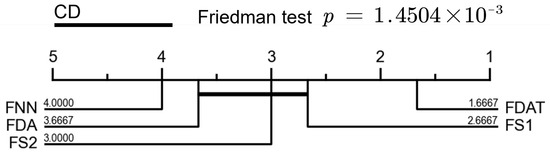
Figure 4.
Statistical significance tests for the learning methods involved in ablation study. Groups of classifiers that are not significantly different (at p = 0.10) will be connected.
5.2. Compared Study Results
We quantitatively compared FDAT with the SA method, which achieves great results through a simple structure and also attempts to perform feature space alignment [45]. Specifically, we tested their performance based on BS, KS, AUC, sensitivity, and specificity when training models with only the source domain data versus using the full target domain labeled data. Table 5 shows the transfer performance of each model when German and Give-credit datasets, both of which are small-scale, are used as the source domains. From the table, it is evident that, when using only source-domain data and a small amount of target-domain unlabeled data, the models outperform the SA-trained models and those trained with only source-domain data in all five evaluation metrics and slightly lag behind models trained directly with target-domain data, which indicates that the models exhibit the best transfer performance on small-scale datasets.In experiments where the German and give-credit datasets are transferred to other datasets, FDAT outperforms the SA model in BS, KS, AUC, sensitivity, and specificity by an average of 0.14, 0.09, 0.03, 0.05, and 0.05, respectively. The BS and KS metrics show particularly significant improvements, highlighting that the FDAT model more accurately reflects customer default probabilities.
Table 5.
Model transfer performance using 2 small-size datasets as source domain.
Furthermore, we used larger datasets such as Chinese and credit-fraud as the source domain, and the results are shown in Table 6. All five indicators show better performance than when small datasets were used as the source domain. Specifically, in the sensitivity metric, which evaluates the ability to recognize default samples, FDAT demonstrates superior performance with large datasets such as Chinese and credit-fraud compared to small datasets. When the data are transferred to credit-fraud, which is an extremely imbalanced dataset with different task objectives, the transfer effect using the large dataset as the source domain is notably better. This suggests that the model is more capable of discriminating between potential defaulters. This improvement may be due to two factors: (1) large datasets contain richer credit behavior patterns and greater diversity, which enhances transfer matching, and (2) large datasets are better at recognizing anomalous samples and long-tailed distributions.
Table 6.
Model transfer performance using 2 large-size datasets as source domain.
As with the methodology used for the ablation part, we performed statistical tests on the results of the comparison study. The results are shown in Figure 5, where the significant difference between FDAT and SA proves the effectiveness of our model in handling different types of credit data.
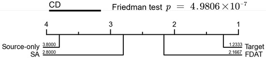
Figure 5.
Statistical significance tests for the learning methods involved in compared study. Groups of classifiers that are not significantly different (at p = 0.10) will be connected.
Finally, we assessed the computational efficiency of the proposed transfer model by summarizing the average computation time. Table 7 shows the average time (in seconds) for the model to train one epoch with a batch size of 64. The results indicate that, despite being more complex than traditional models such as SA, the proposed transfer model maintains a comparable average computation time for both small and large datasets as source domains, thanks to the improvements made by the feature partitioning mechanism. In conclusion, the experimental validation of our proposed method demonstrates superior and more robust performance.
Table 7.
Average computation times for all the used source domain data (in seconds).
5.3. Visualized Analysis
In this section, we first show the loss curves of FDAT and SA to observe their convergence during training. After that, we use the t-SNE method to downscale and visualize the output of the last layer of the feature extractor to show the role of FDAT in constructing the domain-inseparable space. Finally, we compute and visualize the silhouette coefficient of the FDAT-treated samples to further illustrate the ability of FDAT to cope with changes in data distribution.
Figure 6 illustrates the training behavior of the two transfer models, FDAT and SA, using the Chinese dataset. Figure 6a presents the loss function on the original scale, while Figure 6b displays the loss function after transforming the vertical axis into a logarithmic scale. It is evident that FDAT maintains a convergence rate similar to that of SA, even when handling large datasets. This observation aligns with the results presented in Table 7. The feature divider enables the transfer learner and the decision tree to each receive a subset of features, rather than the entire set, thus enhancing the computational efficiency of the fusion model.
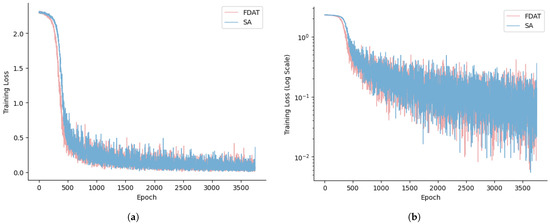
Figure 6.
Loss function behavior of FDAT and SA: (a) standard loss function with the original scale; (b) loss function on a logarithmic scale.
To more visually demonstrate the performance of the FDAT model in the transfer task, we use the t-SNE projection method [46] to visualize the feature distribution of credit scoring data, color-coding the scatter points based on their domains (source or target). When the scatter points of different colors are positioned differently in the plot, it indicates significant distributional shifts between the two types of feature data. Conversely, if the scatter points from different colors are mixed together with no clear boundaries, it suggests that the feature data from the source and target domains are inseparable. This experiment was conducted using the German and Chinese datasets, with the results shown in Figure 7 and Figure 8.
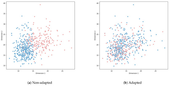
Figure 7.
Give-credit->German: visualization of top feature extractor layer.
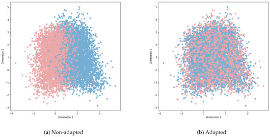
Figure 8.
Credit-fraud->Chinese: visualization of last hidden layer of the label classifier.
In the experiment, we passed the preprocessed data through an FNN (replacing the domain-adversarial transfer module with a BP neural network). The outputs from the feature extractor or the label predictor were used for plotting Figure 7a and Figure 8a, while Figure 7b and Figure 8b show the results after domain adaptation using FDAT. When the credit data are unprocessed, the source and target domains exhibit clear distributional differences, which is visible in the distinct positioning of colored points in the plots. However, after applying FDAT to the credit data, the distinct separation between the domains becomes much less obvious. This further demonstrates the effectiveness of FDAT in reducing domain distribution differences.
Furthermore, Figure 9 shows, in a more numerical way, the values of the silhouette coefficient before and after transfer for credit data. The silhouette coefficient is a metric of the effectiveness of clustering, and it takes values between −1 and 1. For a data sample, the closer its silhouette coefficient is to 1, the better the clustering algorithm works. As for the transfer task, its goal is opposite to that of the clustering algorithm, so we cleverly apply the silhouette coefficient to analyze the effect of FDAT and SA. In Figure 9, the horizontal axis represents the silhouette coefficient of each sample (with each sample corresponding to a line segment), while the vertical axis accumulates all the trained samples, forming the entire silhouette coefficient graph. The red dashed line represents the mean silhouette coefficient of all samples. It can be observed that the data after applying the FDAT model meet the requirement of domain indivisibility, with the mean silhouette coefficient remaining close to 0. In contrast, the effect of SA is slightly less pronounced, further confirming the effectiveness of the FDAT model.
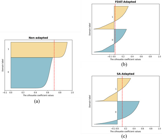
Figure 9.
The silhouette coefficient plot: (a) Non-adapted samples; (b) samples processed by FDAT; (c) samples processed by SA. The brown part represents accepted samples, while the dark blue part represents rejected samples.
6. Explainability Analysis
In the financial sector, explainability of credit scoring models is a critical regulatory requirement. The EU General Data Protection Regulation (GDPR) stipulates that when a bank uses a machine learning model to reject a loan application, it must explain to the applicant how key model factors (e.g., income, debt ratios) influence the assessment results [47]. Similarly, Basel III mandates that organizations using credit scoring models must disclose the weights of key variables and the decision logic to regulators. To gain a deeper understanding of the decision-making process in the FDAT model, we analyze the feature importance using the ex post explainable method, Shapley Additive Explanation [48], which can give us the importance of features. Specifically, the FNN model serves as the base for the FDAT model after eliminating the domain-adversarial transfer module. We compute the Shapley values of the features after training both FDAT and FNN models with identical approaches and datasets, enabling the identification of the most influential features on credit scores in both models. For this analysis, we use the Chinese dataset as the source domain and investigate its transfer to the German dataset. The resulting graph in Figure 10 illustrates the features in the German dataset, ordered by importance, with FNN on the left and FDAT on the right.
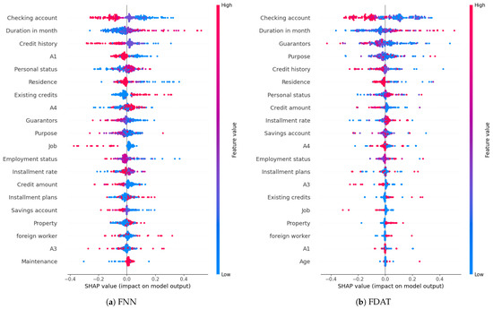
Figure 10.
Beeswarm plot of German dataset based on the features Shapley value.
In terms of feature importance, the existing bank account status (checking account), which serves as the foundation for credit scoring, maintains the greatest influence on predictions both before and after transfer. The increased significance of credit history post-transfer suggests that the German dataset places greater emphasis on individuals’ long-term borrowing behavior, compared to the credit scenarios represented in the Chinese dataset. This shift may be due to the fact that the Chinese dataset originates from internet-based financial institutions, which focus more on the form of guarantees for borrowing and lending. These institutions may offset the hidden risks associated with individuals’ past poor records by relying on guarantor behavior, thereby expanding borrowing and lending. This hypothesis is further supported by the decline in the importance of guarantors after transfer. Notably, transfer leads to a significant drop in the feature importance of the purpose of lending (Purpose), which falls from fourth to tenth place. Considering that the Chinese dataset was collected much later than the data for the German dataset, it is hypothesized that the change in the importance of Purpose may be attributed to shifting perceptions of borrowers’ indebtedness. With the development of the financial industry, some borrowers may take on debt not solely to meet personal needs but to engage in investment activities. Excessive borrowing and investment leverage could negatively impact their credit evaluation [49].
From the relationship between feature values and SHAP values, it can be observed that the impact of the existing bank account status (checking account) on the credit score is more pronounced. Specifically, the inverse relationship between the status value and the predicted value is more apparent, suggesting that FDAT enhances the model’s ability to assess the influence of features through the unlabeled data in the target domain. Similarly, the effects of guarantors, credit history, and installment rate on predicted values are also more significant, indicating that FDAT demonstrates excellent transfer performance.
7. Conclusions
In this study, a fusion modeling framework FDAT based on adversarial transfer learning and feature partitioning is proposed for credit scoring. Through an ablation and comparison study using six commonly used metrics across four credit datasets of varying sizes, the results demonstrate that FDAT improved AUC, sensitivity, and specificity by 4%, 11%, and 2%, respectively, relative to SA, especially when facing distributional shift. It effectively generates a domain-indistinguishable representation of credit data. At the core of FDAT is the decision-making process, which considers the differences in feature distributions between the source and target domains at two points in time. The feature divider first selects features with significant distributional shifts using the Wasserstein distance metric, which ensures that the adversarial transfer learning module can focus on processing features with distributional differences. Then, the adversarial transfer learning module maps both sets of features to the same feature space using a shared mapping function. Finally, a decision tree model is fused to make predictions through weighted voting.
In response to regulatory requirements in the financial sector, we also analyze the model’s explainability. Given that the decision tree component of FDAT is inherently interpretable, we focus on understanding the decision-making process within the adversarial transfer module and explore how domain adaptation affects feature importance. However, it should be noted that we illustrate the ex post explainability of FDAT, and the ex ante explainability for deep models needs to be further explored. When compared to traditional credit scoring methods (decision trees, BP neural networks) and existing transfer techniques (such as SA), FDAT demonstrates clear advantages across datasets of various sizes. This suggests that FDAT could become a promising approach for loan decision-making in financial institutions. By aiding banks and financial organizations in developing advanced internal credit scoring systems, FDAT could significantly enhance both efficiency and profitability.
Despite its strong performance in transfer tasks, the model is still impacted by the challenges posed by extremely unbalanced credit data. Additionally, the interpretability of the adversarial transfer module requires further refinement. Future research directions include exploring improved transfer learning structures for better training efficiency and prediction accuracy; developing methods to handle unbalanced data more effectively; improving generalization performance; and enhancing the adversarial transfer module to maintain transfer performance while improving ex ante interpretability, ensuring compliance with the financial sector’s regulatory needs.
Author Contributions
Methodology, software, writing—original draft preparation, F.X.; writing—review and editing, funding acquisition, R.Z. All authors have read and agreed to the published version of the manuscript.
Funding
This research was funded by the National Natural Science Foundation of China under grant No. 72401144.
Data Availability Statement
We have shared the link to the data in the manuscript.
Conflicts of Interest
The authors declare that they have no known competing financial interests or personal relationships that could have appeared to influence the work reported in this paper.
References
- King, P.; Tarbert, H. Basel III: An overview. Bank. Financ. Serv. Policy Rep. 2011, 30, 1–18. [Google Scholar]
- Kwon, S.; Jang, J.; Kim, C.O. Credit scoring using multi-task Siamese neural network for improving prediction performance and stability. Expert Syst. Appl. 2025, 259, 125327. [Google Scholar]
- Runchi, Z.; Liguo, X.; Qin, W. An ensemble credit scoring model based on logistic regression with heterogeneous balancing and weighting effects. Expert Syst. Appl. 2023, 212, 118732. [Google Scholar]
- Dastile, X.; Celik, T.; Potsane, M. Statistical and machine learning models in credit scoring: A systematic literature survey. Appl. Soft Comput. 2020, 91, 106263. [Google Scholar]
- Fan, C.; Sun, Y.; Zhao, Y.; Song, M.; Wang, J. Deep learning-based feature engineering methods for improved building energy prediction. Appl. Energy 2019, 240, 35–45. [Google Scholar] [CrossRef]
- Xu, Y.; Peng, Z.; Sun, Z.; Zhan, H.; Li, S. Does digital finance lessen credit rationing?—Evidence from Chinese farmers. Res. Int. Bus. Financ. 2022, 62, 101712. [Google Scholar] [CrossRef]
- Xiao, J.; Zhou, X.; Zhong, Y.; Xie, L.; Gu, X.; Liu, D. Cost-sensitive semi-supervised selective ensemble model for customer credit scoring. Knowl.-Based Syst. 2020, 189, 105118. [Google Scholar] [CrossRef]
- Song, H.; Kim, M.; Park, D.; Shin, Y.; Lee, J.G. Learning from noisy labels with deep neural networks: A survey. IEEE Trans. Neural Networks Learn. Syst. 2022, 34, 8135–8153. [Google Scholar]
- Babenko, A.; Slesarev, A.; Chigorin, A.; Lempitsky, V. Neural codes for image retrieval. In Proceedings of the Computer Vision—ECCV 2014: 13th European Conference, Zurich, Switzerland, 6–12 September 2014. [Google Scholar]
- Daume, H., III; Marcu, D. Domain adaptation for statistical classifiers. J. Artif. Intell. Res. 2006, 26, 101–126. [Google Scholar] [CrossRef]
- Bequé, A.; Lessmann, S. Extreme learning machines for credit scoring: An empirical evaluation. Expert Syst. Appl. 2017, 86, 42–53. [Google Scholar]
- Homonoff, T.; O’Brien, R.; Sussman, A.B. Does knowing your fico score change financial behavior? Evidence from a field experiment with student loan borrowers. Rev. Econ. Stat. 2021, 103, 236–250. [Google Scholar] [CrossRef]
- Nikolić, M.; Teodorović, D. Transit network design by bee colony optimization. Expert Syst. Appl. 2013, 40, 5945–5955. [Google Scholar] [CrossRef]
- Sohn, S.Y.; Kim, J.W. Decision tree-based technology credit scoring for start-up firms: Korean case. Expert Syst. Appl. 2012, 39, 4007–4012. [Google Scholar] [CrossRef]
- Forough, J.; Momtazi, S. Ensemble of deep sequential models for credit card fraud detection. Appl. Soft Comput. 2021, 99, 106883. [Google Scholar] [CrossRef]
- Liu, J.; Zhang, S.; Fan, H. A two-stage hybrid credit risk prediction model based on XGBoost and graph-based deep neural network. Expert Syst. Appl. 2022, 195, 116624. [Google Scholar] [CrossRef]
- Dietterich, T.G. Ensemble methods in machine learning. In Proceedings of the International Workshop on Multiple Classifier Systems, Cagliari, Italy, 21–23 June 2000; pp. 1–15. [Google Scholar]
- Shen, F.; Zhao, X.; Kou, G. Three-stage reject inference learning framework for credit scoring using unsupervised transfer learning and three-way decision theory. Decis. Support Syst. 2020, 137, 113366. [Google Scholar] [CrossRef]
- Roseline, J.F.; Naidu, G.; Pandi, V.S.; alias Rajasree, S.A.; Mageswari, N. Autonomous credit card fraud detection using machine learning approach. Comput. Electr. Eng. 2022, 102, 108132. [Google Scholar] [CrossRef]
- Qian, H.; Ma, P.; Gao, S.; Song, Y. Soft reordering one-dimensional convolutional neural network for credit scoring. Knowl.-Based Syst. 2023, 266, 110414. [Google Scholar] [CrossRef]
- Shen, F.; Yang, Z.; Kuang, J.; Zhu, Z. Reject inference in credit scoring based on cost-sensitive learning and joint distribution adaptation method. Expert Syst. Appl. 2024, 251, 124072. [Google Scholar] [CrossRef]
- Pan, S.Q. A survey on transfer learning. IEEE Trans. Knowl. Data Eng. 2010, 22, 1345–1359. [Google Scholar] [CrossRef]
- Banasik, J.; Crook, J. Reject inference, augmentation, and sample selection. Eur. J. Oper. Res. 2007, 183, 1582–1594. [Google Scholar] [CrossRef]
- Li, Z.; Tian, Y.; Li, K.; Zhou, F.; Yang, W. Reject inference in credit scoring using semi-supervised support vector machines. Expert Syst. Appl. 2017, 74, 105–114. [Google Scholar] [CrossRef]
- Kang, Y.; Jia, N.; Cui, R.; Deng, J. A graph-based semi-supervised reject inference framework considering imbalanced data distribution for consumer credit scoring. Appl. Soft Comput. 2021, 105, 107259. [Google Scholar]
- Mancisidor, R.A.; Kampffmeyer, M.; Aas, K.; Jenssen, R. Deep generative models for reject inference in credit scoring. Knowl.-Based Syst. 2020, 196, 105758. [Google Scholar] [CrossRef]
- Xiang, Y.; Zhao, C.; Wei, X.; Lu, Y.; Liu, S. Multi-step Domain Adaption Image Classification Network via Attention Mechanism and Multi-level Feature Alignment. In Proceedings of the Wireless Algorithms, Systems, and Applications: 16th International Conference, WASA 2021, Nanjing, China, 25–27 June 2021; pp. 11–19. [Google Scholar]
- Yao, Y.; Li, X.; Zhang, Y.; Ye, Y. Multisource heterogeneous domain adaptation with conditional weighting adversarial network. IEEE Trans. Neural Netw. Learn. Syst. 2021, 34, 2079–2092. [Google Scholar]
- Gupta, S.; Hoffman, J.; Malik, J. Cross modal distillation for supervision transfer. In Proceedings of the IEEE Conference on Computer Vision and Pattern Recognition, Las Vegas, NV, USA, 27–30 June 2016; pp. 2827–2836. [Google Scholar]
- AghaeiRad, A.; Chen, N.; Ribeiro, B. Improve credit scoring using transfer of learned knowledge from self-organizing map. Neural Comput. Appl. 2017, 28, 1329–1342. [Google Scholar]
- Cortes, C.; Mohri, M. Domain adaptation and sample bias correction theory and algorithm for regression. Theor. Comput. Sci. 2014, 519, 103–126. [Google Scholar]
- Gong, B.; Grauman, K.; Sha, F. Connecting the dots with landmarks: Discriminatively learning domain-invariant features for unsupervised domain adaptation. In Proceedings of the International Conference on Machine Learning. PMLR, Atlanta, GA, USA, 16–21 June 2013; pp. 222–230. [Google Scholar]
- Zhang, X.; Zhuang, Y.; Wang, W.; Pedrycz, W. Online feature transformation learning for cross-domain object category recognition. IEEE Trans. Neural Netw. Learn. Syst. 2017, 29, 2857–2871. [Google Scholar]
- Ajakan, H.; Germain, P.; Larochelle, H.; Laviolette, F.; Marchand, M. Domain-adversarial neural networks. arXiv 2014, arXiv:1412.4446. [Google Scholar]
- Ben-David, S.; Blitzer, J.; Crammer, K.; Pereira, F. Analysis of representations for domain adaptation. Adv. Neural Inf. Process. Syst. 2006, 19, 137–144. [Google Scholar]
- South German Credit. UCI Machine Learning Repository. 2019. Available online: https://archive.ics.uci.edu/dataset/522/south+german+credit (accessed on 10 January 2025).
- Give Me Some Credit. kaggle Database. 2011. Available online: https://www.kaggle.com/c/GiveMeSomeCredit/data (accessed on 10 January 2025).
- Credit Card Fraud Detection. Kaggle Database. 2024. Available online: https://www.kaggle.com/competitions/credit-card-fraud-prediction/data (accessed on 10 January 2025).
- Chinese Credit Datasets. Ali Tianchi Database. 2022. Available online: https://tianchi.aliyun.com/dataset/140861 (accessed on 10 January 2025).
- Řezáč, M.; Řezáč, F. How to measure the quality of credit scoring models. Financ. a úvěr Czech J. Econ. Financ. 2011, 61, 486–507. [Google Scholar]
- Forman, G.; Cohen, I. Beware the null hypothesis: Critical value tables for evaluating classifiers. In Proceedings of the European Conference on Machine Learning, Porto, Portugal, 3–7 October 2005; Springer: Berlin/Heidelberg, Germany, 2005; pp. 133–145. [Google Scholar]
- Blattenberger, G.; Lad, F. Separating the Brier score into calibration and refinement components: A graphical exposition. Am. Stat. 1985, 39, 26–32. [Google Scholar]
- Hand, D.J. Good practice in retail credit scorecard assessment. J. Oper. Res. Soc. 2005, 56, 1109–1117. [Google Scholar]
- Naser, M.; Alavi, A.H. Error metrics and performance fitness indicators for artificial intelligence and machine learning in engineering and sciences. Archit. Struct. Constr. 2023, 3, 499–517. [Google Scholar] [CrossRef]
- Fernando, B.; Habrard, A.; Sebban, M.; Tuytelaars, T. Unsupervised visual domain adaptation using subspace alignment. In Proceedings of the IEEE International Conference on Computer Vision, Sydney, Australia, 1–8 December 2013; pp. 2960–2967. [Google Scholar]
- Van der Maaten, L.; Hinton, G. Visualizing data using t-SNE. J. Mach. Learn. Res. 2008, 9, 2579–2605. [Google Scholar]
- Regulation, P. EU General Data Protection Regulation. 2016. Available online: https://eur-lex.europa.eu/eli/reg/2016/679/oj/ (accessed on 10 September 2023).
- Lundberg, S.M.; Lee, S.I. A unified approach to interpreting model predictions. Adv. Neural Inf. Process. Syst. 2017, 30, 4768–4777. [Google Scholar]
- Lentz, G.; Wang, K. Residential appraisal and the lending process: A survey of issues. J. Real Estate Res. 1998, 15, 11–39. [Google Scholar] [CrossRef]
Disclaimer/Publisher’s Note: The statements, opinions and data contained in all publications are solely those of the individual author(s) and contributor(s) and not of MDPI and/or the editor(s). MDPI and/or the editor(s) disclaim responsibility for any injury to people or property resulting from any ideas, methods, instructions or products referred to in the content. |
© 2025 by the authors. Licensee MDPI, Basel, Switzerland. This article is an open access article distributed under the terms and conditions of the Creative Commons Attribution (CC BY) license (https://creativecommons.org/licenses/by/4.0/).