
Solving the Economic Load Dispatch Problem by Attaining and Refining Knowledge-Based Optimization


Abstract
1. Introduction
- The ARKO algorithm is presented in this study to attain and refine people’s knowledge using information from more knowledgeable people in a society.
- A set of 41 highly complicated test functions of the CEC-2017 and CEC-2022 test suites, three real-life applications, and 11 well-known MAs are employed to examine and compare the performance of the proposed ARKO algorithm.
- The efficiency of ARKO is assessed in terms of its ability to address a highly non-linear and non-convex SELD problem in power engineering.
2. Static Economic Load Dispatch Problem [65]
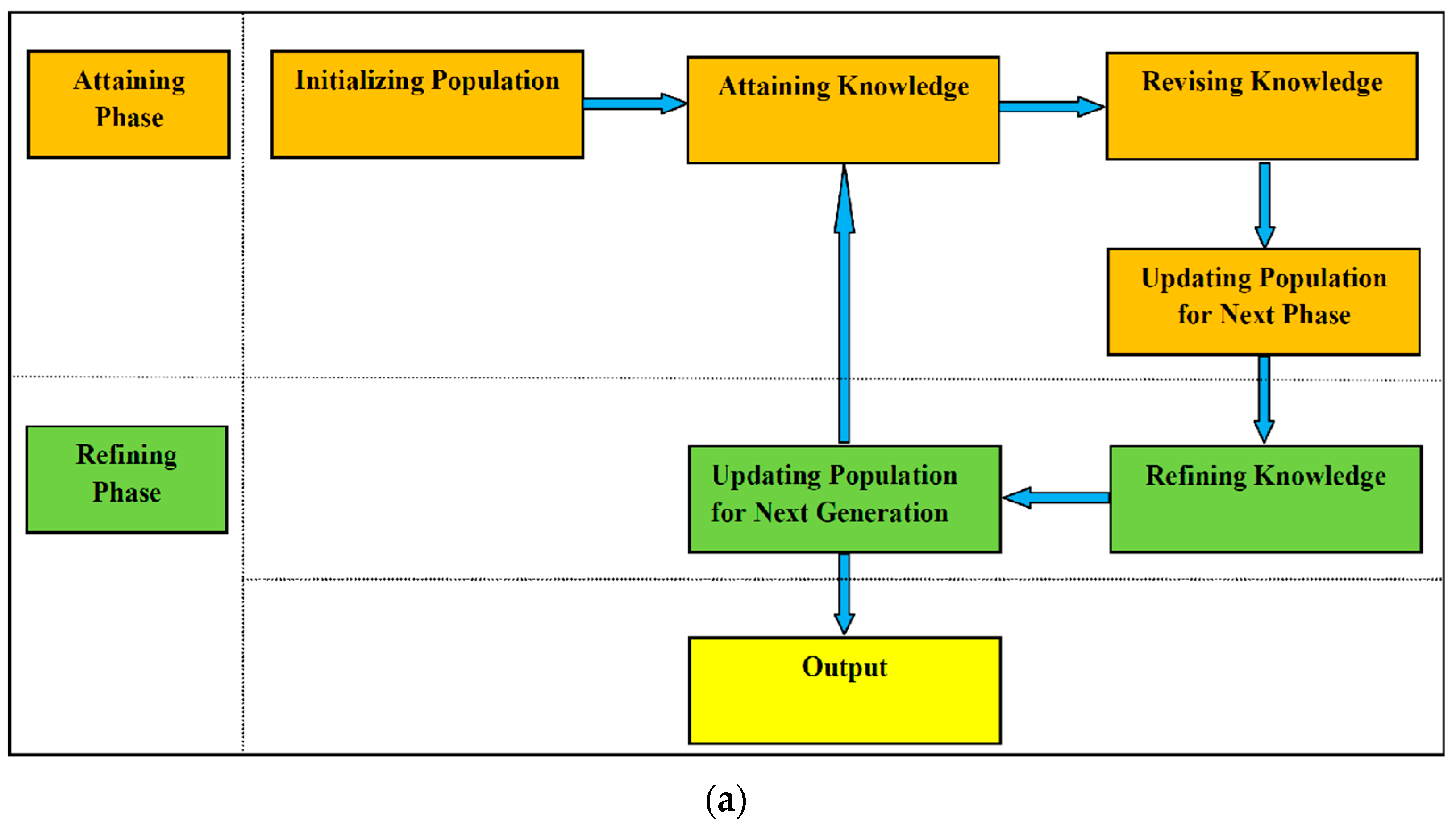
3. Proposed Attaining and Refining Knowledge-Based Optimization (ARKO)
3.1. Inspiration
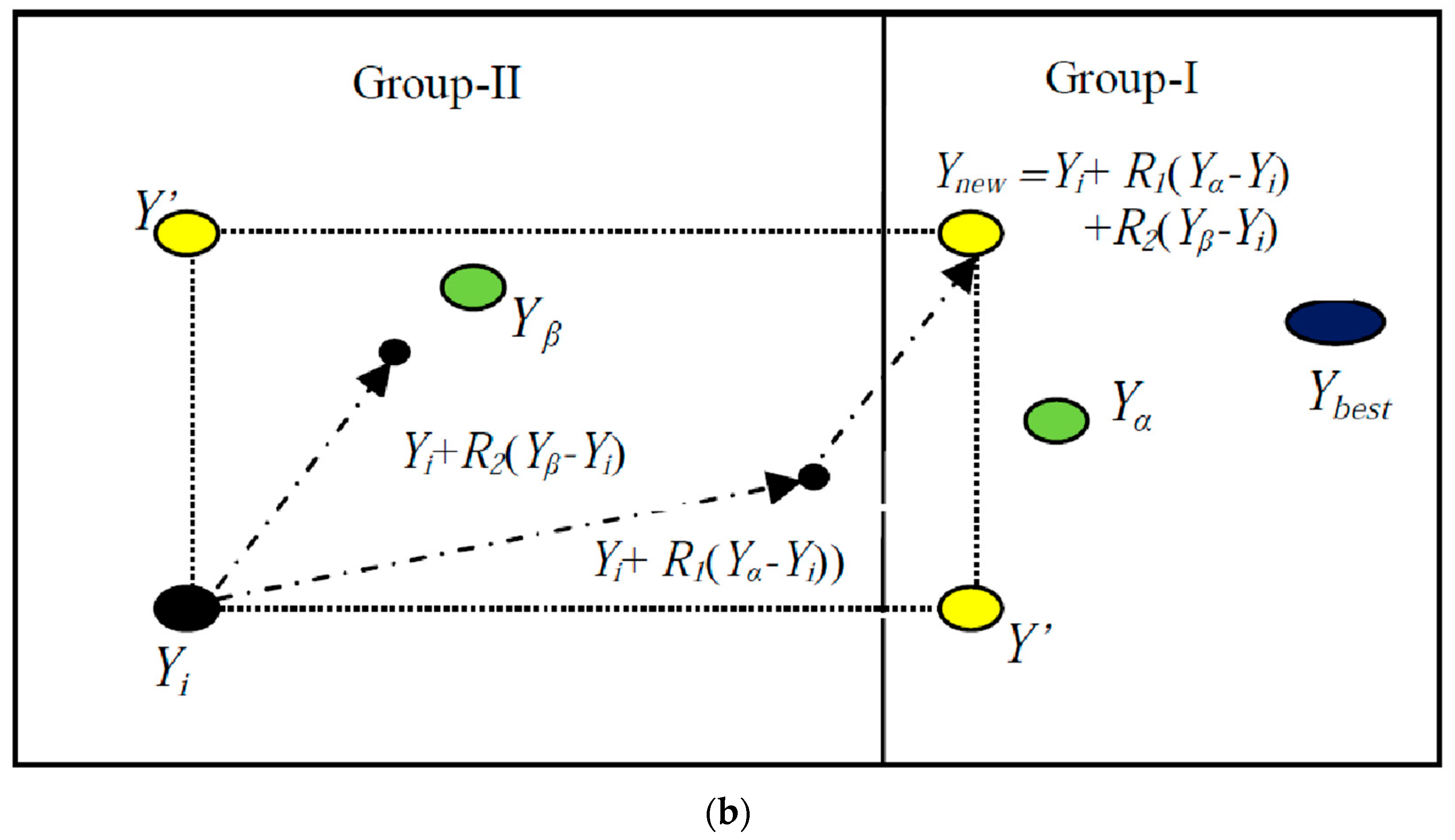
3.2. Mathematical Foundation of ARKO
- Phase-1: Attaining Knowledge
- Phase-2: Refining Knowledge
| Algorithm 1: Attaining and Refining Knowledge-Based Optimization (ARKO) | |
| 1 | Input: M, n, Max-iteration, Mα, TR, ; |
| 2 | Generate initial population using Equation (10); |
| 3 | Calculate function value f(Yi) for each I; |
| 4 | While iteration ≤ Max_Iteration; |
| 5 | Sort population by their fitness; |
| 6 | For i = 1: M //start phase-1; |
| 7 | Select randomly from best Mα candidates (group-I) and randomly from remaining M − Mα candidates (group-II); |
| 8 | Perform the attaining phase and find using Equations (11) and (12); |
| 9 | Find n1 indexes randomly from j = 1, 2, 3,…n and revise using Equation (13): |
| 10 | if : ; else: ; Update population for the second phase using Equation (14); |
| 11 | End For //end phase-1; |
| 12 | For i = 1: M //start phase-2; |
| 13 | Select two candidates, for example, and , randomly from the updated population and refine knowledge of using Equations (15) and (16) |
| //Refine knowledge of | |
| 14 | if : ; else: ; Update population for next generation using Equation (17); |
| 15 | End For //end phase-2; |
| 16 | iteration = iteration +1; |
| 17 | End While. |
3.3. Computational Complexity
4. Results Examination
4.1. Performance Evaluation of IEEE CEC Functions
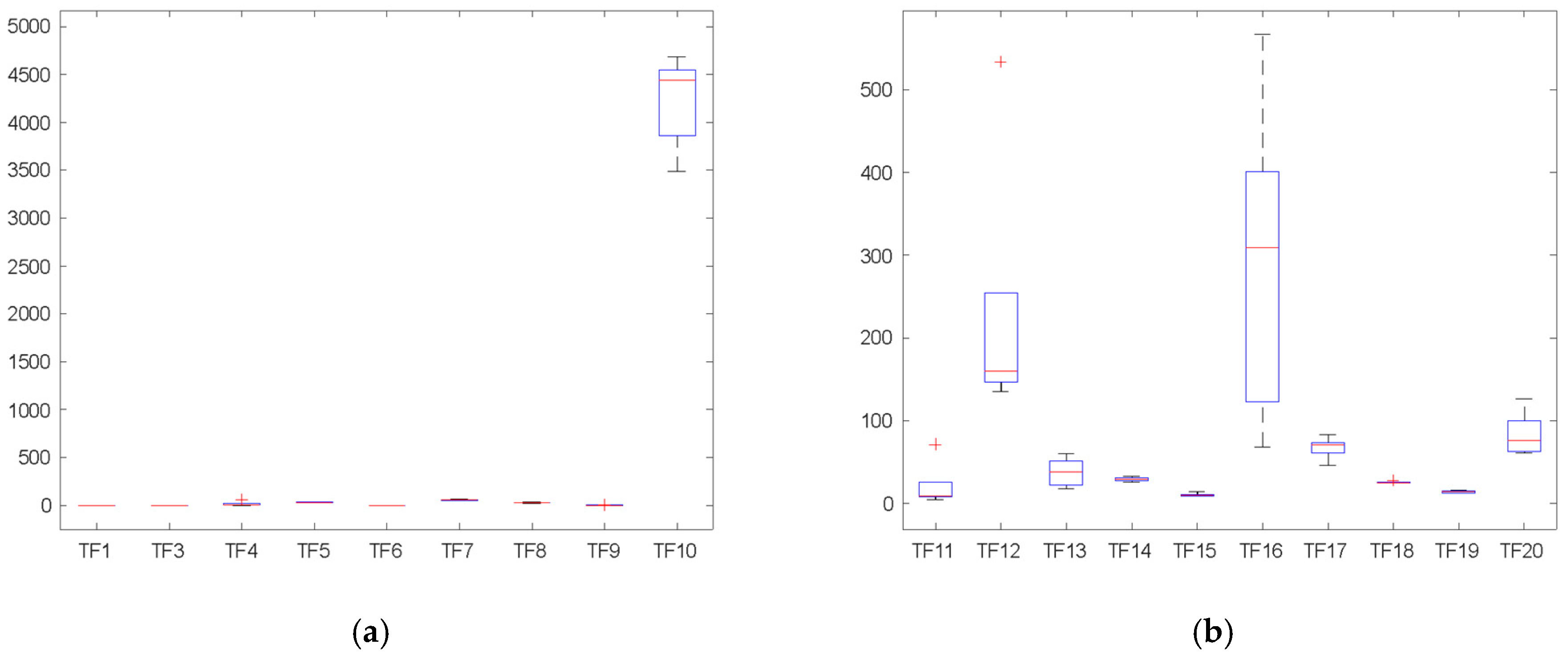
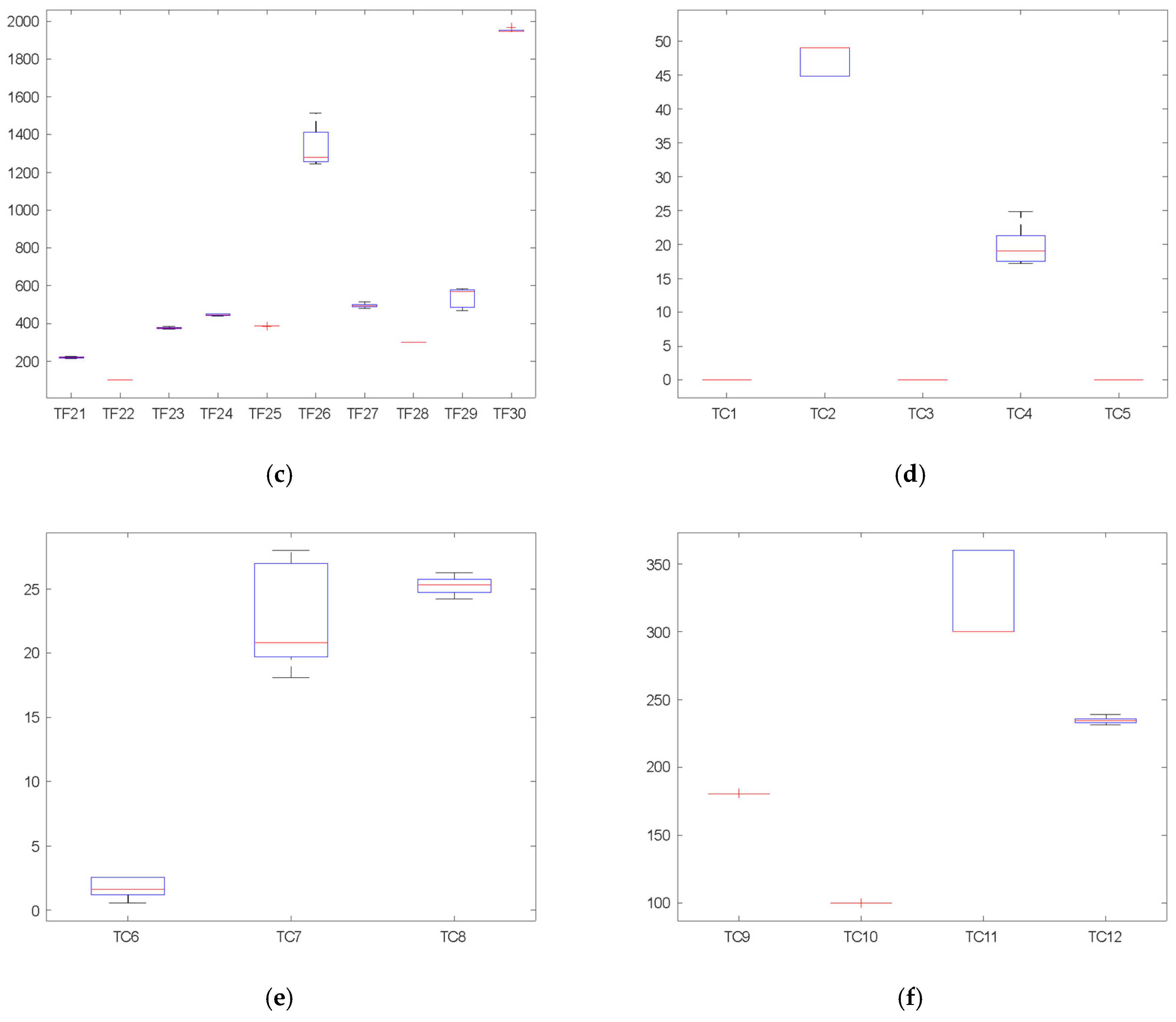
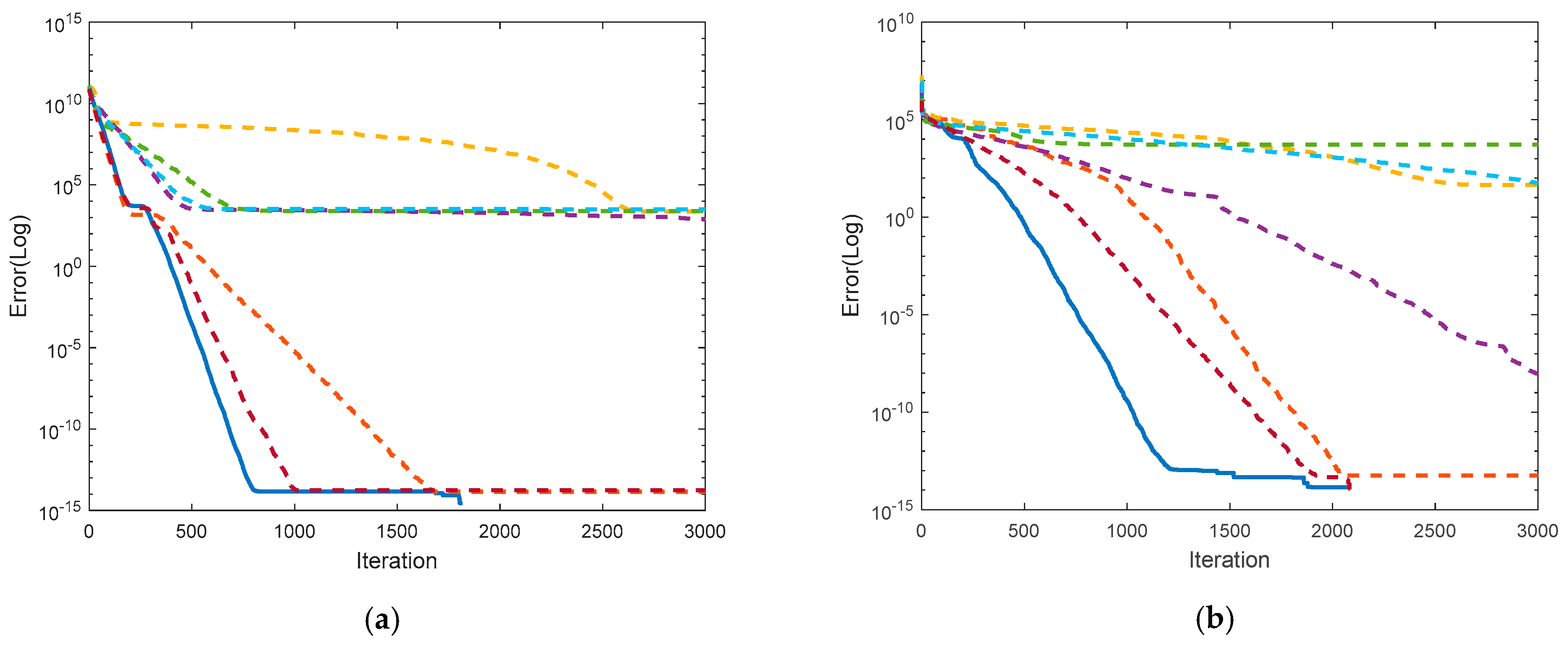
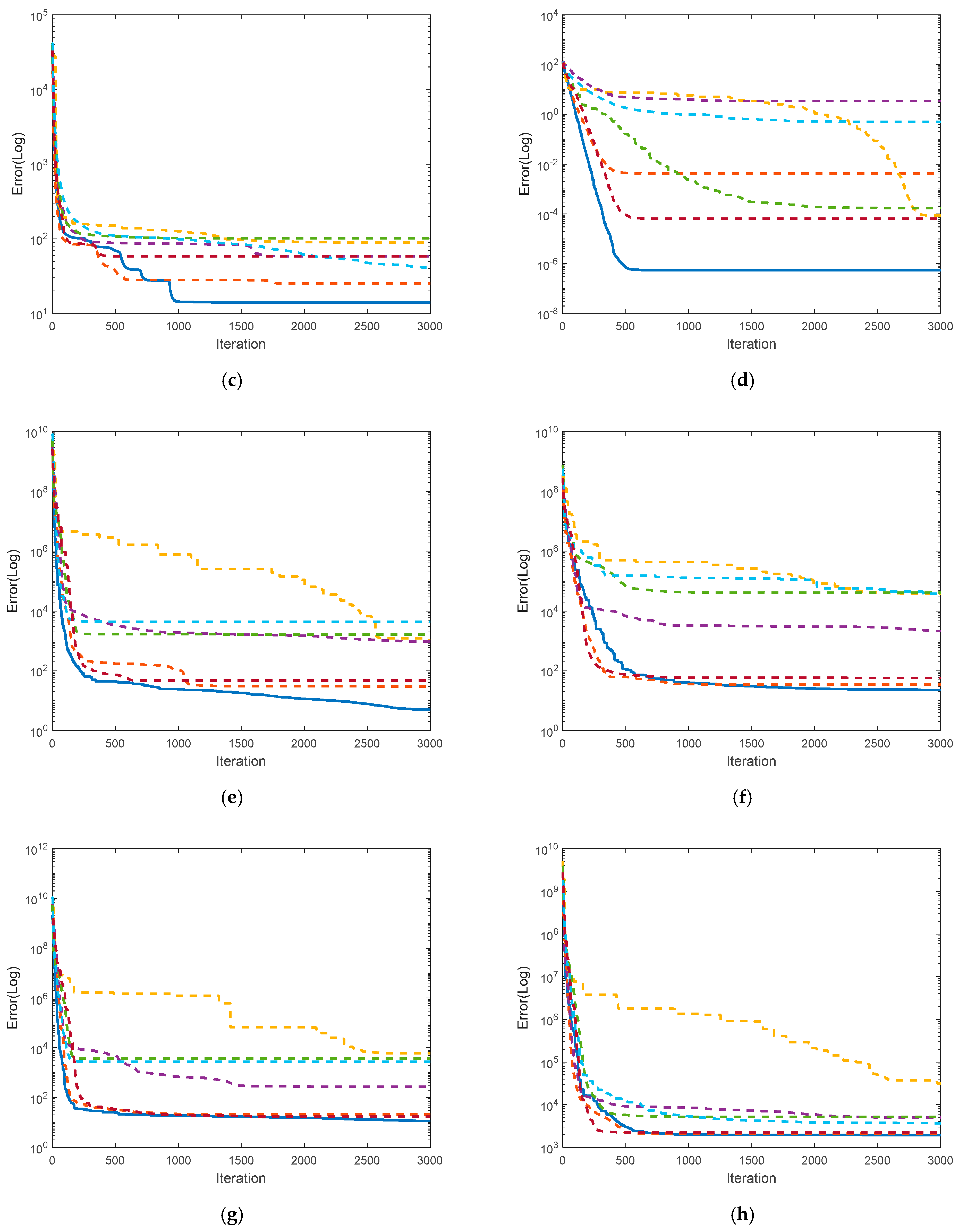
4.1.1. IEEE CEC-2017 Test Functions
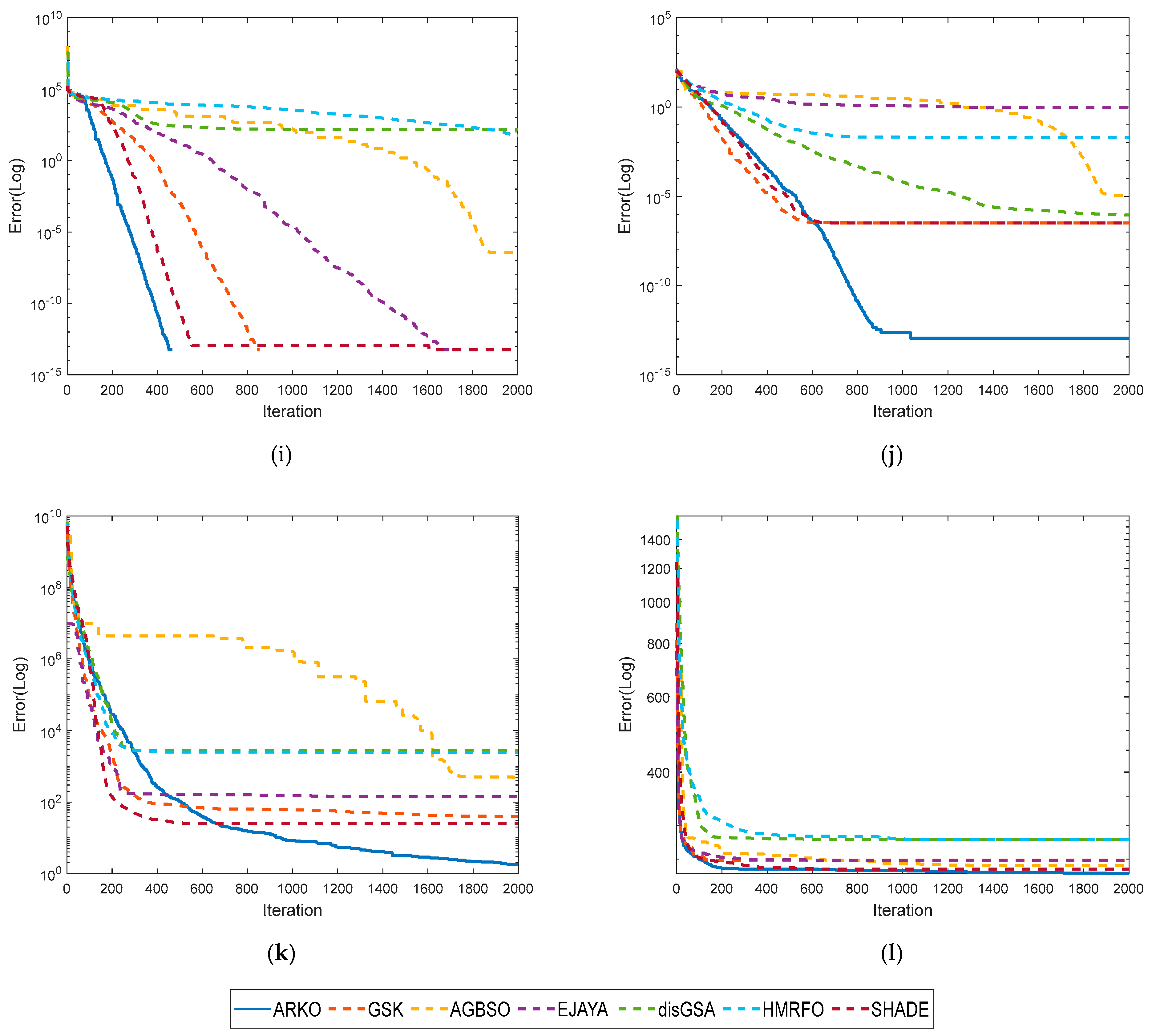
4.1.2. IEEE CEC-2022 Test Functions
4.1.3. Experimental Settings
- System Configuration: OS—Windows 11 (64 bit), processor—i5 (Intel Core 2.6 GHz), and RAM—8 GB.
- M = 100, n = 30, Mα = 20, TR = 0.5, Run = 50, Max-iteration = 100 × n.
4.1.4. Sensitivity Analysis of ARKO on Transfer Ratio
4.1.5. Performance Assessment with Meta-Heuristic Variants
- TLBO [38]: Human-based Meta-heuristics.
- GSK [39]: Human-based Meta-heuristics.
- DTBO [40]: Human-based Meta-heuristics.
- AGBSO [69]: Modified Human-based Meta-heuristics.
- TDSD [70]: (Hybrid Physics-based Meta-heuristics.
- EJaya [71]: Modified EA-based Meta-heuristics.
- DisGSA [72]: Modified Physics-based Meta-heuristics.
- HMRFO [73]: Modified Swarm-based Meta-heuristics.
- CJADE [74]: Modified EA-based Meta-heuristics.
- SHADE [75]: Modified EA-based Meta-heuristics and winner of CEC-2014.
- IMODE [76]: Modified EA-based Meta-heuristics and winner of CEC-2020.
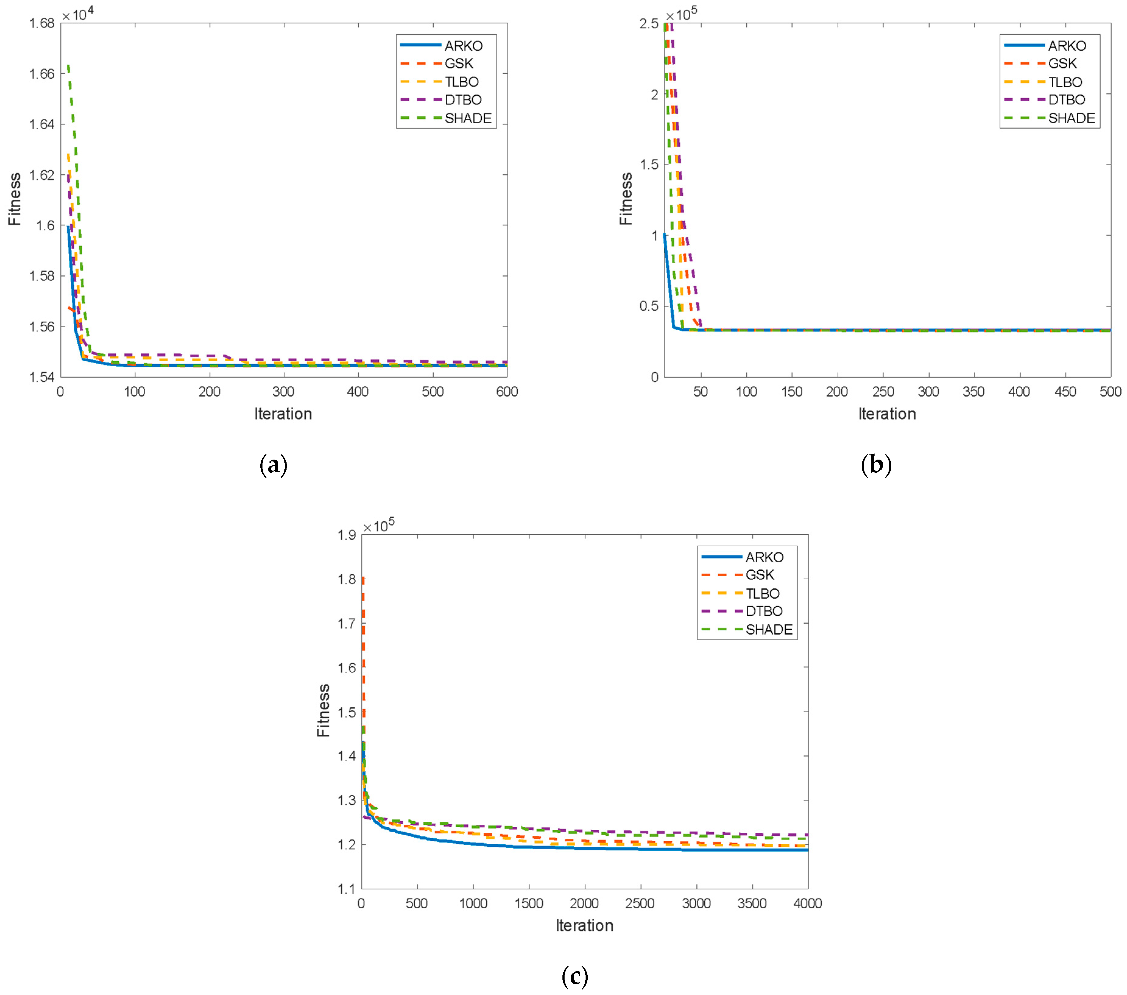
4.2. Performance Evaluation of Real-Life Applications
4.3. Performance Evaluation of ARKO on the SELD Problem
5. Conclusions
Author Contributions
Funding
Data Availability Statement
Conflicts of Interest
References
- Jabr, R.; Coonick, A.; Cory, B. A Homogeneous Linear Programming Algorithm for the Security Constrained Economic Dispatch Problem. IEEE Trans. Power Syst. 2000, 15, 930–936. [Google Scholar] [CrossRef]
- Papageorgiou, L.G.; Fraga, E.S. A Mixed Integer Quadratic Programming Formulation for the Economic Dispatch of Generators with Prohibited Operating Zones. Electr. Power Syst. Res. 2007, 77, 1292–1296. [Google Scholar] [CrossRef]
- Kaur, N.; Singh, I. Economic Dispatch Scheduling Using Classical and Newton Raphson Method. Int. J. Eng. Manag. Res. 2015, 5, 711–716. [Google Scholar]
- Xu, Y.; Zhang, W.; Liu, W. Distributed Dynamic Programming-Based Approach for Economic Dispatch in Smart Grids. IEEE Trans. Ind. Informat. 2014, 11, 166–175. [Google Scholar] [CrossRef]
- Singh, N.; Chakrabarti, T.; Chakrabarti, P.; Margala, M.; Gupta, A.; Praveen, S.P.; Krishnan, S.B.; Unhelkar, B. Novel Heuristic Optimization Technique to Solve Economic Load Dispatch and Economic Emission Load Dispatch Problems. Electronics 2023, 12, 2921. [Google Scholar] [CrossRef]
- Hassan, M.H.; Kamel, S.; Jurado, F.; Desideri, U. Global Optimization of Economic Load Dispatch in Large Scale Power Systems Using an Enhanced Social Network Search Algorithm. Int. J. Electr. Power Energy Syst. 2023, 156, 109719. [Google Scholar] [CrossRef]
- Vent, W. Rechenberg, Ingo, Evolutionsstrategie—Optimierung Technischer Systeme Nach Prinzipien Der Biologischen Evolution. 170 S. Mit 36 Abb. Frommann-Holzboog-Verlag. Stuttgart 1973. Broschiert. Feddes Repert. 1975, 86, 337. [Google Scholar] [CrossRef]
- Holland, J. Adaptation in Natural and Artificial Systems: An Introductory Analysis with Application to Biology Control, and Artificial Intelligence; MIT Press: Cambridge, MA, USA, 1975. [Google Scholar]
- Storn, R.; Price, K. Differential Evolution—A Simple and Efficient Heuristic for Global Optimization over Continuous Spaces. J. Glob. Optim. 1997, 11, 341–359. [Google Scholar] [CrossRef]
- Han, K.-H.; Kim, J.-H. Quantum-Inspired Evolutionary Algorithm for a Class of Combinatorial Optimization. IEEE Trans. Evol. Comput. 2002, 6, 580–593. [Google Scholar] [CrossRef]
- Civicioglu, P. Transforming Geocentric Cartesian Coordinates to Geodetic Coordinates by Using Differential Search Algorithm. Comput. Geosci. 2012, 46, 229–247. [Google Scholar] [CrossRef]
- Civicioglu, P. Backtracking Search Optimization Algorithm for Numerical Optimization Problems. Appl. Math. Comput. 2013, 219, 8121–8144. [Google Scholar] [CrossRef]
- Dorigo, M.; Maniezzo, V.; Colorni, A. Ant System: Optimization by a Colony of Cooperating Agents. IEEE Trans. Syst. Man Cybern. Part B Cybern. 1996, 26, 29–41. [Google Scholar] [CrossRef]
- Kennedy, J.; Eberhart, R. Particle Swarm Optimization. In Proceedings of the IEEE International Conference on Neural Networks, Perth, WA, Australia, 27 November–1 December 1995; Volume IV; pp. 1942–1948. [Google Scholar]
- Passino, K.M. Biomimicry of Bacterial Foraging for Distributed Optimization and Control. IEEE Control Syst. Mag. 2002, 22, 52–67. [Google Scholar] [CrossRef]
- Karaboga, D.; Basturk, B. A Powerful and Efficient Algorithm for Numerical Function Optimization: Artificial Bee Colony (ABC) Algorithm. J. Glob. Optim. 2007, 39, 459–471. [Google Scholar] [CrossRef]
- Yang, X.S.; Deb, S. Cuckoo Search via Lévy Flights. In Proceedings of the 2009 World Congress on Nature and Biologically Inspired Computing, NABIC 2009—Proceedings, Coimbatore, India, 9–11 December 2009. [Google Scholar]
- Yang, X.S. A New Metaheuristic Bat-Inspired Algorithm; Studies in Computational Intelligence; Springer: Berlin, Germany, 2010. [Google Scholar]
- Yang, X.S. Firefly Algorithm, Stochastic Test Functions and Design Optimization. Int. J. Bio-Inspired Comput. 2010, 2, 78. [Google Scholar] [CrossRef]
- Mirjalili, S.; Mirjalili, S.M.; Lewis, A. Grey Wolf Optimizer. Adv. Eng. Softw. 2014, 69, 46–61. [Google Scholar] [CrossRef]
- Mirjalili, S.; Lewis, A. The Whale Optimization Algorithm. Adv. Eng. Softw. 2016, 95, 51–67. [Google Scholar] [CrossRef]
- Zhao, W.; Zhang, Z.; Wang, L. Manta Ray Foraging Optimization: An Effective Bio-Inspired Optimizer for Engineering Applications. Eng. Appl. Artif. Intell. 2020, 87, 103300. [Google Scholar] [CrossRef]
- Abualigah, L.; Elaziz, M.A.; Sumari, P.; Geem, Z.W.; Gandomi, A.H. Reptile Search Algorithm (RSA): A nature-inspired meta-heuristic optimizer. Expert Syst. Appl. 2022, 191, 116158. [Google Scholar] [CrossRef]
- Kirkpatrick, S.; Gelatt, C.D.; Vecchi, M.P. Optimization by Simulated Annealing. Science 1983, 220, 671–680. [Google Scholar] [CrossRef]
- Mladenović, N.; Hansen, P. Variable Neighborhood Search. Comput. Oper. Res. 1998, 24, 1097–1100. [Google Scholar] [CrossRef]
- Geem, Z.W.; Kim, J.H.; Loganathan, G.V. A New Heuristic Optimization Algorithm: Harmony Search. Simulation 2001, 76, 60–68. [Google Scholar] [CrossRef]
- Formato, R.A. Central Force Optimization: A New Metaheuristic with Applications in Applied Electromagnetics. Prog. Electromagn. Res. 2007, 77, 425–491. [Google Scholar] [CrossRef]
- Rashedi, E.; Nezamabadi-Pour, H.; Saryazdi, S. GSA: A Gravitational Search Algorithm. Inf. Sci. 2009, 179, 2232–2248. [Google Scholar] [CrossRef]
- Kaveh, A.; Talatahari, S. A Novel Heuristic Optimization Method: Charged System Search. Acta Mech. 2010, 213, 267–289. [Google Scholar] [CrossRef]
- Hatamlou, A. Black Hole: A New Heuristic Optimization Approach for Data Clustering. Inf. Sci. 2013, 222, 175–184. [Google Scholar] [CrossRef]
- Eskandar, H.; Sadollah, A.; Bahreininejad, A.; Hamdi, M. Water Cycle Algorithm—A Novel Metaheuristic Optimization Method for Solving Constrained Engineering Optimization Problems. Comput. Struct. 2012, 110–111, 151–166. [Google Scholar] [CrossRef]
- Mirjalili, S. SCA: A Sine Cosine Algorithm for Solving Optimization Problems. Knowl.-Based Syst. 2016, 96, 120–133. [Google Scholar] [CrossRef]
- Kaveh, A.; Dadras, A. A Novel Meta-Heuristic Optimization Algorithm: Thermal Exchange Optimization. Adv. Eng. Softw. 2017, 110, 69–84. [Google Scholar] [CrossRef]
- Zhao, W.; Wang, L.; Zhang, Z. A Novel Atom Search Optimization for Dispersion Coefficient Estimation in Groundwater. Futur. Gener. Comput. Syst. 2019, 91, 601–610. [Google Scholar] [CrossRef]
- Ray, T.; Liew, K. Society and Civilization: An Optimization Algorithm Based on the Simulation of Social Behavior. IEEE Trans. Evol. Comput. 2003, 7, 386–396. [Google Scholar] [CrossRef]
- Kashan, A.H. League Championship Algorithm: A New Algorithm for Numerical Function Optimization. In Proceedings of the SoCPaR 2009—Soft Computing and Pattern Recognition, Malacca, Malaysia, 4–7 December 2009. [Google Scholar]
- Shi, Y. Brain Storm Optimization Algorithm. In Lecture Notes in Computer Science (Including subseries Lecture Notes in Artificial Intelligence and Lecture Notes in Bioinformatics); Springer: Berlin/Heidelberg, Germany, 2011. [Google Scholar]
- Rao, R.V.; Savsani, V.J.; Vakharia, D.P. Teaching–Learning-Based Optimization: A Novel Method for Constrained Mechanical Design Optimization Problems. Comput. Aided Des. 2011, 43, 303–315. [Google Scholar] [CrossRef]
- Mohamed, A.W.; Hadi, A.A.; Mohamed, A.K. Gaining-Sharing Knowledge Based Algorithm for Solving Optimization Problems: A Novel Nature-Inspired Algorithm. Int. J. Mach. Learn. Cybern. 2019, 11, 1501–1529. [Google Scholar] [CrossRef]
- Dehghani, M.; Trojovská, E.; Trojovský, P. A New Human-Based Metaheuristic Algorithm for Solving Optimization Problems on the Base of Simulation of Driving Training Process. Sci. Rep. 2022, 12, 9924. [Google Scholar] [CrossRef]
- Walters, D.C.; Sheble, G.B. Genetic Algorithm Solution of Economic Dispatch with Valve Point Loading. IEEE Trans. Power Syst. 1993, 8, 1325–1332. [Google Scholar] [CrossRef]
- Sinha, N.; Chakrabarti, R.; Chattopadhyay, P.K. Evolutionary Programming Techniques for Economic Load Dispatch. IEEE Trans. Evol. Comput. 2003, 7, 83–94. [Google Scholar] [CrossRef]
- Gaing, Z.-L. Particle Swarm Optimization to Solving the Economic Dispatch Considering the Generator Constraints. IEEE Trans. Power Syst. 2003, 18, 1187–1195. [Google Scholar] [CrossRef]
- Noman, N.; Iba, H. Differential Evolution for Economic Load Dispatch Problems. Electr. Power Syst. Res. 2008, 78, 1322–1331. [Google Scholar] [CrossRef]
- Kumar, P.; Pant, M. Modified Random Localisation-Based de for Static Economic Power Dispatch with Generator Constraints. Int. J. Bio-Inspired Comput. 2014, 6, 250. [Google Scholar] [CrossRef]
- Bulbul, S.M.A.; Pradhan, M.; Roy, P.K.; Pal, T. Opposition-Based Krill Herd Algorithm Applied to Economic Load Dispatch Problem. Ain Shams Eng. J. 2016, 9, 423–440. [Google Scholar] [CrossRef]
- Joshi, P.M.; Verma, H.K. An Improved TLBO Based Economic Dispatch of Power Generation through Distributed Energy Resources Considering Environmental Constraints. Sustain. Energy Grids Netw. 2019, 18, 100207. [Google Scholar] [CrossRef]
- Nguyen, H.D.; Pham, L.H. Solutions of Economic Load Dispatch Problems for Hybrid Power Plants Using Dandelion Optimizer. Bull. Electr. Eng. Informat. 2023, 12, 2569–2576. [Google Scholar] [CrossRef]
- Tai, T.-C.; Lee, C.-C.; Kuo, C.-C. A Hybrid Grey Wolf Optimization Algorithm Using Robust Learning Mechanism for Large Scale Economic Load Dispatch with Vale-Point Effect. Appl. Sci. 2023, 13, 2727. [Google Scholar] [CrossRef]
- Wang, X.; Chu, S.C.; Snášel, V.; Shehadeh, H.A.; Pan, J.S. Five Phases Algorithm: A Novel Meta-Heuristic Algorithm and Its Application on Economic Load Dispatch Problem. J. Internet Technol. 2023, 24, 837–848. [Google Scholar] [CrossRef]
- Jain, A.K.; Gidwani, L. Dynamic Economic Load Dispatch in Microgrid Using Hybrid Moth-Flame Optimization Algorithm. Electr. Eng. 2024, 106, 3721–3741. [Google Scholar] [CrossRef]
- Shaban, A.E.; Ismaeel, A.A.K.; Farhan, A.; Said, M.; El-Rifaie, A.M. Growth Optimizer Algorithm for Economic Load Dispatch Problem: Analysis and Evaluation. Processes 2024, 12, 2593. [Google Scholar] [CrossRef]
- Ragunathan, R.; Ramadoss, B. Golden Jackal Optimization for Economic Load Dispatch Problems with Complex Constraints. Bull. Electr. Eng. Informat. 2024, 13, 781–793. [Google Scholar] [CrossRef]
- Wadood, A.; Ghani, A. An Application of Gorilla Troops Optimizer in Solving the Problem of Economic Load Dispatch Considering Valve Point Loading Effect. Eng. Res. Express 2024, 6, 015310. [Google Scholar] [CrossRef]
- Zhang, Y.; Li, H. Research on Economic Load Dispatch Problem of Microgrid Based on an Improved Pelican Optimization Algorithm. Biomimetics 2024, 9, 277. [Google Scholar] [CrossRef]
- Yu, J.-T.; Kim, C.-H.; Wadood, A.; Khurshaid, T.; Rhee, S.-B. Jaya Algorithm with Self-Adaptive Multi-Population and Lévy Flights for Solving Economic Load Dispatch Problems. IEEE Access 2019, 7, 21372–21384. [Google Scholar] [CrossRef]
- Ellahi, M.; Abbas, G. A Hybrid Metaheuristic Approach for the Solution of Renewables-Incorporated Economic Dispatch Problems. IEEE Access 2020, 8, 127608–127621. [Google Scholar] [CrossRef]
- Deb, S.; Houssein, E.H.; Said, M.; Abdelminaam, D.S. Performance of Turbulent Flow of Water Optimization on Economic Load Dispatch Problem. IEEE Access 2021, 9, 77882–77893. [Google Scholar] [CrossRef]
- Said, M.; El-Rifaie, A.M.; Tolba, M.A.; Houssein, E.H.; Deb, S. An Efficient Chameleon Swarm Algorithm for Economic Load Dispatch Problem. Mathematics 2021, 9, 2770. [Google Scholar] [CrossRef]
- Said, M.; Houssein, E.H.; Deb, S.; Ghoniem, R.M.; Elsayed, A.G. Economic Load Dispatch Problem Based on Search and Rescue Optimization Algorithm. IEEE Access 2022, 10, 47109–47123. [Google Scholar] [CrossRef]
- Al-Betar, M.A.; Awadallah, M.A.; Makhadmeh, S.N.; Doush, I.A.; Zitar, R.A.; Alshathri, S.; Abd Elaziz, M. A Hybrid Harris Hawks Optimizer for Economic Load Dispatch Problems. Alex. Eng. J. 2022, 64, 365–389. [Google Scholar] [CrossRef]
- Braik, M.S.; Awadallah, M.A.; Al-Betar, M.A.; Hammouri, A.I.; Zitar, R.A. A Non-Convex Economic Load Dispatch Problem Using Chameleon Swarm Algorithm with Roulette Wheel and Levy Flight Methods. Appl. Intell. 2023, 53, 17508–17547. [Google Scholar] [CrossRef]
- Ismaeel, A.A.K.; Houssein, E.H.; Khafaga, D.S.; Abdullah Aldakheel, E.; AbdElrazek, A.S.; Said, M. Performance of Osprey Optimization Algorithm for Solving Economic Load Dispatch Problem. Mathematics 2023, 11, 4107. [Google Scholar] [CrossRef]
- Wolpert, D.H.; Macready, W.G. No Free Lunch Theorems for Optimization. IEEE Trans. Evol. Comput. 1997, 1, 67–82. [Google Scholar] [CrossRef]
- Das, S.; Suganthan, P.N. Problem Definitions and Evaluation Criteria for CEC 2011 Competition on Testing Evolutionary Algorithms on Real World Optimization Problems; Technical Report; Nanyang Technological University: Kolkata, India, 2011. [Google Scholar]
- Kumar, P.; Ali, M. Improved Differential Evolution Algorithm Guided by Best and Worst Positions Exploration Dynamics. Biomimetics 2024, 9, 119. [Google Scholar] [CrossRef]
- Awad, N.H.; Ali, M.Z.; Liang, J.J.; Qu, B.Y.; Suganthan, P.N. Problem Definitions and Evaluation Criteria for the CEC 2017 Special Session and Competition on Single Objective Bound Constrained Real-Parameter Numerical Optimization; Technical Report; Nanyang Technological University: Singapore, 2016; pp. 1–34. [Google Scholar]
- Kumar, A.; Price, K.V.; Mohamed, A.W.; Hadi, A.A. , Suganthan, P.N. Problem Definitions and Evaluation Criteria for the 2022 Special Session and Competition on Single Objective Bound Constrained Numerical Optimization; Technical Report; Nanyang Technological University: Singapore, 2021. [Google Scholar]
- Peng, Y.; Shen, Z.; Wang, S. Adaptive Grouping Brain Storm Optimization for Multimodal Optimization Problems. Int. J. Swarm Intell. Res. 2021, 12, 81–100. [Google Scholar] [CrossRef]
- Li, X.; Cai, Z.; Wang, Y.; Todo, Y.; Cheng, J.; Gao, S. TDSD: A New Evolutionary Algorithm Based on Triple Distinct Search Dynamics. IEEE Access 2020, 8, 76752–76764. [Google Scholar] [CrossRef]
- Zhang, Y.; Chi, A.; Mirjalili, S. Enhanced Jaya Algorithm: A Simple but Efficient Optimization Method for Constrained Engineering Design Problems. Knowl.-Based Syst. 2021, 233, 107555. [Google Scholar] [CrossRef]
- Guo, A.; Wang, Y.; Guo, L.; Zhang, R.; Yu, Y.; Gao, S. An Adaptive Position-Guided Gravitational Search Algorithm for Function Optimization and Image Threshold Segmentation. Eng. Appl. Artif. Intell. 2023, 121, 106040. [Google Scholar] [CrossRef]
- Tang, Z.; Wang, K.; Tao, S.; Todo, Y.; Wang, R.-L.; Gao, S. Hierarchical Manta Ray Foraging Optimization with Weighted Fitness-Distance Balance Selection. Int. J. Comput. Intell. Syst. 2023, 16, 114. [Google Scholar] [CrossRef]
- Gao, S.; Yu, Y.; Wang, Y.; Wang, J.; Cheng, J.; Zhou, M. Chaotic Local Search-Based Differential Evolution Algorithms for Optimization. IEEE Trans. Syst. Man Cybern. Syst. 2019, 51, 3954–3967. [Google Scholar] [CrossRef]
- Tanabe, R.; Fukunaga, A. Success-History Based Parameter Adaptation for Differential Evolution. In Proceedings of the 2013 IEEE Congress on Evolutionary Computation, Cancun, Mexico, 20–23 June 2013. [Google Scholar] [CrossRef]
- Sallam, K.M.; Elsayed, S.M.; Chakrabortty, R.K.; Ryan, M.J. Improved Multi-Operator Differential Evolution Algorithm for Solving Unconstrained Problems. In Proceedings of the 2020 IEEE Congress on Evolutionary Computation, Glasgow, UK, 9–24 July 2020. [Google Scholar] [CrossRef]


| Fun | TR = 0.3 | TR = 0.5 | TR = 0.7 | TR = 0.9 | ||||||||
|---|---|---|---|---|---|---|---|---|---|---|---|---|
| Best | Mean | SD | Best | Mean | SD | Best | Mean | SD | Best | Mean | SD | |
| tf01 | 0.000 × 100 | 0.000 × 100 | 0.000 × 100 | 0.000 × 100 | 0.000 × 100 | 0.000 × 100 | 0.000 × 100 | 0.000 × 100 | 0.000 × 100 | 0.000 × 100 | 0.000 × 100 | 0.000 × 100 |
| tf03 | 0.000 × 100 | 0.000 × 100 | 0.000 × 100 | 0.000 × 100 | 0.000 × 100 | 0.000 × 100 | 0.000 × 100 | 0.000 × 100 | 0.000 × 100 | 0.000 × 100 | 0.000 × 100 | 0.000 × 100 |
| tf04 | 0.000 × 100 | 0.000 × 100 | 0.000 × 100 | 0.000 × 100 | 0.000 × 100 | 0.000 × 100 | 0.000 × 100 | 0.000 × 100 | 0.000 × 100 | 0.000 × 100 | 0.000 × 100 | 0.000 × 100 |
| tf05 | 9.950 × 10⁻¹ | 2.776 × 100 | 1.389 × 100 | 5.240 × 10⁻⁸ | 1.064 × 100 | 1.254 × 100 | 3.256 × 100 | 4.512 × 100 | 1.328 × 100 | 3.625 × 100 | 4.467 × 100 | 1.010 × 100 |
| tf06 | 0.000 × 100 | 6.821 × 10⁻¹⁴ | 6.227 × 10⁻¹⁴ | 0.000 × 100 | 4.547 × 10⁻¹⁴ | 6.227 × 10⁻¹⁴ | 0.000 × 100 | 9.095 × 10⁻¹⁴ | 5.084 × 10⁻¹⁴ | 1.091 × 10⁻¹¹ | 1.476 × 10⁻¹⁰ | 2.474 × 10⁻¹⁰ |
| tf07 | 1.364 × 101 | 1.485 × 101 | 1.158 × 100 | 1.205 × 101 | 1.378 × 101 | 1.150 × 100 | 1.188 × 101 | 1.451 × 101 | 2.013 × 100 | 1.344 × 101 | 1.651 × 101 | 1.943 × 100 |
| tf08 | 1.536 × 100 | 3.733 × 100 | 1.379 × 100 | 1.009 × 100 | 2.110 × 100 | 1.283 × 100 | 2.700 × 100 | 4.128 × 100 | 1.025 × 100 | 4.134 × 100 | 6.110 × 100 | 2.461 × 100 |
| tf09 | 0.000 × 100 | 0.000 × 100 | 0.000 × 100 | 0.000 × 100 | 0.000 × 100 | 0.000 × 100 | 0.000 × 100 | 0.000 × 100 | 0.000 × 100 | 0.000 × 100 | 0.000 × 100 | 0.000 × 100 |
| tf10 | 1.904 × 10² | 3.641 × 10² | 1.105 × 10² | 1.078 × 10² | 2.938 × 10² | 1.101 × 10² | 1.321 × 10² | 2.526 × 10² | 8.402 × 101 | 1.608 × 10² | 2.373 × 10² | 6.343 × 101 |
| tf11 | 4.027 × 10⁻⁹ | 1.473 × 10⁻⁴ | 2.990 × 10⁻⁴ | 0.000 × 100 | 0.000 × 100 | 0.000 × 100 | 3.829 × 10⁻³ | 3.077 × 10⁻¹ | 2.307 × 10⁻¹ | 1.400 × 10⁻¹ | 7.073 × 10⁻¹ | 5.013 × 10⁻¹ |
| tf12 | 1.140 × 101 | 2.442 × 101 | 1.173 × 101 | 2.550 × 100 | 6.082 × 100 | 4.183 × 100 | 3.978 × 100 | 1.629 × 101 | 7.505 × 100 | 1.105 × 101 | 1.798 × 101 | 7.661 × 100 |
| tf13 | 3.587 × 100 | 5.087 × 100 | 1.101 × 100 | 3.801 × 100 | 4.940 × 100 | 9.225 × 10⁻¹ | 3.443 × 100 | 4.507 × 100 | 7.370 × 10⁻¹ | 2.564 × 100 | 5.270 × 100 | 1.791 × 100 |
| tf14 | 1.293 × 10⁻⁸ | 5.229 × 10⁻² | 5.332 × 10⁻² | 0.000 × 100 | 3.980 × 10⁻¹ | 5.450 × 10⁻¹ | 8.738 × 10⁻⁴ | 2.710 × 10⁻² | 2.149 × 10⁻² | 8.962 × 10⁻² | 5.753 × 10⁻¹ | 4.120 × 10⁻¹ |
| tf15 | 3.188 × 10⁻² | 5.028 × 10⁻² | 1.332 × 10⁻² | 7.559 × 10⁻³ | 1.198 × 10⁻² | 4.309 × 10⁻³ | 5.542 × 10⁻² | 9.599 × 10⁻² | 3.672 × 10⁻² | 9.162 × 10⁻² | 2.883 × 10⁻¹ | 1.668 × 10⁻¹ |
| tf16 | 7.712 × 10⁻¹ | 1.089 × 100 | 3.019 × 10⁻¹ | 2.340 × 10⁻¹ | 7.041 × 10⁻¹ | 4.234 × 10⁻¹ | 1.251 × 100 | 1.554 × 100 | 2.706 × 10⁻¹ | 1.448 × 100 | 1.918 × 100 | 3.553 × 10⁻¹ |
| tf17 | 3.568 × 100 | 1.067 × 101 | 5.720 × 100 | 1.970 × 10⁻¹ | 7.573 × 100 | 9.386 × 100 | 4.093 × 100 | 5.925 × 100 | 1.473 × 100 | 1.695 × 100 | 3.562 × 100 | 1.699 × 100 |
| tf18 | 7.787 × 10⁻³ | 1.527 × 10⁻² | 7.470 × 10⁻³ | 7.312 × 10⁻³ | 3.673 × 10⁻² | 6.393 × 10⁻² | 1.845 × 10⁻² | 3.918 × 10⁻² | 2.627 × 10⁻² | 2.256 × 10⁻¹ | 3.568 × 10⁻¹ | 1.301 × 10⁻¹ |
| tf19 | 5.690 × 10⁻⁴ | 1.945 × 10⁻² | 2.381 × 10⁻² | 8.322 × 10⁻¹⁰ | 3.182 × 10⁻² | 3.295 × 10⁻² | 3.137 × 10⁻² | 8.594 × 10⁻² | 3.317 × 10⁻² | 2.586 × 10⁻¹ | 3.000 × 10⁻¹ | 3.643 × 10⁻² |
| tf20 | 0.000 × 100 | 0.000 × 100 | 0.000 × 100 | 0.000 × 100 | 6.243 × 10⁻² | 1.396 × 10⁻¹ | 0.000 × 100 | 4.320 × 10⁻¹² | 9.533 × 10⁻¹² | 4.279 × 10⁻³ | 4.459 × 10⁻² | 2.446 × 10⁻² |
| tf21 | 1.000 × 10² | 1.000 × 10² | 2.491 × 10⁻¹³ | 1.000 × 10² | 1.416 × 10² | 5.693 × 101 | 1.000 × 10² | 1.000 × 10² | 0.000 × 100 | 1.000 × 10² | 1.000 × 10² | 1.415 × 10⁻³ |
| tf22 | 0.000 × 100 | 7.892 × 101 | 4.418 × 101 | 1.000 × 10² | 1.000 × 10² | 7.007 × 10⁻² | 4.547 × 10⁻¹³ | 6.524 × 101 | 4.849 × 101 | 4.729 × 10⁻¹¹ | 2.004 × 101 | 4.471 × 101 |
| tf23 | 3.046 × 10² | 3.058 × 10² | 1.544 × 100 | 3.000 × 10² | 3.025 × 10² | 1.871 × 100 | 3.048 × 10² | 3.064 × 10² | 9.573 × 10⁻¹ | 3.054 × 10² | 3.075 × 10² | 1.470 × 100 |
| tf24 | 1.000 × 10² | 2.398 × 10² | 1.277 × 10² | 3.252 × 10² | 3.289 × 10² | 3.175 × 100 | 1.000 × 10² | 1.000 × 10² | 0.000 × 100 | 1.000 × 10² | 1.214 × 10² | 4.777 × 101 |
| tf25 | 3.977 × 10² | 3.979 × 10² | 1.541 × 10⁻¹ | 3.980 × 10² | 4.167 × 10² | 2.552 × 101 | 3.977 × 10² | 3.977 × 10² | 0.000 × 100 | 3.977 × 10² | 3.977 × 10² | 5.617 × 10⁻⁵ |
| tf26 | 3.000 × 10² | 3.000 × 10² | 0.000 × 100 | 3.000 × 10² | 3.000 × 10² | 0.000 × 100 | 3.000 × 10² | 3.000 × 10² | 0.000 × 100 | 5.139 × 10⁻¹¹ | 2.400 × 10² | 1.342 × 10² |
| tf27 | 3.890 × 10² | 3.892 × 10² | 2.807 × 10⁻¹ | 3.890 × 10² | 3.894 × 10² | 2.599 × 10⁻¹ | 3.873 × 10² | 3.886 × 10² | 7.283 × 10⁻¹ | 3.869 × 10² | 3.873 × 10² | 9.341 × 10⁻¹ |
| tf28 | 3.000 × 10² | 3.000 × 10² | 0.000 × 100 | 3.000 × 10² | 3.817 × 10² | 1.353 × 10² | 3.000 × 10² | 3.000 × 10² | 0.000 × 100 | 3.000 × 10² | 3.000 × 10² | 0.000 × 100 |
| tf29 | 2.428 × 10² | 2.496 × 10² | 7.520 × 100 | 2.377 × 10² | 2.419 × 10² | 3.838 × 100 | 2.362 × 10² | 2.411 × 10² | 4.346 × 100 | 2.400 × 10² | 2.434 × 10² | 2.385 × 100 |
| tf30 | 3.949 × 10² | 3.950 × 10² | 8.423 × 10⁻² | 3.948 × 10² | 3.950 × 10² | 9.876 × 10⁻² | 3.950 × 10² | 3.952 × 10² | 1.491 × 10⁻¹ | 3.946 × 10² | 3.949 × 10² | 1.750 × 10⁻¹ |
| 1/2/3/4 | 9/9/7/4 | 12/7/3/7 | 13/7/7/2 | 11/2/5/11 | ||||||||
| Rank | 2.21 | 2.17 | 1.97 | 2.55 | ||||||||
| Fun | TR = 0.3 | TR = 0.5 | TR = 0.7 | TR = 0.9 | ||||||||
|---|---|---|---|---|---|---|---|---|---|---|---|---|
| Best | Mean | SD | Best | Mean | SD | Best | Mean | SD | Best | Mean | SD | |
| tf01 | 0.000 × 100 | 0.000 × 100 | 0.000 × 100 | 0.000 × 100 | 0.000 × 100 | 0.000 × 100 | 0.000 × 100 | 0.000 × 100 | 0.000 × 100 | 0.000 × 100 | 0.000 × 100 | 0.000 × 100 |
| tf03 | 0.000 × 100 | 0.000 × 100 | 0.000 × 100 | 0.000 × 100 | 0.000 × 100 | 0.000 × 100 | 0.000 × 100 | 0.000 × 100 | 0.000 × 100 | 0.000 × 100 | 0.000 × 100 | 0.000 × 100 |
| tf04 | 0.000 × 100 | 4.796 × 101 | 2.692 × 101 | 0.000 × 100 | 1.410 × 101 | 2.491 × 101 | 0.000 × 100 | 1.595 × 100 | 2.184 × 100 | 1.137 × 10⁻¹³ | 2.509 × 101 | 3.060 × 101 |
| tf05 | 2.093 × 101 | 2.628 × 101 | 6.393 × 100 | 2.288 × 101 | 2.905 × 101 | 4.186 × 100 | 1.990 × 101 | 2.925 × 101 | 7.264 × 100 | 4.378 × 101 | 5.731 × 101 | 1.295 × 101 |
| tf06 | 1.127 × 10⁻¹³ | 1.127 × 10⁻¹³ | 0.000 × 100 | 3.080 × 10⁻⁷ | 1.120 × 10⁻⁶ | 8.746 × 10⁻⁷ | 3.182 × 10⁻⁵ | 1.176 × 10⁻² | 2.116 × 10⁻² | 1.245 × 10⁻¹ | 4.036 × 10⁻¹ | 2.674 × 10⁻¹ |
| tf07 | 5.459 × 101 | 5.945 × 101 | 4.850 × 100 | 5.175 × 101 | 5.597 × 101 | 4.062 × 100 | 5.373 × 101 | 6.650 × 101 | 1.006 × 101 | 6.482 × 101 | 8.671 × 101 | 2.011 × 101 |
| tf08 | 2.885 × 101 | 3.506 × 101 | 5.413 × 100 | 2.089 × 101 | 2.607 × 101 | 4.186 × 100 | 2.686 × 101 | 2.965 × 101 | 3.255 × 100 | 3.184 × 101 | 4.597 × 101 | 9.528 × 100 |
| tf09 | 0.000 × 100 | 0.000 × 100 | 0.000 × 100 | 0.000 × 100 | 2.175 × 10⁻¹ | 3.889 × 10⁻¹ | 8.953 × 10⁻² | 9.610 × 10⁻¹ | 9.497 × 10⁻¹ | 7.540 × 100 | 2.623 × 101 | 1.587 × 101 |
| tf10 | 3.150 × 10³ | 3.679 × 10³ | 4.276 × 10² | 3.106 × 10³ | 3.201 × 10³ | 4.833 × 10² | 3.594 × 10³ | 3.933 × 10³ | 2.839 × 10² | 2.171 × 10³ | 2.805 × 10³ | 4.472 × 10² |
| tf11 | 4.527 × 100 | 2.079 × 101 | 3.005 × 101 | 3.956 × 100 | 2.055 × 101 | 2.826 × 101 | 1.592 × 101 | 2.169 × 101 | 3.749 × 100 | 7.263 × 101 | 9.981 × 101 | 2.289 × 101 |
| tf12 | 3.185 × 101 | 2.930 × 10² | 1.642 × 10² | 1.347 × 10² | 2.278 × 10² | 1.713 × 10² | 3.576 × 101 | 3.000 × 10² | 1.479 × 10² | 4.168 × 10² | 8.865 × 10² | 2.809 × 10² |
| tf13 | 1.901 × 101 | 2.982 × 101 | 6.952 × 100 | 1.779 × 101 | 3.736 × 101 | 1.743 × 101 | 1.463 × 101 | 2.687 × 101 | 7.916 × 100 | 2.630 × 101 | 3.542 × 101 | 1.549 × 101 |
| tf14 | 1.934 × 101 | 2.735 × 101 | 5.249 × 100 | 2.590 × 101 | 2.876 × 101 | 2.442 × 100 | 2.263 × 101 | 2.598 × 101 | 2.178 × 100 | 5.031 × 101 | 5.947 × 101 | 9.268 × 100 |
| tf15 | 7.515 × 100 | 1.039 × 101 | 2.195 × 100 | 8.294 × 100 | 9.940 × 100 | 2.200 × 100 | 3.508 × 100 | 5.041 × 100 | 1.931 × 100 | 1.437 × 101 | 3.840 × 101 | 2.917 × 101 |
| tf16 | 7.203 × 101 | 2.965 × 10² | 1.807 × 10² | 6.827 × 101 | 2.863 × 10² | 1.947 × 10² | 1.580 × 10² | 1.801 × 10² | 3.411 × 101 | 1.254 × 10² | 3.918 × 10² | 1.761 × 10² |
| tf17 | 8.731 × 101 | 1.028 × 10² | 1.600 × 101 | 4.600 × 101 | 6.695 × 101 | 1.333 × 101 | 4.681 × 101 | 5.338 × 101 | 6.408 × 100 | 8.382 × 101 | 1.303 × 10² | 4.616 × 101 |
| tf18 | 2.274 × 101 | 2.381 × 101 | 8.486 × 10⁻¹ | 2.456 × 101 | 2.527 × 101 | 1.053 × 100 | 2.165 × 101 | 2.394 × 101 | 1.537 × 100 | 2.420 × 101 | 3.269 × 101 | 7.469 × 100 |
| tf19 | 9.089 × 100 | 1.196 × 101 | 1.728 × 100 | 1.207 × 101 | 1.391 × 101 | 1.684 × 100 | 6.099 × 100 | 8.151 × 100 | 2.021 × 100 | 1.052 × 101 | 3.331 × 101 | 1.916 × 101 |
| tf20 | 6.569 × 101 | 8.154 × 101 | 2.298 × 101 | 6.063 × 101 | 8.325 × 101 | 2.665 × 101 | 3.294 × 101 | 7.294 × 101 | 5.321 × 101 | 3.386 × 101 | 1.039 × 10² | 7.405 × 101 |
| tf21 | 2.232 × 10² | 2.253 × 10² | 1.765 × 100 | 2.130 × 10² | 2.194 × 10² | 4.162 × 100 | 2.143 × 10² | 2.227 × 10² | 7.641 × 100 | 2.276 × 10² | 2.395 × 10² | 1.132 × 101 |
| tf22 | 1.000 × 10² | 1.000 × 10² | 0.000 × 100 | 1.000 × 10² | 1.000 × 10² | 0.000 × 100 | 1.000 × 10² | 1.000 × 10² | 0.000 × 100 | 1.000 × 10² | 1.005 × 10² | 1.097 × 100 |
| tf23 | 3.621 × 10² | 3.825 × 10² | 1.162 × 101 | 3.688 × 10² | 3.755 × 10² | 5.948 × 100 | 3.697 × 10² | 3.858 × 10² | 1.139 × 101 | 3.770 × 10² | 3.977 × 10² | 1.903 × 101 |
| tf24 | 4.349 × 10² | 4.548 × 10² | 1.244 × 101 | 4.404 × 10² | 4.458 × 10² | 4.264 × 100 | 4.406 × 10² | 4.568 × 10² | 1.100 × 101 | 4.425 × 10² | 4.697 × 10² | 2.152 × 101 |
| tf25 | 3.867 × 10² | 3.868 × 10² | 1.390 × 10⁻¹ | 3.834 × 10² | 3.863 × 10² | 1.635 × 100 | 3.837 × 10² | 3.882 × 10² | 4.982 × 100 | 3.837 × 10² | 3.866 × 10² | 1.660 × 100 |
| tf26 | 1.162 × 10³ | 1.251 × 10³ | 6.587 × 101 | 1.246 × 10³ | 1.335 × 10³ | 1.130 × 10² | 1.168 × 10³ | 1.305 × 10³ | 9.760 × 101 | 1.497 × 10³ | 1.744 × 10³ | 2.083 × 10² |
| tf27 | 4.646 × 10² | 4.890 × 10² | 1.399 × 101 | 4.807 × 10² | 4.954 × 10² | 1.204 × 101 | 4.931 × 10² | 5.040 × 10² | 6.368 × 100 | 5.038 × 10² | 5.181 × 10² | 1.697 × 101 |
| tf28 | 3.000 × 10² | 3.000 × 10² | 0.000 × 100 | 3.000 × 10² | 3.000 × 10² | 0.000 × 100 | 3.000 × 10² | 3.000 × 10² | 0.000 × 100 | 3.000 × 10² | 3.000 × 10² | 0.000 × 100 |
| tf29 | 4.842 × 10² | 5.397 × 10² | 3.869 × 101 | 4.680 × 10² | 5.372 × 10² | 5.420 × 101 | 4.310 × 10² | 4.967 × 10² | 8.661 × 101 | 4.953 × 10² | 5.713 × 10² | 1.067 × 10² |
| tf30 | 1.944 × 10³ | 1.950 × 10³ | 6.601 × 100 | 1.946 × 10³ | 1.951 × 10³ | 8.838 × 100 | 1.949 × 10³ | 1.980 × 10³ | 4.560 × 101 | 1.974 × 10³ | 2.039 × 10³ | 7.049 × 101 |
| 1/2/3/4 | 11/10/7/1 | 12/10/5/2 | 13/4/11/1 | 4/1/2/22 | ||||||||
| Rank | 1.93 | 1.89 | 2 | 3.44 | ||||||||
| Fun | ARKO | TLBO | DBTO | GSK | AGBSO | TDSD | ||||||
|---|---|---|---|---|---|---|---|---|---|---|---|---|
| Mean | SD | Mean | SD | Mean | SD | Mean | SD | Mean | SD | Mean | SD | |
| tf01 | 0.00 × 100 | 0.00 × 100 | 1.56 × 10³ | 2.24 × 10³ | 3.79 × 10⁷ | 3.29 × 10⁷ | 0.00 × 100 | 0.00 × 100 | 2.37 × 10³ | 2.64 × 10³ | 1.76 × 10³ | 9.01 × 10² |
| tf03 | 0.00 × 100 | 0.00 × 100 | 0.00 × 100 | 5.09 × 10⁻¹¹ | 1.43 × 10⁴ | 4.58 × 10³ | 0.00 × 100 | 0.00 × 100 | 4.97 × 101 | 1.07 × 10² | 4.39 × 10⁴ | 9.45 × 10³ |
| tf04 | 1.41 × 101 | 2.49 × 101 | 3.01 × 101 | 4.34 × 101 | 2.68 × 10² | 1.20 × 10² | 2.51 × 101 | 3.26 × 101 | 9.02 × 101 | 1.56 × 101 | 2.01 × 101 | 2.11 × 101 |
| tf05 | 2.90 × 101 | 4.19 × 100 | 1.25 × 10² | 1.01 × 10² | 2.38 × 10² | 1.72 × 101 | 9.91 × 101 | 7.59 × 101 | 1.59 × 101 | 6.21 × 100 | 7.96 × 101 | 1.12 × 101 |
| tf06 | 1.12 × 10⁻⁶ | 8.75 × 10⁻⁷ | 2.53 × 100 | 2.05 × 100 | 5.79 × 101 | 1.42 × 100 | 9.88 × 10⁻³ | 2.07 × 10⁻² | 7.49 × 10⁻⁵ | 4.92 × 10⁻⁵ | 3.29 × 100 | 6.91 × 10⁻¹ |
| tf07 | 5.60 × 101 | 4.06 × 100 | 2.61 × 10² | 2.49 × 10² | 4.45 × 10² | 8.68 × 101 | 1.86 × 10² | 1.14 × 101 | 5.80 × 101 | 7.46 × 100 | 1.28 × 10² | 1.35 × 101 |
| tf08 | 2.61 × 101 | 4.19 × 100 | 5.66 × 101 | 2.44 × 101 | 1.46 × 10² | 1.23 × 101 | 1.09 × 10² | 5.96 × 101 | 1.39 × 101 | 5.15 × 100 | 8.36 × 101 | 8.19 × 100 |
| tf09 | 2.18 × 10⁻¹ | 3.78 × 10⁻¹ | 1.70 × 101 | 4.20 × 101 | 3.88 × 10³ | 9.01 × 10² | 1.65 × 100 | 1.24 × 100 | 0.00 × 100 | 0.00 × 100 | 1.69 × 10³ | 3.38 × 10² |
| tf10 | 3.20 × 10³ | 4.79 × 10² | 6.77 × 10³ | 2.82 × 10² | 3.28 × 10³ | 3.03 × 10² | 6.40 × 10³ | 4.42 × 10² | 4.79 × 10² | 2.68 × 10² | 2.19 × 10³ | 2.19 × 10² |
| tf11 | 2.06 × 101 | 2.83 × 101 | 1.01 × 10² | 1.72 × 101 | 2.85 × 10² | 5.98 × 101 | 6.23 × 101 | 3.45 × 101 | 4.51 × 101 | 3.75 × 101 | 6.87 × 101 | 2.39 × 10² |
| tf12 | 2.28 × 10² | 2.78 × 101 | 3.11 × 10⁴ | 2.14 × 10⁴ | 1.11 × 10⁸ | 2.24 × 10⁸ | 6.67 × 10³ | 4.56 × 10³ | 6.67 × 10⁵ | 2.61 × 10⁵ | 2.89 × 10⁵ | 1.71 × 10⁵ |
| tf13 | 3.74 × 101 | 1.74 × 101 | 2.17 × 10⁴ | 1.64 × 10⁴ | 6.49 × 10⁴ | 4.54 × 10⁴ | 7.38 × 101 | 1.11 × 101 | 1.36 × 10⁴ | 8.64 × 10³ | 6.96 × 10² | 3.22 × 10² |
| tf14 | 2.88 × 101 | 2.44 × 100 | 1.29 × 10³ | 8.85 × 10² | 2.46 × 10⁵ | 2.62 × 10⁵ | 2.84 × 101 | 2.74 × 100 | 3.10 × 10³ | 3.45 × 10³ | 8.39 × 10³ | 6.09 × 10³ |
| tf15 | 9.94 × 100 | 2.20 × 100 | 4.46 × 10³ | 5.12 × 10³ | 2.24 × 10⁴ | 1.07 × 10⁴ | 3.78 × 101 | 3.08 × 101 | 3.65 × 10³ | 3.69 × 10³ | 3.45 × 10² | 2.25 × 10² |
| tf16 | 2.86 × 10² | 1.95 × 10² | 3.31 × 10² | 3.05 × 10² | 1.16 × 10³ | 3.17 × 10² | 3.39 × 10² | 4.67 × 10² | 1.13 × 10² | 9.84 × 101 | 4.82 × 10² | 1.19 × 10² |
| tf17 | 6.70 × 101 | 1.29 × 101 | 1.57 × 10² | 4.29 × 101 | 3.84 × 10² | 1.59 × 10² | 8.22 × 101 | 6.78 × 101 | 5.23 × 101 | 3.80 × 101 | 9.39 × 101 | 3.91 × 101 |
| tf18 | 2.53 × 101 | 1.05 × 100 | 1.66 × 10⁵ | 9.74 × 10⁴ | 3.81 × 10⁵ | 2.88 × 10⁵ | 3.71 × 101 | 1.45 × 101 | 8.56 × 10⁴ | 5.04 × 10⁴ | 8.09 × 10⁴ | 3.71 × 10⁴ |
| tf19 | 1.39 × 101 | 1.68 × 100 | 6.03 × 10³ | 5.56 × 10³ | 6.29 × 10⁵ | 6.45 × 10⁵ | 1.72 × 101 | 6.46 × 100 | 3.72 × 10³ | 4.52 × 10³ | 1.49 × 10² | 1.00 × 10² |
| tf20 | 8.32 × 101 | 2.67 × 101 | 1.91 × 10² | 6.98 × 101 | 4.38 × 10² | 6.94 × 101 | 3.09 × 101 | 5.10 × 100 | 1.14 × 10² | 6.17 × 101 | 1.39 × 10² | 5.41 × 101 |
| tf21 | 2.19 × 10² | 4.21 × 100 | 2.59 × 10² | 1.41 × 101 | 3.24 × 10² | 1.25 × 10² | 3.03 × 10² | 7.79 × 101 | 2.17 × 10² | 5.98 × 100 | 2.21 × 10² | 8.20 × 101 |
| tf22 | 1.00 × 10² | 0.00 × 100 | 1.01 × 10² | 1.77 × 100 | 1.59 × 10³ | 1.49 × 10³ | 1.00 × 10² | 2.36 × 10⁻¹³ | 1.00 × 10² | 1.94 × 10⁻⁶ | 1.10 × 10² | 1.91 × 100 |
| tf23 | 3.75 × 10² | 5.95 × 100 | 4.12 × 10² | 2.47 × 101 | 6.07 × 10² | 5.21 × 101 | 3.75 × 10² | 7.97 × 100 | 3.62 × 10² | 5.87 × 100 | 4.56 × 10² | 1.69 × 10² |
| tf24 | 4.46 × 10² | 4.26 × 100 | 4.82 × 10² | 1.44 × 101 | 7.14 × 10² | 4.88 × 101 | 4.69 × 10² | 6.68 × 101 | 4.67 × 10² | 1.08 × 101 | 4.24 × 10² | 1.91 × 10² |
| tf25 | 3.86 × 10² | 2.03 × 100 | 4.09 × 10² | 2.54 × 101 | 5.40 × 10² | 6.68 × 101 | 3.87 × 10² | 2.42 × 100 | 3.86 × 10² | 1.45 × 100 | 3.91 × 10² | 1.23 × 101 |
| tf26 | 1.33 × 10³ | 1.13 × 10² | 1.52 × 10³ | 7.90 × 10² | 3.55 × 10³ | 1.37 × 10³ | 1.21 × 10³ | 4.30 × 101 | 9.90 × 10² | 7.56 × 101 | 2.20 × 10² | 5.55 × 100 |
| tf27 | 4.95 × 10² | 2.01 × 101 | 5.34 × 10² | 1.14 × 101 | 7.09 × 10² | 4.08 × 101 | 5.24 × 10² | 1.37 × 101 | 5.04 × 10² | 6.38 × 100 | 5.20 × 10² | 6.12 × 100 |
| tf28 | 3.00 × 10² | 0.00 × 100 | 3.53 × 10² | 6.86 × 101 | 7.89 × 10² | 5.10 × 10² | 3.21 × 10² | 4.62 × 101 | 3.80 × 10² | 5.32 × 101 | 4.09 × 10² | 1.49 × 101 |
| tf29 | 5.37 × 10² | 4.68 × 101 | 6.66 × 10² | 2.03 × 10² | 1.32 × 10³ | 2.47 × 10² | 4.80 × 10² | 7.67 × 101 | 4.84 × 10² | 5.91 × 101 | 5.89 × 10² | 4.60 × 101 |
| tf30 | 1.95 × 10³ | 8.84 × 100 | 3.38 × 10³ | 1.61 × 10³ | 3.22 × 10⁶ | 3.74 × 10⁶ | 2.11 × 10³ | 1.65 × 10² | 4.91 × 10⁴ | 4.08 × 10⁴ | 5.03 × 10³ | 8.30 × 10² |
| CPU time | 175.68 | 176.23 | 174.12 | 195.05 | 186.15 | 198.24 | ||||||
| w/l/t | 28/0/1 | 29/0/0 | 22/5/2 | 19/10/0 | 26/3/0 | |||||||
| p-values | <0.001 | <0.001 + | 0.001 + | 0.590 = | <0.001 + | |||||||
| Fun | EJAYA | DisGSA | HMRFO | SHADE | IMODE | CJADE | ||||||
|---|---|---|---|---|---|---|---|---|---|---|---|---|
| Mean | SD | Mean | SD | Mean | SD | Mean | SD | Mean | SD | Mean | SD | |
| tf01 | 7.72 × 10² | 3.67 × 10² | 2.43 × 10³ | 3.12 × 10³ | 3.12 × 10³ | 3.02 × 10³ | 0.00 × 100 | 0.00 × 100 | 0.00 × 100 | 1.39 × 10⁻³ | 0.00 × 100 | 0.00 × 100 |
| tf03 | 0.00 × 100 | 3.41 × 10⁻⁸ | 4.93 × 10³ | 2.51 × 101 | 6.24 × 101 | 3.68 × 101 | 0.00 × 100 | 0.00 × 100 | 1.89 × 10⁻⁷ | 8.11 × 10⁻⁹ | 5.56 × 10³ | 1.14 × 10⁴ |
| tf04 | 3.29 × 101 | 3.85 × 101 | 1.02 × 10² | 6.51 × 100 | 4.05 × 101 | 2.25 × 101 | 5.86 × 101 | 3.01 × 10⁻¹⁴ | 2.19 × 101 | 2.78 × 10² | 3.47 × 101 | 2.16 × 101 |
| tf05 | 4.97 × 101 | 1.42 × 101 | 1.75 × 101 | 7.30 × 10⁻⁵ | 6.14 × 101 | 2.08 × 101 | 1.56 × 101 | 2.84 × 100 | 2.65 × 10² | 4.09 × 100 | 2.68 × 101 | 6.43 × 100 |
| tf06 | 3.11 × 100 | 2.56 × 100 | 4.02 × 10⁻⁵ | 2.97 × 100 | 5.42 × 10⁻¹ | 1.13 × 100 | 3.76 × 10⁻¹ | 3.37 × 10⁻⁵ | 5.79 × 101 | 6.45 × 100 | 0.00 × 100 | 0.00 × 100 |
| tf07 | 1.09 × 10² | 3.01 × 100 | 5.09 × 101 | 3.25 × 100 | 1.18 × 10² | 4.22 × 101 | 4.67 × 101 | 3.58 × 100 | 9.20 × 10² | 3.23 × 10² | 5.71 × 101 | 5.51 × 100 |
| tf08 | 7.06 × 101 | 1.41 × 101 | 1.71 × 101 | 6.23 × 10⁻¹⁴ | 6.47 × 101 | 1.92 × 101 | 1.67 × 101 | 4.45 × 100 | 2.18 × 101 | 3.87 × 100 | 2.59 × 101 | 3.82 × 100 |
| tf09 | 2.47 × 10² | 2.25 × 10² | 0.00 × 100 | 5.54 × 10² | 5.09 × 101 | 4.14 × 101 | 7.04 × 10⁻² | 1.49 × 10⁻¹ | 5.62 × 10³ | 1.49 × 10³ | 0.00 × 100 | 0.00 × 100 |
| tf10 | 3.80 × 10³ | 2.59 × 10² | 1.98 × 10³ | 2.82 × 101 | 3.37 × 10³ | 6.54 × 10² | 1.62 × 10³ | 3.98 × 10² | 3.79 × 10³ | 4.68 × 10² | 1.83 × 10³ | 2.89 × 10² |
| tf11 | 8.61 × 101 | 4.22 × 10⁻³ | 9.59 × 101 | 1.87 × 10³ | 4.34 × 101 | 1.11 × 101 | 2.32 × 101 | 1.66 × 101 | 1.94 × 10² | 4.44 × 101 | 2.11 × 101 | 6.75 × 100 |
| tf12 | 8.26 × 10³ | 2.30 × 10³ | 9.75 × 10³ | 2.48 × 10³ | 3.79 × 10⁴ | 1.44 × 10⁴ | 1.19 × 10³ | 4.23 × 10² | 1.13 × 10³ | 3.78 × 10² | 1.29 × 10³ | 9.37 × 10² |
| tf13 | 1.99 × 10³ | 1.32 × 10³ | 4.75 × 10³ | 3.51 × 10³ | 1.44 × 10⁴ | 1.08 × 10⁴ | 3.82 × 101 | 1.89 × 101 | 3.95 × 10² | 1.72 × 10² | 3.02 × 101 | 9.67 × 100 |
| tf14 | 1.21 × 10² | 2.08 × 101 | 3.41 × 10³ | 1.98 × 10³ | 1.46 × 10³ | 9.84 × 10² | 3.00 × 101 | 2.93 × 100 | 1.88 × 10² | 5.58 × 101 | 1.62 × 10³ | 3.17 × 10³ |
| tf15 | 9.49 × 10² | 1.48 × 10³ | 1.58 × 10³ | 2.39 × 10² | 2.79 × 10³ | 4.12 × 10³ | 4.00 × 101 | 3.35 × 101 | 2.12 × 10² | 8.67 × 101 | 3.86 × 10² | 1.13 × 10³ |
| tf16 | 5.28 × 10² | 2.88 × 10² | 5.71 × 10² | 1.34 × 10² | 6.15 × 10² | 2.91 × 10² | 2.95 × 10² | 1.34 × 10² | 1.50 × 10³ | 4.78 × 10² | 4.49 × 10² | 1.58 × 10² |
| tf17 | 1.31 × 10² | 5.49 × 101 | 1.69 × 10² | 1.74 × 10⁴ | 1.80 × 10² | 2.38 × 10² | 4.98 × 101 | 1.29 × 101 | 8.58 × 10² | 2.67 × 10² | 7.61 × 101 | 4.34 × 101 |
| tf18 | 3.88 × 10³ | 1.69 × 10³ | 4.18 × 10⁴ | 1.32 × 10³ | 8.41 × 10⁴ | 3.42 × 10⁴ | 5.96 × 101 | 4.62 × 101 | 1.58 × 10² | 7.45 × 101 | 7.14 × 101 | 4.31 × 101 |
| tf19 | 2.11 × 10² | 2.41 × 10² | 3.72 × 10³ | 1.38 × 101 | 2.07 × 10³ | 2.78 × 10³ | 1.49 × 101 | 3.91 × 100 | 5.94 × 10² | 3.89 × 10² | 2.69 × 101 | 2.75 × 101 |
| tf20 | 3.42 × 10² | 4.02 × 101 | 1.74 × 10² | 8.76 × 100 | 2.74 × 10² | 1.13 × 10² | 4.63 × 101 | 9.12 × 100 | 6.75 × 10² | 1.83 × 10² | 9.96 × 101 | 4.77 × 101 |
| tf21 | 2.54 × 10² | 1.52 × 101 | 2.29 × 10² | 5.68 × 10⁻⁹ | 2.49 × 10² | 1.94 × 101 | 2.21 × 10² | 1.24 × 100 | 4.18 × 10² | 3.16 × 101 | 2.26 × 10² | 5.77 × 100 |
| tf22 | 1.00 × 10² | 0.00 × 100 | 1.00 × 10² | 4.97 × 100 | 1.00 × 10² | 1.43 × 10⁻¹³ | 1.00 × 10² | 0.00 × 100 | 1.31 × 10³ | 1.67 × 10³ | 1.00 × 10² | 0.00 × 100 |
| tf23 | 4.18 × 10² | 2.48 × 100 | 3.73 × 10² | 1.68 × 101 | 4.34 × 10² | 1.91 × 101 | 3.64 × 10² | 6.36 × 100 | 7.91 × 10² | 8.49 × 101 | 3.73 × 10² | 4.36 × 100 |
| tf24 | 4.85 × 10² | 1.85 × 101 | 4.13 × 10² | 2.11 × 100 | 4.83 × 10² | 1.98 × 101 | 4.35 × 10² | 2.74 × 100 | 9.61 × 10² | 7.28 × 101 | 4.41 × 10² | 5.05 × 100 |
| tf25 | 4.05 × 10² | 2.39 × 101 | 3.89 × 10² | 1.78 × 10⁻⁸ | 3.94 × 10² | 1.65 × 101 | 3.87 × 10² | 3.46 × 10⁻¹ | 3.94 × 10² | 1.90 × 101 | 3.87 × 10² | 1.83 × 10⁻¹ |
| tf26 | 2.15 × 10³ | 4.68 × 10² | 2.00 × 10² | 1.94 × 101 | 1.79 × 10³ | 8.73 × 10² | 1.09 × 10³ | 7.08 × 101 | 4.39 × 10³ | 1.56 × 10³ | 1.20 × 10³ | 3.05 × 101 |
| tf27 | 5.65 × 10² | 3.14 × 101 | 5.48 × 10² | 6.07 × 101 | 5.41 × 10² | 1.61 × 101 | 5.11 × 10² | 7.11 × 100 | 7.59 × 10² | 1.29 × 10² | 5.10 × 10² | 1.12 × 101 |
| tf28 | 4.00 × 10² | 7.27 × 101 | 3.69 × 10² | 1.69 × 10² | 3.20 × 10² | 5.84 × 101 | 3.48 × 10² | 5.74 × 101 | 3.36 × 10² | 5.89 × 101 | 3.60 × 10² | 5.68 × 101 |
| tf29 | 5.93 × 10² | 8.39 × 101 | 6.40 × 10² | 7.06 × 10² | 7.44 × 10² | 2.04 × 10² | 4.70 × 10² | 4.07 × 101 | 1.61 × 10³ | 4.08 × 10² | 4.90 × 10² | 5.23 × 101 |
| tf30 | 5.18 × 10³ | 1.29 × 10³ | 5.21 × 10³ | 3.01 × 10³ | 3.56 × 10³ | 1.19 × 10³ | 2.07 × 10³ | 7.98 × 101 | 4.29 × 10³ | 1.19 × 10³ | 2.20 × 10³ | 1.65 × 10² |
| CPU Time | 115.20 | 195.34 | 192.32 | 170.56 | 181.45 | 178.54 | ||||||
| w/l/t | 27/0/2 | 21/8/0 | 29/0/0 | 15/11/3 | 27/1/1 | 17/10/2 | ||||||
| p-value < 0.001 + | 0.023 + | <0.001 + | 0.433 = | 0.239 = | 0.007 + | |||||||
| Fun | ARKO | TLBO | DBTO | GSK | AGBSO | EJAYA | DisGSA | HMRFO | SHADE | CJADE | |
|---|---|---|---|---|---|---|---|---|---|---|---|
| tc01 | Mean | 0.000 × 100 | 0.000 × 100 | 8.946 × 10³ | 0.000 × 100 | 1.130 × 10⁻⁷ | 0.000 × 100 | 1.526 × 10² | 5.671 × 101 | 0.000 × 100 | 0.000 × 100 |
| SD | 0.00 × 100 | 1.09 × 10⁻¹⁰ | 2.92 × 10³ | 0.00 × 100 | 1.40 × 10⁻⁷ | 0.00 × 100 | 1.58 × 10² | 3.04 × 101 | 0.00 × 100 | 0.00 × 100 | |
| tc02 | Mean | 4.741 × 101 | 5.939 × 101 | 1.730 × 10² | 4.825 × 101 | 4.900 × 101 | 2.055 × 101 | 5.894 × 101 | 1.98 × 101 | 4.825 × 101 | 4.908 × 101 |
| SD | 2.29 × 100 | 1.20 × 101 | 7.18 × 101 | 1.87 × 100 | 1.85 × 10⁻¹ | 1.99 × 101 | 5.18 × 100 | 2.67 × 101 | 1.87 × 100 | 2.56 × 10⁻¹⁴ | |
| tc03 | Mean | 0.000 × 100 | 2.071 × 101 | 5.787 × 101 | 1.145 × 10⁻⁶ | 3.627 × 10⁻⁶ | 1.756 × 100 | 8.818 × 10⁻⁷ | 1.906 × 10⁻² | 7.972 × 10⁻⁸ | 0.000 × 100 |
| SD | 0.00 × 100 | 9.49 × 100 | 6.69 × 100 | 1.28 × 10⁻⁶ | 4.42 × 10⁻⁶ | 1.22 × 100 | 1.27 × 10⁻⁶ | 4.04 × 10⁻² | 1.38 × 10⁻⁷ | 0.00 × 100 | |
| tc04 | Mean | 1.978 × 101 | 3.930 × 101 | 8.379 × 101 | 8.643 × 101 | 8.358 × 100 | 2.726 × 101 | 1.492 × 101 | 3.084 × 101 | 8.899 × 100 | 1.205 × 101 |
| SD | 3.09 × 100 | 1.28 × 101 | 7.99 × 100 | 8.40 × 100 | 4.54 × 100 | 8.63 × 100 | 5.67 × 100 | 1.40 × 101 | 1.92 × 100 | 1.63 × 100 | |
| tc05 | Mean | 0.000 × 100 | 3.788 × 10² | 1.326 × 10³ | 1.790 × 10⁻² | 3.589 × 10⁻⁹ | 4.469 × 100 | 1.791 × 10⁻² | 5.179 × 100 | 0.000 × 100 | 0.000 × 100 |
| SD | 0.00 × 100 | 2.15 × 10² | 1.26 × 10² | 4.00 × 10⁻² | 4.28 × 10⁻⁹ | 2.77 × 100 | 4.00 × 10⁻² | 4.35 × 100 | 0.00 × 100 | 0.00 × 100 | |
| tc06 | Mean | 1.747 × 100 | 3.663 × 10² | 1.024 × 10⁵ | 3.732 × 101 | 1.301 × 10³ | 1.418 × 10² | 2.782 × 10³ | 2.474 × 10³ | 2.505 × 101 | 1.911 × 101 |
| SD | 8.58 × 10⁻¹ | 2.97 × 10² | 2.00 × 10⁵ | 2.48 × 101 | 1.84 × 10³ | 2.08 × 101 | 2.84 × 10³ | 2.68 × 10³ | 2.23 × 101 | 1.20 × 101 | |
| tc07 | Mean | 2.236 × 101 | 7.577 × 101 | 1.339 × 10² | 2.363 × 101 | 2.175 × 101 | 4.646 × 101 | 3.160 × 101 | 3.852 × 101 | 2.279 × 101 | 2.328 × 101 |
| SD | 9.41 × 10⁻¹ | 2.75 × 101 | 1.82 × 101 | 7.66 × 10⁻¹ | 1.17 × 100 | 2.06 × 101 | 6.14 × 100 | 1.16 × 101 | 6.20 × 10⁻¹ | 6.37 × 100 | |
| tc08 | Mean | 2.526 × 101 | 2.369 × 101 | 2.867 × 101 | 2.660 × 101 | 2.145 × 101 | 2.606 × 101 | 2.105 × 101 | 2.880 × 101 | 2.135 × 101 | 2.206 × 101 |
| SD | 7.54 × 10⁻¹ | 4.15 × 100 | 1.02 × 100 | 3.80 × 10⁻¹ | 5.60 × 10⁻¹ | 3.19 × 100 | 4.11 × 10⁻¹ | 5.99 × 100 | 4.03 × 10⁻¹ | 2.19 × 10⁻¹ | |
| tc09 | Mean | 1.801 × 10² | 1.808 × 10² | 2.684 × 10² | 1.802 × 10² | 1.808 × 10² | 1.808 × 10² | 1.853 × 10² | 1.808 × 10² | 1.808 × 10² | 1.808 × 10² |
| SD | 2.03 × 10⁻¹³ | 1.96 × 10⁻¹² | 2.18 × 101 | 2.03 × 10⁻¹³ | 2.74 × 10⁻³ | 0.00 × 100 | 1.47 × 100 | 2.23 × 10⁻⁵ | 0.00 × 100 | 0.00 × 100 | |
| tc10 | Mean | 1.000 × 10² | 7.431 × 10² | 9.178 × 10² | 5.932 × 10² | 1.272 × 10² | 1.055 × 10³ | 1.481 × 10² | 1.005 × 10² | 1.000 × 10² | 1.004 × 10² |
| SD | 3.31 × 10⁻² | 1.17 × 10³ | 8.96 × 10² | 1.10 × 10³ | 4.88 × 101 | 1.31 × 10³ | 6.51 × 101 | 6.98 × 10⁻² | 4.66 × 10⁻² | 4.98 × 10⁻² | |
| tc11 | Mean | 3.200 × 10² | 3.304 × 10² | 2.799 × 10³ | 3.000 × 10² | 3.400 × 10² | 3.800 × 10² | 3.200 × 10² | 3.001 × 10² | 3.000 × 10² | 3.200 × 10² |
| SD | 4.47 × 101 | 4.75 × 101 | 7.47 × 10² | 2.05 × 10⁻¹³ | 4.47 × 101 | 4.47 × 101 | 4.47 × 101 | 1.73 × 10² | 2.49 × 10⁻¹³ | 4.47 × 101 | |
| tc12 | Mean | 2.347 × 10² | 2.847 × 10² | 4.961 × 10² | 2.485 × 10² | 2.411 × 10² | 2.482 × 10² | 2.779 × 10² | 2.774 × 10² | 2.369 × 10² | 2.350 × 10² |
| SD | 2.74 × 100 | 2.78 × 101 | 1.68 × 10² | 1.53 × 101 | 3.83 × 100 | 6.82 × 100 | 1.25 × 101 | 2.12 × 101 | 4.74 × 100 | 4.69 × 100 | |
| CPU Time | 54.94 | 56.84 | 53.43 | 72.12 | 61.34 | 38.34 | 74.12 | 71.99 | 49.23 | 58.26 | |
| w/l/t | 10/1/1 | 12/0/0 | 10/1/1 | 9/3/0 | 10/1/1 | 9/2/1 | 10/2/0 | 6/3/3 | 7/2/3 | ||
| p-value | 0.012 + | 0.001 + | 0.012 + | 0.146 = | 0.012 + | 0.045 + | 0.039 + | 0.508 = | 0.289 = | ||
| Fun | ARKO | TLBO | DTBO | GSK | AGBSO | TDSD | EJAYA | DisGSA | HMRFO | SHADE | IMODE | CJADE |
|---|---|---|---|---|---|---|---|---|---|---|---|---|
| tf01 | 1 | 7 | 12 | 1 | 9 | 8 | 6 | 10 | 11 | 1 | 1 | 1 |
| tf03 | 1 | 1 | 11 | 1 | 7 | 12 | 1 | 9 | 8 | 1 | 6 | 10 |
| tf04 | 1 | 5 | 12 | 4 | 10 | 2 | 6 | 11 | 8 | 9 | 3 | 7 |
| tf05 | 5 | 6 | 11 | 10 | 2 | 9 | 7 | 3 | 8 | 1 | 12 | 4 |
| tf06 | 2 | 8 | 11 | 6 | 5 | 10 | 9 | 4 | 7 | 3 | 12 | 1 |
| tf07 | 3 | 4 | 11 | 10 | 6 | 9 | 7 | 2 | 8 | 1 | 12 | 5 |
| tf08 | 6 | 7 | 12 | 11 | 1 | 10 | 9 | 3 | 8 | 2 | 4 | 5 |
| tf09 | 5 | 7 | 11 | 6 | 1 | 10 | 9 | 1 | 8 | 4 | 12 | 1 |
| tf10 | 6 | 12 | 7 | 11 | 1 | 5 | 9 | 4 | 8 | 2 | 10 | 3 |
| tf11 | 1 | 10 | 12 | 6 | 5 | 7 | 8 | 9 | 4 | 3 | 11 | 2 |
| tf12 | 1 | 8 | 12 | 5 | 11 | 10 | 6 | 7 | 9 | 3 | 2 | 4 |
| tf13 | 2 | 11 | 12 | 4 | 9 | 6 | 7 | 8 | 10 | 3 | 5 | 1 |
| tf14 | 2 | 6 | 12 | 1 | 9 | 11 | 4 | 10 | 7 | 3 | 5 | 8 |
| tf15 | 1 | 11 | 12 | 2 | 10 | 5 | 7 | 8 | 9 | 3 | 4 | 6 |
| tf16 | 2 | 4 | 11 | 5 | 1 | 7 | 8 | 9 | 10 | 3 | 12 | 6 |
| tf17 | 3 | 8 | 11 | 5 | 2 | 6 | 7 | 9 | 10 | 1 | 12 | 4 |
| tf18 | 1 | 11 | 12 | 2 | 10 | 8 | 6 | 7 | 9 | 3 | 5 | 4 |
| tf19 | 1 | 11 | 12 | 3 | 10 | 5 | 6 | 9 | 8 | 2 | 7 | 4 |
| tf20 | 3 | 8 | 11 | 1 | 5 | 6 | 10 | 7 | 9 | 2 | 12 | 4 |
| tf21 | 2 | 9 | 11 | 10 | 1 | 4 | 8 | 6 | 7 | 3 | 12 | 5 |
| tf22 | 1 | 9 | 12 | 5 | 8 | 10 | 1 | 7 | 6 | 1 | 11 | 1 |
| tf23 | 6 | 7 | 11 | 5 | 1 | 10 | 8 | 4 | 9 | 2 | 12 | 3 |
| tf24 | 5 | 8 | 11 | 7 | 6 | 2 | 10 | 1 | 9 | 3 | 12 | 4 |
| tf25 | 1 | 11 | 12 | 5 | 2 | 7 | 10 | 6 | 8 | 3 | 9 | 4 |
| tf26 | 7 | 8 | 11 | 6 | 3 | 2 | 10 | 1 | 9 | 4 | 12 | 5 |
| tf27 | 1 | 7 | 11 | 6 | 2 | 5 | 10 | 9 | 8 | 4 | 12 | 3 |
| tf28 | 1 | 6 | 12 | 3 | 9 | 11 | 10 | 8 | 2 | 5 | 4 | 7 |
| tf29 | 5 | 9 | 11 | 2 | 3 | 6 | 7 | 8 | 10 | 1 | 12 | 4 |
| tf30 | 1 | 5 | 12 | 3 | 11 | 8 | 10 | 9 | 6 | 2 | 7 | 4 |
| 1/2/3 | 13/5/3 | 1/0/0 | 0/0/0 | 4/3/3 | 6/4/2 | 0/3/0 | 2/0/0 | 3/1/2 | 0/1/0 | 7/6/11 | 1/1/1 | 5/1/3 |
| Rank | 2.91 | 7.59 | 11.09 | 5.46 | 6.23 | 7.14 | 7.27 | 6.27 | 7.86 | 3.13 | 8.71 | 4.34 |
| Fun | ARKO | TLBO | DBTO | GSK | AGBSO | EJAYA | DisGSA | HMRFO | SHADE | CJADE |
|---|---|---|---|---|---|---|---|---|---|---|
| tc01 | 1 | 1 | 10 | 1 | 7 | 1 | 9 | 8 | 1 | 1 |
| tc02 | 3 | 9 | 10 | 5 | 6 | 2 | 8 | 1 | 4 | 7 |
| tc03 | 1 | 9 | 10 | 5 | 6 | 8 | 4 | 7 | 3 | 1 |
| tc04 | 5 | 8 | 9 | 10 | 1 | 6 | 4 | 7 | 2 | 3 |
| tc05 | 1 | 9 | 10 | 5 | 4 | 7 | 6 | 8 | 1 | 1 |
| tc06 | 1 | 6 | 10 | 4 | 7 | 5 | 9 | 8 | 3 | 2 |
| tc07 | 2 | 9 | 10 | 5 | 1 | 8 | 6 | 7 | 3 | 4 |
| tc08 | 6 | 5 | 9 | 8 | 3 | 7 | 1 | 10 | 2 | 4 |
| tc09 | 1 | 5 | 10 | 2 | 8 | 6 | 9 | 7 | 3 | 3 |
| tc10 | 1 | 8 | 9 | 7 | 5 | 10 | 6 | 4 | 1 | 3 |
| tc11 | 4 | 7 | 10 | 1 | 8 | 9 | 5 | 3 | 2 | 6 |
| tc12 | 1 | 9 | 10 | 6 | 4 | 5 | 8 | 7 | 3 | 2 |
| 1/2/3 | 7/1/1 | 1/0/0 | 0/0/0 | 2/1/0 | 2/0/1 | 1/1/0 | 1/0/0 | 1/0/1 | 3/3/5 | 3/2/3 |
| Rank | 2.67 | 7.08 | 9.75 | 5.04 | 4.79 | 6.17 | 6.67 | 6.63 | 2.79 | 3.42 |
| Test Suite | Algorithms | Pairwise Rank | ΣR+ | ΣR− | z-Value | p-Value | Significance (α = 0.05) |
|---|---|---|---|---|---|---|---|
| CEC-2017 | ARKO vs. TLBO | (1.02, 1.98) | 406 | 0 | 4.623 | <0.001 | + |
| ARKO vs. DBTO | (1.00, 2.00) | 435 | 0 | 4.703 | <0.001 | + | |
| ARKO vs. GSK | (1.21, 1.79) | 335.5 | 44.5 | 3.472 | <0.001 | + | |
| ARKO vs. AGBSO | (1.32, 1.68) | 308 | 98 | 2.391 | 0.017 | + | |
| ARKO vs. TDSD | (1.10, 1.90) | 386 | 49 | 3.644 | <0.001 | + | |
| ARKO vs. EJAYA | (1.03, 1.97) | 378 | 0 | 4.541 | <0.001 | + | |
| ARKO vs. DisGSA | (1.29, 1.71) | 335.5 | 70.5 | 3.017 | 0.003 | + | |
| ARKO vs. HMRFO | (1.02, 1.98) | 406 | 0 | 4.623 | <0.001 | + | |
| ARKO vs. SHADE | (1.43, 1.57) | 180.5 | 170.5 | 0.127 | 0.899 | = | |
| ARKO vs. IMODE | (1.05, 1.95) | 404 | 2 | 4.577 | <0.001 | + | |
| ARKO vs. CJADE | (1.39, 1.61) | 249 | 102 | 1.867 | 0.062 | = | |
| CEC-2022 | ARKO vs. TLBO | (1.02, 1.98) | 64 | 2 | 2.756 | 0.006 | + |
| ARKO vs. DBTO | (1.00, 2.00) | 78 | 0 | 3.059 | 0.002 | + | |
| ARKO vs. GSK | (1.08, 1.92) | 58 | 8 | 2.223 | 0.026 | + | |
| ARKO vs. AGBSO | (1.25, 1.75) | 58 | 20 | 1.490 | 0.136 | = | |
| ARKO vs. EJAYA | (1.13, 1.88) | 58 | 8 | 2.223 | 0.026 | + | |
| ARKO vs. DisGSA | (1.17, 1.83) | 59 | 7 | 2.312 | 0.021 | + | |
| ARKO vs. HMRFO | (1.17, 1.83) | 6 | 17 | 1.726 | 0.043 | + | |
| ARKO vs. SHADE | (1.38, 1.63) | 24 | 21 | 0.178 | 0.859 | = | |
| ARKO vs. CJADE | (1.25, 1.75) | 23 | 13 | 0.700 | 0.484 | = |
| Application | Dim | ARKO | TLBO | DTBO | GSK | EJAYA | SHADE | |
|---|---|---|---|---|---|---|---|---|
| FM | 6 | Best | 0.000 | 29.478 | 22.878 | 7.84 × 10⁻⁹ | 2.348 | 0.000 |
| Mean | 4.002 | 30.339 | 25.452 | 7.631 | 10.692 | 5.842 | ||
| SD | 4.340 | 0.752 | 2.001 | 5.21 | 5.835 | 5.739 | ||
| rank | 1 | 6 | 5 | 3 | 4 | 2 | ||
| NLSTS | 1 | Best | 13.842 | 18.585 | 13.922 | 16.958 | 15.006 | 13.921 |
| Mean | 13.979 | 20.441 | 14.426 | 18.958 | 16.892 | 14.366 | ||
| SD | 0.201 | 1.694 | 0.532 | 1.992 | 1.679 | 0.466 | ||
| rank | 1 | 6 | 2 | 5 | 4 | 3 | ||
| SSRPCD | 20 | Best | 0.894 | 2.112 | 1.282 | 1.567 | 0.981 | 0.992 |
| Mean | 1.027 | 2.713 | 1.305 | 1.791 | 1.901 | 1.138 | ||
| SD | 0.079 | 0.377 | 0.077 | 0.134 | 0.832 | 0.082 | ||
| rank | 1 | 6 | 3 | 4 | 5 | 2 |
| Unit | Cost | TR = 0.3 | TR = 0.5 | TR = 0.7 | TR = 0.9 |
|---|---|---|---|---|---|
| 6 | Worst | 15,444.0959 | 15,444.0870 | 15,444.0865 | 15,444.1373 |
| Best | 15,444.0887 | 15,444.0868 | 15,444.0864 | 15,444.1039 | |
| Mean | 15,444.0919 | 15,444.0869 | 15,444.0865 | 15,444.1226 | |
| SD | 0.0027 | 0.0001 | 0.00001 | 0.0174 | |
| Rank | 3 | 2 | 1 | 4 | |
| 15 | Worst | 32,757.277 | 32,746.9878 | 32,751.7170 | 32,784.1953 |
| Best | 32,728.4599 | 32,725.0066 | 32,743.9594 | 32,731.2768 | |
| Mean | 32,746.5391 | 32,737.8120 | 32,746.7298 | 32,747.3538 | |
| SD | 10.7573 | 8.2964 | 3.3204 | 20.9736 | |
| Rank | 2 | 1 | 3 | 4 | |
| 40 | Worst | 118,735.3566 | 118,698.3103 | 118,779.8213 | 118,829.846 |
| Best | 118,701.3461 | 118,697.7373 | 118,687.0167 | 118,708.6435 | |
| Mean | 118,714.3009 | 118,697.948 | 118,708.879 | 118,743.9183 | |
| SD | 15.21130979 | 0.290337238 | 39.84211413 | 49.93321234 | |
| Rank | 3 | 1 | 2 | 4 | |
| Average Rank | 2.67 | 1.33 | 2 | 4 | |
| Unit | ARKO | GA | PSO | DE | TLBO | DTBO | GSK | EJAYA | SHADE |
|---|---|---|---|---|---|---|---|---|---|
| 1 | 446.5214 | 454.8815 | 456.0046 | 446.4490 | 421.9846 | 446.6874 | 446.7076 | 423.5128 | 446.6954 |
| 2 | 173.0657 | 183.4238 | 169.2968 | 191.5317 | 187.1648 | 139.9399 | 173.1485 | 189.0517 | 173.1491 |
| 3 | 262.7603 | 254.2249 | 253.6832 | 250.1112 | 255.9862 | 261.8746 | 262.7981 | 261.4904 | 262.8951 |
| 4 | 143.3603 | 120.2187 | 134.0864 | 132.6692 | 148.2352 | 145.2516 | 143.4832 | 122.6716 | 143.3895 |
| 5 | 163.9791 | 174.0830 | 156.6033 | 156.9488 | 191.1712 | 176.7040 | 163.9202 | 182.4432 | 163.9168 |
| 6 | 85.7275 | 89.2455 | 105.9416 | 97.8572 | 71.46854 | 105.1994 | 85.3726 | 96.9289 | 85.3890 |
| POutput | 1275.4143 | 1276.0774 | 1275.6159 | 1275.5671 | 1276.0105 | 1275.6569 | 1275.4302 | 1276.0986 | 1275.4349 |
| Ploss | 12.4143 | 13.0774 | 12.6159 | 12.5671 | 13.0105 | 12.6569 | 12.4302 | 13.0986 | 12.4349 |
| Unit | ARKO | GA | PSO | DE | TLBO | DTBO | GSK | EJAYA | SHADE |
|---|---|---|---|---|---|---|---|---|---|
| 1 | 444.2795 | 444.3445 | 444.1840 | 453.0820 | 433.4908 | 453.6458 | 454.8950 | 409.0075 | 454.8209 |
| 2 | 376.6640 | 338.4311 | 343.1886 | 379.1102 | 374.4481 | 379.9957 | 379.9945 | 369.2012 | 379.9856 |
| 3 | 129.0494 | 103.1062 | 118.4483 | 129.8638 | 125.3954 | 129.9750 | 129.9951 | 129.9900 | 129.9961 |
| 4 | 129.0298 | 120.2486 | 124.0134 | 129.9669 | 121.4828 | 123.4781 | 129.9978 | 128.6862 | 129.7331 |
| 5 | 168.7523 | 162.8434 | 156.2677 | 169.3532 | 151.7508 | 156.2206 | 169.9128 | 156.7410 | 169.5946 |
| 6 | 458.9883 | 420.4697 | 410.3848 | 429.5020 | 460.0000 | 425.9112 | 429.9547 | 429.0110 | 429.9873 |
| 7 | 428.7311 | 425.6819 | 412.1858 | 429.9367 | 414.8707 | 397.8527 | 428.9138 | 418.9505 | 429.8753 |
| 8 | 82.5350 | 141.4747 | 123.9975 | 96.2952 | 90.9985 | 123.7863 | 90.8382 | 159.9551 | 125.5647 |
| 9 | 82.4076 | 129.4776 | 115.5193 | 106.0079 | 139.8572 | 150.7865 | 70.4153 | 83.4823 | 48.5787 |
| 10 | 139.5643 | 140.2481 | 144.4970 | 98.2661 | 124.1821 | 119.4169 | 159.9063 | 128.9730 | 153.2595 |
| 11 | 79.9388 | 60.0857 | 75.6556 | 79.7145 | 79.1636 | 60.6135 | 79.9169 | 67.2506 | 79.9979 |
| 12 | 79.1167 | 50.2885 | 74.1970 | 79.1601 | 67.6719 | 41.6502 | 79.9973 | 49.0820 | 74.5887 |
| 13 | 26.8779 | 52.5990 | 33.0558 | 26.5523 | 25.0000 | 27.8215 | 25.0054 | 54.0769 | 25.1647 |
| 14 | 18.9145 | 42.4084 | 38.4276 | 37.1184 | 15.0000 | 40.4350 | 15.4115 | 34.0170 | 15.2770 |
| 15 | 15.7640 | 36.5059 | 51.8920 | 20.4171 | 40.9245 | 43.6105 | 16.2322 | 47.4740 | 15.6645 |
| POutput | 2660.6133 | 2668.2133 | 2665.9144 | 2664.3464 | 2664.2363 | 2675.1995 | 2661.3869 | 2665.8981 | 2662.0886 |
| Ploss | 30.6132 | 38.2133 | 35.9144 | 34.3464 | 34.2363 | 45.1995 | 31.3869 | 35.8981 | 32.0886 |
| Unit | ARKO | GA | PSO | DE | TLBO | DTBO | GSK | EJAYA | SHADE |
|---|---|---|---|---|---|---|---|---|---|
| 1 | 113.8510 | 78.4714 | 87.3552 | 110.1480 | 113.9996 | 109.5999 | 112.9511 | 82.1430 | 110.4609 |
| 2 | 113.9410 | 92.7142 | 93.0660 | 46.7944 | 82.4645 | 57.0701 | 112.5480 | 91.9677 | 114.0000 |
| 3 | 119.7262 | 92.7967 | 95.4799 | 113.5342 | 78.2115 | 72.5195 | 116.8790 | 75.7585 | 105.4462 |
| 4 | 189.9507 | 186.6355 | 143.3451 | 175.8801 | 127.0359 | 150.8196 | 168.6770 | 159.6652 | 190.0000 |
| 5 | 96.9738 | 70.0929 | 80.3985 | 90.9954 | 91.1486 | 81.9720 | 96.1838 | 96.2917 | 97.0000 |
| 6 | 138.9524 | 106.5773 | 123.5360 | 115.6175 | 139.9964 | 115.1495 | 138.1775 | 99.2060 | 118.9478 |
| 7 | 299.9959 | 198.6259 | 262.6407 | 279.0478 | 258.9538 | 208.1970 | 294.6818 | 274.7538 | 289.2474 |
| 8 | 298.8668 | 288.9021 | 286.2889 | 277.5432 | 259.4099 | 267.4926 | 263.4139 | 273.4709 | 286.8726 |
| 9 | 298.9858 | 225.8630 | 295.1113 | 291.9456 | 222.7106 | 268.0101 | 292.5293 | 278.9337 | 300.0000 |
| 10 | 131.6032 | 248.8415 | 218.0799 | 257.3437 | 248.9623 | 225.0893 | 140.2113 | 130.0259 | 266.7738 |
| 11 | 98.9356 | 268.2140 | 158.7038 | 303.7107 | 138.8817 | 109.4923 | 104.5405 | 287.8451 | 108.6113 |
| 12 | 94.7264 | 223.9393 | 202.1873 | 153.3309 | 374.9998 | 306.3760 | 95.8485 | 138.9444 | 94.0000 |
| 13 | 126.7007 | 499.3237 | 234.9671 | 345.7737 | 353.9701 | 300.1057 | 365.4701 | 127.9032 | 158.8183 |
| 14 | 267.9651 | 446.7509 | 324.9892 | 396.9328 | 438.2727 | 324.6628 | 281.9118 | 391.2864 | 225.8918 |
| 15 | 272.0413 | 387.7087 | 320.8553 | 206.0290 | 495.2985 | 428.4394 | 295.3822 | 443.2197 | 271.2869 |
| 16 | 264.9473 | 419.6794 | 347.0207 | 353.6337 | 354.1148 | 314.2044 | 237.8857 | 378.8969 | 256.6926 |
| 17 | 499.8508 | 494.1285 | 497.2617 | 480.3348 | 474.6441 | 426.2130 | 499.8531 | 475.8859 | 494.0663 |
| 18 | 499.6833 | 439.3944 | 464.8735 | 464.2217 | 448.9717 | 486.3352 | 472.8570 | 483.8946 | 500.0000 |
| 19 | 549.7099 | 532.3022 | 509.9057 | 474.3858 | 473.2385 | 537.8693 | 545.3552 | 540.4217 | 515.5346 |
| 20 | 548.6581 | 461.6434 | 537.1503 | 518.5041 | 535.7000 | 527.6484 | 502.7335 | 526.7219 | 550.0000 |
| 21 | 549.7713 | 494.7260 | 537.2462 | 542.5689 | 539.9713 | 538.5939 | 549.6720 | 488.0597 | 539.1472 |
| 22 | 549.9493 | 408.7578 | 512.8679 | 476.9524 | 524.5159 | 521.0331 | 530.0294 | 532.8754 | 550.0000 |
| 23 | 549.7944 | 543.8874 | 548.8751 | 528.3443 | 494.7881 | 518.6147 | 546.9052 | 526.8960 | 550.0000 |
| 24 | 549.9231 | 468.3442 | 548.8172 | 519.5782 | 515.2698 | 539.3062 | 518.4547 | 522.0160 | 550.0000 |
| 25 | 549.1376 | 496.4755 | 549.4302 | 492.2711 | 353.1598 | 526.2477 | 547.1746 | 512.0599 | 549.8822 |
| 26 | 549.9601 | 442.8769 | 547.7663 | 505.2443 | 441.8597 | 528.9715 | 547.2648 | 517.8116 | 550.0000 |
| 27 | 10.1969 | 62.2733 | 10.9039 | 13.9952 | 28.3425 | 16.8897 | 10.4904 | 13.8523 | 10.0139 |
| 28 | 11.9070 | 11.6728 | 10.5758 | 21.7955 | 29.9126 | 19.4314 | 10.4659 | 14.6592 | 10.0000 |
| 29 | 10.5806 | 45.4152 | 10.0246 | 16.7659 | 28.4925 | 27.0097 | 13.6574 | 16.2860 | 15.0692 |
| 30 | 96.7839 | 85.2563 | 77.2011 | 92.2342 | 60.7375 | 92.2016 | 95.6014 | 86.9204 | 94.3415 |
| 31 | 189.9892 | 86.9145 | 181.2558 | 184.4122 | 178.5336 | 184.5641 | 188.8971 | 163.3668 | 190.0000 |
| 32 | 189.6840 | 166.4678 | 187.4450 | 171.4128 | 171.2185 | 176.4493 | 183.9822 | 176.3919 | 189.0598 |
| 33 | 189.0417 | 141.4037 | 182.7419 | 147.9723 | 148.1463 | 181.4575 | 187.6953 | 176.5704 | 187.8212 |
| 34 | 199.9051 | 183.3322 | 162.6467 | 150.2331 | 175.7339 | 143.5746 | 199.6781 | 194.9770 | 198.3846 |
| 35 | 199.9871 | 182.8808 | 172.1864 | 197.1506 | 199.9807 | 188.2070 | 199.2672 | 183.2363 | 199.7217 |
| 36 | 199.8145 | 170.8610 | 167.8813 | 184.5091 | 166.5536 | 192.2850 | 177.5777 | 190.9560 | 200.0000 |
| 37 | 109.0732 | 102.0347 | 82.9924 | 107.4863 | 46.1824 | 97.0347 | 107.8461 | 100.6391 | 108.6469 |
| 38 | 109.0178 | 89.5399 | 104.6404 | 104.9393 | 88.5756 | 87.8164 | 104.2678 | 105.9709 | 110.0000 |
| 39 | 109.8076 | 45.8596 | 80.0646 | 94.8626 | 47.0495 | 77.9293 | 103.3322 | 109.1181 | 110.0000 |
| 40 | 549.6105 | 508.8740 | 541.2907 | 491.5995 | 549.9935 | 525.1489 | 539.6535 | 510.1906 | 534.2672 |
| POutput | 10,500.0000 | 10,500.4587 | 10,500.0699 | 10,500.0348 | 10,500.0022 | 10,500.0322 | 10,500.0033 | 10,500.0898 | 10,500.0058 |
| Ploss | 0.0000 | 0.4587 | 0.0699 | 0.0348 | 0.0022 | 0.0322 | 0.0033 | 0.0898 | 0.0058 |
| Unit | Cost | ARKO | GA | PSO | DE | TLBO | DTBO | GSK | EJAYA | SHADE |
|---|---|---|---|---|---|---|---|---|---|---|
| 6 | Worst | 15,444.0865 | 15,516.0172 | 15,464.7877 | 15,457.6113 | 15,488.1874 | 15,469.7927 | 15,444.0959 | 15,476.9830 | 15,445.3102 |
| Best | 15,444.0860 | 15,448.6865 | 15,453.6193 | 15,451.4716 | 15,451.0224 | 15,450.1507 | 15,444.0887 | 15,444.2500 | 15444.0863 | |
| Mean | 15,444.0865 | 15,482.9702 | 15,458.8474 | 15,455.8161 | 15,464.1503 | 15,458.7850 | 15,444.0919 | 15,459.1604 | 15,444.3311 | |
| SD | 0.00001 | 26.9799 | 4.1602 | 2.6042 | 15.1296 | 7.1442 | 0.0027 | 12.5479 | 0.5473 | |
| Rank | 1 | 9 | 6 | 4 | 8 | 5 | 2 | 7 | 3 | |
| Relative profit | −38.8837 | −14.7609 | −11.7296 | −20.0638 | −14.6985 | −0.0054 | −15.0739 | −0.2446 | ||
| p-value | 0.001 | 0.039 | 0.041 | 0.036 + | 0.039 + | 0.065 = | 0.039 + | 0.057 = | ||
| 15 | Worst | 32,746.9878 | 33,236.9203 | 33,096.6302 | 33,042.4022 | 32,966.8380 | 33,288.6339 | 32,747.0456 | 33,200.6964 | 32,767.4628 |
| Best | 32,725.0066 | 33,026.6142 | 33,033.4675 | 32,975.3222 | 32,769.3442 | 33,106.2542 | 32,741.1815 | 32,923.2323 | 32,742.6920 | |
| Mean | 32,737.8120 | 33,116.9271 | 33,064.3319 | 33,003.1719 | 32,888.8035 | 33,177.9133 | 32,743.4087 | 33,024.0795 | 32,753.9982 | |
| SD | 2.2964 | 87.6724 | 23.5740 | 28.6770 | 98.0120 | 71.5901 | 2.6216 | 107.3655 | 10.4142 | |
| Rank | 1 | 8 | 7 | 5 | 4 | 9 | 2 | 6 | 3 | |
| Relative profit | −379.1151 | −326.5199 | −265.3599 | −150.9915 | −440.1013 | −5.5967 | −286.2675 | −16.1862 | ||
| p-value | 0.001 | 0.001 | 0.001 | 0.010 + | 0.003 + | 0.048 + | 0.001 + | 0.041 + | ||
| 40 | Worst | 118,698.310 | 134,154.487 | 121,980.6518 | 123,152.673 | 119,730.6222 | 122,211.8732 | 119,824.0765 | 128,001.6581 | 122,209.4580 |
| Best | 118,697.737 | 132,202.544 | 120,813.5984 | 122,383.559 | 119,107.5248 | 121,261.0907 | 119,724.4392 | 123,498.4005 | 121,366.0901 | |
| Mean | 118,697.948 | 133,460.029 | 121,286.9063 | 122,747.689 | 119,277.7075 | 121,823.8120 | 119,788.7292 | 125,666.6379 | 121,796.0784 | |
| SD | 0.2903 | 881.9163 | 562.1064 | 300.3209 | 255.8758 | 438.2518 | 40.7793 | 2027.3316 | 333.7685 | |
| Rank | 1 | 9 | 6 | 7 | 2 | 5 | 3 | 8 | 4 | |
| Relative profit | −14,762.081 | −2588.9583 | −4049.741 | −579.7595 | −3125.864 | −1090.7812 | −6968.6899 | −3098.1304 | ||
| p-value | 0.001 + | 0.001 + | 0.001 + | 0.011 + | 0.001 + | 0.012 + | 0.001 + | 0.001 + | ||
| Average rank | 1.00 | 8.67 | 6.34 | 5.34 | 4.67 | 6.34 | 2.34 | 6.34 | 3.67 | |
Disclaimer/Publisher’s Note: The statements, opinions and data contained in all publications are solely those of the individual author(s) and contributor(s) and not of MDPI and/or the editor(s). MDPI and/or the editor(s) disclaim responsibility for any injury to people or property resulting from any ideas, methods, instructions or products referred to in the content. |
© 2025 by the authors. Licensee MDPI, Basel, Switzerland. This article is an open access article distributed under the terms and conditions of the Creative Commons Attribution (CC BY) license (https://creativecommons.org/licenses/by/4.0/).
Share and Cite
Kumar, P.; Ali, M. Solving the Economic Load Dispatch Problem by Attaining and Refining Knowledge-Based Optimization. Mathematics 2025, 13, 1042. https://doi.org/10.3390/math13071042
Kumar P, Ali M. Solving the Economic Load Dispatch Problem by Attaining and Refining Knowledge-Based Optimization. Mathematics. 2025; 13(7):1042. https://doi.org/10.3390/math13071042
Chicago/Turabian StyleKumar, Pravesh, and Musrrat Ali. 2025. "Solving the Economic Load Dispatch Problem by Attaining and Refining Knowledge-Based Optimization" Mathematics 13, no. 7: 1042. https://doi.org/10.3390/math13071042
APA StyleKumar, P., & Ali, M. (2025). Solving the Economic Load Dispatch Problem by Attaining and Refining Knowledge-Based Optimization. Mathematics, 13(7), 1042. https://doi.org/10.3390/math13071042