M-Learning: Heuristic Approach for Delayed Rewards in Reinforcement Learning

Abstract

The current design of reinforcement learning methods requires extensive computational resources. Algorithms such as Deep Q-Network (DQN) have obtained outstanding results in advancing the field. However, the need to tune thousands of parameters and run millions of training episodes remains a significant challenge. This document proposes a comparative analysis between the Q-Learning algorithm, which laid the foundations for Deep Q-Learning, and our proposed method, termed M-Learning. The comparison is conducted using Markov Decision Processes with the delayed reward as a general test bench framework. Firstly, this document provides a full description of the main challenges related to implementing Q-Learning, particularly concerning its multiple parameters. Then, the foundations of our proposed heuristic are presented, including its formulation, and the algorithm is described in detail. The methodology used to compare both algorithms involved training them in the Frozen Lake environment. The experimental results, along with an analysis of the best solutions, demonstrate that our proposal requires fewer episodes and exhibits reduced variability in the outcomes. Specifically, M-Learning trains agents 30.7% faster in the deterministic environment and 61.66% faster in the stochastic environment. Additionally, it achieves greater consistency, reducing the standard deviation of scores by 58.37% and 49.75% in the deterministic and stochastic settings, respectively. The code will be made available in a GitHub repository upon this paper’s publication.

1. Introduction

The current development of artificial intelligence (AI) is strongly associated with high costs and extensive computational resources [1], and the field of reinforcement learning (RL) is no exception to this challenge. Algorithms such as the Deep Q-Network (DQN) [2] have achieved significant results in advancing RL by integrating neural networks. However, the requirement for thousands or millions of training episodes persists [3]. Training agents in parallel has proven to be an effective strategy for reducing the number of episodes required [4,5], which is feasible in simulated environments but poses significant implementation challenges in real-world physical training environments.

In the context of reinforcement learning, Markov Decision Processes (MDPs) are typically used as the mathematical model to describe the working environment [6,7]. MDPs have enabled the development of classical algorithms such as Value Iteration [8], Monte Carlo, State-Action-Reward-State-Action SARSA, and Q-Learning, among others.

One of the most widely used algorithms is Q-Learning, introduced by Christopher Watkins in 1989 [9], upon which various proposals have been based [10]. The main advantage of this algorithm is an optimal policy that maximizes the reward obtained by the agent if the action-state set is visited an infinite number of times [9]. The Q-Learning algorithm implemented in this work was taken from [9] and is shown in Algorithm 1.

Algorithm 1: Q-Learning algorithm

Algorithm parameters: step size $\mathit{\alpha }\in (0,1]$, small $ϵ>0$ Initialize $Q(\mathbf{s},\mathbf{a})$, for all $\mathbf{s}\in {\mathcal{S}}^{+}$, $\mathbf{a}\in \mathcal{A}\left(\mathbf{s}\right)$, arbitrarily except that $Q({\mathbf{s}}_{terminal},·)=0$ Loop for each episode: - Initialize s - Loop for each step of the episode: - - Choose a from s using policy derived from Q (e.g., $ϵ$-greedy) - - Take action a, observe ${\mathbf{r}}_t$, ${\mathbf{s}}_t$ - - Update $Q({\mathbf{s}}_{t-1},{\mathbf{a}}_{t-1})$ $$Q({\mathbf{s}}_{t-1},{\mathbf{a}}_{t-1})\leftarrow Q({\mathbf{s}}_{t-1},{\mathbf{a}}_{t-1})+\mathit{\alpha }[{\mathbf{r}}_t+\gamma {\max }_{a}Q({\mathbf{s}}_t,·)-Q({\mathbf{s}}_{t-1},{\mathbf{a}}_{t-1})]$$ - until ${\mathbf{s}}_t$ is terminal

Some disadvantages of Q-Learning include a rapid table size growth as the number of states and actions increases, leading to the problem of dimensional explosion [11]. Furthermore, this algorithm tends to require a significant number of iterations in order to solve a problem, and adjusting its multiple parameters can prolong this process.

Regarding its parameters, Q-Learning requires directly assigning the learning rate $\alpha$ and the discount factor $\gamma$, which are generally tuned empirically through trial and error by observing the rewards obtained in each training session [12].

The learning rate $\alpha$ directly influences the magnitude of the updates made by the agent to its memory table. In [13], eight different methods for tuning this parameter are explored, including iteration-dependent variations and changes based on positive or negative table fluctuation. The experimental results of [13] show that, for the Frozen Lake environment, the rewards converge above 10,000 iterations across all conducted experiments.

In Q-Learning, the exploration–exploitation dilemma is commonly addressed using the $ϵ$-greedy policy, where an agent decides to choose between a random action and the action with the highest Q-value with a certain probability. Current research around the algorithm focuses extensively on the exploration factor $ϵ$, as described in [14], highlighting its potential to cause exploration imbalance and slow convergence [15,16,17].

The reward function significantly impacts the agent’s performance, as reported in various applications. For instance, in path planning tasks for mobile robots [18], routing protocols in unmanned robotic networks [19], and the scheduling of gantry workstation cells [20], the reward function plays a crucial role by influencing the observed agent performance variations.

Regarding the initial values of the Q-table, the algorithm does not provide specific recommendations for their assignment. Some works, such as [21], which utilize the whale optimization algorithm proposed in [22], aim to optimize the initial values of the Q-table, addressing the slow convergence caused by Q-Learning’s initialization issues.

The reward function directly impacts the agent’s training time. The reward can guide the agent through each state or be sparse across the state space, requiring the agent to take many actions and visit many states before receiving any reward, generally at the end of the episode, thereby learning from delayed rewards. As concluded in [23] (p. 4), when analyzing the effect of dense and sparse rewards in Q-Learning, “an important lesson here is that sparse rewards are indeed difficult to learn from, but not all dense rewards are equally good”.

The proposed heuristic is inspired by key conceptual elements of Q-Learning, such as the use of a table for storage, and suggests an alternative approach to addressing the exploration–exploitation dilemma based on the probability of actions. This heuristic also aims to reduce the complexity of adjustments and the time required to apply Q-Learning. This algorithm, termed M-Learning, will be explained in detail and referenced throughout this document.

The primary contributions of this study revolve around the development of the M-Learning algorithm, designed to tackle reinforcement learning challenges involving delayed rewards. Firstly, the algorithm introduces a self-regulating mechanism for the exploration–exploitation trade-off, eliminating the necessity for additional parameter tuning typically required by $ϵ$-greedy policies. This advancement simplifies the configuration process and enables the system to dynamically balance exploration and exploitation. Secondly, M-Learning employs a probabilistic framework to assess the value of actions, allowing for a comprehensive update of all action probabilities within a state through a single environmental interaction. This design enhances the algorithm’s responsiveness to changes, improving the utilization of computational resources and increasing the overall effectiveness of the learning process.

2. Defining the M-Learning Algorithm

The main idea of M-Learning is to determine what constitutes a solution in an MDP task for the agent and how this solution can be understood in terms of the elements that make up Markov processes. The purpose is to find solutions that are not necessarily optimal. On the other hand, Q-Learning searches for the optimal solution through the reward function and the $ϵ$-greedy policy, both of which are aspects to be tuned when solving general tasks.

The first consideration involves establishing a foundation for the reward function. In the MDP framework, the solutions to a task are represented as trajectories composed of sequences of states. In Q-Learning, the objective is to find the trajectory that maximizes the reward function. However, our approach focuses on trajectories that connect to a specific state. The objective of M-Learning is to find a particular s within the set S, referred to as the objective state $s_g$. Thereupon, this work proposes assigning the maximum reward value to the state $s_g$ and the minimum reward value to the terminal states $s_{terminals}$. The rationale behind this approach is to encourage the agent to remain active throughout the episode.

During the RL cycle, the reward signal aims to guide the agent in searching for a solution. Through it, the agent obtains feedback from the environment as to whether its actions are favorable. Q-Learning uses a reward factor to modify the action-state value and estimate it. However, in environments where the reward is sparsely distributed and the agent does not receive feedback from the Q-Learning environment for most of the time, the algorithm must solve the search for the reward with exploration time, thus reaching the exploitation–exploration dilemma, which is usually tackled with an $ϵ$-greedy policy.

Using the $ϵ$-greedy policy as a decision-making mechanism requires setting the decay rate parameter ${ϵ}_d$, which determines how long the agent will explore while seeking feedback from the environment. This parameter is decisive in reducing the number of iterations needed to find a solution. Additionally, this parameter is not related to the learning process; rather, it is external to the knowledge being acquired. It is only possible to assign a favorable value by interacting with the problem through computation, making variations in the decay rate and the number of iterations. It should be kept in mind that this is also conditioned by the other parameters that need to be defined.

If the reward is considered to be the only source of stimulus for the agent in an environment with dispersed rewards, the agent must explore the state space in order to interact with states where it obtains a reward and, based on them, modify its behavior. As these states are increasingly visited, the agent should be able to reduce the level of exploration and exploit more of its knowledge about the rewarded states. The agent explores in search of stimuli, and, to the extent that it acquires knowledge, it also reduces arbitrary decision making. The exploration–exploitation process can be discretely understood with regard to each state in the state space. Thus, the agent can propose regions that it knows in the state space and, depending on how favorable or unfavorable they are, reinforce the behaviors that lead it to achieve its objective or seek to explore other regions.

As previously mentioned, exploration and decision-making are closely linked to how the reward function is interpreted. The specific proposal of M-Learning consists of the following:

• First, the reward function is limited to values between −1 and 1, assigning the maximum value for reaching the goal state $s_g$ and the minimum for terminal states $s_{terminal}$.
• Second, each action in a state has a percentage value that represents the level of certainty regarding the favorability of said action. Consequently, the sum of all actions in a state is 1. Initially, all actions are equally probable.

Q-Learning also rewards and penalizes the agent in a similar way, but the effect of this process can be obscured by the $ϵ$-probability. For example, if the agent reaches a terminal state in the initial phase of an episode, the environment punishes it through the reward function, and this learning is stored in its table. In subsequent episodes, this learned information has a low probability of being used by the agent since the exploration probability is high. In M-Learning, this learned knowledge is available for the next episode because it modifies the value of the actions that lead to $s_{terminal}$.

Note that the values of the actions are expressed as probabilities, which are used to select the action in each state. Thus, when interacting with the environment, favorable actions are more likely to be selected—unlike unfavorable ones. The principle is that, when the agent has no prior knowledge of a state, all actions have an equal probability. As the agent learns, this knowledge is stored in the variations of these probabilities. The M-Learning algorithm is presented in Algorithm 2 and the notations with their definitions are shown in

Table 1. Notation and Definitions.

Symbol	Definition
$a_i$	Action i available in a given state.
$s_j$	State j in which the agent is located.
$Q(s_j,a_i)$	Value of action $a_i$ in state $s_j$.
$n_a$	Number of available actions.
$P\left(a_i\right|s_j)$	Probability of choosing action $a_i$ given state $s_j$.
$s_t$	Current state of the agent at time t.
$s_{t-1}$	Previous state of the agent at time $t-1$.
$a_t$	Action taken at time t.
$a_{t-1}$	Action taken at time $t-1$.
$r_t$	Reward obtained at time t.
$s_g$	Goal or target state.
m	Percentage modification value of the previous state-action.
$f_r$	Computes the modification value from the reward.
$\Delta I$	Difference in information between states.
$I\left(s_j\right)$	Information contained in state $s_j$.
$Ima{x}_{s_j}$	Maximum information in state $s_j$.
$I^{\prime }\left(s_t\right)$	Adjusted information of the current state $s_t$ to $s_{t-1}$.
$Q_{lim}$	Parameter controlling the maximum saturation of an action.
$a_i^{\prime }$	Normalized $a_i$ after probability redistribution.
$max\left(s_j\right)$	Maximum action value in state $s_j$.
$max\left(s_{t-1}\right)$	Maximum action value in the previous state $s_{t-1}$.
$ma{x}^{\prime }\left(s_{t-1}\right)$	Adjusted maximum action value in the previous state $s_{t-1}$.

.

Algorithm 2: M-Learning

Initialize Q(s,a) for all s ∈${\mathcal{S}}^{+}$, a$\in \mathcal{A}\left(\mathbf{s}\right)$, with ${\displaystyle \frac{1}{{\mathbf{n}}_{\mathbf{a}}}}$, and set $Q_{lim}<1$ Loop for each episode: - Initialize s - Loop for each step of the episode: - - Choose a from s using probability Q(s,${\mathbf{a}}_i$) for ${\mathbf{a}}_i$ - - Take action a, observe ${\mathbf{r}}_t$, ${\mathbf{s}}_t$ - - Update $Q({\mathbf{s}}_{t-1},{\mathbf{a}}_{t-1})$ $$Q({\mathbf{s}}_{t-1},{\mathbf{a}}_{t-1})\leftarrow Q({\mathbf{s}}_{t-1},{\mathbf{a}}_{t-1})(1+\mathbf{m})$$ - - Resize the probability of ${\mathbf{s}}_{t-1}$ to 1, $$Q({\mathbf{s}}_{t-1},{\mathbf{a}}_i)\leftarrow {\displaystyle \frac{Q({\mathbf{s}}_{t-1},{\mathbf{a}}_i)}{{\sum }_{j=1}^{n_a}Q({\mathbf{s}}_{t-1},{\mathbf{a}}_j)}}$$ - until ${\mathbf{s}}_t$ is terminal

The first step in the M-Learning algorithm is to initialize the table, unlike in Q-Learning, where the initial value can be set arbitrarily. The value of each state-action is initialized as a percentage of the state according to the number of actions available. Thus, the initial value for each action in a state will be the same as shown in (1).

$$\begin{array}{cc}\hfill & \sum _{i=1}^{n_a}Q({\mathbf{s}}_j,{\mathbf{a}}_i)=1;\hfill \\ \hfill Q(s_j,a_i)& ={\displaystyle \frac{1}{n_a}};i=1,2,3,\cdots ,n_a\hfill \end{array}$$

(1)

Once the table has been initialized, the cycle of episodes begins. The initial state of the agent is established by observing the environment. The cycle of steps begins within the episode, and, based on its initial state, the agent chooses an action to take. To this effect, it evaluates the current state according to its table, obtains the values for each action, and randomly selects one using its value as the probability of choice. Thus, the value of each action represents its probability of choice for a given state, as presented in Equation (2).

$$P\left({\mathbf{a}}_i\right|{\mathbf{s}}_j)=Q({\mathbf{s}}_j,{\mathbf{a}}_i)$$

(2)

After selecting an action, the agent acts on the environment and observes its response in the form of a reward and a new state. After transitioning to the new state, it evaluates the action taken and modifies the value of the action-state according to (3).

$$Q({\mathbf{s}}_{t-1},{\mathbf{a}}_{t-1})\leftarrow Q({\mathbf{s}}_{t-1},{\mathbf{a}}_{t-1})(1+\mathbf{m})$$

(3)

The percent modification value $\mathbf{m}$ of the previous state-action $s_{t-1}$ is computed while considering the existence of the reward (4). If ${\mathit{r}}_t$ exists, $\mathbf{m}$ is calculated based on the current reward or on both the current and previous rewards. If there is no reward, it is calculated as the differential of information contained in the current state and the previous $\Delta I$.

$$m=\left\{\begin{array}{ccc}{f}_r\hfill & if& |r_t|\ne 0\\ \\ \Delta I\hfill & if& r_t=0\end{array}\right.$$

(4)

When the environment rewards the agent for his action, $|r_t| \ne 0$. $r_t$ is a measure of the approach to $s_g$. Specifically, the best case of the new state will be the target state $s_t=s_g$, with a maximum positive reward $r_t=1$. In the other case, the new state will be radically opposite to the target state and its reward will be a maximum but negative $r_t=-1$. When the reward is not maximal, the value of $f_r$ (5) may be calculated through a function that maps the reward differential within the range $[-1,1]$. For this case, a first-order relationship is proposed.

$$f_r=\left\{\begin{array}{ccc}{r}_t\hfill & if& |r_t|=1\\ \\ {\displaystyle \frac{r_t-r_{t-1}}{2}}\hfill & if& 0<|r_t|<1\end{array}\right.$$

(5)

For the case when $|r_t|<1$, it is necessary to calculate $f_r$ dynamically in proportion to the magnitude of $r_t$. This presents a challenge for tuning and increases the difficulty of adjusting the algorithm. Consequently, using terminal rewards of 1 and −1 provides an advantage as it simplifies the reward structure by eliminating the need for fine-grained adjustments. Since this setup corresponds to a more complex environment that extends beyond the primary objective of this work’s target environment, further exploration of this aspect is not pursued.

If the reward function of the environment is described in such a way that its possible values are (1, 0, −1), the calculation of m can be rewritten by replacing $f_r$ with $r_t$. This describes environments where it is difficult to establish a continuous signal that correctly guides the agent through the state space. In these situations, it may be convenient to generate a stimulus for the agent only upon achieving the objective or causing the end of the episode. Accordingly, Equation (4) can be rewritten as (6):

$$m=\left\{\begin{array}{ccc}{r}_t\hfill & if& |r_t|\ne 0\\ \\ \Delta I\hfill & if& r_t=0\end{array}\right.$$

(6)

When the environment does not return a reward $r_t=0$, the agent evaluates the correctness of its action based on the difference in the information stored regarding its current and previous state, as depicted in Equation (7). This is the way in which the agent spreads the reward stimulus.

$$\Delta I=I\left(s_t\right)-I\left(s_{t-1}\right)$$

(7)

To calculate the information for a state $s_j$, Equation (8) evaluates the difference between the value of the maximum action $ma{x}_a\left(s_j\right)$ and the mean of the possible actions in said state. The mean value of an action is also its initial value, which indicates that no knowledge is available in that state for the agent to use in the selection process. In other words, the variation with respect to the mean is a percentage indicator of the agent’s level of certainty when selecting a particular action.

$$I\left(s_j\right)=ma{x}_a\left(s_j\right)-{\displaystyle \frac{1}{n_a|s_j}}$$

(8)

Since the number of actions available in the previous and current states may differ, it is necessary to put them on the same scale to allow for comparison. When calculating the mean value of the actions, the maximum variation in information is also determined, which represents the change required in the value of an action for it to have a probability of 1. The maximum information is, therefore, the difference between the maximum and the mean action value, as shown in Equation (9).

$$Ima{x}_{s_j}=1-{\displaystyle \frac{1}{n_a|s_j}}$$

(9)

In order to modify the previous state-action, the information value of the current state is adjusted to align with the information scale of the previous state, as shown in Equation (10). Suppose two states with different numbers of available actions and the following values: $S_a:[0.75,0.25]$ and $S_b:[0.125,0.75,0.125]$. The certainty of the best action is $0.75$, but the information differs due to the number of actions in each state. Action 2, with a value of $0.75$ in state $S_b$, competes with two additional options; therefore, the information of the states must be adjusted for a correct comparison.

$$I^{\prime }\left(s_t\right)=I\left(s_t\right){\displaystyle \frac{Ima{x}_{s_{t-1}}}{Ima{x}_{s_t}}}$$

(10)

It is possible that, for a state $s_t$, all actions are restricted to the extent that the value of all possible actions becomes zero, making it impossible to calculate the maximum information for $s_t$. Therefore, a negative constant is assigned to indicate that the action taken leads to an undesirable state. Consequently, the information differential is defined according to Equation (11).

$$\Delta I=\left\{\begin{array}{ccc}{I}^{\prime }\left(s_t\right)-I\left(s_{t-1}\right)\hfill & if& \sum _{i=1}^{n_a}Q({\mathbf{s}}_t,{\mathbf{a}}_i)=1\\ \\ -Q_{lim}\hfill & if& \sum _{i=1}^{n_a}Q({\mathbf{s}}_t,{\mathbf{a}}_i)=0\end{array}\right.$$

(11)

The magnitude $Q_{lim}$ is a parameter that controls the maximum saturation of an action during propagation. This value allows controlling how closely the value of an action can approach the possible extremes of 0 and 1.

This parameter represents the maximum certainty for an action and the lowest probability value for one action. To establish this, derive it from the number of actions $n_a$, as given by (12):

$$Q_{lim}=1-{\displaystyle \frac{n_a}{100}}$$

(12)

After calculating m and modifying the action-state $Q({\mathbf{s}}_{t-1},{\mathbf{a}}_{t-1})\leftarrow Q({\mathbf{s}}_{t-1},{\mathbf{a}}_{t-1})(1+\mathbf{m})$, the probabilities within the state must be distributed to maintain ${\sum }_{i=1}^{n_a}Q({\mathbf{s}}_{t-1},{\mathbf{a}}_i)=1$. This is performed by applying (13) to previous state actions.

$$a_i^{\prime }={\displaystyle \frac{a_i}{{\sum }_{i=1}^{n_a}Q({\mathbf{s}}_{t-1},{\mathbf{a}}_i)}}i=1,2,3,\cdots ,a_n|s_{t-1}$$

(13)

Thus, variations in the value of the selected action affect the rest of the actions. The principle is that, as the agent becomes increasingly certain about one action, the likelihood of selecting other actions decreases. Conversely, reducing the likelihood of selecting a particular action increases the certainty of choosing the others.

Similarly to the $ϵ$-greedy approach, if a minimum level of exploration is to be maintained, it is necessary to restrict the maximum value that an action can reach. This is controlled by the parameter $Q_{lim}$, which affects the redistribution of probabilities when the maximum action exceeds the saturation limit, i.e., when $max\left(s_{t-1}\right)>Q_{lim}$. In such cases, the value of $max\left(s_{t-1}\right)$ is reduced so that it matches the saturation limit $Q_{lim}$ when applying Equation (14).

$$ma{x}^{\prime }\left(s_{t-1}\right)={\displaystyle \frac{Q_{lim}}{1-Q_{lim}}}\sum _{i=1}^{n_a}Q({\mathbf{s}}_{t-1},{\mathbf{a}}_i)-max\left(s_{t-1}\right)$$

(14)

Finally, the process returns to the beginning of the cycle for the specified number of steps and continues executing the algorithm until either the step limit is reached or a terminal state is encountered.

Example of an M-Learning Application

Suppose that the agent is in the state preceding the objective state, i.e., $S_t=S_{g-1}$, for the first time, and four actions are available to the agent, denoted as $n_a=4$. The initial values of these actions in the table for $S_{g-1}$ are shown (15):

$$S_{g-1}:\left[{\displaystyle \frac{1}{n_a}},{\displaystyle \frac{1}{n_a}},{\displaystyle \frac{1}{n_a}},{\displaystyle \frac{1}{n_a}}\right]=[0.25,0.25,0.25,0.25]$$

(15)

The agent selects an action using an equal probability of $25\%$ for each option. Suppose that the agent selects the action leading to state $S_g$, for instance, action two. The agent executes the action, the environment transitions to state $S_g$, and the agent receives a reward of $r=1$. The agent updates its state, as expressed in Equation (16).

$$S_{t-1}=S_{g-1},a_{t-1}=a_2,S_t=S_g,r_t=1$$

(16)

Now, the agent updates its table according to Equation (3). First, the value of m is computed using Equation (4), since $|r_t| \ne 0$ and $|r_t| = 1$. Therefore, $\mathbf{m}=f_r=r_t$, following Equation (6) for environments with (1, 0, −1) rewards. The updated value for $Q({\mathbf{s}}_{t-1},{\mathbf{a}}_{t-1})$ is calculated in Equation (17).

$$\begin{array}{cc}\hfill Q({\mathbf{s}}_{t-1},{\mathbf{a}}_{t-1})& \leftarrow Q({\mathbf{s}}_{t-1},{\mathbf{a}}_{t-1})(1+\mathbf{m})\hfill \\ \hfill Q(S_{g-1},a_2)& \leftarrow Q(S_g,a_2)(1+\mathbf{r})\hfill \\ \hfill Q(S_{g-1},a_2)& \leftarrow 0.25(1+1)\hfill \\ \hfill Q(S_{g-1},a_2)& \leftarrow 0.5\hfill \end{array}$$

(17)

The new value of action two in the table for $S_{g-1}$ is shown in Equation (18). Clearly, the sum of the action values now exceeds 1, requiring normalization in the next step of the M-Learning algorithm.

$$S_{t-1}:[0.25,0.5,0.25,0.25]$$

(18)

Applying Equation (13) for state $S_{t-1}$, the normalized values of the actions are computed as follows in Equation (19):

$$\begin{array}{cc}\hfill a_2^{\prime }& ={\displaystyle \frac{a_2}{a_1+a_2+a_3+a_4}}={\displaystyle \frac{0.5}{1.25}}=0.4\hfill \\ \hfill a_{1,3,4}^{\prime }& ={\displaystyle \frac{a_{1,3,4}}{a_1+a_2+a_3+a_4}}={\displaystyle \frac{0.25}{1.25}}=0.2\hfill \\ \hfill S_{t-1}:& [0.2,0.4,0.2,0.2]\hfill \end{array}$$

(19)

The next time the agent reaches state $S_{g-1}$, it will be more likely to choose action $a_2$ to obtain the reward, progressively reinforcing this action for this state as it continues to receive rewards.

3. Experimental Setup

To compare the performance of M-Learning and Q-Learning, agents were trained in two distinct environments: one deterministic and one stochastic.

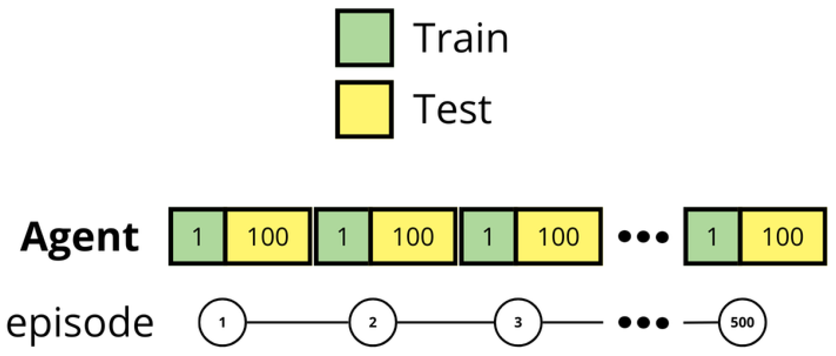
The methodology involved evaluating the agents after each training episode. During the training process, the agent was allowed to update its memory table according to the specific algorithm being employed. Following each training episode, the agent attempted to achieve the objective in the environment using the resulting memory table. This evaluation was repeated 100 times, during which the agent’s memory table remained fixed and could no longer be modified. As illustrated in Figure 1, during the training phase, the agent updates its memory table; whereas, during the testing phase, it utilizes its current memory table without making further modifications. During the test, exploration methods are disabled, including $ϵ-greedy$ in Q-Learning and the action probability in M-Learning.

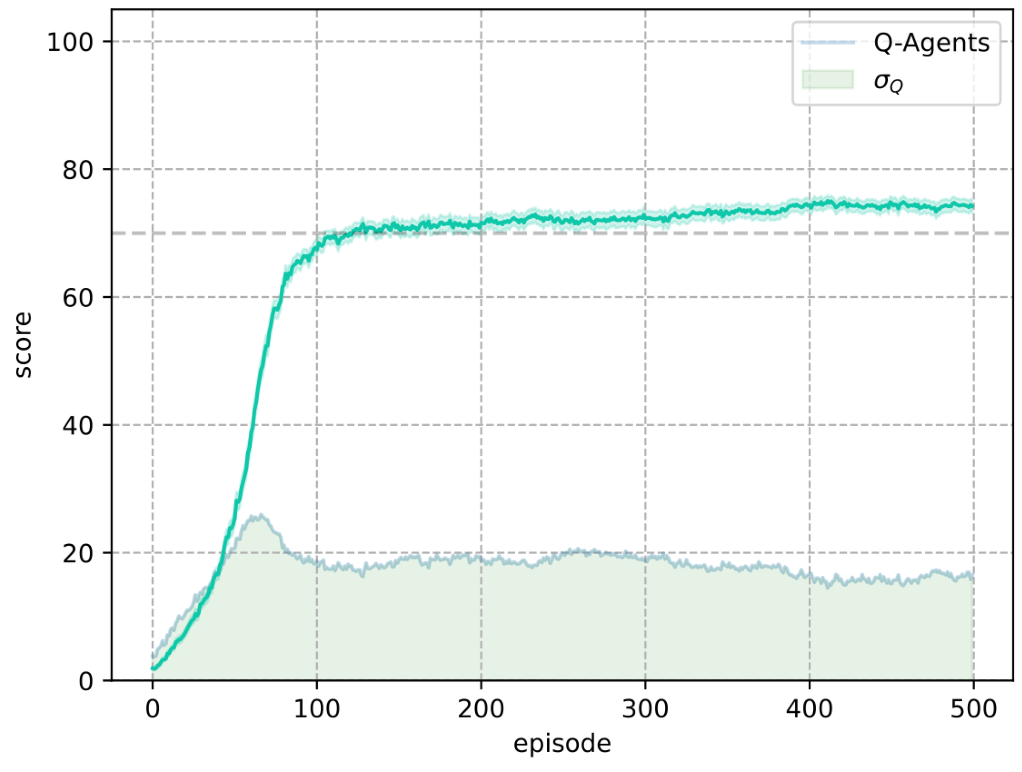
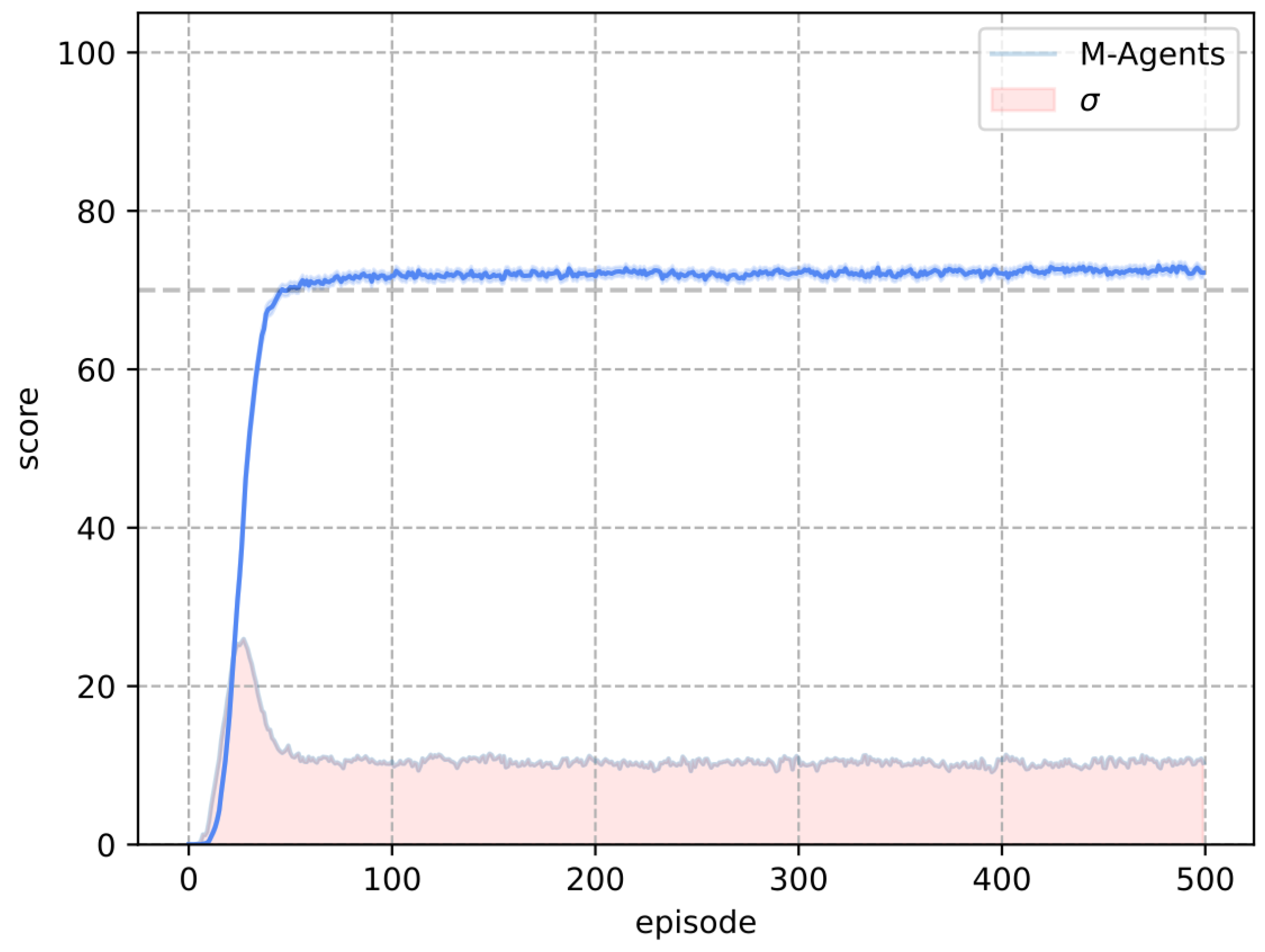
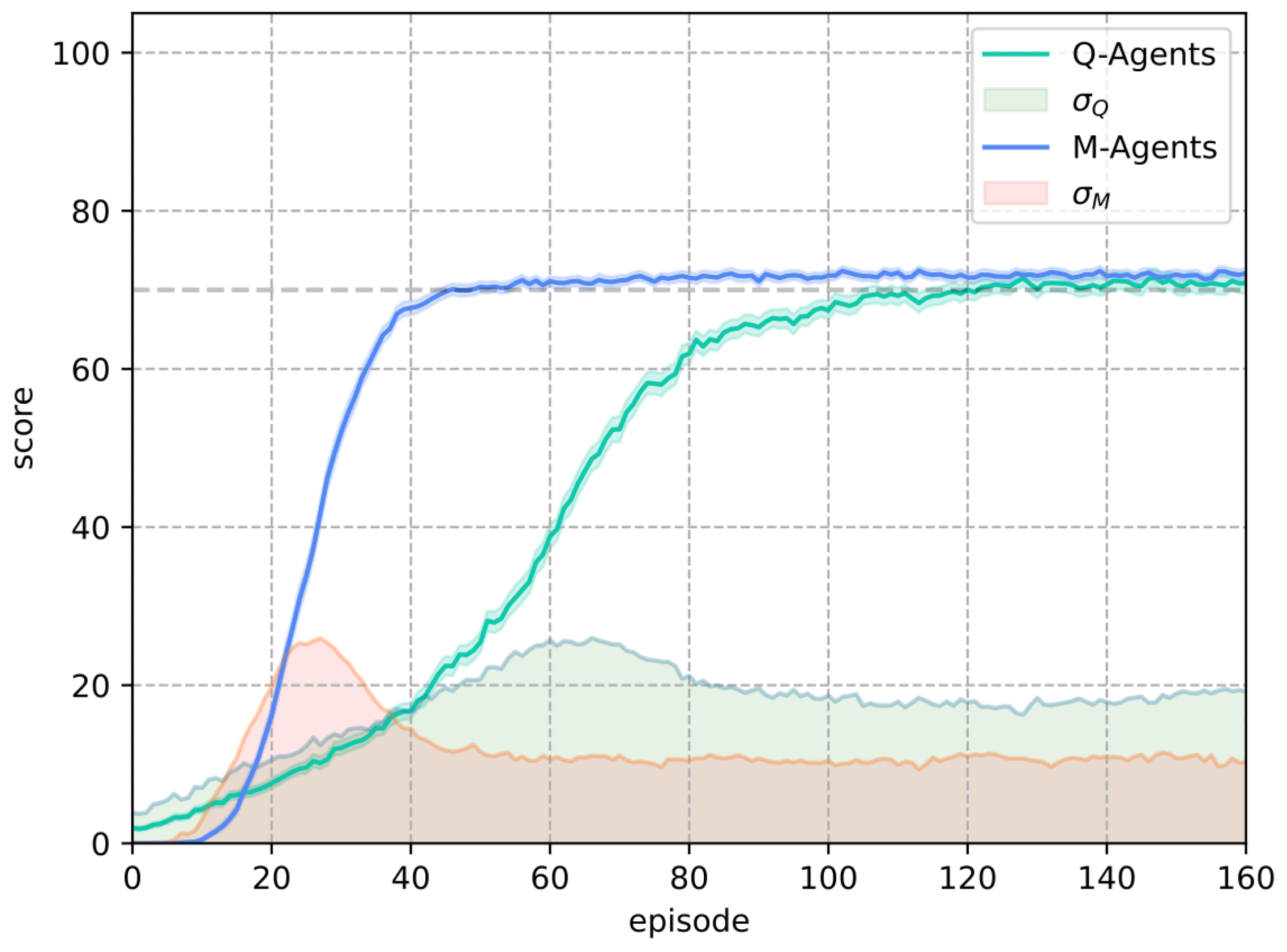
The test score used to compare both algorithms is based on the number of times the agents successfully locate the objective during testing. Evaluation is conducted over 100 attempts, measuring how often the agent achieves success following a training episode. In a deterministic environment, the outcomes are binary, resulting in either a 100% loss rate or a 100% success rate. This evaluation method is particularly valuable in stochastic environments, as it assesses the agent’s success rate under uncertain conditions.

The purpose of this test score is to evaluate how effectively the agents learn in each episode when applying the respective algorithm (Q-Learning or M-Learning). The policy implemented by both algorithms in the test involves always selecting the action with the highest value $max\left(s\right)$. This approach enables us to measure the agents’ learning progress and their ability to retain the knowledge acquired during training.

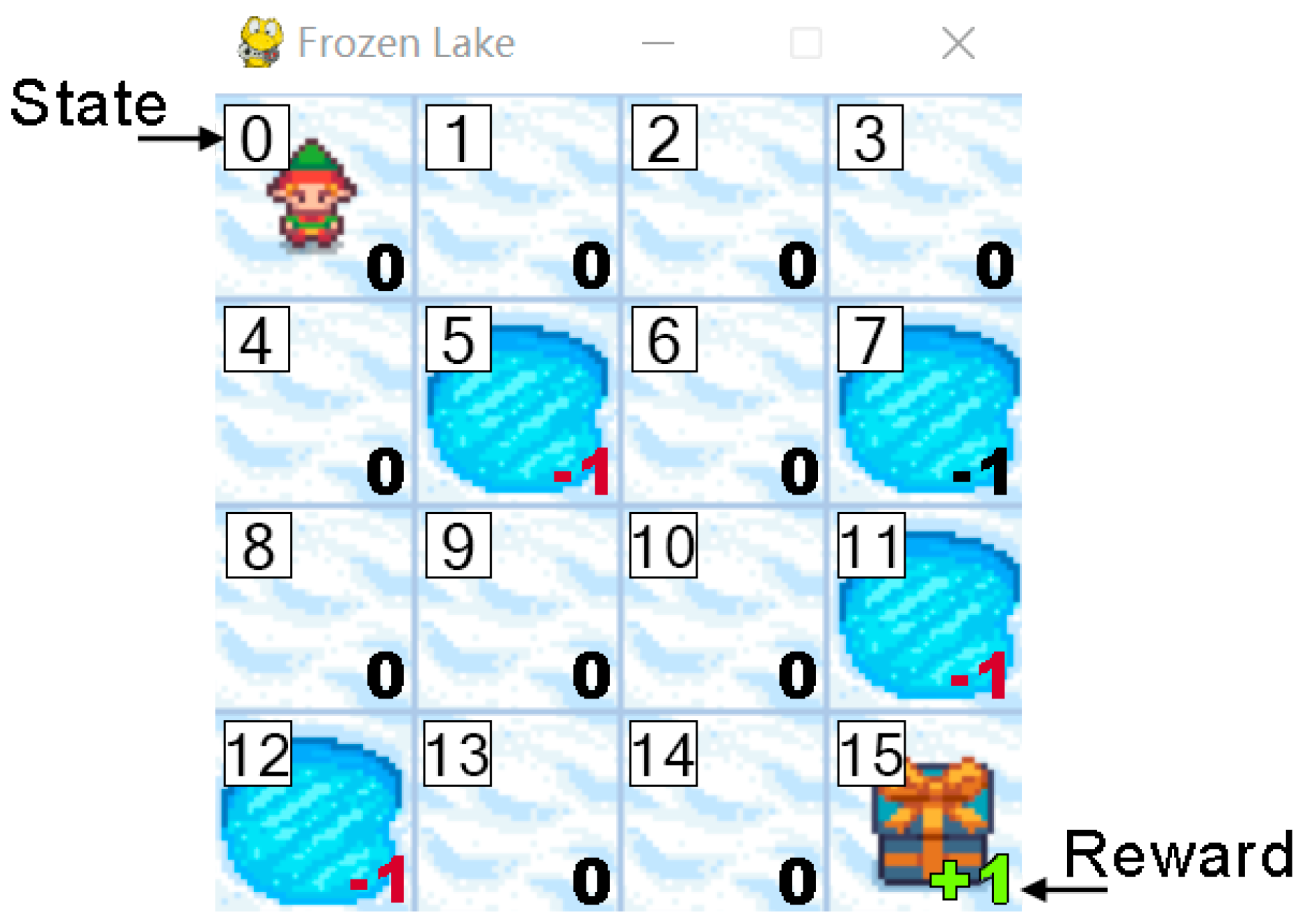
The game used for this study is Frozen Lake (Figure 2), where the objective is to cross a frozen lake without falling through a hole. The game is tested in its two modes: slippery and non-slippery, representing stochastic and deterministic environments, respectively. The tiles and, thus, the possible states of the environment are represented as integers from 0 to 15. From any position, the agent can move in four possible directions: left, down, right, or up. If the agent moves to a hole, it receives a final reward of −1, and the learning process terminates. Conversely, reaching the goal results in a reward of 1. Any other position where the agent moves results in a reward of 0.

This environment presents two variations, each representing a distinct problem for the agent. In the first variation, the environment allows the agent to move in the intended direction and the state transition function is deterministic. In the second variation, when the agent attempts to move in a certain direction, the environment may or may not guide it as intended, depending on a predefined probability. Specifically, the probability of slipping and consequently moving in an orthogonal direction to the intended one is ${\displaystyle \frac{2}{3}}$. In this case, the state transition function is stochastic.

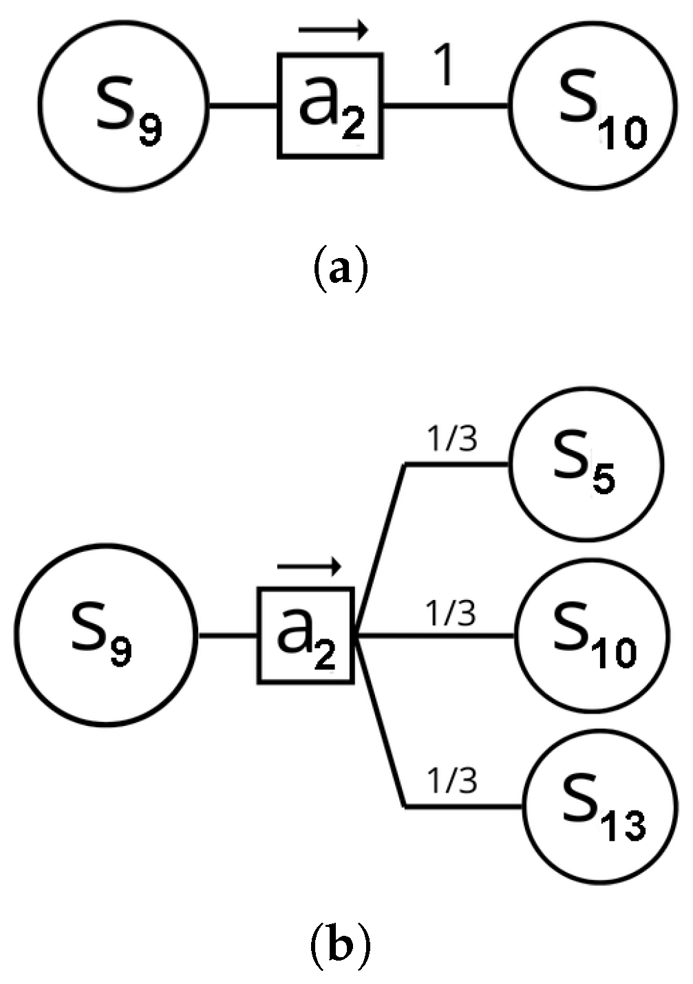
Refer to Figure 3 for a representation of the transitions. Suppose that the agent is in state $s_9$ and takes action $a_2$, moving to the right. In the deterministic environment, the probability of transitioning to state $s_{10}$ from $s_9$ upon taking action $a_2$ is 1, $P(s_{10}\mid s_9,a_2)=1$. In the stochastic environment, the probability of transitioning to state $s_{10}$ from $s_9$ upon taking action $a_2$ is $1/3$. Additionally, there are two other possible outcomes: moving to orthogonal directions, $P(s_5\mid s_9,a_2)=1/3$ and $P(s_{13}\mid s_9,a_2)=1/3$. In conclusion, in the stochastic environment, the agent has a $1/3$ probability of moving in the intended direction and a $2/3$ probability of moving in an orthogonal direction.

Frozen Lake is available in the Gymnasium library, a maintained fork of OpenAI’s Gym [24], which is described as “an API standard for reinforcement learning”. This environment is fully documented in the Gymnasium resources.

Table 2. Description of environments.

Frozen Lake Spaces
Action Space Discrete(4)	←→↑↓
Observation Space Discrete(16)	[$s_0,s_1,s_2,s_3,s_4,s_5,s_6,s_7$, $s_8,s_9,s_{10},s_{11},s_{12},s_{13},s_{14},s_{15}$]
Reward function	$r\left(s\right)=\left\{\begin{array}{ccc}1\hfill & if& s=\left\{s_{15}\right\}\hfill \\ -1\hfill & if& s=\{s_5,s_7,s_{11},s_{12}\}\hfill \\ 0\hfill & if& s=\{s_0,s_1,s_2,s_3,s_4,s_6,s_8,s_9,s_{10},s_{13},s_{14}\}\hfill \end{array}\right.$

provides a detailed description of these environments.

For the grid parameter search in Q-Learning, 200 agents were trained for each combination of algorithm parameters. After selecting the optimal parameter set for Q-Learning, an additional 1000 agents were trained to compare their results with those obtained using M-Learning.

Table 3. Configuration of experimental grid parameter search and final comparison.

Frozen Lake Experimental Configuration
	Number of Agents	Episode Limit	Step Limits
Grid parameter search	20,000	500	500
Final experiment	1000	500	500

summarizes the experimental configuration. The grid parameter search included five values for $\alpha$, five values for $\beta$, and four values for ${ϵ}_d$, resulting in a total of $5\times 5\times 4=100$ parameter combinations.

Tuning the Algorithms’ Parameters

To train agents using Q-Learning, it is crucial to appropriately configure the algorithm’s parameters. The initial values of the Q-table were initialized with pseudo-random values within the range of 0 to 1. The minimum value (${ϵ}_{min}$) for the $ϵ$-greedy policy was set to 0.005. A grid search (

Table 4. Grid parameter search for Q-Learning algorithm.

Parameter	Values
$\mathit{\alpha }$	0.1	0.3	0.5	0.7	0.9
$\gamma$	0.1	0.3	0.5	0.7	0.9
${ϵ}_d$	0.8	0.987	0.996	0.998

) was performed for $\mathit{\alpha }$, $\gamma$, and ${ϵ}_d$, as these parameters have a significant influence on the algorithm’s performance.

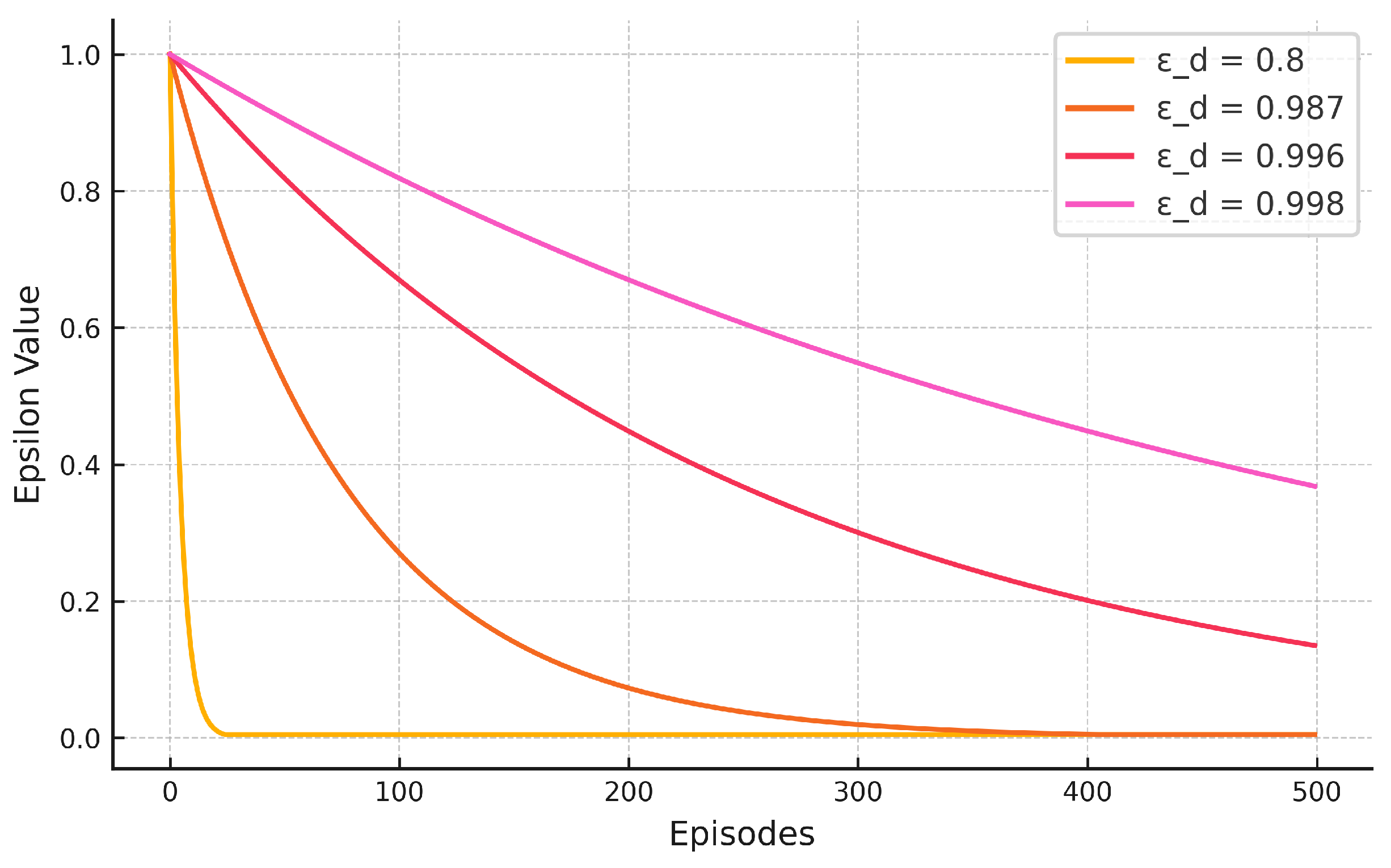
The parameters of the Q-Learning algorithm in (Table 4) are proposed to explore the space of the parameter grid search. The purpose is to see the algorithm’s behavior over the parameter space. Values of alpha and gamma are proposed to be searched uniformly since both are independent of the number of episodes. For ${ϵ}_d$, four values are proposed that maintain the exploration–exploitation balance within the range of episodes. 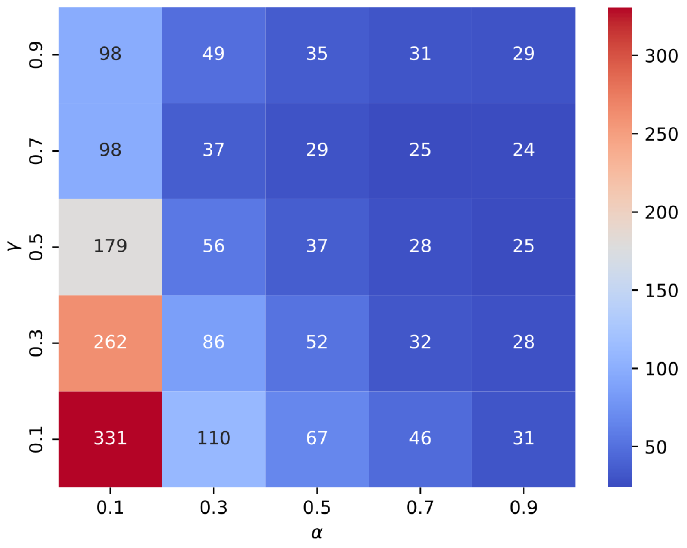Figure 4 shows the behavior of $ϵ$ with these values of ${ϵ}_d$.

The training of agents using our proposed M-Learning method involved setting the parameter $Q_{lim}$ to 0.96, as proposed by Equation (12).

4. Results

For each experiment, a dataset containing the test scores of the agents across the episodes was obtained. The score refers to the number of test episodes that the agent successfully completes. For each episode, the test scores were averaged, and a 95% confidence interval was calculated, assuming a normal distribution. In this section, the results are displayed as line graphs, with the average value plotted as a solid line in a strong color. The confidence interval is represented as a shaded area around the solid line in a fainter version of the same color.

Figure 5 and Figure 6 show the results of a grid search over parameters, using one hundred sets of parameters for Q-Learning. The vertical axis represents the number of successful tests, while the horizontal axis represents the number of episodes. Each line shows the results for a specific set of parameters, with colors corresponding to the ${ϵ}_d$ parameter. The external grid indicates the values of $\gamma$ (vertical) and $\alpha$ (horizontal) in the grid search.

To provide a measure of the dispersion of the results for the algorithms used to train the agents, the standard deviation ($\sigma$) is included in the result graphs. The value of $\sigma$ is calculated for each episode to show how it changes throughout the training process. It is defined as follows in Equation (20):

$$\sigma =\sqrt{{\displaystyle \frac{1}{N}}\sum _{i=1}^N{(x_i-\mu )}^2}$$

(20)

where

• $\sigma$ is the standard deviation of the results for a given algorithm,
• N is the total number of trained agents,
• $x_i$ represents the individual result score obtained by an agent in the episode,
• $\mu$ is the mean result score of the agents for the episode, given by

  $$\mu ={\displaystyle \frac{1}{N}}\sum _{i=1}^N{x}_i$$

For simplicity in the text labels used in the graphics, the results of agents trained with the Q-Learning algorithm are referred to as Q-Agents. Similarly, the results of agents trained with the M-Learning algorithm are referred to as M-Agents.

4.1. Deterministic Environment

This subsection presents the simulation results for the two algorithms in the deterministic environment, following the proposed experimental setup.

4.1.1. Q-Learning

The results of the grid search for the parameters of Q-Learning within the deterministic Frozen Lake environment are shown in Figure 5. In total, 20,000 agents were trained for this experiment. The results indicate that an increase in ${ϵ}_d$ causes the agents to require more episodes to find a policy. Smaller values of $\mathit{\alpha }$ increase the dispersion in the agent scores, and an increase in $\gamma$ reduces the time it takes for the agents to achieve the goal.

The proposed criterion for selecting the best set of parameters was the combination that required the fewest episodes for the mean value to achieve 100% of the test scores. The results of the deterministic environment (Figure 5) show that all the agents trained with ${ϵ}_d=0.8$ are consistently faster than with other values of ${ϵ}_d$. Based on this criterion, the results for ${ϵ}_d=0.8$, shown in

Table 5. Set of parameters requiring the lowest number of episodes to reach a score of 100 in the test.

Parameters			Test Episode 100%
$\mathit{\alpha }$	$\mathit{\gamma }$	${\mathit{ϵ}}_{\mathit{d}}$
0.1	0.1	0.8	331
0.1	0.3	0.8	262
0.1	0.5	0.8	179
0.3	0.1	0.8	110
0.1	0.7	0.8	98
0.1	0.9	0.8	98
0.3	0.3	0.8	86
0.5	0.1	0.8	67
0.3	0.5	0.8	56
0.5	0.3	0.8	52
0.3	0.9	0.8	49
0.7	0.1	0.8	46
0.3	0.7	0.8	37
0.5	0.5	0.8	37
0.5	0.9	0.8	35
0.7	0.3	0.8	32
0.7	0.9	0.8	31
0.9	0.1	0.8	31
0.5	0.7	0.8	29
0.9	0.9	0.8	29
0.7	0.5	0.8	28
0.9	0.3	0.8	28
0.7	0.7	0.8	25
0.9	0.5	0.8	25
0.9	0.7	0.8	24

, were ordered from largest to smallest.

Figure 7 shows the behavior of the exploration mesh for ${ϵ}_d=0.8$ according to the proposed criterion. Note that the best results are located in the high-value region for parameters $\mathit{\alpha }$ and $\gamma$.

The best set of parameters for $\mathit{\alpha }$, $\gamma$, and ${ϵ}_d$ was (0.9, 0.7, 0.8). All agents trained with Q-Learning obtained a score of 100 in episode 24.

Once the set of parameters had been selected, a second experiment was conducted with 1000 agents. Figure 8 shows the results obtained using the best set of parameters along with the standard deviation per episode. In this experiment, Q-Learning achieved a score of 100 in episode 26 for all agents.

4.1.2. M-Learning

Figure 9 shows the results of the M-Learning algorithm in the deterministic Frozen Lake environment. A total of 1000 agents were trained for the comparison with Q-Learning. All trained agents achieved a score of 100 in episode 18.

4.2. Stochastic Environment

This subsection presents the simulation results for the two algorithms in the stochastic environment, following the proposed experimental setup.

4.2.1. Q-Learning

The results of the grid parameter search for Q-Learning within the stochastic Frozen Lake environment are shown in Figure 6. A total of 20,000 agents were trained for this experiment. The results indicate that an increase in ${ϵ}_d$ causes the agents to require more episodes to find a policy, similarly to what occurs in the deterministic environment. The results also suggest that a larger value of $\alpha$ may lead to missing the maximum score, especially when ${ϵ}_d=0.8$ in this problem. Unlike the deterministic Frozen Lake environment, it is not possible to achieve a $100\%$ success rate in the tests, given the stochastic nature of the environment.

As a criterion for selecting a set of parameters, two conditions were proposed: (i) selecting the combination that required the fewest episodes for its mean value to exceed $70\%$ of the test scores; (ii) ensuring that, during the remaining episodes, the mean did not fall below $65\%$. The set of parameters that met the criterion is presented in

Table 6. Set of parameters requiring the lowest number of episodes to exceed a score of 70 while remaining above 65 in the rest of the test episodes.

Parameters			Test Episode 100%
$\mathit{\alpha }$	$\mathit{\gamma }$	${\mathit{ϵ}}_{\mathit{d}}$
0.3	0.3	0.998	485
0.1	0.7	0.996	459
0.1	0.3	0.998	453
0.1	0.1	0.998	446
0.1	0.5	0.996	401
0.1	0.3	0.996	358
0.5	0.9	0.987	357
0.7	0.9	0.987	351
0.1	0.1	0.996	335
0.3	0.9	0.987	315
0.1	0.7	0.987	303
0.1	0.7	0.8	259
0.1	0.5	0.987	250
0.1	0.3	0.987	239
0.3	0.7	0.987	236
0.3	0.9	0.8	194
0.1	0.5	0.8	193
0.1	0.3	0.8	156
0.5	0.9	0.8	118
0.3	0.7	0.8	101

, ordered from highest to lowest.

The best set of parameters for $\mathit{\alpha }$, $\gamma$, and ${ϵ}_d$ was (0.3, 0.7, 0.8). The agents trained with Q-Learning obtained a mean score higher than $70\%$ in episode 101.

Once the set of parameters had been selected, the second experiment was conducted with 1000 agents. Figure 10 shows the training results. In this experiment, Q-Learning met the score criteria in episode 120.

4.2.2. M-Learning

Figure 11 shows the results of the M-Learning algorithm in the stochastic Frozen Lake environment. A total of 1000 agents were trained for the comparison with Q-Learning. In this experiment, M-Learning achieved the score criteria by episode 46.

5. Discussion

5.1. Deterministic Environment

The results in the deterministic environment indicate that a policy solution is easily obtained by the algorithms. For Q-Learning, Table 5 and Figure 7 show that different sets of parameters yield the same results, demonstrating the low difficulty of the task in the environment and its limited variability. The results also highlight that longer exploration times can delay the learning of agents in environments with low difficulty.

Figure 12 presents a comparison of the solutions obtained by the agents trained with Q-Learning and M-Learning in the deterministic Frozen Lake environment. This figure shows that the M-agents achieved a score of 100 in a shorter period of time and that the standard deviation area of the score was lower than that of the Q-agents.

The standard deviation indicates that the agents trained with Q-Learning may experience losses in the acquired knowledge at some points, even if the environment remains unchanged. This behavior can be observed throughout training (see Figure 8).

Additionally, the comparison was analyzed in terms of the frequency with which the agents successfully reached the objective in each episode. For the 1000 agents, we analyze the distribution of their scores. In each episode, we determine how many agents meet the score criteria. This approach aims to reveal the overall shape and behavior of the algorithms across the general population of agents. Figure 13 presents the histogram of this comparison.

The agents trained using Q-Learning achieved the objective, on average, in episode 13.827, with a standard deviation of 4.18 episodes, whereas the agents trained using M-Learning took a mean of 12.456 episodes to meet the criteria, with a standard deviation of 1.74 episodes. This corresponds to a $9.91\%$ reduction in the mean number of episodes required to achieve the goal, as well as a $58.37\%$ reduction in the standard deviation.

5.2. Stochastic Environment

Figure 14 compares the solutions obtained by the agents trained with Q-Learning and M-Learning in the stochastic Frozen Lake environment. The comparison shows that the M-agents met the score criteria in a shorter period of time and that their standard deviation area was lower than that of the agents trained with the Q-Learning algorithm.

Figure 15 is a histogram comparing the results of Q-Learning and M-Learning in the stochastic environment. For the 1000 agents, we analyze the distribution of their scores. In each episode, we determine how many agents meet the score criteria. This approach aims to reveal the overall shape and behavior of the algorithms across the general population of agents.

The agents trained using Q-Learning met the score criteria, on average, in episode 57,591 with a standard deviation of 14.77, whereas the agents trained using M-Learning took a mean of 31,186 episodes to reach the goal, with a standard deviation of 7.42. This corresponds to a $45.84\%$ reduction in the mean number of episodes required to meet the score criteria and a $49.75\%$ reduction in the standard deviation.

6. Conclusions

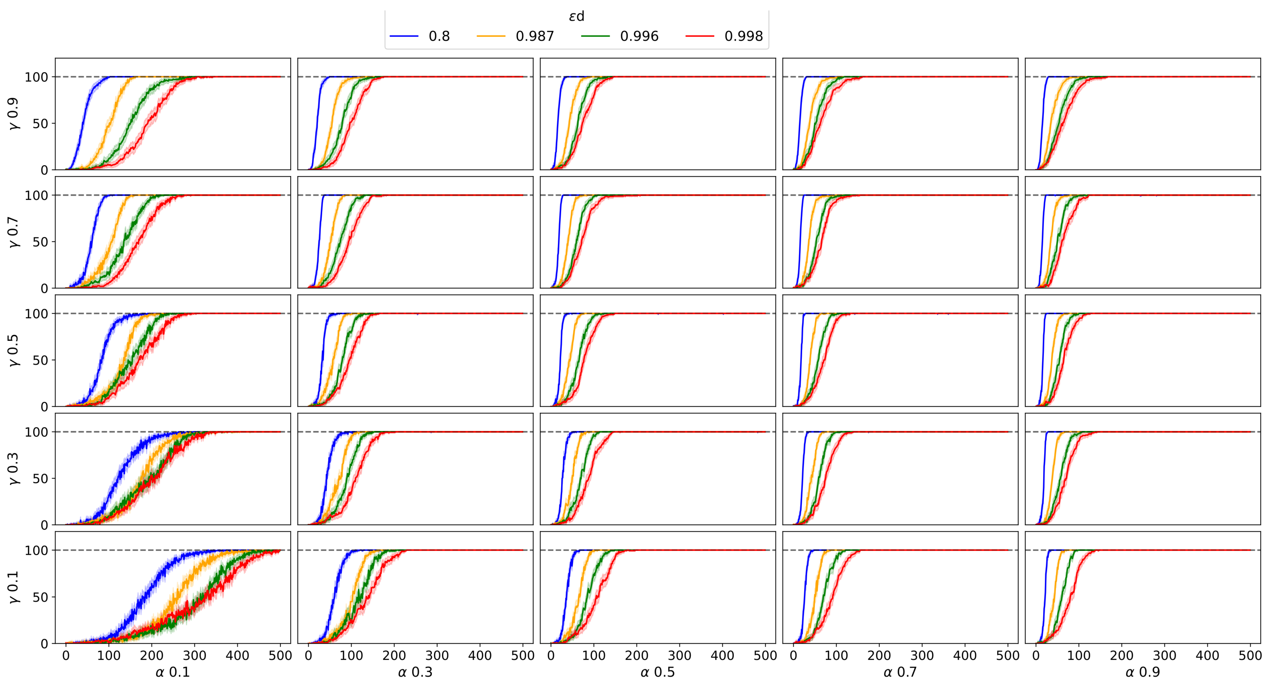
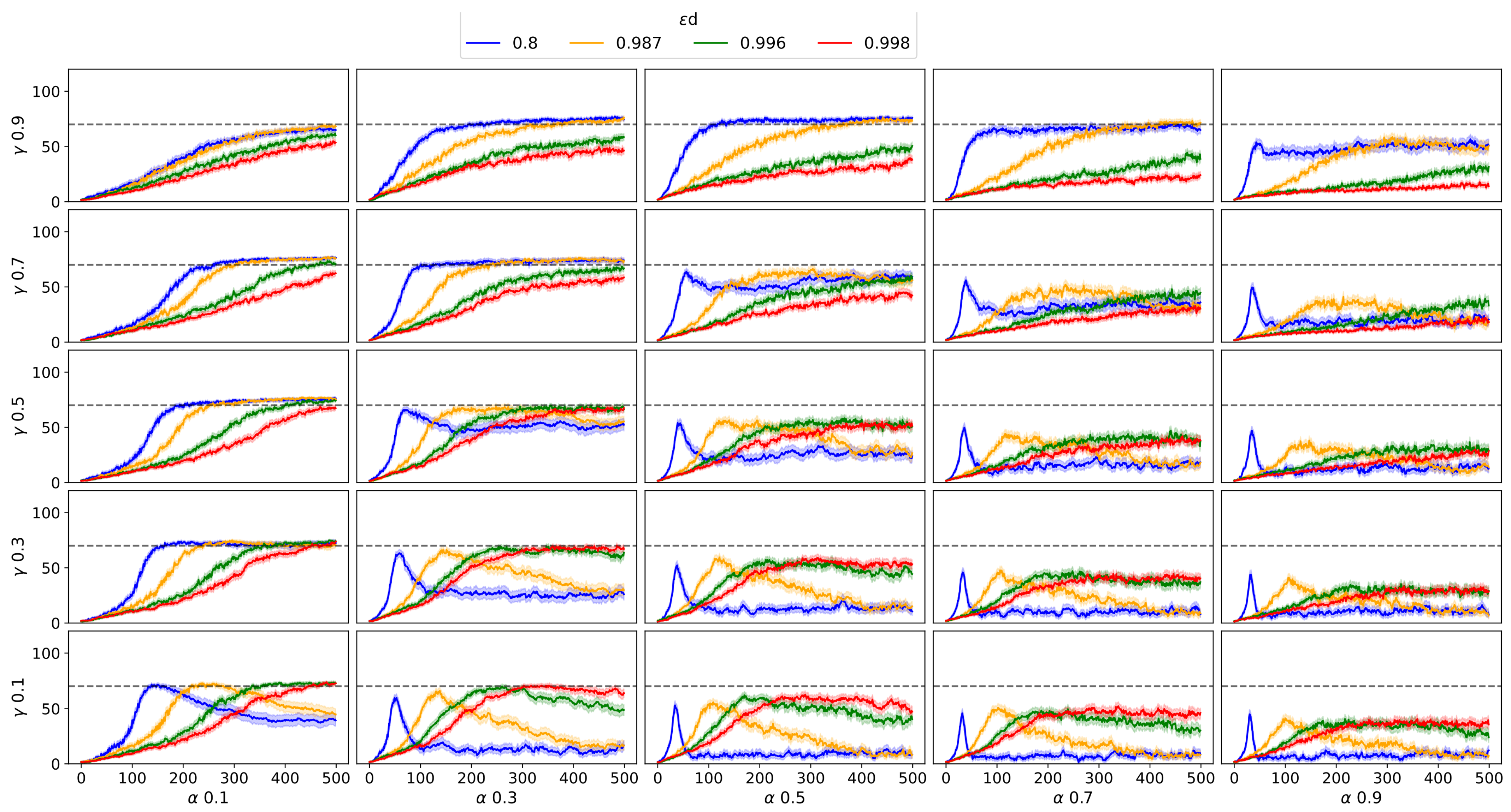
This paper presents a grid search for parameters for the deterministic and stochastic Frozen Lake environments (Figure 5 and Figure 6, respectively) when using Q-Learning. As Frozen Lake is one of the earliest and most recognized environments in RL, these experiments may be helpful for those who wish to conduct further experiments with this environment and Q-Learning.

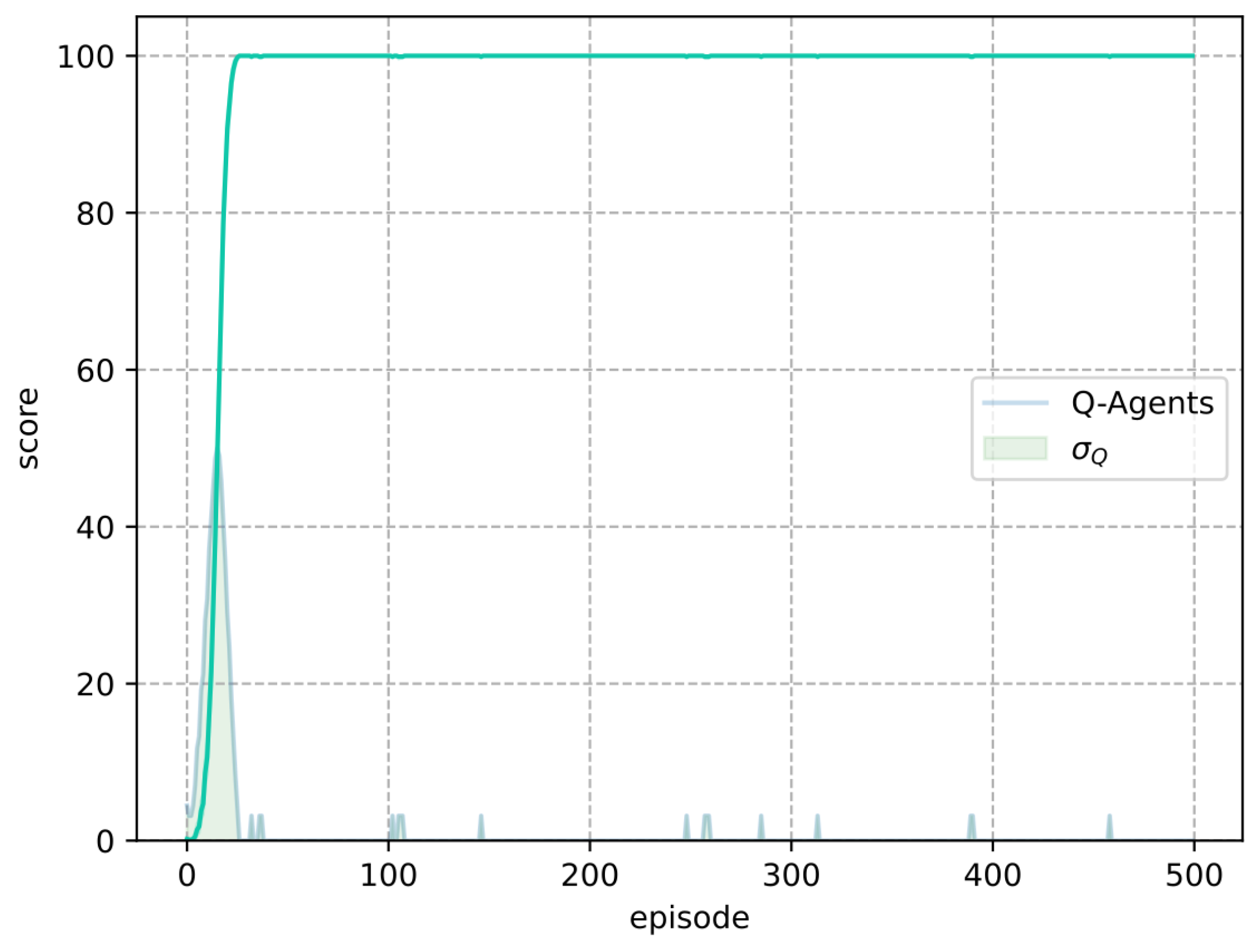
In Frozen Lake, the M-Learning algorithm trains agents faster than Q-Learning. In the deterministic environment, the number of episodes necessary for all agents to achieve a score of 100 is $30.7\%$ lower (eight episodes) for M-Learning when compared to Q-Learning. In the stochastic environment, the former requires $61.66\%$ fewer episodes (74) on average.

Additionally, in terms of the standard deviation of the score, M-Learning demonstrates greater consistency in the training results. Compared to the standard deviation of Q-Learning, M-Learning shows a reduction of $58.37\%$ in the deterministic environment, as well as a reduction of $49.75\%$ in the stochastic environment.

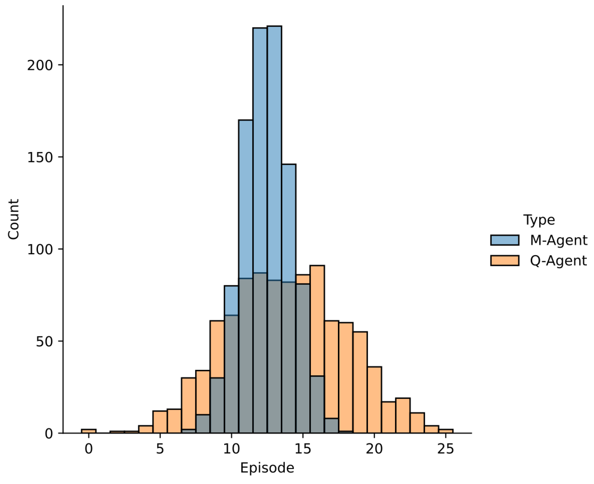
Furthermore, in both deterministic and stochastic environments, the difference in M-Learning’s result distributions (Figure 13 and Figure 15) compared to Q-Learning becomes more pronounced as complexity increases. This highlights M-Learning’s consistency despite growing environmental complexity, without requiring parameter adjustments. Notably, M-Learning maintained the same parameter $Q_{lim}$, while Q-Learning required a grid search to optimize its parameters, which varied across environments.

Finally, the main contribution of this paper consists of two interconnected aspects, both of which stem from the formulation of the proposed M-Learning algorithm.

• The most relevant aspect is that the exploration–exploitation dilemma can be self-regulated based on the value of actions in the states, which eliminates the need to use the additional parameters demanded by the $ϵ$-greedy policy.
• The second one is that considering the value of actions with a probabilistic approach allows modifying the value of all actions in a state through a single interaction with the environment.

While the above can be understood from different perspectives, it is ultimately the result of a unified approach.

Future Work

With the results obtained for M-Learning, we suggest that future research should focus on evaluating its performance in other environments with the purpose of identifying the specific problems where it may prove most useful.

The factor $\mathbf{m}$, which modifies the value of an action, offers a promising avenue for further exploration. Future studies could investigate alternative methods for calculating this factor, either to simplify the process or to incorporate additional sources of information beyond the reward and the knowledge stored in the states.