Ring-like Bright Monster Waves in Variable-Coefficient Partially Nonlocal Coupled NLS Equations with Directional Diffraction and External Perturbations in (3+1)D

Abstract

Partially nonlocal (PNL) variable-coefficient nonlinear Schrödinger equations (NLSEs) represent a significant area of study in mathematical physics and quantum mechanics, particularly in scenarios where potential and coefficients vary spatially or temporally. The (3+1)-dimensional partially nonlocal (PNL) coupled nonlinear Schrödinger (NLS) model, enriched with different values of two transverse diffraction profiles and subjected to gain or loss phenomena, undergoes dimensional reduction to a (2+1)-dimensional counterpart model, facilitated by a conversion relation. This reduction unveils intriguing insights into the excited mechanisms underlying partially nonlocal waves, culminating in analytical solutions that describe high-dimensional extreme waves characterized by Hermite–Gaussian envelopes. This paper explores novel extreme wave solutions in (3+1)-dimensional PNL systems, employing Hirota’s bilinearization method to derive analytical solutions for ring-like bright–bright vector two-component one-soliton solutions. This study examines the dynamic evolution of these solutions under varying dispersion and nonlinearity conditions and investigates the impact of gain and loss on their behavior. Furthermore, the shape of the obtained solitons is determined by the parameters s and q, while the Hermite parameters p and n modulate the formation of additional layers along the z-axis, represented by $p+1$ and $n+1$, respectively. Our findings address existing gaps in understanding extreme waves in partially nonlocal media and offer insights into managing these phenomena in practical systems, such as optical fibers. The results contribute to the theoretical framework of high-dimensional wave phenomena and provide a foundation for future research in wave dynamics and energy management in complex media.

1. Introduction

Partially nonlocal (PNL) variable-coefficient nonlinear Schrödinger equations (NLSEs) are a specialized area of study within mathematical physics and theoretical quantum mechanics. They typically arise in contexts where the potential and coefficients in the NLSE vary with respect to space, time, or both. The “partially nonlocal” aspect implies that the equation involves nonlocal terms that depend on the spatial variables, but these nonlocal terms may not extend over the entire spatial domain. Variable coefficients mean that the coefficients of the equation, such as the potential term, can vary spatially and/or temporally. Over the last several years, various researchers have intensified investigations into localized excitations in media where PNL effects are involved. A pivotal contribution in this field was made by Mitchell and Snyder in 1999, who introduced an analytical method for analyzing beam dynamics in PNL media [1].

This foundational work paved the way for subsequent research, including the development of solutions for (2+1)-dimensional and (3+1)-dimensional variable coefficient NLSEs without the influence of external potentials [2,3], and with the influence of external potentials [4,5,6,7,8,9,10,11,12,13,14,15]. The potentials added to the distributed-coefficient PNL-NLSEs are linear [4,5,6,7], harmonic, or parabolic [8,9,10], and linear and harmonic [11,12]. Based on these models, researchers have identified various localized structures, such as spatiotemporal Hermite–Gaussian vortex soliton solutions [2], spatiotemporal Hermite–Gaussian solitons [3], vector and scalar crossed double-Ma breathers [4], matter-wave solutions [5], torus-shaped vortex solitons, ring-vortex solitons [6], ring-like Kuznetsov–Ma and Akhmediev breathers [7], Peregrine solutions and combined Akhmediev breathers [8], vortex solitons, dipole solitons, saddle-shaped solitons [9], ring-like two-breather solutions [10], ring-like partially nonlocal extreme waves [11], ring-like double-breather solutions [12], scalar and vector rogue waves [13], Peregrine solutions with breather excitation [14], and rogue waves [15].

Recent progress in the field has led to the development of coupled PNL-NLS models for analyzing two-component wave dynamics in both optical systems and Bose–Einstein condensates [4,16,17,18,19,20,21,22,23,24,25,26,27,28]. Notably, research has documented (2+1)-dimensional nonlocal vector solitons and breathers in nonautonomous PNL media influenced by external potentials [4,16]. Investigations have also focused on managing (3+1)-dimensional nonlocal scalar and vector solitons [17,18,20], including studies of nonlocal vector bright–dark one- and two-soliton phenomena [19]. Additionally, significant research has been devoted to two-component rogue waves [21], and the discovery and characterization of bright–dark and bright–bright monster waves [22]. Specific wave types, such as bright–dark second-order rogue waves and triplets [23], bright–bright Peregrine quartets [24], and bright–dark Peregrine three sisters [25], have been thoroughly explored. High-dimensional vector soliton solutions have also been prominently featured [26]. The theoretical framework has been extended with solutions for bright–dark vector two-component one-soliton and two-soliton systems, as well as vector two-component first-order localized solitons [27]. Furthermore, ring-like bright–dark monster wave solutions have been extensively investigated [28]. These studies have collectively enhanced our understanding of complex wave phenomena across various physical contexts. The interest in (3+1)-dimensional structures arises from their enhanced ability to accurately model the evolution of real matter or optical waves, providing a more faithful representation than lower-dimensional soliton models. This improved accuracy is essential for gaining insights into practical scenarios and guiding numerical simulations that address real-world challenges [10]. However, a significant gap remains in understanding extreme wave solutions in partially nonlocal media. Despite some efforts to begin addressing this issue, particularly by Yomba in the context of partially nonlocal (PNL) media [29,30], the study of extreme waves—characterized by varying diffraction properties and influenced by external potentials, as well as gain or loss effects—remains relatively unexplored. The inclusion of gain and loss terms in other contexts is particularly relevant due to their impact on real systems, such as optical fibers, where energy loss during transmission is a common issue [31,32]. Previous studies have highlighted the importance of addressing gain or loss phenomena, especially in optical soliton transmission. This has led to the development of compensation strategies, including optical gain via Raman amplification [33] and advanced techniques for managing dispersion and nonlinearity [20,34,35].

This paper seeks to continue addressing existing gaps by investigating the potential existence of novel extreme waves localized in (3+1)-dimensional space. We will accomplish this by analyzing a (3+1)-dimensional partially nonlocal coupled NLS system, which is influenced by linear and harmonic potentials, as well as gain or loss effects. This system can be simplified to a (2+1)-dimensional autonomous equation. Using Hirota’s bilinearization method to solve the constant-coefficient coupled equations, we will search for approximate solutions representing ring-like bright–bright vector two-component one-soliton solutions. Additionally, we will explore the dynamic evolution of these waves under various dispersion and nonlinearity management conditions and examine how gain or loss terms affect their behavior. This study introduces a novel approach to vector self-similar soliton dynamics in inhomogeneous optical media, offering a distinct perspective from previous works [29,30]. In [29], self-similar reduction and ansatz techniques were employed to derive first- and second-order ring-like extreme waves, whereas [30] utilized self-similar reduction and other ansatz techniques to obtain Akhmediev (AB), Ma (MB), and Akhmediev–Ma (AMB) breather solutions. This work advances beyond these approaches by introducing ring-like bright–bright vector two-component solitons, which exhibit both spatial and temporal localization, distinguishing them from the static solutions found in [29,30]. Unlike these previous works, the solitons presented here evolve dynamically, capturing their interactions, formation, and transformations in inhomogeneous media. A key advancement of this study is the application of Hirota’s method, which enables the construction of multi-soliton solutions, allowing for a deeper exploration of soliton interactions over time. Unlike the self-similar reduction and ansatz techniques used in prior studies, Hirota’s method offers a systematic framework for deriving exact soliton solutions, making it particularly effective in analyzing vector solitons and their evolution in nonlinear optical systems. This study stands out for its dynamic soliton solutions and the systematic application of Hirota’s method, providing a broader and more insightful analysis of nonlinear wave behavior than the extreme wave and breather solutions in [29,30].

The structure of this paper is organized as follows. Section 2 establishes a transformation that links the (3+1)-dimensional variable-coefficient PNL coupled NLS model with a (2+1)-dimensional constant-coefficient coupled model and presents analytical solutions for ring-like extreme waves. Section 3 offers an in-depth analysis of the characteristics and evolution of these extreme waves. Finally, Section 4 summarizes the key findings of this study.

2. Converting Formula and Extreme Wave Solutions

We explore the factors that affect the formation of higher-dimensional extreme waves localized in a (3+1)-dimensional space. This study focuses on the nonautonomous (3+1)-dimensional partially nonlocal (PNL) coupled nonlinear Schrödinger (NLS) system. The system demonstrates unique diffraction properties in different spatial directions, constrained by linear and parabolic potentials, and is influenced by external factors such as gain or loss [29,30].

$$i{\displaystyle \frac{\partial }{\partial t}}{q}_1+{\beta }_1(t){\displaystyle \frac{{\partial }^2{q}_1}{\partial x^2}}+{\beta }_2(t){\displaystyle \frac{{\partial }^2{q}_1}{\partial y^2}}+\kappa (t)q_1{\int }_{-\infty }^{\infty }({ϵ}_{11}|q_1{|}^2+{ϵ}_{12}|q_2{|}^2)dz+$$

$$({\tau }_1(t)x+{\tau }_2(t)y+{\chi }_1(t)x^2+{\chi }_2(t)y^2)q_1+i{\mathsf{\Gamma }}_1(t)q_1=0,$$

$$i{\displaystyle \frac{\partial }{\partial t}}{q}_2+{\beta }_1(t){\displaystyle \frac{{\partial }^2{q}_2}{\partial x^2}}+{\beta }_2(t){\displaystyle \frac{{\partial }^2{q}_2}{\partial y^2}}+\kappa (t)q_2{\int }_{-\infty }^{\infty }({ϵ}_{21}|q_1{|}^2+{ϵ}_{22}|q_2{|}^2)dz+$$

$$({\tau }_1(t)x+{\tau }_2(t)y+{\chi }_1(t)x^2+{\chi }_2(t)y^2)q_2+i{\mathsf{\Gamma }}_2(t)q_2=0,$$

(1)

which is a generalization of the (3+1)-dimensional coupled PNL-NLS model in [25,26,27,28]. The quantities t and $x,y,z$ serve as independent variables scaling the temporal and three spatial components, respectively. The complex field quantities $q_j(t,x,y,z)$ with $j=1,2$ represent two vector components of normalized light-field envelopes in optics or mean-field wave vector functions in Bose–Einstein condensates (BECs). The coefficients ${\beta }_j,{\tau }_j,$ and ${\chi }_j$ correspond to diffractions, linear potentials, and parabolic potentials, respectively. $\kappa$ denotes the coefficient of PNL nonlinearity, exhibiting locality in the x- and y-directions and nonlocality in the z-direction [22]. Additionally, ${\mathsf{\Gamma }}_j$ represents the coefficient of gain (${\mathsf{\Gamma }}_j>0$) or loss (${\mathsf{\Gamma }}_j<0$). All parameters ${\beta }_j,{\tau }_j,{\chi }_j,\kappa$, and $\mathsf{\Gamma }$ are real functions of t. The parameters ${ϵ}_{1j}$ and ${ϵ}_{2j}$ determine the coupling strengths of cross-phase modulation and self-phase modulation, respectively. If ${\mathsf{\Gamma }}_j(t)=0$ and ${\chi }_j(t)=0$, Equation (1) corresponds to the model in [28], governing vector matter waves with intra- and interspecies atomic nonlocal interactions in BECs [24,25]. If ${\mathsf{\Gamma }}_j(t)=0,{\tau }_j(t)=0$ and ${\chi }_2={\chi }_1$ (1) becomes the model in [26], which is the (3+1)-dimensional generalization of the (2+1)-dimensional coupled Gross–Pitaevskii equation in [13].

Following the process described in [29,30], we can convert the variable-coefficient (1) into the constant-coefficient coupled equations

$$i{\mathsf{\Psi }}_{1\sigma }+K({\mathsf{\Psi }}_{1\eta \eta }+{\mathsf{\Psi }}_{1\xi \xi })+({ϵ}_{11}|{\mathsf{\Psi }}_1{|}^2+{ϵ}_{12}|{\mathsf{\Psi }}_2{|}^2){\mathsf{\Psi }}_1=0,$$

$$i{\mathsf{\Psi }}_{2\sigma }+K({\mathsf{\Psi }}_{2\eta \eta }+{\mathsf{\Psi }}_{2\xi \xi })+({ϵ}_{21}|{\mathsf{\Psi }}_1{|}^2+{ϵ}_{22}|{\mathsf{\Psi }}_2{|}^2){\mathsf{\Psi }}_2=0,$$

(2)

through the lens transformation

$$q_1(t,x,y,z)={\psi }_1(t,z){\mathsf{\Psi }}_1(\eta (t,x),\xi (t,y),\sigma (t))exp(i{\rho }_1(t,x,y,z)),$$

$$q_2(t,x,y,z)={\psi }_2(t,z){\mathsf{\Psi }}_2(\eta (t,x),\xi (t,y),\sigma (t))exp(i{\rho }_2(t,x,y,z)),$$

(3)

where the connected variables, including the accumulated time $\sigma (t)$, two mapping variables $\eta (t,x)$ and $\xi (t,y)$, the amplitude ${\psi }_j(t,z)$, and the phase ${\rho }_j(t,x,y,z)$, meet [29,30]:

$${\psi }_{1t}+{\psi }_1({\beta }_1{\rho }_{1xx}+{\beta }_2{\rho }_{1yy})+{\mathsf{\Gamma }}_1{\psi }_1=0,{\psi }_{2t}+{\psi }_2({\beta }_1{\rho }_{2xx}+{\beta }_2{\rho }_{2yy})+{\mathsf{\Gamma }}_2{\psi }_2=0,$$

(4)

$${\eta }_t+2{\beta }_1{\eta }_x{\rho }_{1x}=0,{\xi }_t+2{\beta }_2{\xi }_y{\rho }_{1y}=0,$$

$${\eta }_t+2{\beta }_1{\eta }_x{\rho }_{2x}=0,{\xi }_t+2{\beta }_2{\xi }_y{\rho }_{2y}=0,$$

(5)

$${\rho }_{1t}+({\beta }_1{\rho }_{1x}^2+{\beta }_2{\rho }_{1y}^2)-({\tau }_{1}x+{\tau }_{2}y)-({\chi }_1{x}^2+{\chi }_2{y}^2)=0,$$

$${\rho }_{2t}+({\beta }_1{\rho }_{2x}^2+{\beta }_2{\rho }_{2y}^2)-({\tau }_{1}x+{\tau }_{2}y)-({\chi }_1{x}^2+{\chi }_2{y}^2)=0,$$

(6)

$${\eta }_{xx}=0,{\xi }_{yy}=0,$$

(7)

$${\displaystyle \frac{{\beta }_1}{{\sigma }_t}}{\eta }_x^2=K,{\displaystyle \frac{{\beta }_2}{{\sigma }_t}}{\xi }_y^2=K,{\displaystyle \frac{\kappa }{{\sigma }_t}}{\int }_{-\infty }^{\infty }{\psi }_1^{2}dz=1,{\displaystyle \frac{\kappa }{{\sigma }_t}}{\int }_{-\infty }^{\infty }{\psi }_2^{2}dz=1,$$

(8)

where the subscripts imply partial differentiation. The aforementioned set of Equations (4)–(8) can be solved self-consistently to obtain the self-similar wave amplitude ${\psi }_j(t,z)$:

$${\psi }_1(t,z)={\displaystyle \frac{\sqrt{g}}{\sqrt[4]{\pi }\sqrt{2^{p}p!}}}exp\left({\int }_0^t\left(4a_1(\zeta ){\beta }_1(\zeta )-\mathsf{\Gamma }(\zeta )\right)d\zeta -{\displaystyle \frac{g^2{z}^2}{2}}\right)H_p(gz),$$

$${\psi }_2(t,z)={\displaystyle \frac{\sqrt{g}}{\sqrt[4]{\pi }\sqrt{2^{n}n!}}}exp\left({\int }_0^t\left(4a_1(\zeta ){\beta }_1(\zeta )-\mathsf{\Gamma }(\zeta )\right)d\zeta -{\displaystyle \frac{g^2{z}^2}{2}}\right)H_n(gz),$$

(9)

the phase ${\rho }_j(t,x,y,z)$ as given in [29,30]:

$${\rho }_1(t,x,y,z)=-\left(a_1(t)\left(x^2+{\displaystyle \frac{l_0^2}{k_0^2}}{y}^2\right)+b_1(t)x+b_2(t)y+{\displaystyle \frac{1}{l_0^2}}{\int }_0^t(l_0^2{b}_1{(\zeta )}^2+k_0^2{b}_2{(\zeta )}^2){\beta }_1(\zeta )d\zeta \right)+h_1(z),$$

$${\rho }_2(t,x,y,z)=-\left(a_1(t)\left(x^2+{\displaystyle \frac{l_0^2}{k_0^2}}{y}^2\right)+b_1(t)x+b_2(t)y+{\displaystyle \frac{1}{l_0^2}}{\int }_0^t(l_0^2{b}_1{(\zeta )}^2+k_0^2{b}_2{(\zeta )}^2){\beta }_1(\zeta )d\zeta \right)+h_2(z),$$

(10)

the accumulated time as given in [29,30]:

$$\sigma (t)={\displaystyle \frac{k_0^2}{K}}\left({\int }_0^t{\beta }_1(\varsigma )e^{8{\int }_0^{\varsigma }{a}_1(\zeta ){\beta }_1(\zeta )d\zeta }d\varsigma \right),$$

(11)

and two formal transformation functions as given in [29,30]:

$$\eta (t,x)=k_0\left(2{\int }_0^t{b}_1(\varsigma ){\beta }_1(\varsigma )e^{4{\int }_0^{\varsigma }{a}_1(\zeta ){\beta }_1(\zeta )d\zeta }d\varsigma +x{e}^{{\int }_0^{t}4a_1(\zeta ){\beta }_1(\zeta )d\zeta }\right),$$

(12)

$$\xi (t,y)=l_0\left(2{\displaystyle \frac{k_0^2}{l_0^2}}{\int }_0^t{b}_2(\varsigma ){\beta }_1(\varsigma )e^{4{\int }_0^{\varsigma }{a}_1(\zeta ){\beta }_1(\zeta )d\zeta }d\varsigma +y{e}^{{\int }_0^{t}4a_1(\zeta ){\beta }_1(\zeta )d\zeta }\right).$$

(13)

where the functions of the parabolic phase $a_1$ and the linear phases $b_1$ and $b_2$ satisfy the following differential equations [29,30]:

$$a_1^{\prime }(t)-4a_1{(t)}^2{\beta }_1(t)-{\chi }_1(t)=0,b_1^{\prime }(t)-4a_1(t)b_1(t){\beta }_1(t)+{\tau }_1(t)=0,b_2^{\prime }(t)-4a_1(t)b_2(t){\beta }_1(t)+{\tau }_2(t)=0.$$

(14)

Furthermore, the following constraints on the management parameters describing the linear, parabolic, diffraction, and partial nonlocality of nonlinearity can be derived [29,30]:

$${\displaystyle \frac{l_0^2}{k_0^2}}(a_1^{\prime }(t)-4a_1{(t)}^2{\beta }_1(t))+{\chi }_2(t)=0,{\mathsf{\Gamma }}_2(t)={\mathsf{\Gamma }}_1(t)=\mathsf{\Gamma }(t).$$

$${\beta }_2(t)={\displaystyle \frac{k_0^2}{l_0^2}}{\beta }_1(t),\kappa (t)={\displaystyle \frac{k_0^2}{K}}{\beta }_1(t)e^{{\int }_0^t{e}^{2\mathsf{\Gamma }(\zeta )}d\zeta }.$$

(15)

These conditions indicate that, for exact self-similar solutions of the PNL-NLS system (1), only five of its nine parameters ${\beta }_1,{\chi }_1,{\tau }_1,{\tau }_2,$ and ${\mathsf{\Gamma }}_1$ are free parameters. For instance, if ${\beta }_1,{\chi }_1,{\tau }_1,{\tau }_2$, and ${\mathsf{\Gamma }}_1$ are selected to be free parameters, then ${\beta }_2,{\chi }_2,\kappa$, and ${\mathsf{\Gamma }}_2$ are determined from (15). Here, $h_j(z)$ represents arbitrary functions, while $H_p(gz)$ and $H_n(gz)$ represent Hermite polynomials with the exponent parameter g and the non-negative integer Hermite parameters p and n, respectively. Additionally, $k_0$ and $l_0$ are associated with the wave’s width in the x- and y-directions as well as its phase. The general wave solution outlined in (3) plays a crucial role in constructing various localized waves within a realistic system governed by the variable coefficient PNL-NLS system (1). Analyzing expressions (9)–(15) reveals that the characteristics of the self-similar waves, including the amplitude, phase, and accumulated time, are affected by the diffraction in the x-direction, represented by ${\beta }_1$. Therefore, the transformation from the variable-coefficient coupled Equation (1) to the constant-coefficient coupled Equation (2) is given by [29,30]

$$\begin{array}{c}{q}_1(t,x,y,z)={\displaystyle \frac{\sqrt{g}}{\sqrt[4]{\pi }\sqrt{2^{p}p!}}}exp\left({\int }_0^t\left(4a_1(\zeta ){\beta }_1(\zeta )-\mathsf{\Gamma }(\zeta )\right)d\zeta -{\displaystyle \frac{g^2{z}^2}{2}}\right)H_p(gz)\times \\ {\mathsf{\Psi }}_1(\eta (t,x),\xi (t,y),\sigma (t))exp(i{\rho }_1(x,y,z,t)),\end{array}$$

(16)

$$\begin{array}{c}{q}_2(t,x,y,z)={\displaystyle \frac{\sqrt{g}}{\sqrt[4]{\pi }\sqrt{2^{n}n!}}}exp\left({\int }_0^t\left(4a_1(\zeta ){\beta }_1(\zeta )-\mathsf{\Gamma }(\zeta )\right)d\zeta -{\displaystyle \frac{g^2{z}^2}{2}}\right)H_n(gz)\times \\ {\mathsf{\Psi }}_2(\eta (t,x),\xi (t,y),\sigma (t))exp(i{\rho }_2(x,y,z,t)),\end{array}$$

(17)

given the two corresponding variables $\eta (t,x)$ and $\xi (t,y)$ in Equations (12) and (13), the accumulated time $\sigma (t)$ in Equation (11), and the phases ${\rho }_1(x,y,z,t)$ and ${\rho }_2(x,y,z,t)$ in Equation (10), the six constraints (14) and (15) must be satisfied as integrability conditions for Equation (1).

Using the solutions of Equation (2) and applying the corresponding relations (16) and (17), one can derive the solutions for Equation (1).

Next, rewriting Equation (2) in polar coordinates leads to [29,30]

$$i{\displaystyle \frac{\partial {\mathsf{\Psi }}_1}{\partial \sigma }}+K\left({\displaystyle \frac{{\partial }^2{\mathsf{\Psi }}_1}{\partial r^2}}+{\displaystyle \frac{1}{r}}{\displaystyle \frac{\partial {\mathsf{\Psi }}_1}{\partial r}}+{\displaystyle \frac{1}{r^2}}{\displaystyle \frac{{\partial }^2{\mathsf{\Psi }}_1}{\partial {\theta }^2}}\right)+({ϵ}_{11}|{\mathsf{\Psi }}_1{|}^2+{ϵ}_{12}|{\mathsf{\Psi }}_2{|}^2){\mathsf{\Psi }}_1=0,$$

$$i{\displaystyle \frac{\partial {\mathsf{\Psi }}_2}{\partial \sigma }}+K\left({\displaystyle \frac{{\partial }^2{\mathsf{\Psi }}_2}{\partial r^2}}+{\displaystyle \frac{1}{r}}{\displaystyle \frac{\partial {\mathsf{\Psi }}_2}{\partial r}}+{\displaystyle \frac{1}{r^2}}{\displaystyle \frac{{\partial }^2{\mathsf{\Psi }}_2}{\partial {\theta }^2}}\right)+({ϵ}_{21}|{\mathsf{\Psi }}_1{|}^2+{ϵ}_{22}|{\mathsf{\Psi }}_2{|}^2){\mathsf{\Psi }}_2=0,$$

(18)

with the radius $r=\sqrt{{\eta }^2+{\xi }^2}$ and the azimuthal angle $\theta =arctan(\xi /\eta ).$

We consider the optical fields of the form

$${\mathsf{\Psi }}_1(r,\theta ,\sigma )=A_1(r,\sigma ){\mathsf{\Theta }}_1(\theta ),{\mathsf{\Psi }}_2(r,\theta ,\sigma )=A_2(r,\sigma ){\mathsf{\Theta }}_2(\theta ).$$

(19)

By inserting Equation (19) into Equation (18), the separation of variables yields the following two equations:

$$-{\displaystyle \frac{1}{{\mathsf{\Theta }}_1}}{\displaystyle \frac{{\partial }^2{\mathsf{\Theta }}_1}{{\partial }^2\theta }}=m^2,-{\displaystyle \frac{1}{{\mathsf{\Theta }}_2}}{\displaystyle \frac{{\partial }^2{\mathsf{\Theta }}_2}{{\partial }^2\theta }}=s^2$$

(20)

$${\displaystyle \frac{r^2}{K{A}_1}}\left(i{\displaystyle \frac{\partial A_1}{\partial \sigma }}+K\left({\displaystyle \frac{{\partial }^2{A}_1}{{\partial }^{2}r}}+{\displaystyle \frac{1}{r}}{\displaystyle \frac{\partial A_1}{\partial r}}\right)+\left({ϵ}_{11}|A_1{|}^2|{\mathsf{\Theta }}_1{|}^2+{ϵ}_{12}|A_2{|}^2{|{\mathsf{\Theta }}_2|}^2\right)A_1\right)=m^2,$$

(21)

$${\displaystyle \frac{r^2}{K{A}_2}}\left(i{\displaystyle \frac{\partial A_2}{\partial \sigma }}+K\left({\displaystyle \frac{{\partial }^2{A}_2}{{\partial }^{2}r}}+{\displaystyle \frac{1}{r}}{\displaystyle \frac{\partial A_2}{\partial r}}\right)+\left({ϵ}_{21}|A_1{|}^2|{\mathsf{\Theta }}_1{|}^2+{ϵ}_{22}|A_2{|}^2{|{\mathsf{\Theta }}_2|}^2\right)A_2\right)=s^2.$$

(22)

It is clear that Equation (20) has solutions of the form

$${\mathsf{\Theta }}_1=cos(m\theta )+ilsin(m\theta ),{\mathsf{\Theta }}_2=cos(s\theta )+iqsin(s\theta ).$$

(23)

Considering the integer topological charges $m\ge 0,s\ge 0$ and the modulation depths l and q in the range $[0,1]$ [36], it is important to note that the solutions given by (23) are approximate solutions to Equation (20). These approximations are valid primarily under the conditions of weak nonlinearity or for large values of $l,q$ (close to 1). This is because the terms in the final parentheses of Equations (21) and (22), which depend on ${\mathsf{\Theta }}_1$ and ${\mathsf{\Theta }}_2$, disrupt the assumed separation of variables [3].

Therefore, by following the procedure outlined in [3], integrating Equations (21) and (22) with respect to $\theta$ over the interval from 0 to $2\pi$ yields the averaged equations.

$${\displaystyle \frac{r^2}{K{A}_1}}\left(i{\displaystyle \frac{\partial A_1}{\partial \sigma }}+K\left({\displaystyle \frac{{\partial }^2{A}_1}{{\partial }^{2}r}}+{\displaystyle \frac{1}{r}}{\displaystyle \frac{\partial A_1}{\partial r}}\right)+{\displaystyle \frac{1}{2}}\left((1+l^2){ϵ}_{11}|A_1{|}^2+(1+q^2){ϵ}_{12}{|A_2|}^2\right)A_1\right)=m^2,$$

(24)

$${\displaystyle \frac{r^2}{K{A}_2}}\left(i{\displaystyle \frac{\partial A_2}{\partial \sigma }}+K\left({\displaystyle \frac{{\partial }^2{A}_2}{{\partial }^{2}r}}+{\displaystyle \frac{1}{r}}{\displaystyle \frac{\partial A_2}{\partial r}}\right)+{\displaystyle \frac{1}{2}}\left((1+l^2){ϵ}_{21}|A_1{|}^2+(1+q^2){ϵ}_{22}{|A_2|}^2\right)A_2\right)=m^2,$$

(25)

obtained under the condition

$$s=m.$$

(26)

Using the Hirota bilinear method [36], we substitute the following ansatz into Equations (24) and (25).

$$A_1(r,\sigma )=r{\displaystyle \frac{g(r,\sigma )}{f(r,\sigma )}},A_2(r,\sigma )=r{\displaystyle \frac{h(r,\sigma )}{f(r,\sigma )}},$$

(27)

where $g(r,\sigma )$ and $h(r,\sigma )$ are complex functions and $f(r,\sigma )$ is a real function. This substitution leads to two forms of bilinear equations. The reason for this is that the expression $D_r^2(f.f)$, which is used to decouple the obtained equations and convert them into bilinear forms, can be chosen in two different ways. It is important to note that the two forms become identical when $m=1$. We proceed with our analysis under the condition m = 1, while the case $m\ne 1$ is more complex and is addressed later.

Case 1:

$$\left(ir{D}_{\sigma }+rK{D}_r^2+3K{D}_r\right)(g.f)=0,\left(ir{D}_{\sigma }+rK{D}_r^2+3K{D}_r\right)(h.f)=0,$$

(28)

$$D_r^2(f.f)={\displaystyle \frac{1-m^2}{r^2}}(f.f)+{\displaystyle \frac{r^2}{2K}}\left({ϵ}_{11}(1+l^2)(g.g^{*})+{ϵ}_{12}(1+q^2)(h.h^{*})\right),$$

(29)

Case 2:

$$\left(ir{D}_{\sigma }+rK{D}_r^2+3K{D}_r+K{\displaystyle \frac{(1-m^2)}{r}}\right)(g.f)=0,$$

$$\left(ir{D}_{\sigma }+rK{D}_r^2+3K{D}_r+K{\displaystyle \frac{(1-m^2)}{r}}\right)(h.f)=0,$$

(30)

$$D_r^2(f.f)={\displaystyle \frac{r^2}{2K}}\left({ϵ}_{11}(1+l^2)(g.g^{*})+{ϵ}_{12}(1+q^2)(h.h^{*})\right).$$

(31)

These two cases require the following same constraints:

$${ϵ}_{21}={ϵ}_{11},{ϵ}_{22}={ϵ}_{12}.$$

(32)

The Hirota bilinear derivative operator is defined as $D_r^{n_1}(g.f)={({\displaystyle \frac{\partial }{\partial r}}-{\displaystyle \frac{\partial }{\partial r^{\prime }}})}^{n_1}$ $g(r,\sigma )f(r^{\prime },{\sigma }^{\prime }){|}_{{\sigma }^{\prime }=\sigma ,r^{\prime }=r},$ where $n_1$ is a non-negative integer. Now, we use the bilinear method to find the soliton solutions of Equations (28) and (29) or Equations (30) and (31) when m = 1. To do this, we first expand the functions $g(r,\sigma ),h(r,\sigma ),$ and $f(r,\sigma )$ into series with parameter $ϵ$ as follows:

$$g(r,\sigma )=ϵg_1(r,\sigma )+{ϵ}^3{g}_3(r,\sigma )+\dots ,h(r,\sigma )=ϵh_1(r,\sigma )+{ϵ}^3{h}_3(r,\sigma )+\dots ,$$

$$f(r,\sigma )=1+{ϵ}^2{f}_2(r,\sigma )+{ϵ}^4{f}_4(r,\sigma )+\dots$$

(33)

For the one-soliton solutions, the functions $g(r,\sigma ),h(r,\sigma ),$ and $f(r,\sigma )$ are truncated as $g_1(r,\sigma ),h_1(r,\sigma ),$ and $f_2(r,\sigma )$, respectively. The resulting equations, organized in terms of the coefficients of the first- and second-order powers of $ϵ$, are solved step by step. When $ϵ=1,$ the one-soliton solutions to Equations (28) and (29) or Equations (30) and (31) when $m=1$ are given by the following solutions:

$$A_1(r,\sigma )=r{\displaystyle \frac{g_1(r,\sigma )}{1+f_2(r,\sigma )}},A_2(r,\sigma )=r{\displaystyle \frac{h_1(r,\sigma )}{1+f_2(r,\sigma )}},$$

(34)

where

$$g_1(r,\sigma )=\varkappa {(\sigma )}^{2}exp\left(P-r^2\varkappa (\sigma )\right),h_1(r,\sigma )=\gamma {(\sigma )}^{2}exp\left(Q-r^2\gamma (\sigma )\right),$$

$$\begin{array}{c}{f}_2(r,\sigma )=C_3+C_{4}r-\\ {\displaystyle \frac{1}{32K}}({\displaystyle \frac{\sqrt{\pi }\left(q^2+1\right)e^{Q^{*}+Q}r{ϵ}_{12}\gamma {(\sigma )}^2{\gamma }^{*}{(\sigma )}^2\mathrm{erfi}\left(r\sqrt{-{\gamma }^{*}(\sigma )-\gamma (\sigma )}\right)}{{\left(-{\gamma }^{*}(\sigma )-\gamma (\sigma )\right)}^{3/2}}}-{\displaystyle \frac{2\left(q^2+1\right){ϵ}_{12}\gamma {(\sigma )}^2{\gamma }^{*}{(\sigma )}^2{e}^{Q^{*}+Q+r^2\left(-\left({\gamma }^{*}(\sigma )+\gamma (\sigma )\right)\right)}}{{\left({\gamma }^{*}(\sigma )+\gamma (\sigma )\right)}^2}}-\\ ({\displaystyle \frac{\sqrt{\pi }\left(l^2+1\right)e^{P^{*}+P}r{ϵ}_{11}\varkappa {(\sigma )}^2{\varkappa }^{*}{(\sigma )}^2\mathrm{erfi}\left(r\sqrt{-{\varkappa }^{*}(\sigma )-\varkappa (\sigma )}\right)}{{\left(-{\varkappa }^{*}(\sigma )-\varkappa (\sigma )\right)}^{3/2}}}-{\displaystyle \frac{2\left(l^2+1\right){ϵ}_{11}\varkappa {(\sigma )}^2{\varkappa }^{*}{(\sigma )}^2{e}^{P^{*}+P+r^2\left(-\left({\varkappa }^{*}(\sigma )+\varkappa (\sigma )\right)\right)}}{{\left({\varkappa }^{*}(\sigma )+\varkappa (\sigma )\right)}^2}})),\end{array}$$

(35)

$$\varkappa (\sigma )={\displaystyle \frac{1}{-C_1+4iK\sigma }},\gamma (\sigma )={\displaystyle \frac{1}{-C_2+4iK\sigma }},m=1,$$

(36)

where the function $erf(x)$ denotes the error function; $P,Q,C_1,$ and $C_2$ are complex constants; and $C_3$ and $C_4$ are real constants.

Taking into account Equations (16), (17), (19), (23) and (34), the first-order solutions to Equation (1) are derived as follows:

$$\begin{array}{c}{q}_1(t,x,y,z)={\displaystyle \frac{\sqrt{g}}{\sqrt[4]{\pi }\sqrt{2^{p}p!}}}exp\left({\int }_0^t\left(4a_1(\zeta ){\beta }_1(\zeta )-\mathsf{\Gamma }(\zeta )\right)d\zeta -{\displaystyle \frac{g^2{z}^2}{2}}\right)H_p(gz)\times \\ r{\displaystyle \frac{g_1(r,\sigma )}{f_2(r,\sigma )}}(cos(\theta )+ilsin(\theta ))exp(i{\rho }_1(x,y,z,t)),\end{array}$$

(37)

$$\begin{array}{c}{q}_2(t,x,y,z)={\displaystyle \frac{\sqrt{g}}{\sqrt[4]{\pi }\sqrt{2^{n}n!}}}exp\left({\int }_0^t\left(4a_1(\zeta ){\beta }_1(\zeta )-\mathsf{\Gamma }(\zeta )\right)d\zeta -{\displaystyle \frac{g^2{z}^2}{2}}\right)H_n(gz)\times \\ r{\displaystyle \frac{h_1(r,\sigma )}{f_2(r,\sigma )}}(cos(\theta )+iqsin(\theta ))exp(i{\rho }_2(x,y,z,t))\end{array},$$

(38)

where $g_1(r,\sigma ),h_1(r,\sigma )$, and $f_2(r,\sigma )$ are given in Equations (34)–(36), with $r=\sqrt{{\eta }^2+{\xi }^2}$ and the azimuthal angle $\theta =arctan(\xi /\eta ).$

3. Characteristics and Evolution of Ring-like Bright–Bright Vector Two-Component Solitons

We examine the properties of vector two-component solitons in the context of an exponential diffraction system with periodic modulation [37] described by

$${\beta }_1={\beta }_{1c}cos({\beta }_{20})exp(-{\beta }_{10}t),$$

(39)

where ${\beta }_{1c}>0,{\beta }_{10},{\beta }_{20}$ represent the initial constant diffraction, exponential, and periodical modulation parameters, respectively. If ${\beta }_{20}=0$ and ${\beta }_{10}>0$, this describes a diffraction decreasing control system with exponential modulation [38,39,40,41], and if ${\beta }_{10}=0$, the system becomes a periodically modulated diffraction control system [38,42].

In this analysis of the bright–bright ring-like extreme waves, we consider the following configurations: an exponential gain with periodic modulation given by $\mathsf{\Gamma }(t)={\mathsf{\Gamma }}_{1c}cos({\beta }_{20})\times$$exp(-{\beta }_{10}t)$, and a constant chirp $a_1(t)=a_{10}.$ The phases are set as $b_1(t)=b_{10}$ and $b_2(t)=b_{20}$. Throughout this study, the arbitrary functions $h_1$ and $h_2$ are consistently chosen as $h_1(z)=z$ and $h_2(z)=3z$.

For the system described by (39), where the diffraction, PNL nonlinearity, and gain all decrease exponentially while the chirp and phases remain constant, the impact of the gain on the intensities of the bright–bright extreme waves is illustrated in Figure 1a–f and Figure 2a–f. As shown in Figure 1 and Figure 2, as the value of the gain ${\mathsf{\Gamma }}_{1c}$ increases from 0.1 to 1.5 and 2 in Figure 1 and 0.1 to 1 and 2 in Figure 2, the intensities $|q_1{|}^2$ and $|q_2{|}^2$ decrease. As observed in Figure 1a,b,e,f and Figure 2a,b,e,f, an increase in ${\mathsf{\Gamma }}_{1c}$ leads to decreases in the peak intensities of $|q_1{|}^2$ and $|q_2{|}^2$. This reduction in intensity can be attributed to the dissipative nature of the gain–loss term, which suppresses wave amplification and results in energy dispersion across the soliton structures. The effect remains consistent across different Hermite parameters, confirming that gain primarily influences the amplitude of the extreme wave structures rather than their fundamental shape. As shown in Figure 1 and Figure 2, as ${\mathsf{\Gamma }}_{1c}$ increases, the wave structures become more compressed, exhibiting a reduction in their spatial extent. This suggests that the balance between diffraction, nonlinearity, and gain plays a crucial role in determining soliton stability and localization. The isosurface plots confirm that higher gain values cause a gradual contraction of the soliton envelope, supporting the idea that energy dissipation limits the long-term persistence of high-intensity structures.

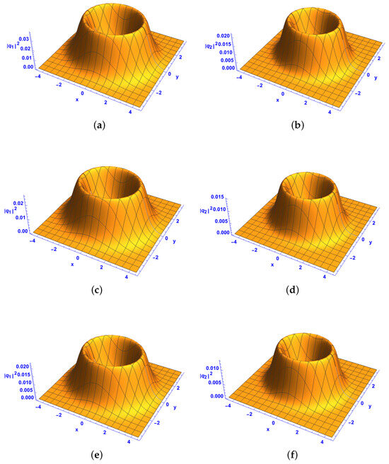
Figure 1. Intensity of the first-order bright–bright-like extreme wave solutions (37) and (38) under conditions (34)–(36) at $t=15$ and $z=1$, with (a,c,e) component $|q_1{|}^2$ and (b,d,f) component $|q_2{|}^2$. ${\beta }_0=0.5,{\beta }_3=0.15,\nu =0.8,l_0=0.4,p=2,n=3,k_0=0.3,g=0.5,a_{10}=0.15,b_{10}=0.2,$ $b_{20}=0.25$, $K=1,l=1,q=1,C_1=0.3-0.45i,C_3=0.4+0.25i,C_4={\displaystyle \frac{1}{2}},C_5={\displaystyle \frac{1}{3}},{ϵ}_{11}=1,$${ϵ}_{12}=1.25$, $\epsilon =1,G=1,P=1.25+0.75i,Q=1.35+0.85i$, with different gain parameters ${\mathsf{\Gamma }}_{1c}$ with (a,b) ${\mathsf{\Gamma }}_{1c}=0.1$, (c,d) ${\mathsf{\Gamma }}_{1c}=1.5$, and (e,f) ${\mathsf{\Gamma }}_{1c}=2$.

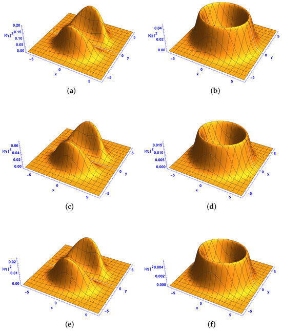
Figure 2. Intensity of the first-order bright–bright-like extreme wave solutions (37) and (38) under conditions (34)–(36) at $t=15$ and $z=1,$ with (a,c,e) component $|q_1{|}^2$ and (b,d,f) component $|q_2{|}^2.$ ${\beta }_0=0.5,{\beta }_3=0.5,\nu =0.8,l_0=0.5,p=0,n=1,k_0=0.4,g=0.3,a_{10}=0.15,b_{10}=0.18$, $b_{20}=0.2$, $K=1,l=0,q=1,C_1=2,C_3=2.2,C_4={\displaystyle \frac{1}{2}},C_5={\displaystyle \frac{1}{3}},{ϵ}_{11}=2,{ϵ}_{12}=2,\epsilon =1,$ $G=1$, $P=1,Q-1.2,$ with different gain parameters ${\mathsf{\Gamma }}_{1c}$ with (a,b) ${\mathsf{\Gamma }}_{1c}=0.1$, (c,d) ${\mathsf{\Gamma }}_{1c}=1$, and (e,f) ${\mathsf{\Gamma }}_{1c}=2$.

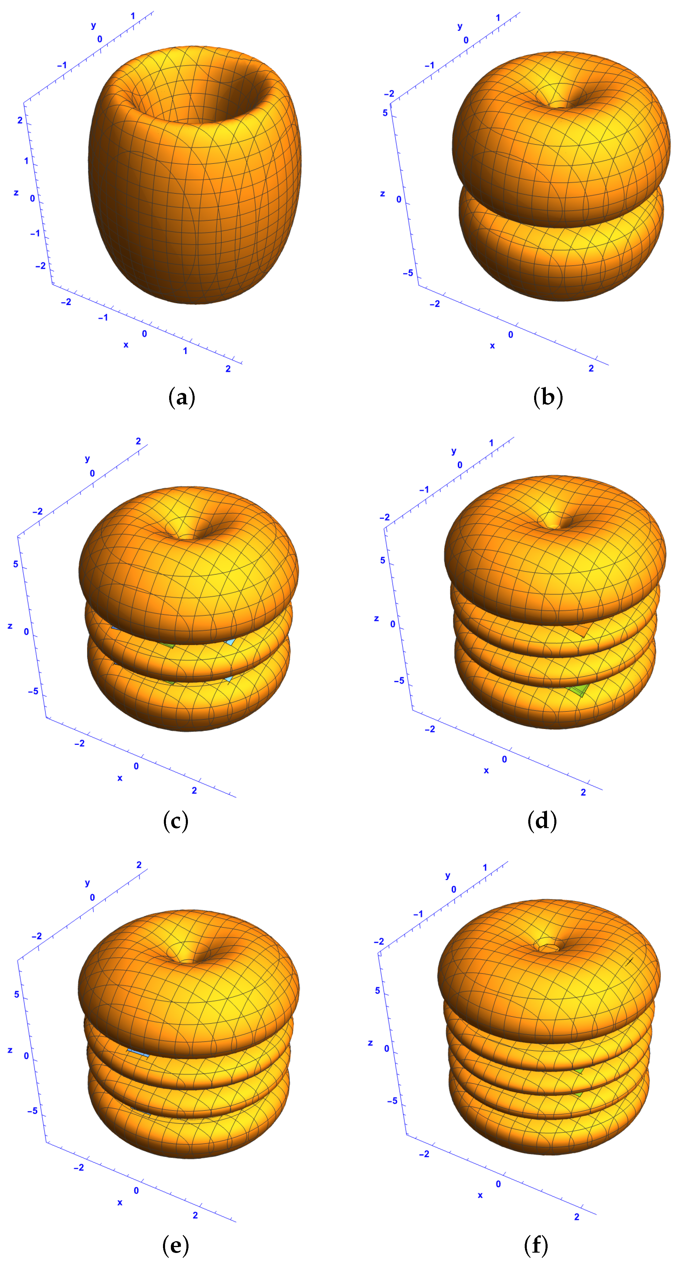
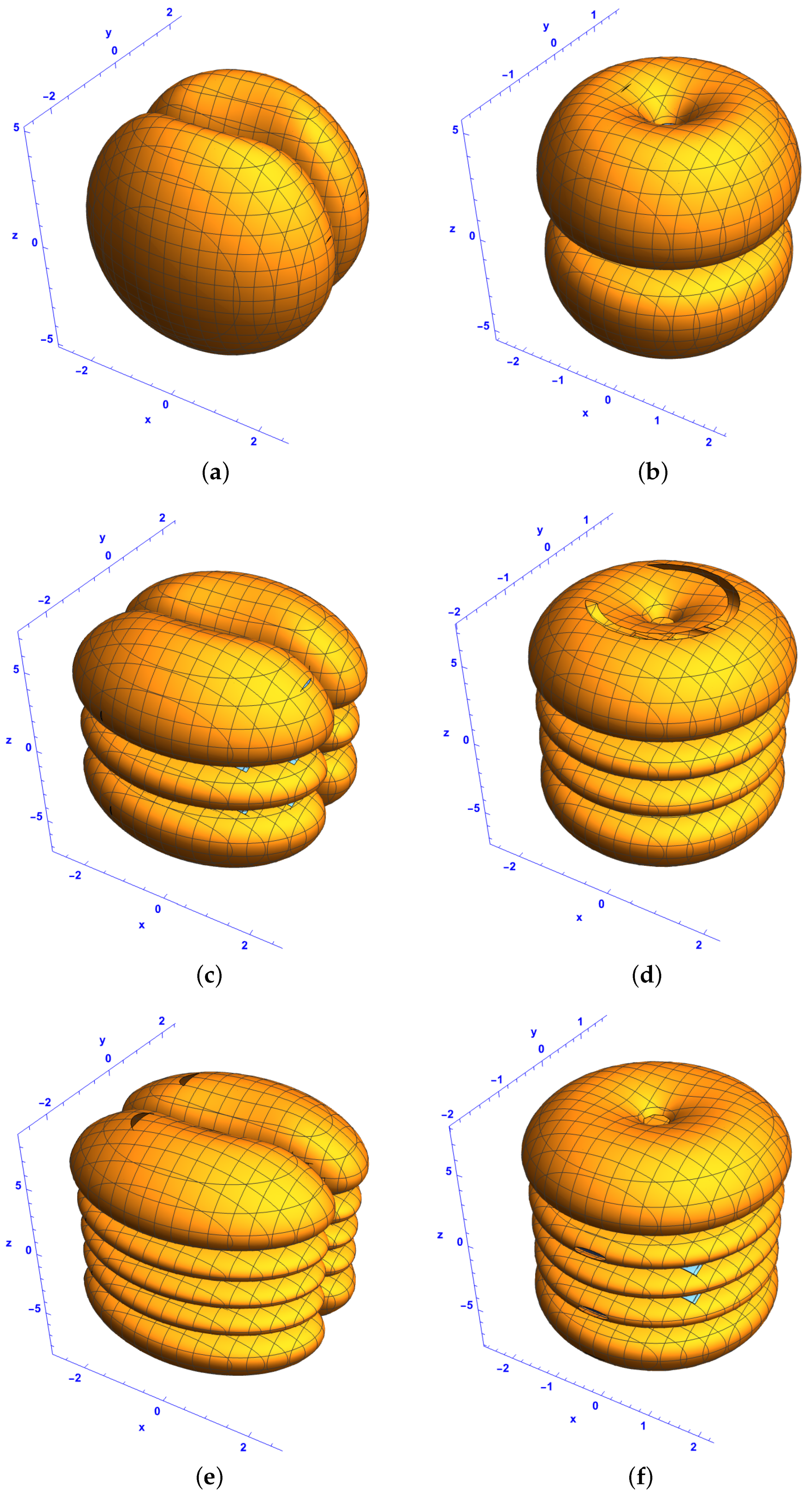
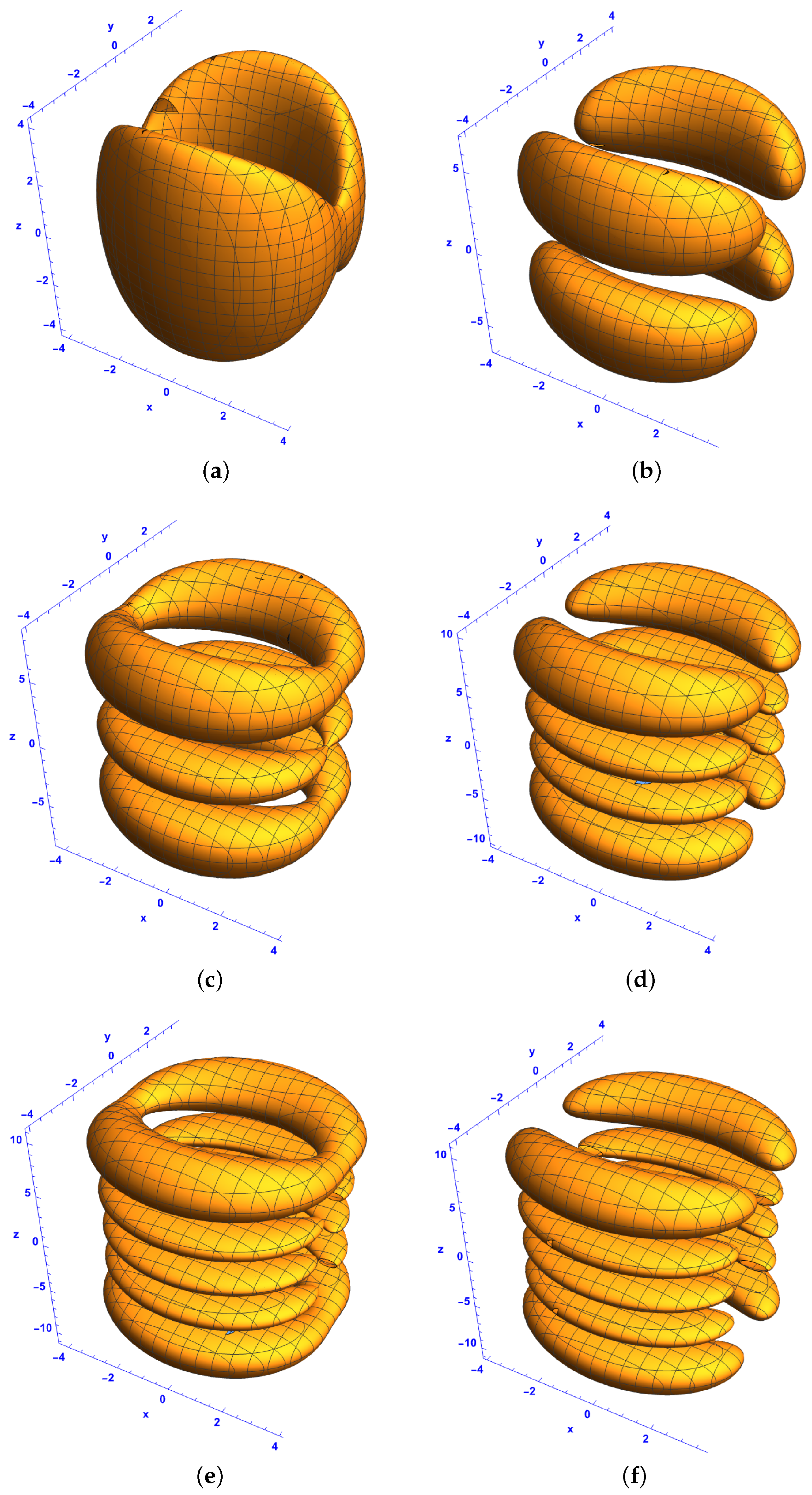
We can explore some localized structures by varying l and q. For $l=1$ and $q=1$, Gaussian soliton clusters can be formed, as shown in Figure 3. Notably, increasing the Hermite parameters p and n adds layers to these soliton clusters along the z-axis. The number of layers in the z-direction is given by $p+1$ and $n+1$, as illustrated in Figure 3a–f. In Figure 3a,c,e, the isosurface component $|q_1{|}^2$ is depicted, while Figure 3b,d,f show the isosurface component $|q_2{|}^2$. These multipole patterns reveal symmetric structures: a hollow cylinder and a pair of flat tori appear in Figure 3a and Figure 3b for $p=0$ and $n=1,$ respectively. A three-layer and a four-layer flat torus are shown in Figure 3c and Figure 3d for $p=2$ and $n=3$, respectively, while a four-layer and a five-layer flat torus are illustrated in Figure 1f and Figure 3e for $p=3$ and $n=4$, respectively.

Figure 3. Isosurface plots of the first-order bright–bright-like extreme wave solutions (37) and (38) under conditions (34)–(36) in the $xyz$ space at $t=2,$ with (a,c,e) component $|q_1{|}^2$ and (b,d,f) component $|q_2{|}^2.$ ${\beta }_0=0.5,{\beta }_3=0.15,\nu =0.8,l_0=0.4,k_0=0.3,g=0.5,a_{10}=0.15,b_{10}=0.2,b_{20}=0.25,$ $K=1$, ${\mathsf{\Gamma }}_{1c}=1.5,l=1,q=1,C_1=0.3-0.45i,C_3=0.4+0.25i,C_4={\displaystyle \frac{1}{2}},C_5={\displaystyle \frac{1}{3}},{ϵ}_{11}=1,$ ${ϵ}_{12}=1.25$, $\epsilon =1,G=1,P=1.25+0.75i,Q=1.35+0.85i$, with different Hermite parameters p and n: (a,b) $p=0$ and $n=1$, (c,d) $p=2$ and $n=3$, and (e,f) $p=3$ and $n=4$.

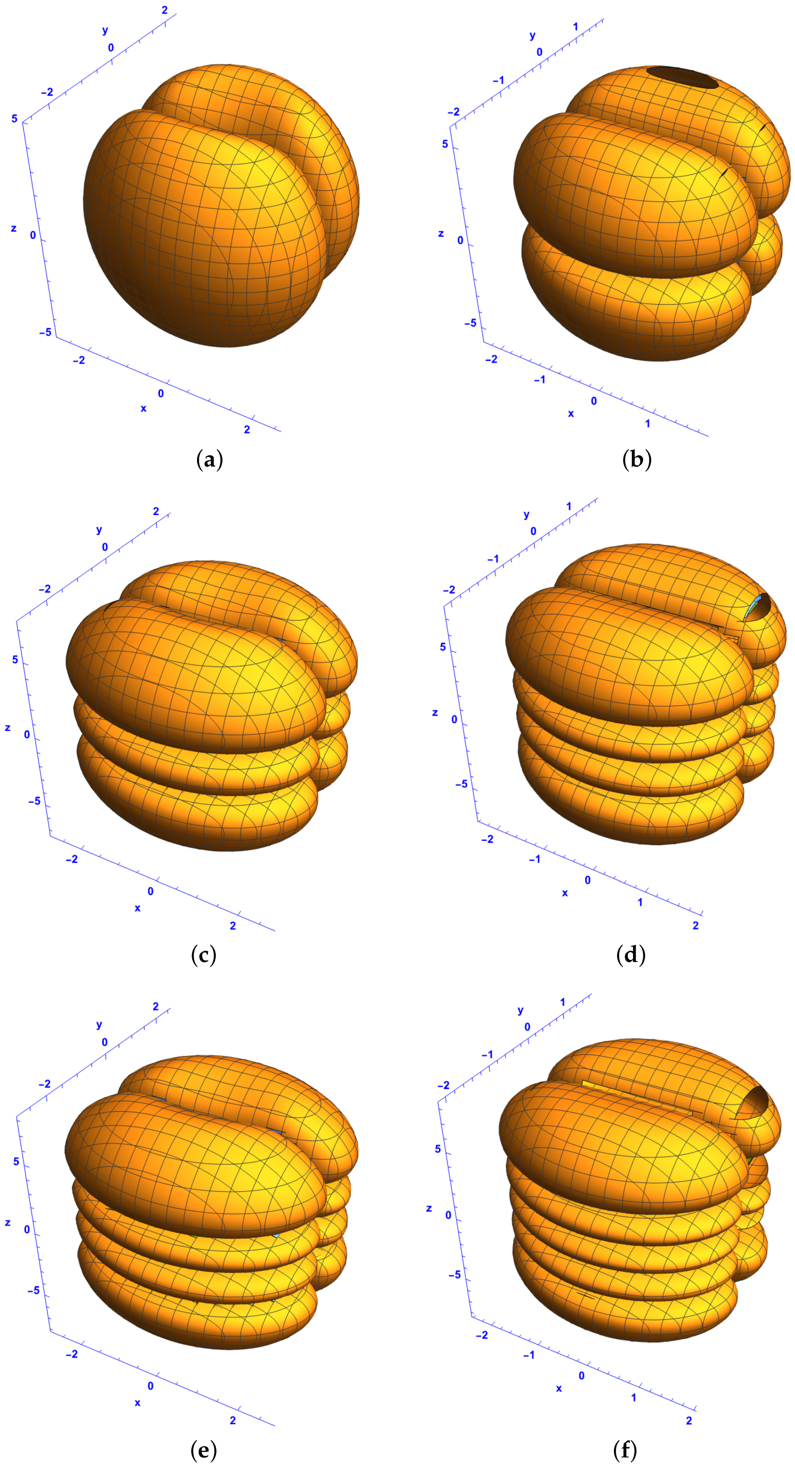
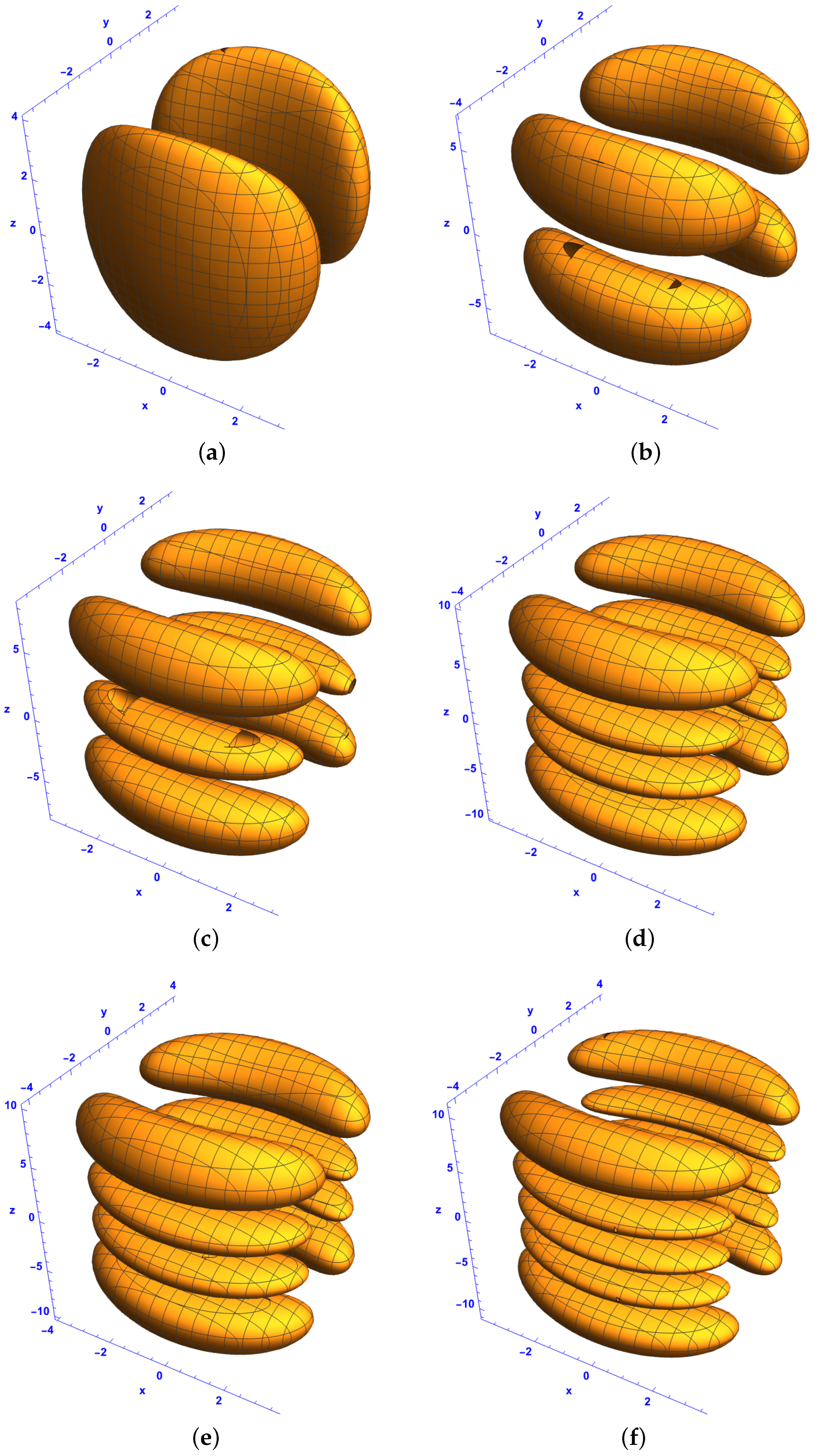
When $l=0$ and $q=1$, a different family of Gaussian soliton clusters is observed, as shown in Figure 4. For $p=0$ and $n=1$, Figure 4a and Figure 4b display two ellipsoids symmetrically arranged on either side of the plane $y=0$ and a pair of flat tori, respectively. For $p=2$ and $n=3$, Figure 4c,d show three ellipsoids symmetrically positioned around the plane $y=0$ and a three-layer flat torus. Finally, for $p=4$ and $n=4$, Figure 4e and Figure 4f show five ellipsoids arranged in pairs symmetrically distributed on either side of the plane $y=0$ and five flat tori, respectively. When $l=1$ and $q=0$, a different family of Gaussian soliton clusters is depicted in Figure 5. For $p=0$ and $n=1$, Figure 5a and Figure 5b show a pair of ellipsoids and two pairs of ellipsoids symmetrically arranged on either side of the plane $y=0$, respectively. For $p=2$ and $n=3$, Figure 5c,d show three ellipsoids arranged in pairs and four ellipsoids arranged in pairs symmetrically positioned around the plane $y=0$. For $p=4$ and $n=4$, Figure 5e and Figure 5f show four ellipsoids arranged in pairs and five ellipsoids arranged in pairs symmetrically distributed on either side of the plane $y=0$, respectively. Figure 3a,b show a hollow cylinder and a pair of flat tori for $p=0$ and $n=1$. Figure 3c,d show a three-layer and a four-layer flat torus for $p=2$ and $n=3$. Figure 3e,f show four-layer and five-layer flat tori for $p=3$ and $n=4$. The transition from a ring-like structure (as shown in Figure 3) to ellipsoidal clusters suggests a reconfiguration of soliton interactions due to the change in the parameter l. The presence of multiple ellipsoid structures highlights strong localization effects, which play a crucial role in the formation of extreme wave patterns. Unlike the flat torus structures in Figure 3 and Figure 4, Figure 5 emphasizes the ellipsoidal formations that emerge due to changes in q. The shift from ring-like solitons to clustered soliton pairs reflects how parameter variations impact wave coherence and stability.

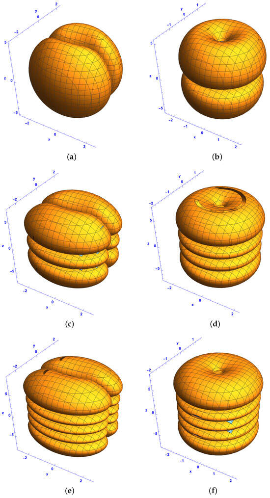
Figure 4. Isosurface plots of the first-order bright–bright-like extreme wave solutions (37) and (38) under conditions (34)–(36) in the $xyz$ space at $t=2$ for (a,c,e) component $|q_1{|}^2$ and (b,d,f) component $|q_2{|}^2$ for $l=0$ and $q=1$, with different Hermite parameters p and n: (a,b) $p=0$ and $n=1$, (c,d) $p=2$ and $n=3$, and (e,f) $p=4$ and $n=4$. The rest of the parameters are the same as in Figure 4.

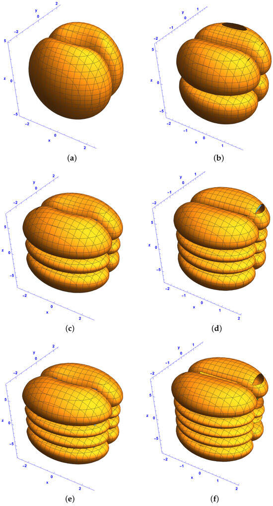
Figure 5. Isosurface plots of the first-order bright–bright-like extreme wave solutions (37) and (38) under conditions (34)–(36) in the $xyz$ space at $t=2$ for (a,c,e) component $|q_1{|}^2$ and (b,d,f) component $|q_2{|}^2$ for $l=0$ and $q=0$, with different Hermite parameters p and n: (a,b) $p=0$ and $n=1$, (c,d) $p=2$ and $n=3$, and (e,f) $p=3$ and $n=4$. The rest of the parameters are the same as in Figure 4.

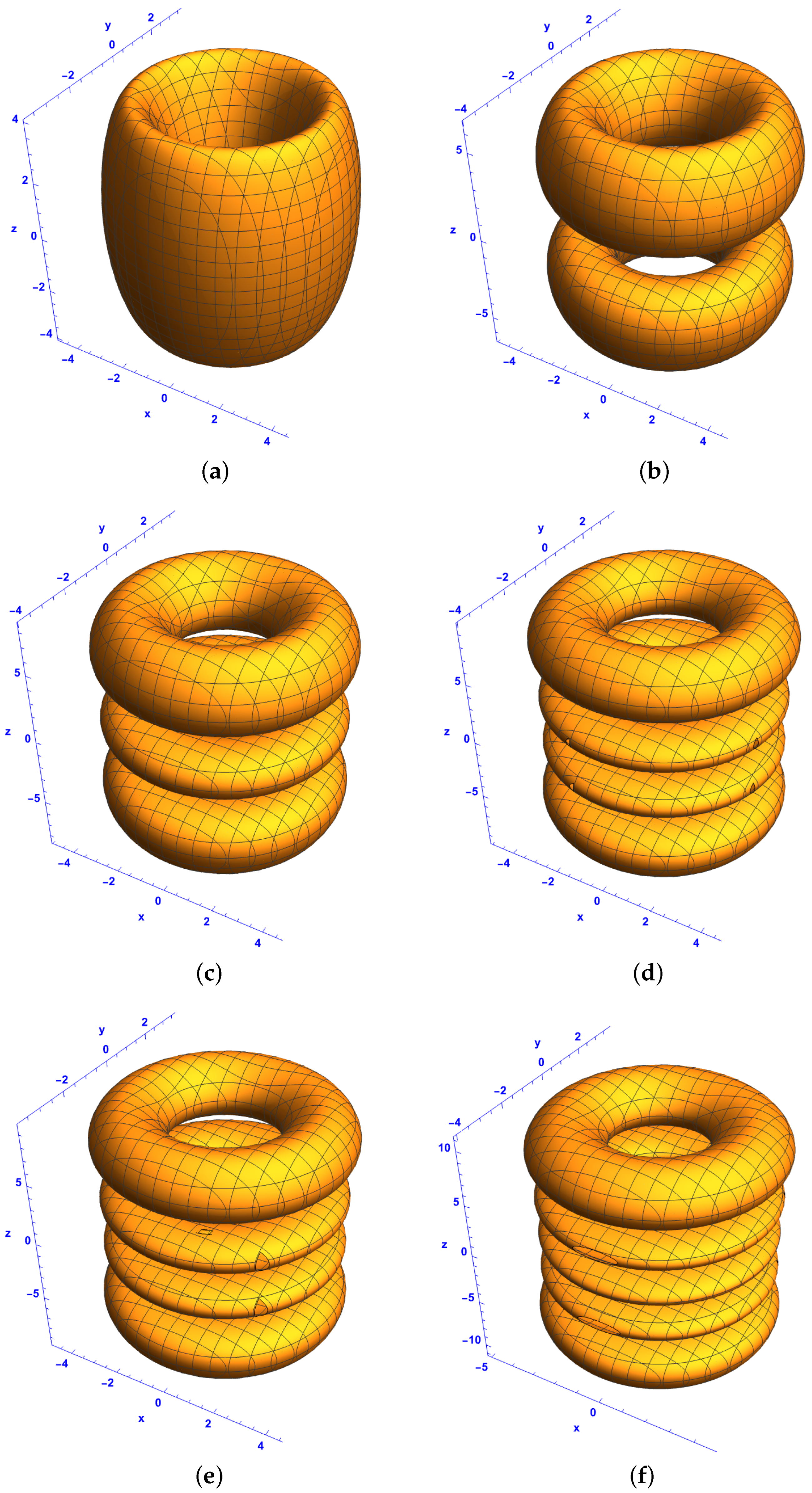
In the following, we examine the PNL characteristics of the bright–bright soliton structure in the system described by (39) for $t=2$ in the $xyz$ coordinate system. Figure 6 displays Gaussian multipole solitons when $l=0$ and $q=0$. Specifically, the figure shows pairs of ellipsoids symmetrically distributed on both sides of the plane $y=0$. In Figure 6a and Figure 6b, which depict $|q_1{|}^2$ and $|q_2{|}^2$, respectively, a pair of ellipsoids appears in each case when $p=0$ and $n=1$. Figure 6c and Figure 6d show three ellipsoids arranged in pairs and four ellipsoids arranged in pairs corresponding to $p=2$ and $n=3,$ respectively. Similarly, four ellipsoids arranged in pairs and five ellipsoids arranged in pairs are observed for $p=3$ and $n=4.$ All these structures exhibit symmetry about the plane $y=0$. In the $xyz$ space, cylinder-like and ring-like structures are shown in Figure 7 for $l=1$ and $q=1$. Specifically, Figure 7a and Figure 7b display a cylinder-like structure and a two-layer ring-like structure corresponding to $p=0$ and $n=1,$ respectively. When comparing Figure 7c and Figure 7d with Figure 7e and Figure 7f, we observe that the number of layers in the ring structure along the z-direction corresponds to $p+1$ and $n+1$ for the Hermite parameters p and n, respectively. For instance, Figure 7c,d illustrate a three-layer and a four-layer ring for $p=2$ and $n=3,$ while Figure 7e,f show a four-layer and a five-layer ring for $p=3$ and $n=4$. To explore the spatiotemporal localization and characteristics of multipole structures, we present isosurface plots in Figure 8 for $l=0$ and $q=1$. Using the system described by Equation (21), Figure 8 depicts isosurface plots in the $xyz$ space at $t=2$, illustrating the first-order ring-like extreme waves. The figure displays ellipsoid-like structures symmetrically distributed on both sides of the plane $y=0$ and ring-like structures. Specifically, Figure 8a and Figure 8b show a pair of ellipsoids and a pair of ring-like structures for $p=0$ and $n=1,$ respectively. Figure 8c and Figure 8d depict three ellipsoids arranged in pairs and a four-layer ring-like structure for $p=2$ and $n=3$, respectively. Similarly, Figure 8e,f illustrate five ellipsoids arranged in pairs and a five-layer ring-like structure for $p=4$ and $n=4$. Figure 9 plots multipole soliton clusters for $l=1/2$ and $q=1/3$, showing symmetric structures on both sides of the plane $y=0.$ In Figure 9a,c,e with $|q_1{|}^2$ and Figure 9b,d,f with $|q_2{|}^2$, the multipole solitons are symmetrically arranged around the plane $y=0$. Specifically, Figure 9a,b show a single structure and a pair of ellipsoids for $p=0$ and $n=1$. Figure 9c,d show a three-layer structure and four ellipsoids arranged in pairs for $p=2$ and $n=3$. Similarly, Figure 9e,f display a five-layer structure and five ellipsoids arranged in pairs for $p=4$ and $n=4$. The ellipsoidal formations observed in Figure 6 indicate a significant localization effect due to the interplay of diffraction and nonlinearity, restricting soliton dispersion in the transverse plane. Unlike the ring-like structures in Figure 7 and Figure 8, Figure 6 focuses on ellipsoidal solitons, which are more confined and structured due to the chosen values of l and q. This confirms that nonlocality in the z-direction plays a role in determining the shape and evolution of these solitonic structures. Figure 7 shows how increases in l and q transform solitons from compact ellipsoidal structures (as seen in Figure 6) to wider, ring-like formations. This transformation suggests that higher values of l and q promote radial soliton expansion, which allows soliton interactions to develop into complex topological structures. The transition from a cylinder-like structure to multi-ring solitons suggests a redistribution of energy across the solitonic wavefront. These solitons maintain coherence and do not disperse over time, demonstrating stability despite changes in diffraction and gain. Unlike Figure 6 and Figure 7, Figure 8 shows both ellipsoidal and ring-like solitons in the same setting. The nonlocal interactions along the z-direction observed in Figure 8 enhance the ring-like soliton properties, allowing the solitons to develop more intricate shapes over time. This differs from Figure 6, where solitons remain confined to an ellipsoidal shape, indicating that higher q values promote extended solitonic structures. Figure 9 reveals a transitional soliton regime, where localized soliton clusters evolve into more complex multipole formations. The fractional values of l and q introduce more intricate soliton arrangements, as opposed to the simpler symmetric structures in Figure 6, Figure 7 and Figure 8. Unlike the purely symmetric Gaussian solitons in Figure 6, the solitons in Figure 9 exhibit asymmetry and a multipole structure, confirming that fractional values of l and q introduce new solitonic interactions. The transformation observed in Figure 9 suggests that certain parameter choices lead to hybrid soliton formations, where individual solitons interact and form multipole structures.

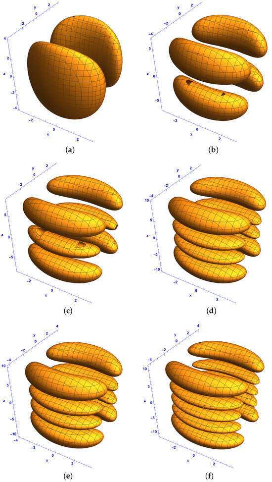
Figure 6. Isosurface plots of the first-order bright–bright-like extreme wave solutions (37) and (38) under conditions (34)–(36) in the $xyz$ space at $t=2$ for (a,c,e) component $|q_1{|}^2$ and (b,d,f) component $|q_2{|}^2.$ ${\beta }_0=0.5,{\beta }_3=0.5,\nu =0.8,l_0=0.5,p=0,n=1,k_0=0.4,g=0.3,a_{10}=0.15$, $b_{10}=0.18$, $b_{20}=0.2,K=1,{\mathsf{\Gamma }}_{1c}=0.5,l=0,q=0,C_1=2,C_3=2.2,C_4={\displaystyle \frac{1}{2}},C_5={\displaystyle \frac{1}{3}},{ϵ}_{11}=2,{ϵ}_{12}=2,$ $\epsilon =1$, $G=1,P=1$, and $Q-1.2$, with different Hermite parameters p and n: (a,b) $p=0$ and $n=1$, (c,d) $p=2$ and $n=3$, and (e,f) $p=3$ and $n=4$.

Figure 7. Isosurface plots of the first-order bright–bright-like extreme wave solutions (37) and (38) under conditions (34)–(36) in the $xyz$ space at $t=2$ for (a,c,e) component $|q_1{|}^2$ and (b,d,f) component $|q_2{|}^2$ for $l=1$ and $q=1$, with different Hermite parameters p and n: (a,b) $p=0$ and $n=1$, (c,d) $p=2$ and $n=3$, and (e,f) $p=3$ and $n=4$. The rest of the parameters are the same as in Figure 6.

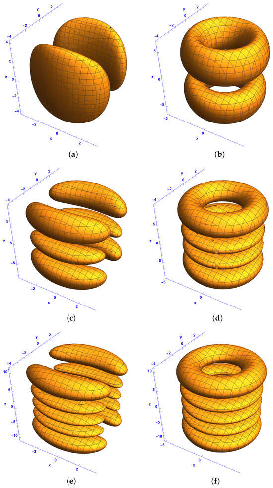
Figure 8. Isosurface plots of the first-order bright–bright-like extreme wave solutions (37) and (38) under conditions (34)–(36) in the $xyz$ space at $t=2$ for (a,c,e) component $|q_1{|}^2$ and (b,d,f) component $|q_2{|}^2$ for $l=0$ and $q=1$, with different Hermite parameters p and n: (a,b) $p=0$ and $n=1$, (c,d) $p=2$ and $n=3$, and (e,f) $p=4$ and $n=4$. The rest of the parameters are the same as in Figure 6.

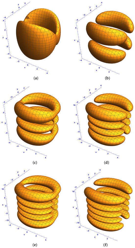
Figure 9. Isosurface plots of the first-order bright–bright-like extreme wave solutions (37) and (38) under conditions (34)–(36) in the $xyz$ space at $t=2$ for (a,c,e) component $|q_1{|}^2$ and (b,d,f) component $|q_2{|}^2$ for $l=1/2$ and $q=1/3$ with different Hermite parameters p and n: (a,b) $p=0$ and $n=1$, (c,d) $p=2$ and $n=3$, and (e,f) $p=4$ and $n=4$. The rest of the parameters are the same as in Figure 6.

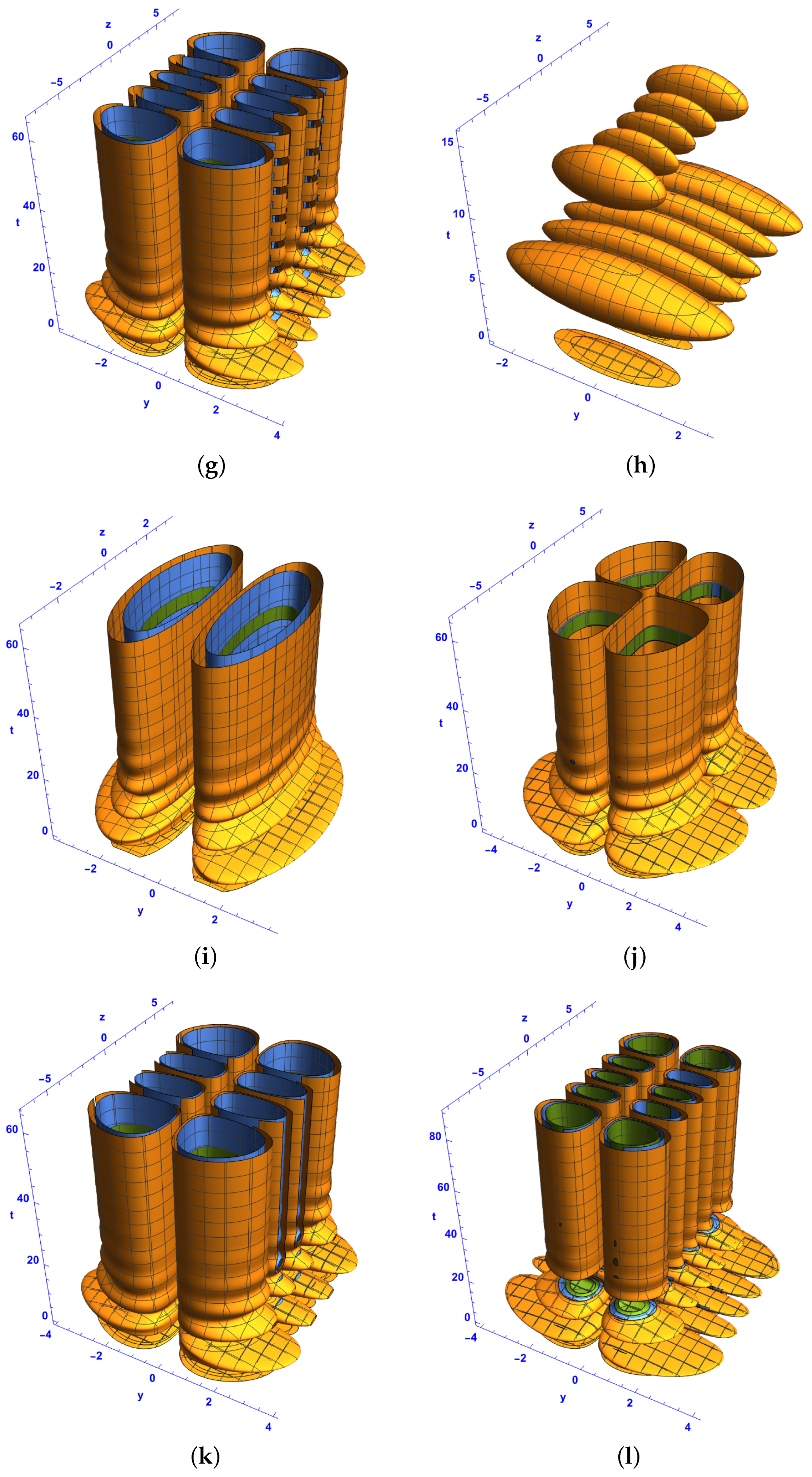
For our system, as described by Equation (39), where diffraction, PNL nonlinearity, and gain decay exponentially while the chirp and phases remain constant, Figure 10 displays isosurface plots that represent the one-soliton bright–bright monster waves in the $yzt$-spacetime domain, in which the coefficients $C_i$ (for i = 1, 2, 3, 4), P, and Q are complex. Similarly, Figure 11 presents isosurface plots of the extreme waves in the same spacetime context, but with real values for the coefficients $C_i$, P, and Q. For a fixed gain value ${\mathsf{\Gamma }}_{1c}$, an increase in the Hermite parameters p and n along the z-axis leads to an increase in the number of layers within the extreme wave structures. It is also evident in Figure 10b,d,f,h that the gain progressively reduces the size of the structures. Specifically, as time increases, the layers within these structures become smaller, as observed in these figures.

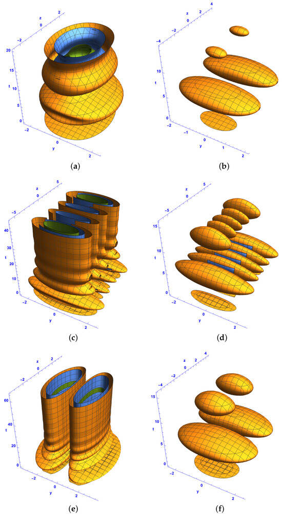
Figure 10. Isosurface plots of the first-order bright–bright-like extreme wave solutions (37) and (38) under conditions (34)–(36) in the $yzt$ spacetime at $x=3,$ for $l=1$ and $q=1$ (a–d), $l=0$ and $q=1$ (e–h), and $l=0$ and $q=0$ (i–l) with different Hermite parameters p and n: (a,b,e,f,i,j) $p=0$ and $n=1$, (c,d,k,l) $p=3$ and $n=4$, and (g,h) $p=4$ and $n=4$. The rest of the parameters are ${\beta }_0=0.5,{\beta }_3=0.15,\nu =0.8,{\mathsf{\Gamma }}_{1c}=1.5,l_0=0.4,k_0=0.3,g=0.5,a_{10}=0.15,b_{10}=0.2,$ $b_{20}=0.25$, $K=1,C_1=0.3-0.45i,C_3=0.4+0.25i,C_4={\displaystyle \frac{1}{2}},C_5={\displaystyle \frac{1}{3}},{ϵ}_{11}=1,{ϵ}_{12}=1.25,\epsilon =1,G=1$, $P=1.25+0.75i$, and $Q=1.35+0.85i$.

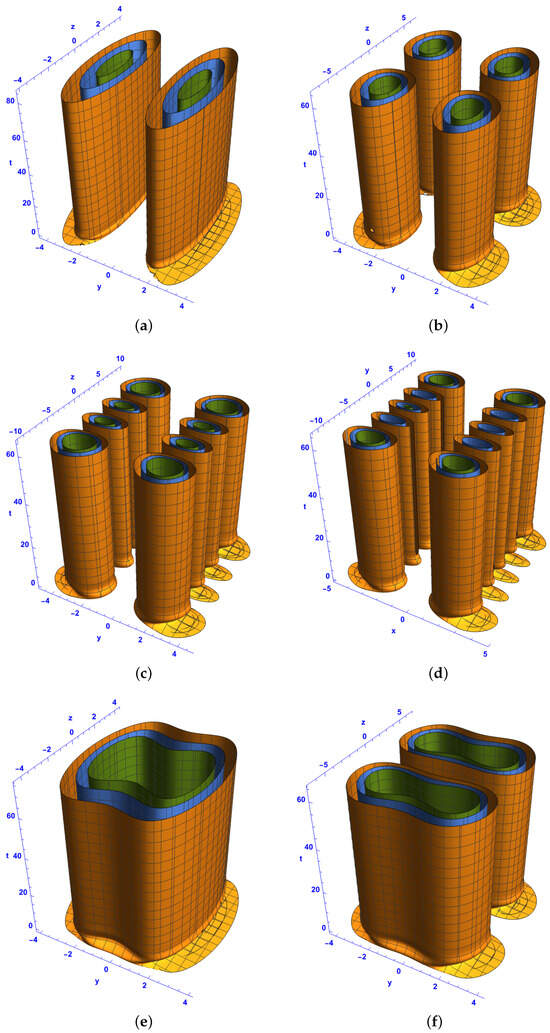
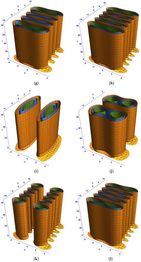
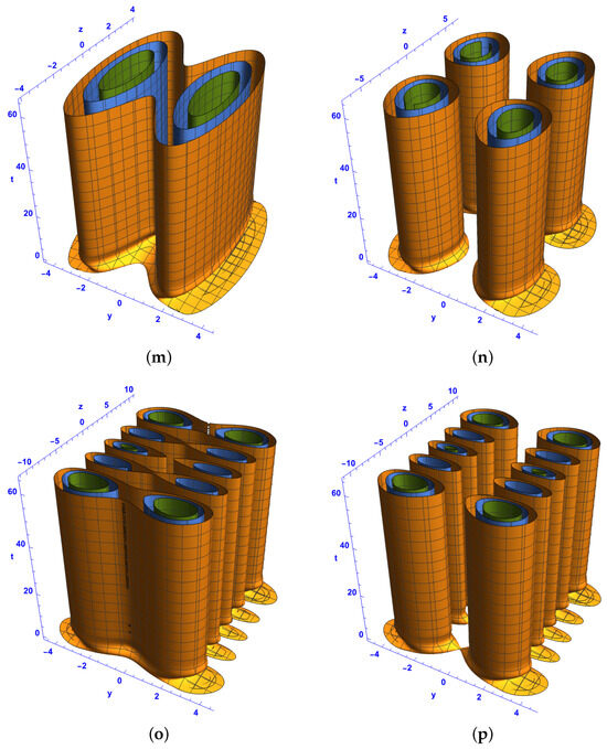
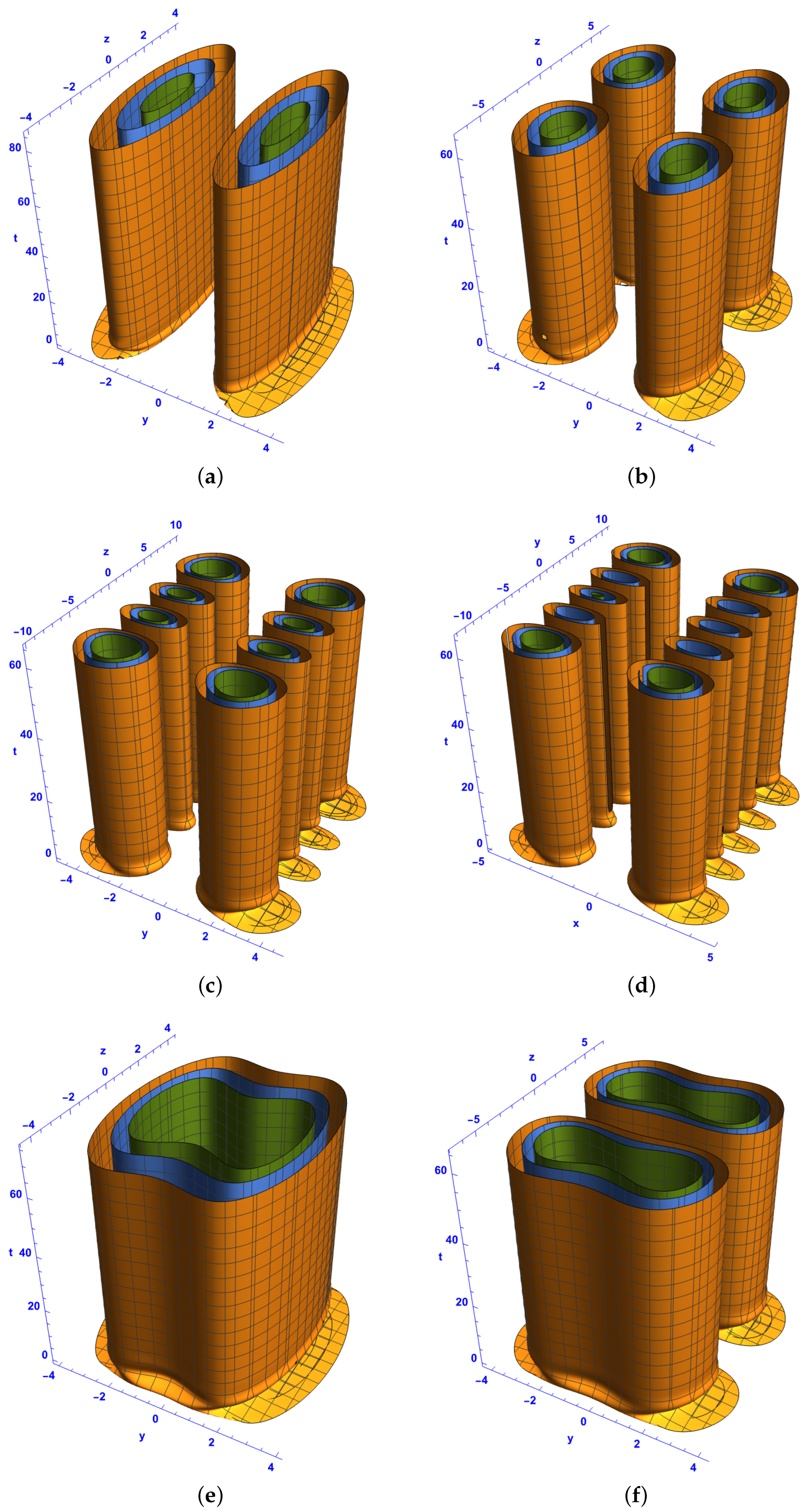
Figure 11. Isosurface plots of the first-order bright–bright-like extreme wave solutions (37) and (38) under conditions (34)–(36) in the $yzt$ spacetime at $x=3,$ for $l=0$ and $q=0$ (a–d), $l=1$ and $q=1$ (e–h), $l=0$ and $q=1$ (i–l), and $l=1/2$ and $q=1/3$ (m–p), with different Hermite parameters p and n: (a,b,e,f,i,j,m,n) $p=0$ and $n=1$, (c,d,g,h) $p=3$ and $n=4$, and (k,l,o,p) $p=4$ and $n=4$. The rest of the parameters are ${\beta }_0=0.5,{\beta }_3=0.5,\nu =0.8,l_0=0.5,k_0=0.4,$ $g=0.3$, $a_{10}=0.15,b_{10}=0.18,b_{20}=0.2,K=1,{\mathsf{\Gamma }}_{1c}=0.5,C_1=2,C_3=2.2,C_4={\displaystyle \frac{1}{2}},C_5={\displaystyle \frac{1}{3}},$ ${ϵ}_{11}=2$, ${ϵ}_{12}=2,\epsilon =1,G=1,P=1,$ and $Q=1.2$.

• Analysis of Figure 10 (Bright–Bright Monster Waves in the $yzt$-Spacetime)

Figure 10 illustrates isosurface plots of the first-order bright–bright monster waves in the $yzt$-spacetime domain for different values of l and q. These figures analyze the impact of the gain parameter ${\mathsf{\Gamma }}_{1c}$, the Hermite parameters p and n, and their effects on the soliton structures.

• Effect of Hermite Parameters p and n:

Increasing p and n leads to a greater number of soliton layers along the z-axis. This aligns with previous observations from Figure 1, Figure 2, Figure 3, Figure 4, Figure 5, Figure 6, Figure 7, Figure 8 and Figure 9, where the number of soliton layers was determined by $p+1$ and $n+1$. For example, in Figure 10a,b, where $p=0$, and $n=1$, a single-layer bright–bright soliton structure is observed. As p and n increase in Figure 10c,d (p = 3, n = 4), multiple layers emerge, forming a more complex soliton pattern.

• Influence of Gain ${\mathsf{\Gamma }}_{1c}$:

Higher gain values reduce the size of the soliton structures over time. This behavior is consistent with observations from previous figures.

Figure 10b,d,f,h confirm this by showing how the structures contract as time progresses, leading to soliton compression.

• Topological Variations with Different l and q:

The choice of l and q affects the structure of the solitons.

For $l=1$ and $q=1$ (Figure 10a,b), the solitons exhibit a ring-like structure in the $yzt$-spacetime. For $l=0$ and $q=1$ (Figure 10e,f), a more elliptical structure is observed. When $l=0$ and $q=0$ (Figure 10i,j), the soliton structures become elongated.

• Analysis of Figure 11 (Bright–Bright Monster Waves in $yzt$-Spacetime with Real Coefficients)

Figure 11 presents isosurface plots similar to those in Figure 10 but under the constraint that the coefficients $C_i$, P, and Q are real.

• Structural Differences from Figure 10:

Unlike Figure 10, where complex coefficients result in asymmetric or irregular soliton patterns, Figure 11 exhibits more structured and symmetric soliton formations. The structures are more evenly distributed along the z-axis due to the absence of imaginary phase shifts.

• Effect of l and q:

For $l=0$ and $q=0$ (Figure 11a,b), the solitons exhibit a localized, compressed form. For $l=1$ and $q=1$ (Figure 11e,f), ring-like formations appear, similar to those in Figure 10. In Figure 11m,n, where $l=1/2$ and $q=1/3$, the soliton structure appears as a hybrid of ring-like and ellipsoid formations.

• Impact of Real Coefficients:

Since the coefficients are real, phase oscillations are reduced, which leads to more stable soliton structures. The evolution of these solitons is smoother than those in Figure 10.

4. Conclusions

In this study, we addressed key gaps in understanding extreme wave solutions in (3+1)-dimensional partially nonlocal media. By analyzing a (3+1)-dimensional coupled nonlinear Schrödinger (NLS) system influenced by linear and harmonic potentials, as well as gain and loss effects, we have significantly advanced the field. Our application of Lens transformation enabled us to simplify the system to a (2+1)-dimensional constant-coefficient model, allowing the derivation of analytical solutions for ring-like bright–bright vector two-component solitons using Hirota’s bilinearization method. This approach not only offers novel insights into the behavior and evolution of extreme waves but also enhances our understanding of their dynamics under different dispersion and nonlinearity conditions.

4.1. Key Findings and Contributions

Impact of Gain and Loss:

The inclusion of gain and loss terms significantly affects the propagation of these waves. As shown in Figure 1 and Figure 2, increasing ${\mathsf{\Gamma }}_{1c}$ leads to intensity reduction and soliton compression, emphasizing the crucial role of gain management in controlling soliton behavior within nonlinear, partially nonlocal media.

Role of Hermite Parameters and Structural Evolution:

Figure 3, Figure 4 and Figure 5 confirm that Hermite parameters p and n determine soliton layering, while l and q govern the overall soliton structure and localization patterns.

Figure 6, Figure 7, Figure 8 and Figure 9 highlight the diverse soliton formations, emphasizing the role of PNL nonlinearity, diffraction, and gain in shaping soliton behavior.

Classification of Soliton Structures:

Figure 6 presents localized Gaussian multipole solitons, maintaining strong symmetry around $y=0$, with ellipsoidal soliton formations shaped by Hermite parameters. Figure 7 transitions into cylinder-like and multi-ring solitons, demonstrating how higher values of l and q promote radial expansion. Figure 8 reveals both ellipsoidal and ring-like solitons, suggesting a hybrid regime where localized and extended solitons coexist. Figure 9 introduces multipole soliton clusters, showing how fractional values of l and q lead to intricate solitonic formations.

Soliton Dynamics in Spatiotemporal Framework:

Figure 10 and Figure 11 extend our previous results by exploring soliton evolution in the yzt-spacetime domain. The number of soliton layers increases with p and n, while higher ${\mathsf{\Gamma }}_{1c}$ leads to soliton contraction over time. Figure 10 demonstrates asymmetric soliton behavior due to complex coefficients, whereas Figure 11 shows more structured soliton formations when real coefficients are used.

These findings further confirm the ability to manipulate bright–bright monster waves using Hermite parameters and gain modulation.

4.2. Broader Implications and Future Directions

Our investigation underscores the controllability of soliton behavior in partially nonlocal media, particularly ring-like and cylinder-like extreme waves in optical and matter-wave systems. By carefully selecting diffraction, linear, parabolic (in the x-direction), and PNL nonlinearity coefficients, we demonstrate precise control over soliton formation and evolution. This nuanced control mechanism opens avenues for tailored applications across diverse fields, particularly in nonlinear optics, Bose–Einstein condensates, and optical communication systems. Future work will extend these findings by exploring more complex soliton interactions, refining wave management strategies, and investigating integrability properties within the PNL-NLS framework.

This paper extends the theoretical framework of extreme wave solutions by identifying and characterizing new soliton structures in partially nonlocal media. The results offer deeper insights into wave localization, soliton interactions, and parameter-driven soliton clustering. Our findings provide a foundation for future research into high-dimensional wave phenomena and their practical applications, paving the way for new soliton-based technologies in nonlinear optical systems and quantum wave dynamics.

References

- Mitchell, D.J.; Snyder, A.W. Soliton dynamics in a nonlocal medium. J. Opt. Soc. Am. B 1999, 16, 236. [Google Scholar] [CrossRef]
- Zhu, H.P.; Chen, L.; Chen, H.Y. Hermite–Gaussian vortex solitons of a (3+1)-dimensional partially nonlocal nonlinear Schrödinger equation with variable coefficients. Nonlinear Dyn. 2016, 85, 1913. [Google Scholar] [CrossRef]
- Dai, C.Q.; Wang, Y.; Liu, J. Spatiotemporal Hermite-gaussian solitons of a (3+1)-dimensional partially nonlocal nonlinear Schrödinger equation. Nonlinear Dyn. 2016, 84, 1157. [Google Scholar] [CrossRef]
- Dai, C.Q.; Zhang, J.F. Controlling effects of vector and scalar crossed doubled-Ma breathers in a partially nonlocal nonlinear medium with a linear potential. Nonlinear Dyn. 2020, 100, 1621. [Google Scholar] [CrossRef]
- Liu, Q. Analytical matter wave solutions of a (2+1)-dimensional partially nonlocal distributed-coefficient Gross-Pitaevskii equation with a linear potential. Optik 2020, 200, 163434. [Google Scholar] [CrossRef]
- Wu, H.Y.; Jiang, L.H. Vortex soliton solutions of a (3+1)-dimensional Gross-Pitaevskii equation with partially nonlocal distributed coefficient under a linear potential. Nonlinear Dyn. 2020, 101, 2441. [Google Scholar] [CrossRef]
- Wu, H.Y.; Jiang, L.H. 3D partially nonlocal ring-like Kuznetsov-Ma and Akhmediev breathers of NLS model with different diffractions under a linear potential. Chaos Solitons Fractals 2024, 182, 114862. [Google Scholar] [CrossRef]
- Chen, Y.X.; Xu, F.Q.; Hu, Y.L. Excitation control for three-dimension Peregrine solution and combined breather of a partially nonlocal variable-coefficient Schrödinger equation. Nonlinear Dyn. 2019, 95, 1957. [Google Scholar] [CrossRef]
- Yang, J.; Zhu, Y.; Qin, W.; Wang, S.; Dai, C.Q.; Li, J. Higher dimensional soliton structures of a variable-coefficient Gross-Pitaevskii equation with the partially nonlocal nonlinearity under a harmonic potential. Nonlinear Dyn. 2022, 108, 2551. [Google Scholar] [CrossRef]
- Chen, L.Y.; Yu, H.Y.; Jiang, L.H. Ring-like two breather structures of a partially nonlocal NLS system with different two-directional diffractions under a parabolic potential. Chaos Solitons Fractals 2024, 178, 114330. [Google Scholar] [CrossRef]
- Zhu, Y.; Yang, J.; Chen, Z.; Qin, W.; Li, J. Ring-like partially nonlocal extreme wave of a (3+1)-dimensional NLS system with partially nonlocal nonlinearity and extreme potential. Chaos Solitons Fractals 2024, 182, 114750. [Google Scholar] [CrossRef]
- Zhu, Y.; Yang, Y.; Qin, W.; Wang, S.; Li, J. Ring-like double-breathers in the partially nonlocal medium with different diffraction characteristics in both directions under the external potential. Chaos Solitons Fractals 2024, 180, 114510. [Google Scholar] [CrossRef]
- Dai, C.Q.; Wang, Y.; Zhang, J.F. Managements of scalar and vector rogue waves in a partially nonlocal nonlinear medium with linear and harmonic potentials. Nonlinear Dyn. 2020, 102, 379. [Google Scholar] [CrossRef]
- Dai, C.Q.; Liu, J.; Fan, Y.; Yu, D.G. Two -dimensional localized Peregrine solution and breather excited in a variable-coefficient nonlinear Schrödinger equation with partial nonlocality. Nonlinear Dyn. 2017, 88, 1373. [Google Scholar] [CrossRef]
- Chen, X.X. Excitation manipulation of three-dimensional completely localized rogue waves in a partially nonlocal and inhomogeneous nonlinear medium. Nonlinear Dyn. 2019, 97, 177. [Google Scholar] [CrossRef]
- Wu, H.Y.; Jiang, L.H. Excitation management of (2+1)-dimensional breathers for a coupled partially nonlocal nonlinear Schrodinger equation with variable coefficients. Nonlinear Dyn. 2019, 95, 3401. [Google Scholar] [CrossRef]
- Wang, Y.Y.; Dai, C.Q.; Xu, Y.Q.; Zheng, J.; Fan, Y. Dynam- ics of nonlocal and localized spatiotemporal solitons for a partially nonlocal nonlinear Schrodinger equation. Nonlinear Dyn. 2018, 92, 1261. [Google Scholar] [CrossRef]
- Yang, J.; Zhu, Y.; Qin, W.; Wang, S.; Li, J. Spatiotemporal vector vortex and diploe solitons of a nonautonomous partially nonlocal coupled Gross-Pitaevskii equation with a linear potential. Results Phys. 2021, 30, 104860. [Google Scholar] [CrossRef]
- Chen, Y.X.; Xiao, X. Vector bright dark one-soliton and two-soliton of the coupled NLS model with the partially nonlocal nonlinearity in BEC. Optik 2022, 257, 168708. [Google Scholar] [CrossRef]
- Chen, Y.X.; Xiao, X. Vector soliton pairs for a coupled nonautonomous NLS model with partially nonlocal coupled nonlinearities under the external potentials. Nonlinear Dyn. 2022, 109, 2003. [Google Scholar] [CrossRef]
- Wu, H.; Jiang, L.H. Diverse excitations of two-component rogue waves for a nonautonomous coupled partially nonlocal nonlinear Schrodinger model under a parabolic potential. Nonlinear Dyn. 2022, 109, 1993. [Google Scholar] [CrossRef]
- Chen, L.; Zhu, H.P. Partially nonlocal bright-dark rogue waves and bright-bright rogue wave pairs of a vector nonlinear Schrodinger equation. Nonlinear Dyn. 2023, 111, 7699. [Google Scholar] [CrossRef]
- Zhu, H.P.; Chen, L. Vector dark-bright second-order rogue wave and triplets for a (3+1)-dimensional CNLSE with the partially nonlocal nonlinearity. Nonlinear Dyn. 2023, 111, 4673. [Google Scholar] [CrossRef]
- Chen, Y.X. Versatile excitations of 3D partially nonlocal bright-bright Peregrine quartets in a nonautonomous vector nonlinear Schrodinger equation under a parabolic potential. Nonlinear Dyn. 2023, 111, 11437. [Google Scholar] [CrossRef]
- Chen, Y.X. Diverse partially nonlocal bright-dark Peregrine three sisters excitations in a (3+1)-dimensional vector nonlinear Schrodinger equation. Results Phys. 2023, 51, 106706. [Google Scholar] [CrossRef]
- Zhu, H.P.; Xu, Y.J. High-dimensional vector solitons for a variable-coefficient partially nonlocal coupled Gross-Pitaevskii equation in a harmonic potential. Appl. Math. 2022, 124, 107701. [Google Scholar] [CrossRef]
- Zhu, H.P.; Xu, Y.J. High-dimensional vector two-component solitons of a nonautonomous partially nonlocal coupled NLS model in a linear and harmonic potential. Nonlinear Dyn. 2023, 111, 581. [Google Scholar] [CrossRef]
- Chen, Y.X. (3+1)-dimensional partial nonlocal ring-like bright-dark monster waves. Chaos Solitons Fractals 2024, 180, 114519. [Google Scholar] [CrossRef]
- Yomba, E. Ring/vortex-like extreme waves for variable-coefficient axially and partially nonlocal coupled nonlinear Schrödinger equations with different diffraction characteristics in transverse plane under influence of external potential and gain/loss. Nonlinear Dyn. 2024, 113, 7095–7120. [Google Scholar] [CrossRef]
- Yomba, E. Ring-like double-breathers in the partially nonlocal medium with different diffraction characteristics in both directions under the influence of external potential and gain/loss. Phys. Lett. A 2025, 536, 130293. [Google Scholar] [CrossRef]
- Mitschke, F.; Hause, A.; Mahnke, C. Solitons in fibers with loss beyond small perturbation. Phys. Rev. A 2017, 96, 013826. [Google Scholar] [CrossRef]
- Mollenauer, L.F.; Smith, K. Demonstration of soliton transmission over more than 4000 kmin fiber with loss periodically compensated by Raman gain. Opt. Lett. 1988, 13, 675. [Google Scholar] [CrossRef] [PubMed]
- Nakazawa, M.; Kubota, H.; Suzuki, K.; Yamada, E.; Sahara, A. Recent progress in soliton transmission technology. Chaos 2000, 10, 486. [Google Scholar] [CrossRef] [PubMed]
- Senturion, M.; Porter, M.A.; Kevrekidis, P.G.; Psaltis, D. Nonlinearity management in optics: Experiment, theory, and simulation. Phys. Rev. Lett. 2006, 97, 033903. [Google Scholar] [CrossRef]
- Yang, Z.Y.; Zhao, L.C.; Zhang, T. Yue, R.H. Bright chirp-free and chirped nonautonomous solitons under dispersion and nonlinearity management. J. Opt. Soc. Am. B 2011, 28, 236. [Google Scholar] [CrossRef]
- Zhong, W.P.; Belic, M.; Assantio, G.; Malomed, B.A.; Huang, T.W. Self-trapping of scalar and vector dipole solitary waves in Kerr media. Phys. Rev. A 2011, 83, 043833. [Google Scholar] [CrossRef]
- Wang, J.; Li, L.; Jia, S. Exact chirped gray soliton solutions of the nonlinear Schrödinger equation with variable coefficients. Opt. Commun. 2007, 274, 223. [Google Scholar] [CrossRef]
- Yang, R.C.; Hao, R.Y.; Li, L.; Shi, X.J.; Li, Z.H.; Zhou, G.S. Exact gray multi-soliton solutions for nonlinear Schrödinger equation with variable coefficients. Opt. Commun. 2005, 253, 177. [Google Scholar] [CrossRef]
- Serkin, V.N.; Hasegawa, A. Novel soliton solutions of the nonlinear Schrödinger equation model. Phys. Rev. Lett. 2000, 85, 4502. [Google Scholar] [CrossRef]
- Serkin, V.N.; Belyaeva, T.L.; Alexandrov, I.V.; Melchor, G.M. Novel topological quasi-soliton solutions for the nonlinear cubic-quintic Schrödinger equation model. Proc. SPIE 2001, 4271, 292. [Google Scholar] [CrossRef]
- Dai, C.Q.; Wang, X.G.; Zhou, G.Q. Stable light-bullet solutions in the harmonic and parity-time-symmetric potentials. Phys. Rev. A 2014, 89, 013834. [Google Scholar] [CrossRef]
- Hao, R.Y.; Li, L.; Li, Z.H.; Xue, W.R.; Zhou, G.S. A new approach to exact soliton solutions and soliton interaction for the nonlinear Schrödinger equation with variable coefficients. Opt. Commun. 2004, 236, 79–86. [Google Scholar] [CrossRef]
Disclaimer/Publisher’s Note: The statements, opinions and data contained in all publications are solely those of the individual author(s) and contributor(s) and not of MDPI and/or the editor(s). MDPI and/or the editor(s) disclaim responsibility for any injury to people or property resulting from any ideas, methods, instructions or products referred to in the content. |
© 2025 by the author. Licensee MDPI, Basel, Switzerland. This article is an open access article distributed under the terms and conditions of the Creative Commons Attribution (CC BY) license (https://creativecommons.org/licenses/by/4.0/).