Abstract
The simulation of wave propagation, such as soliton propagation, based on the Rosenau-KdV-RLW equation on unbounded domains requires a bounded computational domain. Therefore, a special boundary treatment, such as an absorbing boundary condition (ABC) or a perfectly matched layer (PML), is necessary to minimize the reflections of outgoing waves at the boundary, preventing interference with the simulation’s accuracy. However, the presence of higher-order partial derivatives, such as and in the Rosenau-KdV-RLW equation, raises challenges in deriving accurate artificial boundary conditions. To address this issue, we propose an artificial neural network (ANN) method that enables soliton propagation through the computational domain without imposing artificial boundary conditions. This method randomly selects training points from the bounded computational space-time domain, and the loss function is designed based solely on the initial conditions and the Rosenau-KdV-RLW equation itself, without any boundary conditions. We analyze the convergence of the ANN solution theoretically. This new ANN method is tested in three examples. The results indicate that the present ANN method effectively simulates soliton propagation based on the Rosenau-KdV-RLW equation in unbounded domains or over extended periods.
MSC:
65M06; 65M12; 65N06
1. Introduction
Nonlinear waves are important phenomena in applied sciences, and the behavior of waves are usually described by various mathematical models. The KdV equation, [1], is one of most famous nonlinear evolution equations that is used to describe the various physical properties of waves, such as acoustic waves in a harmonic crystal and ion-acoustic waves in plasmas. One of the shortcomings of the KdV equation is the description of the wave–wave and wave–wall interactions. To overcome the deficiency of the KdV equation, Rosenau proposed an equation known as the Rosenau KdV equation, [2,3]. Moreover, the term was added to further investigate the nonlinear behavior of waves named the Rosenau-regularized long wave (Rosenau-RLW) equation, [4,5]. On the other hand, the Rosenau-KdV-RLW equation combines the Rosenau KdV equation and the Rosenau-RLW equation as
where a, b, c, and d are non-negative real constants, and is a positive integer. The Rosenau-KdV-RLW equation and its various generalizations have been used for modeling nonlinear wave phenomena [6,7,8,9,10,11,12,13,14,15,16,17,18,19,20,21,22,23,24,25,26,27,28,29,30,31,32,33,34,35,36,37,38,39,40,41,42,43,44,45,46,47,48,49,50,51,52,53,54,55,56,57,58,59,60,61,62,63,64,65,66,67,68,69,70,71,72,73,74,75,76,77,78,79,80,81,82,83].
Numerous numerical schemes have been developed to simulate shock waves, solitary waves, and similar phenomena based on the Rosenau-KdV-RLW equation as seen in the literature. However, these schemes typically simulate soliton propagation within a bounded computational domain, such as , but avoid reaching the boundary in order to prevent wave reflection as it destroys the soliton. When using the common numerical schemes to simulate soliton propagation over extended periods, it is unavoidable for the soliton to reach the boundary, necessitating the imposition of artificial boundary conditions—like absorbing boundary conditions (ABC) or perfectly matched layers (PML)—to minimize reflections. However, the presence of higher-order partial derivatives, such as and , raises challenges in the derivation of effective artificial boundary conditions for the Rosenau-KdV-RLW equation in order to achieve accurate and stable numerical schemes. To our knowledge, no ABC or PML schemes have been successfully developed for incorporation with the Rosenau-KdV-RLW equation.
Thus, the objective of this article is to propose an artificial neural network (ANN) method that allows for soliton propagation within a bounded computational domain without the need for artificial boundary conditions. This is because in the ANN method, one could randomly select training points from the bounded computational space-time domain, and the loss function designed is based on only the initial condition and the Rosenau-KdV-RLW equation itself. In particular, for those training points on the boundary, the Rosenau-KdV-RLW equation is used as a replacement for the boundary condition in the loss function. This is the advantage of the ANN method over the common numerical schemes.
The remainder of this article is organized as follows: In Section 2, we introduce the new ANN method for solving the Rosenau-KdV-RLW equation. In Section 3, we theoretically analyze the convergence of the ANN solution to the exact solution when the loss function is small. Section 4 presents tests of the new method on three cases. Finally, we conclude in Section 5.
2. Artificial Neural Network Method
Suppose that we choose a finite computational domain for the solution of the Rosenau-KdV-RLW in Equation (1) as follows:
Because of the finite interval , Equation (2) requires some boundary conditions in order to obtain the solution. Thus, artificial boundary conditions such as ABC or PML should be given for common numerical schemes. In this study, we develop an ANN method for solving Equation (2) to avoid this trouble. The recently developed physics-informed neural network (PINN) has become popular for solving partial differential equations [84,85,86]. In particular, there are several ANN solutions proposed for the Rosenau-KdV equation [87,88,89,90,91,92]. In the PINN method, the output of a deep neural network is considered to be the solution of the PDE that is to be solved. This neural network, along with the PDE, forms the structure for the PINN method, as shown in Figure 1, where the loss function is used to optimize the weights and biases in the neural network solution.
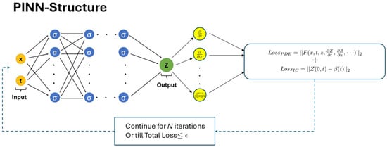
Figure 1.
Configuration of the physics-informed neural network (PINN) where ABC is not used.
To solve the Rosenau-KdV-RLW equation using an ANN method based on the PINN, we first construct a neural network architecture, as shown in Figure 1, where the ANN structure has n hidden layers and m perceptrons. Each connection between neurons (perceptrons) in adjacent layers is associated with a weight. In our case, these weights are initialized using a Glorot uniform distribution. Each neuron j in layer l (except for the input layer) has an associated bias and a set of weights connecting it to the neurons in the previous layer . The biases in our case are initialized to zeros. After the input layer, each neuron in the hidden layers and the output layer applies an activation function to the weighted sum of its inputs plus the bias. Common activation functions include ReLU (Rectified Linear Unit), Sigmoid, and Tanh. The output of neuron j in layer l is calculated as follows:
where is the activation function, are the weights, are the outputs of neurons in the previous layer, and is the bias. In this study, we employ the hyperbolic tangent function as follows:
Between the input and output layers, there are one or more hidden layers. Each hidden layer consists of neurons that take inputs from the previous layer, apply weights and biases, and pass the result through an activation function. The number of hidden layers and the number of neurons in each hidden layer are hyperparameters that are adjusted based on empirical methods.
The next process is known as feedforward propagation. During the feedforward process, the input data are passed through the network layer by layer, with each layer’s neurons performing the weighted sum of inputs and activation function calculations. The output of each layer becomes the input to the next layer until the final layer (output layer) is reached. This involves repeated application of the activation function to the weighted sum of inputs and biases. The final layer of the network is the output layer. We express the ANN solution as follows:
where n is the number of hidden layers with a width of m neurons, and
are all the weights and biases.
Here, we define our loss function as follows:
where is the training point, is the number of training points from the domain , and is the number of training points from domain .
As seen from Equations (6)–(8), only the PDE and initial conditions are included in the loss function. It should be pointed out that we add
to the loss function in order to analyze the convergence in the next section. Furthermore, the loss function does not need an artificial boundary condition for the computational domain. This is because we have used the PDE as a replacement for the boundary condition in the loss function.
Our neural network programming is executed using Python and JAX [93], Google’s open source Python library that supports in-house artificial intelligence and machine learning. Other libraries utilized include Flax [94] and Optax [95]. Flax is a high-performance neural network library and ecosystem for JAX designed for flexibility, allowing for the creation of neural networks with more fine-grained control than other libraries. Optax is a gradient processing and optimization library for JAX.
We use Optax’s Adam optimizer to update the weights and biases (parameters) based on the value of the loss function, as outlined in Algorithm 1. JAX’s automatic differentiation (autodiff) simplifies the computation of higher-order derivatives, since the functions that compute these derivatives are themselves differentiable. To evaluate our loss functions, we utilize JAX’s autodiff capabilities with the jacfwd, hessian, and vmap functions. The jacfwd function computes the Jacobian of a function, while hessian computes the Hessian. The vmap function allows us to vectorize our input, eliminating the need to create batches when handling large amounts of data.
| Algorithm 1: Adam optimizer from Optax |
 |
For the initial condition portion of our loss function, we use jacfwd and hessian below to calculate the first- and second-order derivatives of with respect to x, as seen in lines 6 and 12 of Listing 1. We then repeat this process in lines 18 and 24 to obtain the first- and second-order derivatives of with respect to x. This allows us to compute the mean squared error (MSE) of , , and , which are later used to minimize our overall loss. We employ vmap to create functions (lines 8, 14, 20, and 26) that vectorize our input data for each of the above functions. The nesting of functions is necessary for combining vectorization with the autodiff functions. This could have been made more concise if we had created a single line with nested Python Lambda functions.
It is important to note that higher-order derivatives are present in the PDE. To incorporate the loss function related only to the PDE, we create Listing 2 and use jacfwd to obtain and (lines 4 and 10). For the term and other higher-order derivatives, we chain together jacfwd and hessian calls (see lines 22, 28, and 34 in Listing 2).
| Listing 1: Loss function related to the initial conditions using jacfwd, hessian, and vmap functions. |
|
1 from jax import jacfwd, hessian, vmap 2 3 u = make_prediction(t_0, x_0) 4 5 def get_u_x(get_u, t, x): 6 u_x = jacfwd(get_u, 1)(t, x) 7 return u_x 8 u_x_vmap = vmap(get_u_x, in_axes=(None, 0, 0)) 9 u_x = u_x_vmap(make_prediction, t_0, x_0).reshape(-1,1) 10 11 def get_u_xx(get_u, t, x): 12 u_xx = hessian(get_u, 1)(t, x) 13 return u_xx 14 u_xx_vmap = vmap(get_u_xx, in_axes=(None, 0, 0)) 15 u_xx = u_xx_vmap(make_prediction, t_0, x_0).reshape(-1,1) 16 17 def get_phi_x(get_phi, x): 18 phi_x = jacfwd(get_phi, 0)(x) 19 return phi_x 20 phi_x_vmap = vmap(get_phi_x, in_axes=(None,0)) 21 phi_x = phi_x_vmap(initial_cond1, x_0).reshape(-1,1) 22 23 def get_phi_xx(get_phi, x): 24 phi_xx = hessian(get_phi, 0)(x) 25 return phi_xx 26 phi_xx_vmap = vmap(get_phi_xx, in_axes=(None,0)) 27 phi_xx = phi_xx_vmap(initial_cond1, x_0).reshape(-1,1) 28 29 mse_0_loss = MSE(u, u_0) 30 mse_0_loss_dP_x = MSE(phi_x, u_x) 31 mse_0_loss_dP_xx = MSE(phi_xx, u_xx) 32 33 Loss_Data = mse_0_loss + mse_0_loss_dP_x + mse_0_loss_dP_xx |
| Listing 2: Loss function related to the PDE using jacfwd, hessian, and vmap functions. |
|
1 from jax import jacfwd, hessian, vmap 2 3 def get_u_t(get_u, t, x): 4 u_t = jacfwd(get_u, 0)(t, x) 5 return u_t 6 u_t_vmap = vmap(get_u_t, in_axes=(None, 0, 0)) 7 u_t = u_t_vmap(make_prediction, t_c, x_c).reshape(-1,1) 8 9 def get_u_x(get_u, t, x): 10 u_x = jacfwd(get_u, 1)(t, x) 11 return u_x 12 u_x_vmap = vmap(get_u_x, in_axes=(None, 0, 0)) 13 u_x = u_x_vmap(make_prediction, t_c, x_c).reshape(-1,1) 14 15 def get_u_x_power(get_u, t, x, p): 16 u_xpower = jacfwd(get_u, 1)(t, x, p) 17 return u_xpower 18 u_x_power_vmap = vmap(get_u_x_power, in_axes=(None, 0, 0, None)) 19 u_x_power = u_x_power_vmap(make_prediction_squared, t_c, x_c, p).reshape(-1,1) 20 21 def get_u_xxx(get_u, t, x): 22 u_xxx = jacfwd(hessian(get_u, 1), 1)(t, x) 23 return u_xxx 24 u_xxx_vmap = vmap(get_u_xxx, in_axes=(None, 0, 0)) 25 u_xxx = u_xxx_vmap(make_prediction, t_c, x_c).reshape(-1,1) 26 27 def get_u_xxt(get_u, t, x): 28 u_xxt = jacfwd(hessian(get_u, 1), 0)(t, x) 29 return u_xxt 30 u_xxt_vmap = vmap(get_u_xxt, in_axes=(None, 0, 0)) 31 u_xxt = u_xxt_vmap(make_prediction, t_c, x_c).reshape(-1,1) 32 33 def get_u_xxxxt(get_u, t, x): 34 u_xxxxt = jacfwd(hessian(hessian(get_u, 1), 1), 0)(t, x) 35 return u_xxxxt 36 u_xxxxt_vmap = vmap(get_u_xxxxt, in_axes=(None, 0, 0)) 37 u_xxxxt = u_xxxxt_vmap(make_prediction, t_c, x_c).reshape(-1,1) 38 39 residual = u_t + a*u_x + b*u_x_power - c*u_xxt + d*u_xxx + u_xxxxt 40 Loss_Physics = MSE(residual) |
3. Convergence
To analyze the convergence of the ANN solution to the exact solution, we assume that , where is small, and satisfies
where and are continuous functions such that and for constants and in the closed domain . This assumption is reasonable because if there is a point such that either of the two functions is very large, then, by the continuity of that function, there is a small neighborhood around the point in which the function is also large. Since training points are randomly selected, some of the training points may fall into this small region. Thus, the function at these training points becomes very large in absolute value, which may indicate that the loss function is not satisfied. Let , where is the exact solution of Equation (1) in . One may see that satisfies
We now make a compact extension in to as
where refers to the continuity of the fourth-order derivative with respect to x and the first-order derivative to t. Here, and are any constants such that the interval is inside . Similarly, we make the corresponding compact extensions for and g as E in so that Equation (9) can be extended to
We now choose an interval such that . It can be seen that
Using the integration by parts, we have
where M is a positive constant such that . It should be pointed out that such M exists because of the continuity of and in the closed domain . Furthermore, using the Young inequality, we have
Substituting the above results into Equation (11) gives
where , with the initial condition
Solving Equation (19) gives
Hence, we integrate Equation (21) with respect to t over . This gives
Note that and are all continuous functions and is any interval such that interval is inside . We let and in Equation (22). This gives
Here, we have used the assumption of and , since we have imposed them in the loss function. This indicates that the neural network solution in is convergent to the exact solution in and the smaller is, the more accurate the ANN solution can be.
4. Numerical Experiments
To test the applicability of the present ANN method, we consider three examples for which we have exact solutions available. All models were trained using Optax’s Adam optimizer, a variant of Stochastic Gradient Descent that includes scaling adaptation through learning rate annealing. This technique systematically reduces the learning rate over time, and we set the parameters and for Algorithm 1. It should be pointed out that the default values for the variables in the Adam optimizer are typically set to and . These values are widely used in practice because they work well in many common machine learning and deep learning tasks. controls the decay rate of the moving average of the first moment (mean of gradients). A value close to 1 (like 0.9) means that the optimizer remembers gradients over a long period but still gives some weight to more recent gradients. controls the decay rate of the second moment (uncentered variance of gradients). This is important for adapting the learning rate to the variance in gradients. A value like allows the optimizer to average out the gradients’ variance over time while still adapting quickly. These values allow the optimizer to use sufficient historical information (through the exponential moving averages) while adapting the learning rate to the gradient’s scale, especially for noisy gradients. Since these defaults are consistent across popular machine learning frameworks and research papers, it is common to see them used in practice. This consistency also facilitates benchmarking and comparing results across different studies and implementations.
The computational resources used for these experiments were performed on a shared HPC cluster node using a single NVIDIA A100 GPU with 80 GB of GPU memory. The training times for each of the experiments performed took between 2 and 3.5 h. Note that the number of collocation points directly impacts the accuracy of the model. More points generally allow the network to capture the solution to the differential equations and other physics-based constraints, such as boundary and initial conditions. For complex problems, more points are necessary to ensure that the loss function adequately represents the nuances of the underlying physics. Too few points may lead to underfitting, where the network fails to learn the physics across the entire domain. On the other hand, too many collocation points can lead to overfitting, reducing the model’s ability to generalize to unseen data. Due to the complexity of the problem’s underlying physics, a large number of collocation points (40,000) were selected, based on our experience with designing physics-informed neural networks. This number was chosen to strike a balance, ensuring the network trains effectively while avoiding overburdening the hardware (GPU) and minimizing unnecessary overhead during training.
4.1. Example 1
Consider the Rosenau-KdV-RLW equation in Equation (1) with and as follows [6,63]:
subject to the initial condition
where the exact soliton solution is
In our computation, we chose a domain over the spatial interval and the time interval . We set and . From , we randomly picked 40,000 points from both the spatial and time domains, combining them into a set of coordinates as our training points. For , we randomly selected 400 training points. Figure 2 shows a snapshot of the training points.
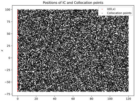
Figure 2.
Training points for Example 1.
For the ANN configuration, we designed an input layer with 2 neurons corresponding to the x and t coordinates, five hidden layers with 50 neurons each, and one output layer with 1 neuron. This architecture was selected based on multiple trials, as shown in Table 1. The model was then trained for 100,000 iterations, achieving a final loss of .

Table 1.
Neural network architecture trials.
Figure 3 shows the soliton propagation at various times . Note that we added a vertical line at the boundary in the figure. From the figure, one may see that the soliton propagates through the computational interval without reflection. In particular, we plotted the soliton at , which has passed the boundary, demonstrating that the ANN method can still predict the soliton accurately.
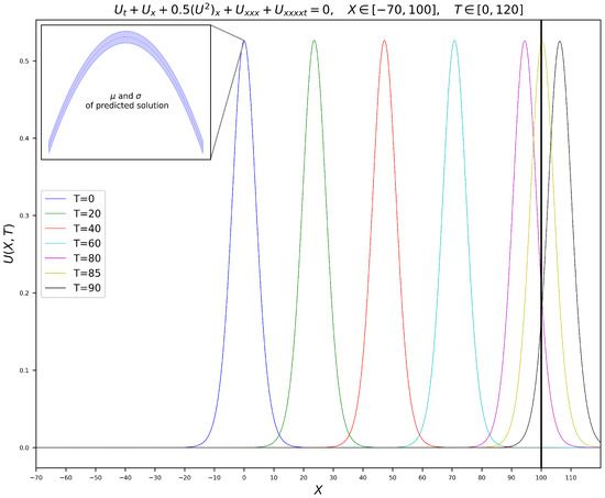
Figure 3.
Soliton propagation at various times for Example 1.
To study stability, we used three separate training runs where the only changes were the initial seed values used in the Glorot uniform distribution used to assign the initial weights of our ANN. Otherwise, all training points used were created using the same seed values to ensure reproducibility. A low standard deviation indicates that the model consistently converges to similar solutions, thus showing the stability of our model. Furthermore, note that using differing initial seed values also shows that our model is not overly sensitive to the initialization or hyperparameters, thus showing that this ANN is reliable in finding good solutions. We calculated the mean and standard deviation of the three network predictions and plotted the results. As shown in the inset of Figure 3, the standard deviation among the predictions was negligible ().
It should be pointed out out that the ANN method can still predict the soliton accurately, this is probably because predictions within the trained domain result from interpolation between known training points and the underlying physics. Outside this domain, the network has not seen the data during training, but as a universal function approximator (a feed-forward neural network with a single hidden layer that can approximate any continuous function on a compact subset of , given an appropriate activation function), it can extrapolate. If the network is well trained and the PDE solution is smooth, predictions just outside the trained region should be continuous and reasonable. However, predictions become more unreliable as the distance from the trained region increases.
Figure 4 presents a 3D plot of soliton propagation, while Figure 5 illustrates the absolute error between the ANN solution and the exact solution. The maximum absolute error between our ANN solutions and the exact solutions is , and the error in the -norm is .
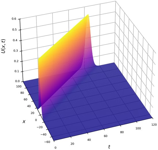
Figure 4.
3D plot of the ANN solution for Example 1.
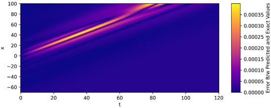
Figure 5.
Absolute error between the ANN solution and the exact solution for Example 1.
4.2. Example 2
Consider the Rosenau-KdV-RLW equation in Equation (1) with , , and as follows [6,63]:
subject to the initial condition
where the exact soliton solution is
and
In our computation, we chose a domain over the spatial interval and the time interval . We set and . From , we randomly picked points from both the spatial domain and the time domains and combined them into a set of coordinates as our training points. For , we randomly picked 400 training points. We used the same ANN configuration as that for Example 1. The model was then trained using Optax’s Adam optimizer for iterations with a final loss of .
Figure 6 illustrates the soliton propagation at various times . A vertical line has been added at the boundary . From the figure, it can be seen that the soliton propagates through the computational interval without reflection. Notably, we plotted the soliton at , which has passed the boundary, demonstrating that the ANN method can still accurately predict the soliton.
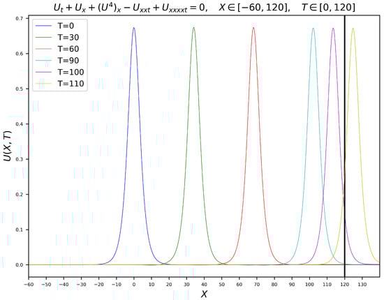
Figure 6.
Soliton propagation at various times for Example 2.
Figure 7 presents a 3D plot of soliton propagation, while Figure 8 displays the absolute error between the ANN solution and the exact solution. The maximum absolute error between our predicted solutions and the exact solutions is , and the error in the -norm is .
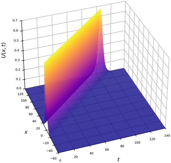
Figure 7.
3D plot of the ANN solution for Example 2.
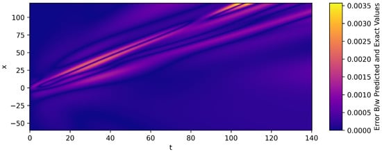
Figure 8.
Absolute error between the ANN solution and the exact solution for Example 2.
4.3. Example 3
Consider the Rosenau-KdV-RLW equation in Equation (1) with , and as follows [6]:
subject to the initial condition
where the exact soliton solution is
and
In our computation, we chose a domain over the spatial interval and the time interval . We set and . From , we randomly picked 40,000 points from both the spatial domain and the time domains and combined them into a set of coordinates as our training points. For , we randomly picked 400 training points. We used the same ANN configuration as that for Example 1. The model was then trained using Optax’s Adam optimizer for 100,000 iterations with a final loss of .
Figure 9 illustrates the soliton propagation at various times . A vertical line has been added at the boundary . From the figure, it can be seen that the soliton propagates through the computational interval without reflection. Notably, we plotted the soliton at , which has passed the boundary, demonstrating that the ANN method can still accurately predict the soliton.
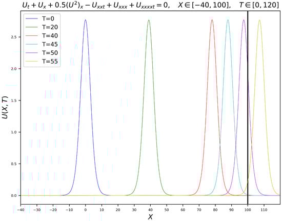
Figure 9.
Soliton propagation at various times for Example 3.
Figure 10 presents a 3D plot of soliton propagation, while Figure 11 displays the absolute error between the ANN solution and the exact solution. The maximum absolute error between our predicted solutions and the exact solutions is and the error in the -norm is .
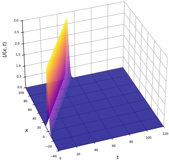
Figure 10.
3D plot of the ANN solution for Example 3.
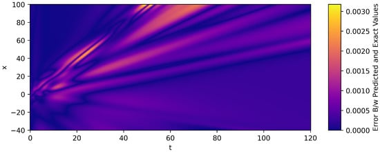
Figure 11.
Absolute error between the ANN solution and the exact solution for Example 3.
5. Conclusions
In this work, we have proposed an Artificial Neural Network (ANN) method for simulating soliton propagation based on the Rosenau-KdV-RLW equation in an unbounded domain, while the computational domain is chosen to be bounded. Unlike common numerical schemes that need ABC and PML, our ANN method can simulate the soliton propagation based on the Rosenau-KdV-RLW equation through the computational domain without using artificial boundary conditions. This is because the loss function is designed based on only the initial condition and the Rosenau-KdV-RLW equation itself and particularly for the training points on the boundary, the Rosenau-KdV-RLW equation is used as a replacement for the boundary condition in the loss function. This is the advantage of the ANN method over the common numerical schemes.
We have theoretically analyzed the convergence of the ANN solution to the exact solution. It shows that the smaller the loss function is, the more accurate the solution could be. The effectiveness of the proposed ANN method has been demonstrated through three test examples. The results indicate that the present ANN method is capable of accurately simulating soliton propagation based on the Rosenau-KdV-RLW equation in unbounded domains and/or over extended time periods.
The present study considers only 1D cases of the Rosenau-KdV-RLW equation. We will test the ANN method for the case where the exact solution of the Rosenau-KdV-RLW equation is unknown. We will further extend this research to multi-dimensional cases with soliton propagation and other wave propagations.
Author Contributions
Conceptualization, W.D. and A.B.; methodology, L.F.; computation, L.F.; visualization, L.F.; theoretical analysis, W.D.; writing—original draft preparation, L.F.; writing—review and editing, W.D. and A.B. All authors have read and agreed to the published version of the manuscript.
Funding
This research received no external funding.
Data Availability Statement
The code used in this research is publicly available on GitHub at the following repository: https://github.com/buddy-finch/Rosenau-KdV-RLW, accessed on 19 March 2025. All datasets used in this study are also available through this repository. The repository includes detailed documentation for replication and further development.
Acknowledgments
We would like to express our gratitude to Louisiana State University (LSU) and the Louisiana Optical Network Infrastructure (LONI) for providing the High Performance Computing (HPC) resources for the computations in this research.
Conflicts of Interest
The authors declare no conflicts of interest.
References
- Korteweg, D.J.; de Vries, G. XLI. On the change of form of long waves advancing in a rectangular canal, and on a new type of long stationary waves. Lond. Edinb. Dublin Philos. Mag. J. Sci. 1895, 39, 422–443. [Google Scholar] [CrossRef]
- Rosenau, P. A quasi-continuous description of a nonlinear transmission line. Phys. Scr. 1986, 34, 827. [Google Scholar] [CrossRef]
- Rosenau, P. Dynamics of dense discrete systems: High order effects. Prog. Theor. Phys. 1988, 79, 1028–1042. [Google Scholar]
- Pan, X.; Zhang, L. On the convergence of a conservative numerical scheme for the usual Rosenau-RLW equation. Appl. Math. Model. 2012, 36, 3371–3378. [Google Scholar] [CrossRef]
- Pan, X.; Zheng, K.; Zhang, L. Finite difference discretization of the Rosenau-RLW equation. Appl. Anal. 2013, 92, 2578–2589. [Google Scholar] [CrossRef]
- Wang, X.; Dai, W. A new conservative finite difference scheme for the generalized Rosenau–KdV–RLW equation. Comput. Appl. Math. 2020, 39, 237. [Google Scholar] [CrossRef]
- Guo, C.; Li, F.; Zhang, W.; Luo, Y. A conservative numerical scheme for Rosenau-RLW equation based on multiple integral finite volume method. Bound. Value Probl. 2019, 2019, 168. [Google Scholar] [CrossRef]
- Guo, C.; Wang, Y.; Luo, Y. A conservative and implicit second-order nonlinear numerical scheme for the Rosenau-KdV equation. Mathematics 2021, 9, 1183. [Google Scholar] [CrossRef]
- He, D.; Pan, K. A linearly implicit conservative difference scheme for the generalized Rosenau–Kawahara-RLW equation. Appl. Math. Comput. 2015, 271, 323–336. [Google Scholar] [CrossRef]
- Alrzqi, S.F.; Alrawajeh, F.A.; Hassan, H.N. An efficient numerical technique for investigating the generalized Rosenau–KDV–RLW equation by using the Fourier spectral method. AIMS Math. 2024, 9, 8661–8688. [Google Scholar] [CrossRef]
- Atouani, N.; Omrani, K. A new conservative high-order accurate difference scheme for the Rosenau equation. Appl. Anal. 2015, 94, 2435–2455. [Google Scholar] [CrossRef]
- Karakoc, S.B.G. A new numerical application of the generalized Rosenau-RLW equation. Sci. Iran. 2020, 27, 772–783. [Google Scholar] [CrossRef]
- Seddek, L.F.; El-Zahar, E.R.; Chung, J.D.; Shah, N.A. A novel approach to solving fractional-order Kolmogorov and Rosenau–Hyman models through the q-Homotopy analysis transform method. Mathematics 2023, 11, 1321. [Google Scholar] [CrossRef]
- Pan, X.; Zhang, L. A novel conservative numerical approximation scheme for the Rosenau-Kawahara equation. Demonstr. Math. 2023, 56, 20220204. [Google Scholar] [CrossRef]
- Jiang, C.; Cui, J.; Cai, W.; Wang, Y. A novel linearized and momentum-preserving Fourier pseudo-spectral scheme for the Rosenau-Korteweg de Vries equation. Numer. Methods Partial Differ. Equ. 2023, 39, 1558–1582. [Google Scholar] [CrossRef]
- Zhang, W.; Liu, C.; Jiang, C.; Zheng, C. Arbitrary high-order linearly implicit energy-conserving schemes for the Rosenau-type equation. Appl. Math. Lett. 2023, 138, 108530. [Google Scholar] [CrossRef]
- Zhou, Y.; Zhang, Y.; Liang, Y.; Luo, Z. A reduced-order extrapolated model based on splitting implicit finite difference scheme and proper orthogonal decomposition for the fourth-order nonlinear Rosenau equation. Appl. Numer. Math. 2021, 162, 192–200. [Google Scholar] [CrossRef]
- Wang, X.; Dai, W. A three-level linear implicit conservative scheme for the Rosenau–KdV–RLW equation. J. Comput. Appl. Math. 2018, 330, 295–306. [Google Scholar] [CrossRef]
- Abbaszadeh, M.; Zaky, M.A.; Hendy, A.S.; Dehghan, M. A two-grid spectral method to study of dynamics of dense discrete systems governed by Rosenau-Burgers’ equation. Appl. Numer. Math. 2023, 187, 262–276. [Google Scholar] [CrossRef]
- Cinar, M.; Secer, A.; Bayram, M. An application of Genocchi wavelets for solving the fractional Rosenau-Hyman equation. Alex. Eng. J. 2021, 60, 5331–5340. [Google Scholar] [CrossRef]
- Ankur; Jiwari, R.; Kumar, N. Analysis and simulation of Korteweg-de Vries-Rosenau-regularised long-wave model via Galerkin finite element method. Comput. Math. Appl. 2023, 135, 134–148. [Google Scholar] [CrossRef]
- Ghiloufi, A.; Kadri, T. Analysis of new conservative difference scheme for two-dimensional Rosenau-RLW equation. Appl. Anal. 2017, 96, 1255–1267. [Google Scholar] [CrossRef]
- Yasmin, H.; Alshehry, A.S.; Saeed, A.M.; Shah, R.; Nonlaopon, K. Application of the q-Homotopy analysis transform method to fractional-order Kolmogorov and Rosenau–Hyman models within the Atangana–Baleanu operator. Symmetry 2023, 15, 671. [Google Scholar] [CrossRef]
- Zhang, J.; Liu, Z.; Lin, F.; Jiao, J. Asymptotic analysis and error estimate for Rosenau-Burgers equation. Math. Probl. Eng. 2019, 2019, 1–8. [Google Scholar] [CrossRef]
- Wang, X.; Cheng, H.; Dai, W. Conservative and fourth-order compact difference schemes for the generalized Rosenau–Kawahara–RLW equation. Eng. Comput. 2022, 38, 1491–1514. [Google Scholar] [CrossRef]
- Shi, D.; Jia, X. Convergence analysis of the Galerkin finite element method for the fourth-order Rosenau equation. Appl. Math. Lett. 2023, 135, 108432. [Google Scholar] [CrossRef]
- Coclite, G.M.; Ruvo, L. Convergence of the Rosenau-Korteweg-de Vries Equation to the Korteweg-de Vries one. Contemp. Math. 2020, 1, 365–392. [Google Scholar] [CrossRef]
- Hu, B.; Xu, Y.; Jinsong, H. Crank-Nicolson finite difference scheme for the Rosenau-Burgers equation. Appl. Math. Comput. 2008, 204, 311–316. [Google Scholar] [CrossRef]
- Danumjaya, P.; Balaje, K. Discontinuous Galerkin finite element methods for one-dimensional Rosenau equation. J. Anal. 2022, 30, 1407–1426. [Google Scholar] [CrossRef]
- Mouktonglang, T.; Yimnet, S.; Sukantamala, N.; Wongsaijai, B. Dynamical behaviors of the solution to a periodic initial–boundary value problem of the generalized Rosenau-RLW-Burgers equation. Math. Comput. Simul. 2022, 196, 114–136. [Google Scholar] [CrossRef]
- Dangskul, S.; Suebcharoen, T. Evaluation of shallow water waves modelled by the Rosenau-Kawahara equation using pseudo-compact finite difference approach. Int. J. Comput. Math. 2022, 99, 1617–1637. [Google Scholar] [CrossRef]
- Chung, S.K.; Ha, S.N. Finite element Galerkin solutions for the Rosenau equation. Appl. Anal. 1994, 54, 39–56. [Google Scholar] [CrossRef]
- Chousurin, R.; Mouktonglang, T.; Charoensawan, P. Fourth-order conservative algorithm for nonlinear wave propagation: The Rosenau-KdV equation. Thai J. Math. 2019, 17, 789–803. [Google Scholar]
- Wang, S.; Su, X. Global existence and asymptotic behavior of solution for Rosenau equation with Stokes damped term. Math. Methods Appl. Sci. 2015, 38, 3990–4000. [Google Scholar] [CrossRef]
- Kumbinarasaiah, S.; Adel, W. Hermite wavelet method for solving nonlinear Rosenau–Hyman equation. Partial Differ. Equations Appl. Math. 2021, 4, 100062. [Google Scholar] [CrossRef]
- Zhou, D.; Mu, C. Homogeneous initial–boundary value problem of the Rosenau equation posed on a finite interval. Appl. Math. Lett. 2016, 57, 7–12. [Google Scholar] [CrossRef]
- Oruç, Ö. Integrated Chebyshev wavelets for numerical solution of nonlinear one-dimensional and two-dimensional Rosenau equations. Wave Motion 2023, 118, 103107. [Google Scholar] [CrossRef]
- Wang, Y.; Feng, G. Large-time behavior of solutions to the Rosenau equation with damped term. Math. Methods Appl. Sci. 2017, 40, 1986–2004. [Google Scholar] [CrossRef]
- Ajibola, S.O.; Oke, A.S.; Mutuku, W.N. LHAM approach to fractional order Rosenau-Hyman and Burgers’ equations. Asian Res. J. Math. 2020, 16, 1–14. [Google Scholar] [CrossRef]
- Ming, M. Long-time behavior of solution for Rosenau-Burgers equation (I). Appl. Anal. 1996, 63, 315–330. [Google Scholar] [CrossRef]
- Ming, M. Long-time behaviour of solution for Rosenau-Burgers equation (II). Appl. Anal. 1998, 68, 333–356. [Google Scholar] [CrossRef]
- Atouani, N.; Ouali, Y.; Omrani, K. Mixed finite element methods for the Rosenau equation. J. Appl. Math. Comput. 2018, 57, 393–420. [Google Scholar] [CrossRef]
- Tamang, N.; Wongsaijai, B.; Mouktonglang, T.; Poochinapan, K. Novel algorithm based on modification of Galerkin finite element method to general Rosenau-RLW equation in (2 + 1)-dimensions. Appl. Numer. Math. 2020, 148, 109–130. [Google Scholar] [CrossRef]
- Wang, X.; Dai, W.; Yan, Y. Numerical analysis of a new conservative scheme for the 2D generalized Rosenau-RLW equation. Appl. Anal. 2021, 100, 2564–2580. [Google Scholar] [CrossRef]
- Pan, X.; Wang, Y.; Zhang, L. Numerical analysis of a pseudo-compact C-N conservative scheme for the Rosenau-KdV equation coupling with the Rosenau-RLW equation. Bound. Value Probl. 2015, 2015, 65. [Google Scholar] [CrossRef]
- Labidi, S.; Rahmeni, M.; Omrani, K. Numerical approach of dispersive shallow water waves with Rosenau-KdV-RLW equation in (2 + 1)-dimensions. Discret. Contin. Dyn. Syst.-S 2023, 16, 2157–2176. [Google Scholar] [CrossRef]
- Erbay, H.A.; Erbay, S.; Erkip, A. Numerical computation of solitary wave solutions of the Rosenau equation. Wave Motion 2020, 98, 102618. [Google Scholar] [CrossRef]
- Chunk, S.K.; Pani, A.K. Numerical methods for the rosenau equation: Rosenau equation. Appl. Anal. 2001, 77, 351–369. [Google Scholar] [CrossRef]
- Özer, S. Numerical solution by quintic B-spline collocation finite element method of generalized Rosenau–Kawahara equation. Math. Sci. 2022, 16, 213–224. [Google Scholar] [CrossRef]
- Deng, W.; Wu, B. Numerical solution of Rosenau–KdV equation using Sinc collocation method. Int. J. Mod. Phys. C 2022, 33, 2250132. [Google Scholar] [CrossRef]
- Apolinar–Fernández, A.; Ramos, J.I. Numerical solution of the generalized, dissipative KdV–RLW–Rosenau equation with a compact method. Commun. Nonlinear Sci. Numer. Simul. 2018, 60, 165–183. [Google Scholar] [CrossRef]
- Verma, A.K.; Rawani, M.K. Numerical solutions of generalized Rosenau–KDV–RLW equation by using Haar wavelet collocation approach coupled with nonstandard finite difference scheme and quasilinearization. Numer. Methods Partial Differ. Equ. 2023, 39, 1085–1107. [Google Scholar] [CrossRef]
- Özer, S.; Yağmurlu, N.M. Numerical solutions of nonhomogeneous Rosenau type equations by quintic B-spline collocation method. Math. Methods Appl. Sci. 2022, 45, 5545–5558. [Google Scholar] [CrossRef]
- Ak, T.; Dhawan, S.; Karakoc, S.B.G.; Bhowmik, S.K.; Raslan, K.R. Numerical study of Rosenau-KdV equation using finite element method based on collocation approach. Math. Model. Anal. 2017, 22, 373–388. [Google Scholar] [CrossRef]
- Furioli, G.; Pulvirenti, A.; Terraneo, E.; Toscani, G. On Rosenau-type approximations to fractional diffusion equations. Commun. Math. Sci. 2015, 13, 1163–1191. [Google Scholar] [CrossRef]
- Coclite, G.M.; Ruvo, L. On the classical solutions for a Rosenau–Korteweg-deVries–Kawahara type equation. Asymptot. Anal. 2022, 129, 51–73. [Google Scholar] [CrossRef]
- Li, S.; Kravchenko, O.V.; Qu, K. On the L∞ convergence of a novel fourth-order compact and conservative difference scheme for the generalized Rosenau-KdV-RLW equation. Numer. Algorithms 2023, 94, 789–816. [Google Scholar] [CrossRef]
- Deqin Zhou, L.W.; Mu, C. On the regularity of the global attractor for a damped Rosenau equation on R. Appl. Anal. 2017, 96, 1285–1294. [Google Scholar] [CrossRef]
- Demirci, A.; Hasanoğlu, Y.; Muslu, G.M.; Özemir, C. On the Rosenau equation: Lie symmetries, periodic solutions and solitary wave dynamics. Wave Motion 2022, 109, 102848. [Google Scholar] [CrossRef]
- Wongsaijai, B.; Poochinapan, K. Optimal decay rates of the dissipative shallow water waves modeled by coupling the Rosenau-RLW equation and the Rosenau-Burgers equation with power of nonlinearity. Appl. Math. Comput. 2021, 405, 126202. [Google Scholar] [CrossRef]
- Safdari-Vaighani, A.; Larsson, E.; Heryudono, A. Radial basis function methods for the Rosenau equation and other higher order PDEs. J. Sci. Comput. 2018, 75, 1555–1580. [Google Scholar] [CrossRef]
- Muatjetjeja, B.; Adem, A.R. Rosenau-KdV equation coupling with the Rosenau-RLW equation: Conservation laws and exact solutions. Int. J. Nonlinear Sci. Numer. Simul. 2017, 18, 451–456. [Google Scholar] [CrossRef]
- Avazzadeh, Z.; Nikan, O.; Machado, J.A.T. Solitary wave solutions of the generalized Rosenau-KdV-RLW equation. Mathematics 2020, 8, 1601. [Google Scholar] [CrossRef]
- Zuo, J.M. Solitons and periodic solutions for the Rosenau–KdV and Rosenau–Kawahara equations. Appl. Math. Comput. 2009, 215, 835–840. [Google Scholar] [CrossRef]
- Prajapati, V.J.; Meher, R. Solution of time-fractional Rosenau-Hyman model using a robust homotopy approach via formable transform. Iran. J. Sci. Technol. Trans. A Sci. 2022, 46, 1431–1444. [Google Scholar] [CrossRef]
- Arı, M.; Karaman, B.; Dereli, Y. Solving the generalized Rosenau-KdV equation by the meshless kernel-based method of lines. Cumhur. Sci. J. 2022, 43, 321–326. [Google Scholar] [CrossRef]
- Muyassar Ahmat, M.A.; Jianxian Qiu, J.Q. SSP IMEX Runge-Kutta WENO scheme for generalized Rosenau-KdV-RLW equation. J. Math. Study 2022, 55, 1–21. [Google Scholar] [CrossRef]
- Kutluay, S.; Karta, M.; Uçar, Y. Strang time-splitting technique for the generalised Rosenau–RLW equation. Pramana 2021, 95, 148. [Google Scholar] [CrossRef]
- Dimitrienko, Y.I.; Li, S.; Niu, Y. Study on the dynamics of a nonlinear dispersion model in both 1D and 2D based on the fourth-order compact conservative difference scheme. Math. Comput. Simul. 2021, 182, 661–689. [Google Scholar] [CrossRef]
- Arslan, D. The comparison study of hybrid method with RDTM for solving Rosenau-Hyman equation. Appl. Math. Nonlinear Sci. 2020, 5, 267–274. [Google Scholar] [CrossRef]
- Kumbinarasaiah, S.; Mulimani, M. The Fibonacci wavelets approach for the fractional Rosenau–Hyman equations. Results Control Optim. 2023, 11, 100221. [Google Scholar] [CrossRef]
- Hasan, M.T.; Xu, C. The stability and convergence of time-stepping/spectral methods with asymptotic behaviour for the Rosenau–Burgers equation. Appl. Anal. 2020, 99, 2013–2025. [Google Scholar] [CrossRef]
- Abbaszadeh, M.; Dehghan, M. The two-grid interpolating element free Galerkin (TG-IEFG) method for solving Rosenau-regularized long wave (RRLW) equation with error analysis. Appl. Anal. 2018, 97, 1129–1153. [Google Scholar] [CrossRef]
- Sabi’u, J.; Rezazadeh, H.; Cimpoiasu, R.; Constantinescu, R. Traveling wave solutions of the generalized Rosenau–Kawahara-RLW equation via the sine–cosine method and a generalized auxiliary equation method. Int. J. Nonlinear Sci. Numer. Simul. 2022, 23, 539–551. [Google Scholar] [CrossRef]
- Özer, S. Two efficient numerical methods for solving Rosenau-KdV-RLW equation. Kuwait J. Sci. 2020, 48, 8610. [Google Scholar] [CrossRef]
- Bazeia, D.; Das, A.; Losano, L.; Santos, M.J. Traveling wave solutions of nonlinear partial differential equations. Appl. Math. Lett. 2010, 23, 681–686. [Google Scholar] [CrossRef]
- Wongsaijai, B.; Mouktonglang, T.; Sukantamala, N.; Poochinapan, K. Compact structure-preserving approach to solitary wave in shallow water modeled by the Rosenau-RLW equation. Appl. Math. Comput. 2019, 340, 84–100. [Google Scholar] [CrossRef]
- Hu, J.; Wang, Y. A high-accuracy linear conservative difference scheme for Rosenau-RLW equation. Math. Probl. Eng. 2013, 2013, 870291. [Google Scholar] [CrossRef][Green Version]
- Wongsaijai, B.; Poochinapan, K.; Disyadej, T. A compact finite difference method for solving the general Rosenau–RLW equation. IAENG Int. J. Appl. Math. 2014, 44. [Google Scholar]
- Sanchez, P.; Ebadi, Q.; Mojaver, A.; Mirzazadeh, M.; Eslami, M.; Biswas, A. Solitons and other solutions to perturbed Rosenau-KdV-RLW equation with power law nonlinearity. Acta Phys. Pol. A 2015, 127, 1577–1587. [Google Scholar] [CrossRef]
- Wongsaijai, B.; Poochinapan, K. A three-level average implicit finite difference scheme to solve equation obtained by coupling the Rosenau–KdV equation and the Rosenau–RLW equation. Appl. Math. Comput. 2014, 245, 289–304. [Google Scholar] [CrossRef]
- (Razborova) Sanchez, P.; Moraru, L.; Biswas, A. Perturbation of dispersive shallow water waves with Rosenau-KdV-RLW equation with power law nonlinearity. Rom. J. Phys. 2014, 59, 658–676. [Google Scholar]
- Ramos, J. Explicit finite difference methods for the EW and RLW equations. Appl. Math. Comput. 2006, 179, 622–638. [Google Scholar] [CrossRef]
- Raissi, M.; Perdikaris, P.; Karniadakis, G.E. Physics-informed neural networks: A deep learning framework for solving forward and inverse problems involving nonlinear partial differential equations. J. Comput. Phys. 2019, 378, 686–707. [Google Scholar] [CrossRef]
- Vadyala, S.R.; Betgeri, S.N.; Betgeri, N.P. Physics-informed neural network method for solving one-dimensional advection equation using PyTorch. Array 2022, 13, 100–110. [Google Scholar] [CrossRef]
- Cuomo, S.; Di Cola, V.S.; Giampaolo, F.; Rozza, G.; Raissi, M.; Piccialli, F. Scientific machine learning through physics–informed neural networks: Where we are and what is next. J. Sci. Comput. 2022, 92, 88. [Google Scholar] [CrossRef]
- Wen, Y.; Chaolu, T. Learning the nonlinear solitary wave solution of the Korteweg–De Vries equation with novel neural network algorithm. Entropy 2023, 25, 704. [Google Scholar] [CrossRef] [PubMed]
- Bai, Y.; Chaolu, T.; Bilige, S. Data-driven discovery of modified Kortewegde Vries equation, Kdv–Burger equation and Huxley equation by deep learning. Neural Process. Lett. 2022, 54, 1549–1563. [Google Scholar] [CrossRef]
- Jagtap, A.D.; Kharazmi, E.; Karniadakis, G.E. Conservative physics-informed neural networks on discrete domains for conservation laws: Applications to forward and inverse problems. Comput. Methods Appl. Mech. Eng. 2020, 365, 113028. [Google Scholar] [CrossRef]
- Guo, Y.; Cao, X.; Liu, B.; Gao, M. Solving partial differential equations using deep learning and physical constraints. Appl. Sci. 2020, 10, 5917. [Google Scholar] [CrossRef]
- Zhang, Z.Y.; Zhang, H.; Zhang, L.S.; Guo, L.L. Enforcing continuous symmetries in physics-informed neural network for solving forward and inverse problems of partial differential equations. J. Comput. Phys. 2023, 492, 112415. [Google Scholar] [CrossRef]
- Zhang, H.; Cai, S.J.; Li, J.Y.; Liu, Y.; Zhang, Z.Y. Enforcing generalized conditional symmetry in physics-informed neural network for solving the KdV-like equation with Robin initial/boundary conditions. Nonlinear Dyn. 2023, 111, 10381–10392. [Google Scholar] [CrossRef]
- Bradbury, J.; Frostig, R.; Hawkins, P.; Johnson, M.J.; Leary, C.; Maclaurin, D.; Necula, G.; Paszke, A.; VanderPlas, J.; Wanderman-Milne, S.; et al. JAX: Composable transformations of Python+NumPy programs. 2018. Available online: http://github.com/jax-ml/jax (accessed on 1 March 2025).
- Heek, J.; Levskaya, A.; Oliver, A.; Ritter, M.; Rondepierre, B.; Steiner, A.; Zee, M.v. Flax: A Neural Network Library and Ecosystem for JAX. 2024. Available online: http://github.com/google/flax (accessed on 1 March 2025).
- DeepMind; Babuschkin, I.; Baumli, K.; Bell, A.; Bhupatiraju, S.; Bruce, J.; Buchlovsky, P.; Budden, D.; Cai, T.; Clark, A.; et al. The DeepMind JAX Ecosystem. 2020. Available online: http://github.com/google-deepmind (accessed on 1 March 2025).


Disclaimer/Publisher’s Note: The statements, opinions and data contained in all publications are solely those of the individual author(s) and contributor(s) and not of MDPI and/or the editor(s). MDPI and/or the editor(s) disclaim responsibility for any injury to people or property resulting from any ideas, methods, instructions or products referred to in the content. |
© 2025 by the authors. Licensee MDPI, Basel, Switzerland. This article is an open access article distributed under the terms and conditions of the Creative Commons Attribution (CC BY) license (https://creativecommons.org/licenses/by/4.0/).