Abstract
The accurate, robust, and efficient prediction of transition in viscous flows is a significant challenge in computational fluid dynamics. We present a coupled high-fidelity iterative approach that leverages the FUN3D flow solver and the LASTRAC stability code to predict transition in low-disturbance environments, initiated by the linear growth of boundary-layer instability modes. Our method integrates the ability of FUN3D to compute mixed laminar–transitional–turbulent mean flows via transition-sensitized Reynolds-Averaged Navier–Stokes equations with the ability of LASTRAC to perform linear stability analysis, all within an automated framework that requires no intermediate user involvement. Unlike conventional frameworks that rely on classical stability theory or reduced-order metamodels, our approach employs parabolized stability equations to provide more accurate and reliable estimates of disturbance growth for multiple instability mechanisms, including Tollmien–Schlichting, Kelvin–Helmholtz, and crossflow modes. By accounting for the effects of mean-flow nonparallelism as well as the surface curvature, this approach lays the foundation for improved N-factor correlations for transition onset prediction in a broad class of flows. We apply this method to three distinct flow configurations: (1) flow over a zero-pressure-gradient flat plate, (2) the NLF-0416 airfoil with both natural and separation-induced transition, and (3) a 6:1 prolate spheroid, where transition is primarily driven by crossflow instability. For two-dimensional cases, a formulated intermittency distribution is used to model the transition zone between the laminar and fully turbulent flows. The results include comparisons with experimental measurements, similar numerical approaches, and transport-equation-based models, demonstrating good agreement in surface pressure coefficients, transition onset locations, and skin-friction coefficients for all three configurations. In addition to contributing a couple of new insights into boundary-layer transition in these canonical cases, this study presents a powerful tool for transition modeling in both research and design applications in aerodynamics.
Keywords:
Reynolds-averaged Navier–Stokes equations; parabolized stability equations; hydrodynamic stability analysis; transition prediction MSC:
76F06
1. Introduction
From the NASA Computational Fluid Dynamics (CFD) Vision 2030 Study [1], one of the most important fluid dynamics research areas that will remain a pacing item for the foreseeable future is the ability to accurately, robustly, and efficiently predict transition to turbulence in viscous flows. Laminar–turbulent boundary-layer transition has many applications to aerodynamic design that include unmanned aerial vehicles, natural laminar flow surfaces, and crewed re-entry vehicles [2]. Maximizing the laminar regions on aerodynamic surfaces by delaying or preventing the onset of transition substantially reduces drag, which increases the energy efficiency by reducing the fuel burn rate [3]. The energy efficiency of new and existing aircraft has to be significantly improved in order to reduce the negative impact that aviation has on the environment [4]. For high-speed flow on vehicle surfaces, transition to turbulence can result in a fivefold to eightfold increase in the skin-friction drag and heat flux. Uncertainties in transition prediction can have a critical impact on the safety, design, and performance of an aerospace vehicle, including weight, structure, and engine operability.
The common approaches to model and investigate boundary-layer transition are Direct Numerical Simulations (DNS), Reynolds-Averaged Navier–Stokes (RANS) equations, and Wall-Resolved Large-Eddy Simulations (WRLES). The use of DNS or WRLES to study transition requires substantial computational resources, especially if extended to high Reynolds numbers, where the required grid resolution is extremely fine. Moreover, these expensive simulations must have accurate initial and boundary conditions based on either wind-tunnel measurements or flight tests. RANS-based transition models that rely on various transport equations are less computationally expensive than DNS and WRLES but can be inaccurate for several reasons, including their inability to capture the process of laminar–turbulent boundary-layer transition, which involves complicated physics, including the receptivity, linear amplification, and nonlinear interactions and breakdown of instability waves. Furthermore, many RANS-based transition models are only accurate in the parameter space (or transition scenario) where they were originally calibrated, and, outside of this parameter space, i.e., very low freestream turbulence intensity values, very small Reynolds numbers, or very large Reynolds numbers, they do not provide good predictions, unless they are recalibrated or updated to fix certain discrepancies. A well-known example of this drawback is the 2009 version of the Langtry–Menter - transition model [5] that does not behave as well at freestream turbulence intensity values below 0.1% as the correlation for grows exponentially.
To improve the accuracy and robustness of RANS-based models, they can be paired with more physics-based linear stability analysis techniques through a modular approach that is conducted in this work since directly integrating stability analysis techniques into particular Navier–Stokes flow solvers can be difficult. Semiempirical correlation-based methods that rely on Linear Stability Theory (LST) are often employed to predict transition locations in various flow configurations. The method developed by Smith and Gamberoni [6] as well as van Ingen [7] is the most commonly used and cited in the literature. This method seeks to correlate the onset of transition with the location where the peak amplification factor reaches a critical value of . Here, the value of is determined by experimental measurements. A well-known problem with the method is that receptivity and nonlinear breakdown cannot be modeled accurately with just a single value of . Therefore, variable N-factor methods have been proposed by Mack [8] as well as by Crouch and Ng [9]. The Parabolized Stability Equations (PSE) [10] can also be employed to predict transition. These equations are less restrictive than LST because they do not require a parallel flow assumption. Both LST and PSE can account for the amplification of Tollmien–Schlichting (TS) waves, stationary/traveling crossflow vortices, and other types of instability mechanisms. However, the application of PSE provides a more accurate prediction of the disturbance growth characteristics by accounting for the effects of mean-flow nonparallelism as well as the surface curvature. These effects can be rather important in the context of laminar flow aircraft, as shown by Malik et al. [11].
There has been considerable past work on coupling simulation tools, primarily RANS transport-equation-based models, with various linear stability analysis methods [12,13,14,15,16,17], but they have a few shortcomings. First, the use of stability analysis includes an increased computational cost and complexity, requires a CFD user with knowledge of transition physics and hydrodynamic stability theory, and usually lacks robustness. Also, modern commercial CFD codes often rely on massive parallelization and unstructured grids, which are not compatible with the global dependence of the stability characteristics in one or more spatial directions. In some cases, less accurate surrogate models that utilize laminar flow field data are employed instead of direct calculations of the stability characteristics [18,19,20,21]. For those codes that do compute the stability characteristics directly, they are tightly coupled to specific data structures that are used within their CFD solver, which makes a number of algorithmic tasks, such as the extraction of boundary-layer profiles, difficult and costly in the context of a parallel computing framework. They also cannot be easily ported to other flow solvers. Automated initiation of PSE computations that leads to minimal initial transients is also a difficult task (refer to Kosarev et al. [22] and Halila et al. [17]), commonly resulting in the adoption of simpler approaches, such as classical LST, for predicting instability growth.
The present study implements a coupled iterative approach that uses a combination of RANS basic states computed with FUN3D, an unstructured finite-volume RANS solver [23], and local stability analysis performed with LASTRAC, a state-of-the-art LST and PSE solver [24], to model boundary-layer transition. A solver-independent module that couples FUN3D and LASTRAC automatically identifies the viscous surfaces for transition prediction, extracts wall-normal boundary-layer profiles from the CFD solution, and defines integration trajectories (typically in the form of streamlines) for stability analysis with no user involvement. This solver-independent module can be coupled to any flow solver or stability code, as outlined in Choudhari et al. [2]. We determine the locations of transition onset in the FUN3D basic states with LASTRAC stability calculations that involve computing N-factor envelopes with PSE in an iterative procedure. This approach is robust because we are taking into account the growth of several different instability waves. It also does not take long to converge the transition location (both in terms of computational time and number of iterations). Furthermore, it has the potential to leverage unique capabilities in the NASA FUN3D suite of codes, which include automated grid adaptation [25,26] and the ability to perform adjoint-based design [27,28]. A similar automated iterative transition-prediction approach that couples a structured overset-grid flow solver, i.e., OVERFLOW, and LASTRAC has been verified and validated in recent work by Venkatachari et al. [29].
The work presented here is an extension of Hildebrand et al. [30]. We apply our automated FUN3D–LASTRAC iterative approach to low-speed flow over a zero-pressure-gradient flat plate, the NLF-0416 airfoil at an angle of attack equal to 5 degrees, and the 6:1 prolate spheroid at an angle of attack equal to 24 degrees. Three different transition scenarios are investigated. Natural transition occurs for the flat-plate case, both natural and separation-bubble-induced transition happen for the NLF-0416 airfoil, and crossflow instabilities primarily cause transition away from the windward and leeward planes of symmetry on the 6:1 prolate spheroid. Comparisons are conducted between results from our approach, experimental measurements, transport-equation-based models, and results from similar numerical iterative transition-prediction approaches. This paper is structured in the following manner. Section 2 describes the Spalart–Allmaras (SA) model with and without imposed transition in FUN3D, the linear stability analysis methods in LASTRAC, and the solver-independent module. The transitional results from the flat-plate, airfoil, and spheroid cases are presented in Section 3. We conclude the paper in Section 4.
2. Methodology
The proposed methodology seeks to predict boundary-layer transition over both 2D and 3D flow configurations. Practical configurations often require unstructured mesh computations. To that end, we describe an implementation that employs the FUN3D suite of codes [23,31] to compute the RANS transitional basic states, the LASTRAC suite for stability analysis [24], and the solver-independent module written in Python 3.4.3/C++11 to convert the basic states to wall-normal boundary-layer profiles and compute the streamlines for spatially marching linear stability analysis. Our iterative FUN3D–LASTRAC approach is more computationally expensive than solely using a RANS-based transition model, e.g., the Langtry–Menter (LM) - model [5], but it provides a better physics-based representation because it captures several different types of instability modes. It is also considerably less expensive than DNS or LES. The different parts of our approach (i.e., basic state computations, stability analysis, and the solver-independent module) are discussed in the following three subsections.
2.1. FUN3D Basic States
To compute the basic states, we utilize the suite of codes known as FUN3D, which is an implicit node-centered unstructured-grid upwind-biased flow solver [23]. FUN3D has the ability to compute a laminar, transitional, or fully turbulent basic state. Several different RANS-based turbulence and transition models can be run with the NASA FUN3D CFD solver, including the SA turbulence model [32], the LM transition model [5], and Coder’s Amplification Factor Transport (AFT) transition model [14]. The inviscid fluxes are computed at edge medians with Roe’s scheme [33]. Second-order accuracy is achieved via MUSCL reconstruction with unweighted least-squares nodal gradients. The viscous fluxes are computed with Green–Gauss element-based gradients at dual faces. A point implicit procedure is used to solve the linear system of equations at each time step. Each of the FUN3D simulations are run until the residuals have reached machine zero and leveled out. For more information on the various numerical methods in FUN3D, see the current version of the manual [31].
In this work, the SA one-equation turbulence model [32] with and without imposed transition is solved for the 2D and 3D basic states of low-speed flow over a flat plate, the NLF-0416 airfoil, and the 6:1 prolate spheroid. This particular RANS model is given by the following expression
where is the turbulent eddy viscosity, , , is the molecular kinematic viscosity, , is the vorticity magnitude, d is the nearest wall distance, , , , , , and is the intermittency function. The boundary conditions are at the wall and to at the farfield. For the different transitional cases in this paper, we modify the boundary conditions in the farfield such that . This lower value helps to avoid contamination of the laminar boundary layers. Also, the constants are , , , , , , , , , and . For a more complete list of the constants, function definitions, boundary conditions, and limiters, see Ref. [32] or the NASA Turbulence Modeling Resource (https://turbmodels.larc.nasa.gov/, accessed on 20 March 2025).
The specification of transition to turbulence along a viscous boundary is possible in the FUN3D suite of codes. For the 2D basic states, an intermittency function is used that multiplies the production terms of any turbulence model equations. This intermittency function is defined as
which is taken from Dhawan and Narasimha [34]. Here, represents the location of transition onset, and corresponds to the transition length. For separation-induced transition, and following Krumbein [35]. In the case of TS waves, and from Dhawan and Narasimha [34]. Note that Re∞ is the freestream unit Reynolds number, is the displacement thickness, and is the momentum thickness.
2.2. LASTRAC Stability Analysis
In the LASTRAC stability analysis tool package [24], both LST and PSE can be run for 2D and 3D RANS basic states. The linear disturbance amplification is computed with PSE from LASTRAC [36,37] in this work. These perturbations can be assumed to be harmonic in the spanwise direction, z, and in time, t, such that
where denotes the complex conjugate, is the spanwise wavenumber, and is the angular frequency. Here, and . The variables are the streamwise, wall-normal, and spanwise coordinates, respectively, with the variables representing the velocity components in those coordinate directions. We employ PSE instead of LST in this work because it accounts for the streamwise variation in the boundary-layer thickness and shape of the disturbance field. PSE solves an approximate form of the Navier–Stokes equations for a slowly varying shape function and a complex streamwise wavenumber such that
According to linear stability analysis, transition occurs at the streamwise location where the N-factor value of any fixed-frequency/fixed-wavelength disturbance first reaches a critical value of . The N-factor is defined as
where denotes the lower-branch location where the disturbance at any given frequency and wavelength combination first becomes unstable, and the kinetic-energy norm K is
The superscript denotes the Hermitian operator. To acquire the N-factor envelope over all selected disturbances, we calculate the maximum N-factor at each streamwise station. The location of transition onset is where the N-factor envelope first reaches . In general, the value of can be specified as part of the user input. However, if we know the measured turbulent intensity , we can use the expression from Mack [8] for TS waves in 2D flows. The quantity can be obtained from experimental measurements or workshops. For more complicated 3D flows that contain both TS waves and crossflow instability, the expression is used to determine a transition front. The requirement of prescribing the value forms a limitation of the N-factor methods as described by Choudhari et al. [2]; however, that requirement simply represents the sensitivity of the transition process to the external disturbance environment.
2.3. Solver-Independent Module and Iterative Approach
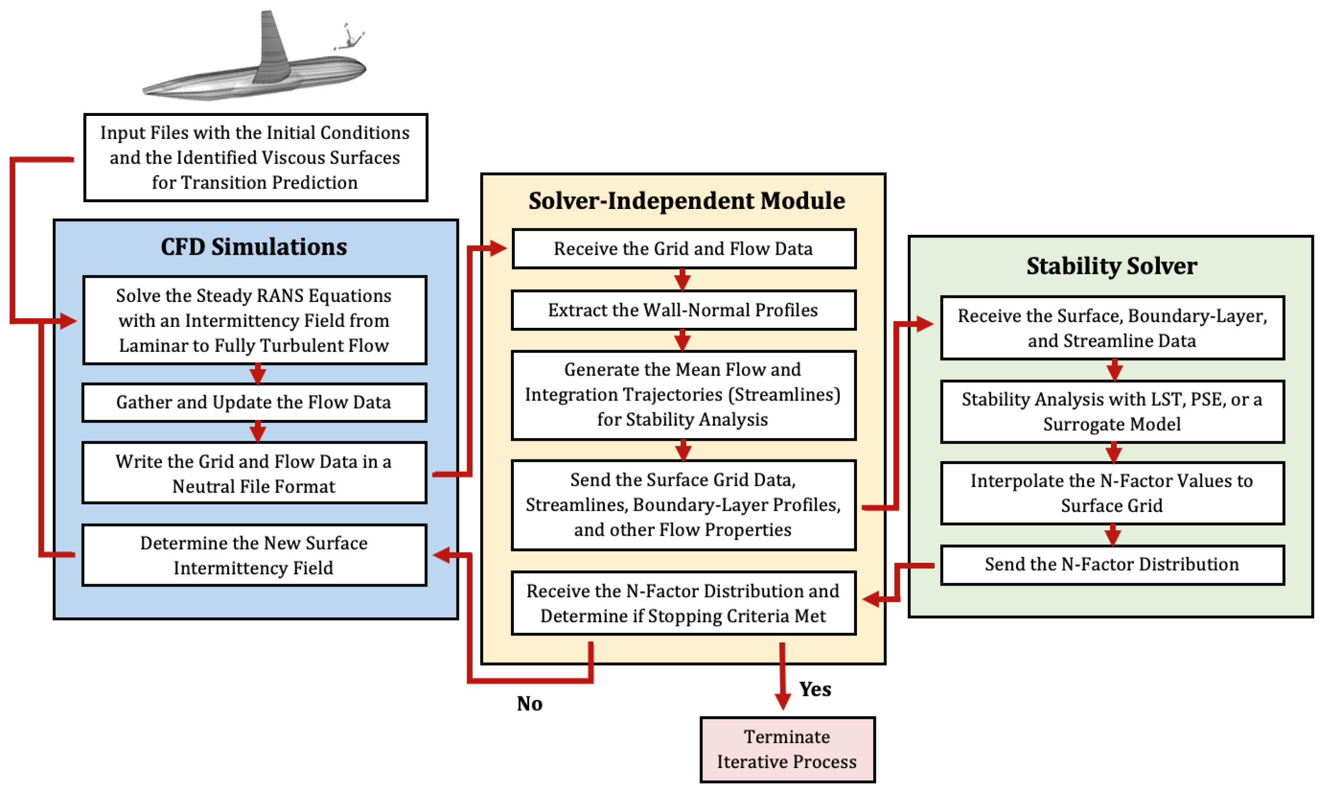
A diagram of the automated iterative coupling approach for transition prediction is displayed in Figure 1. It consists of the FUN3D v14.0.2 and LASTRAC v3.0 software packages that both can be run in parallel. The solver-independent module listed in Figure 1 is designed to couple any CFD simulation code with any stability analysis tool. Specifically, the solver-independent module in this work couples FUN3D with LASTRAC. The solver-independent module is written in Python/C++ and can also be run in parallel. It reads the grid and output solution data from the flow solvers (i.e., FUN3D and LASTRAC) in ASCII or binary format, extracts wall-normal boundary-layer profiles from the CFD solution, identifies viscous surfaces for transition prediction, forms integration trajectories or streamlines, and determines the stopping criteria. The iterative procedure in this work begins with loading the required FUN3D, LASTRAC, and Python/C++ modules. Next, a Python code generates the FUN3D input files, i.e., the name list and the job script, gathers the other required files, e.g., the computational grid and the boundary conditions, and runs the simulation in parallel. Once the FUN3D simulation has finished, the solver-independent module reads in the FUN3D solution from a binary volume file, extracts the boundary-layer profiles, identifies the viscous surfaces, and forms the integration trajectories for stability analysis. Afterward, the solver-independent module uses all this information to write a binary file of the mean flow that LASTRAC is able to read. Next, a Python code generates the LASTRAC input files and runs the stability analysis either in parallel or with multithreading. The stability analysis computations require a significant amount of memory. Once the stability analysis has finished, the N-factor values are interpolated onto the surface grid. Afterward, the solver-independent module reads in the N-factor distribution and determines the next transition location. This location of transition onset is enforced in the new FUN3D simulation as part of the next iteration.
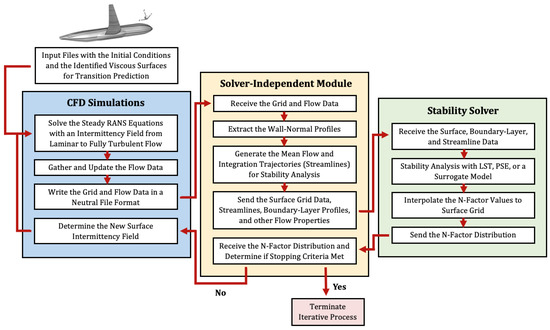
Figure 1.
Automated iterative coupling approach for CFD transition modeling using the NASA FUN3D and LASTRAC solvers that can also be substituted with any simulation or stability code based on Hildebrand et al. [30], Venkatachari et al. [29], and Choudhari et al. [2].
We determine the location of transition onset from the fixed value of and the N-factor distribution. An under-relaxation expression is used to improve the iterative convergence and is given by the following expression
where the factor is a specified value between 0.7 and 1.0, is where intersects the N-factor envelope, is the previous transition location, and is the new transition location. If the new location of transition onset, intermittency field, or 3D transition front is within a given tolerance of the same quantity for the previous iteration, our automated iterative method terminates; otherwise, it continues to iterate by setting up and running the next FUN3D simulation. If a steady RANS basic state does not fully converge to machine zero due to strong unsteadiness, nonlinearities, or a poor initial approximation of a transition location/front (usually too far downstream), then stability analysis is still applied to it, and, if the appropriate unstable mode is not found, then our automated coupled approach will shift the corresponding transition location/front upstream. On the other hand, if a transition location/front is too far upstream, producing a very small region of laminar flow, and the critical N-factor value is not reached from the spatial growth of the appropriate unstable mode, then our automated coupled approach will extrapolate the spatial growth of that unstable mode downstream into the fully turbulent region to provide a best estimate of the next transition location/front downstream.
For the computations of TS waves along streamlines, the wave angle is set to zero because the most unstable TS waves in low-speed flows are usually assumed to follow the inviscid streamline for any given disturbance frequency. In terms of stationary crossflow disturbances, a nonorthogonal coordinate is utilized at each point along the streamline, where the x coordinate is along the streamline direction and the spanwise or z coordinate is along the azimuthal grid line direction. An azimuthal wavenumber is imposed for axisymmetric bodies such as the 6:1 prolate spheroid. PSE N-factor integration is carried out for each frequency. The N-factor envelope across various disturbance frequencies as a function of the arc length along each streamline is used to uniquely determine the N-factor value at each streamline point. We linearly interpolate the N-factor values across streamlines to the entire viscous surface in order to determine transition locations based on a predetermined N-factor criterion.
3. Results
To demonstrate and evaluate our automated FUN3D–LASTRAC coupling approach, we examine three different canonical flow configurations: a zero-pressure-gradient flat plate, the NLF-0416 airfoil, and the 6:1 prolate spheroid. Collectively, these cases feature transition due to TS waves, separation bubbles, and crossflow instability. The computational predictions for these cases are evaluated via comparisons with experimental measurements as well as other computational predictions, including transport-equation-based models and results from similar iterative approaches for transition prediction.
3.1. Zero-Pressure-Gradient Flat Plate
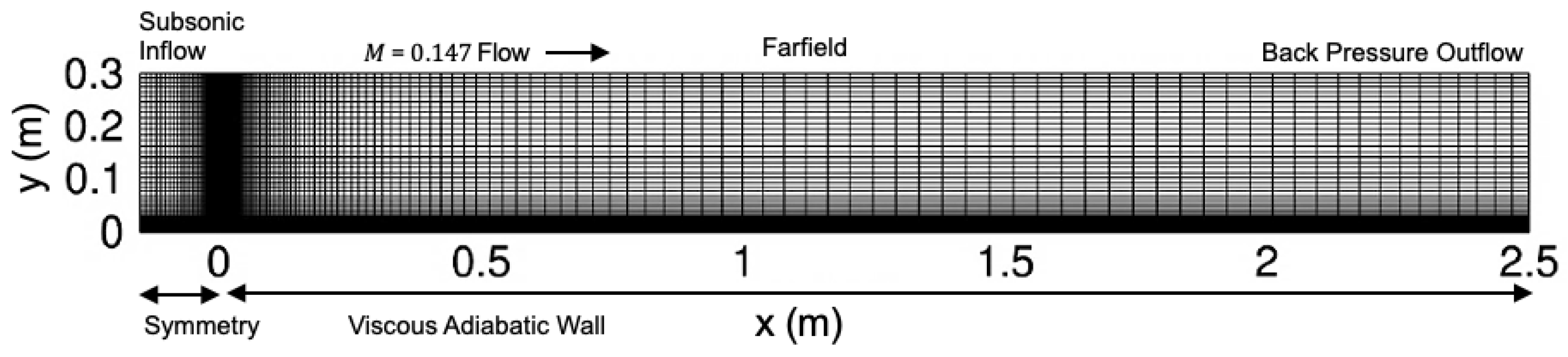
The first case we consider is low-speed flow over a two-dimensional zero-pressure-gradient flat plate with a sharp leading edge. This flat plate starts at m and extends to m. We select the flow conditions to match those from experiments by Schubauer and Skramstad [38]. The freestream density, velocity, and temperature are kg/m3, m/s, and K, respectively. This yields a freestream unit Reynolds number of m) and Mach number of . We assume a perfect gas such that , where J/K/kg is the specific gas constant for air. Here, is the constant ratio of specific heats. The Prandtl number is set to a constant value of . To compute the dynamic viscosity , we use Sutherland’s law with kg/(ms) and K. A freestream turbulence intensity of is used for this case. The left edge of the computational domain at m is a subsonic inflow, and the right edge is a back-pressure outflow. Furthermore, the flat plate has adiabatic and no-slip boundary conditions, and the small portion before the flat plate is set to a wall-normal-symmetry boundary condition. A farfield boundary condition is used at the top edge of the domain at m.
We use a computational grid with 961 and 513 points in the streamwise and wall-normal directions, respectively. The 961 points also include the 257 points upstream of the leading edge of the flat plate. We place the first grid point above the flat plate at a distance of m, which satisfies regardless of the boundary-layer state, and the wall-normal grid spacing increases gradually from there to the freestream. This computational grid is designed to have more than 150 points within the boundary layer. Furthermore, the streamwise grid spacing is the smallest near the leading edge of the flat plate at m. This exact computational grid is depicted as level 6 herein, and others in the family were used in previous work by Venkatachari et al. [39]. For grids in this family, the resolution doubles between consecutive even or odd levels. Grid level 7 has 1441 and 769 points in the streamwise and wall-normal directions, respectively, while grid level 8 has 1921 and 1025 points. Figure 2 displays grid level 1 in this family and the corresponding boundary conditions.

Figure 2.
Grid level 1 and the boundary conditions for the zero-pressure-gradient flat plate.
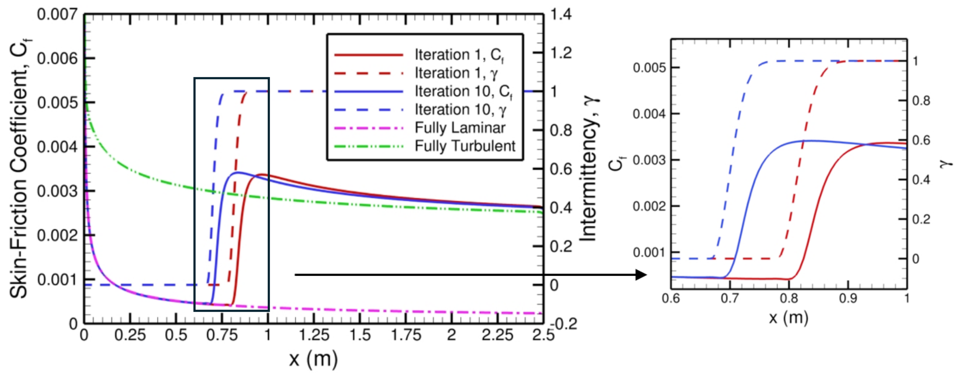
Figure 3 displays the streamwise distributions of the skin-friction coefficient and the intermittency along the plate for iterations 1 and 10 of the automated coupling approach with FUN3D and LASTRAC pertaining to grid level 6. There is a significant difference between the results from iterations 1 and 10 after transition occurs, but, upstream in the laminar portion, the solutions are the exact same. Moreover, the intermittency varies smoothly from 0 to 1 in the region of transition as the skin-friction coefficient also rises from approximately to . A closeup view of both the skin-friction coefficient and the intermittency near transition to turbulence are shown in Figure 3 on the right. As indicated in Figure 3, the intermittency function helps the flow to shift from laminar to fully turbulent over a finite streamwise extent (instead of happening very abruptly) to better match the physics and the experiments. Although not shown, it also improves the iterative convergence of the automated FUN3D–LASTRAC transition-prediction method.
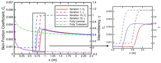
Figure 3.
The streamwise distributions of the skin-friction coefficient and the intermittency are shown for the flat-plate case from the automated FUN3D–LASTRAC method computed on grid level 6. Also, the fully laminar and turbulent solutions in terms of the skin friction are shown.
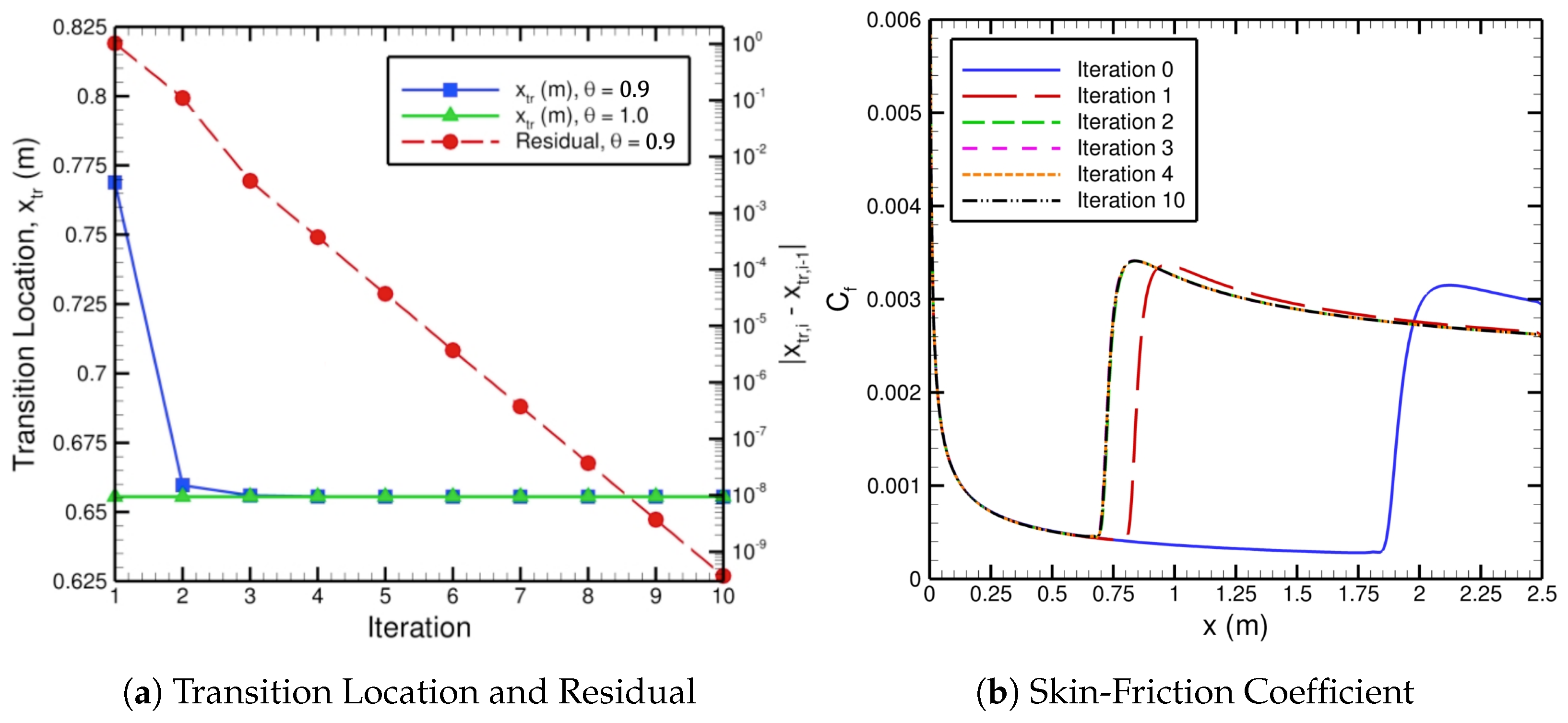
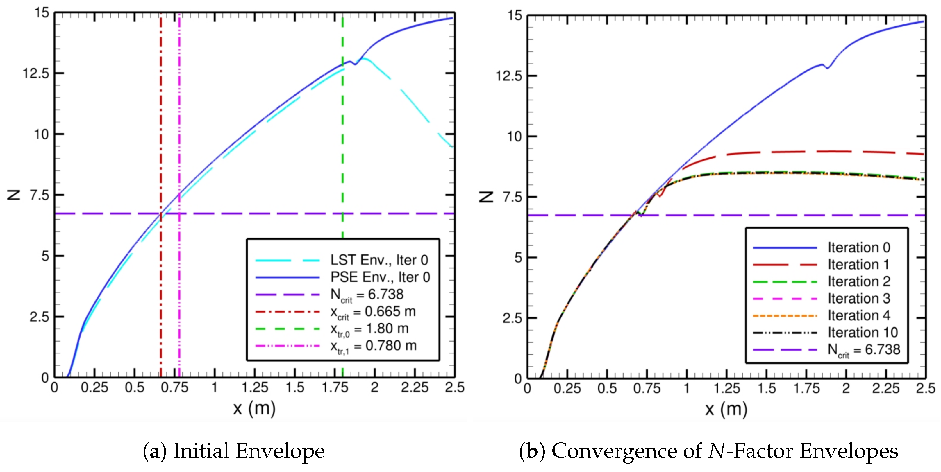
The iterative convergence of the imposed transition location with the corresponding residual and the skin-friction coefficient are displayed in Figure 4. For the initial basic state, i.e., the zeroth iteration, we imposed transition far downstream at m. The skin-friction distribution from the initial basic state is shown in Figure 4b. Once the initial FUN3D basic state has been obtained, it is converted by the solver-independent module to a format that LASTRAC is able to read. That mean flow file is used to determine the N-factor envelope based on PSE computations. The N-factor envelope of the initial basic state is depicted in Figure 5, along with the N-factor envelopes pertaining to iterations 1 through 10. The value of in Figure 5 comes from the expression via Mack [8] for TS waves in 2D flows with . Note that Mack’s correlation of is based on LST results, but, since nonparallel effects for the flat plate are rather small, the same expression may be used for the PSE as well. The location where crosses the N-factor envelope yields , which, in turn, is used to determine the next transition location, , with Equation (7) using and an appropriate under-relaxation factor. This results in the values of m and m in Figure 5 with m and for iteration 0. The new transition location, m, is prescribed in the next FUN3D basic-state computation pertaining to iteration 1. As the iteration number increases from 0 to 10, the N-factor envelopes converge in Figure 5b, and the skin-friction distributions converge in Figure 4b. The resulting change in the location of transition onset from each iteration decreases exponentially, or in a straight line on a logarithmic scale, to machine zero according to Figure 4a. Moreover, if the under-relaxation factor is set to unity (i.e., zero under-relaxation), then after just one iteration the location of transition onset converges for this flat-plate case. This means the flow does not have significant viscous–inviscid interactions and is not overly sensitive to changes in the location of transition onset. For cases with stronger viscous–inviscid interactions, under-relaxation is necessary to achieve robust convergence, especially during the early iterations, but can be increased afterwards to reduce the number of overall iterations. Similar iterative convergence of the automated FUN3D–LASTRAC method is obtained for different initially imposed transition locations of the initial basic state from m to m. If the imposed transition location is considerably upstream of the final converged transition location, then extrapolation is used to predict the next imposed transition location.
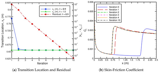
Figure 4.
Convergence of the imposed transition location with the corresponding residual and the skin-friction coefficient from the automated FUN3D–LASTRAC transition-prediction method for the zero-pressure-gradient flat plate.
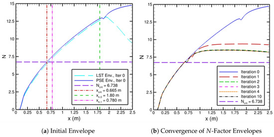
Figure 5.
N-factor envelopes computed with LST and PSE using LASTRAC and the FUN3D basic states in Figure 4b for the zero-pressure-gradient flat plate corresponding to iterations of the automated FUN3D–LASTRAC transition-prediction method.
After showing iterative convergence of the automated FUN3D–LASTRAC transition-prediction method for the zero-pressure-gradient flat plate, we focus on grid convergence for the same case. Figure 6 shows the grid convergence of the drag coefficient, transition location, and skin-friction coefficient for this flat-plate case across levels 4 through 9. The level 4 grid has 123,616 points, and the level 9 grid has 4,428,097 points, where the resolution doubles along each spatial direction every other grid level. In Figure 6a, both the drag coefficient and transition location plateau for levels 8 and 9 as the grid spacing parameter approaches zero. The skin-friction distribution also converges as the resolution increases (or the grid spacing decreases) in Figure 6b. Hence, our automated FUN3D–LASTRAC transition-prediction method converges with respect to both the iteration number and grid resolution.
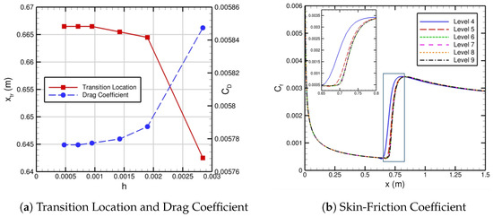
Figure 6.
Grid convergence of the imposed transition location, the drag coefficient, and the skin-friction coefficient from the automated FUN3D–LASTRAC transition-prediction method for the zero-pressure-gradient flat plate.
To validate our automated FUN3D–LASTRAC transition-prediction method, we compare the skin-friction distributions between our method, the OVERFLOW–LASTRAC method [29], the SST2003-LM2009 model [5], and the SA1994-AFT2014 model [14] in Figure 7. The experimentally observed transition zone [38] is also included as part of Figure 7 to validate our method. All the different computational skin-friction distributions begin to quickly rise in the experimentally observed transition zone [38], which indicates good agreement between the computations and experiments. The relative agreement between the skin-friction distributions computed with the FUN3D–LASTRAC and OVERFLOW–LASTRAC methods indicates that transition occurs at the exact same value of (the laminar and turbulent skin-friction coefficients also match); the only deviation is limited to the intermittent region between laminar and fully turbulent flow because the coupling methods use different intermittency functions. There is also relatively good agreement between the RANS-based transition models (i.e., SST2003-LM2009 and SA1994-AFT2014) and the automated FUN3D–LASTRAC transition-prediction method in terms of the skin-friction coefficient and the location of transition onset. These successful comparisons provide verification and validation of the FUN3D–LASTRAC approach for modeling transition for this 2D zero-pressure-gradient flat-plate case.
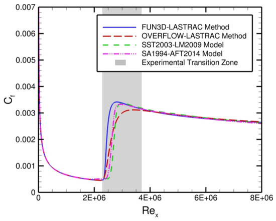
Figure 7.
Comparisons of the results from our automated FUN3D–LASTRAC transition-prediction method, the automated OVERFLOW–LASTRAC method [29], the SST2003-LM2009 model, the SA1994-AFT2014 model, and the experimental transition zone from Schubauer and Skramstad [38]. The computational results are in terms of the skin-friction coefficient, and the steep rise of that quantity means the flow is undergoing transition to turbulence.
3.2. NLF-0416 Airfoil
To help validate the automated FUN3D–LASTRAC iterative method for strong viscous–inviscid interaction and transition due to a separation bubble, we consider the NLF-0416 airfoil that is a natural-laminar-flow configuration developed at the NASA Langley Research Center by Somers [40]. This particular airfoil is designed to achieve a large value of the maximum lift coefficient and a low value of the cruise drag coefficient. An angle of attack equal to 5 degrees is considered, which leads to natural boundary-layer transition in a fully attached boundary layer over the upper surface and separation-bubble-induced transition across the lower surface. A moderate Reynolds number based on the chord length is prescribed, , and the freestream Mach number is . The freestream density, velocity, and temperature are kg/m3, m/s, and K, respectively. A freestream turbulence intensity of is used based on the benchmark problem from the 1st AIAA Transition Modeling Workshop (https://transitionmodeling.larc.nasa.gov/workshop_i/, accessed on 20 March 2025). The farfield boundaries are placed 1000 chord lengths away from the airfoil surface. Freestream boundary conditions are enforced at the left, right, top, and bottom edges of the computational domain. Adiabatic and no-slip boundary conditions are employed at the airfoil surface. This case is significantly more challenging than the flat plate because multiple applications of stability analysis for the basic states are required to capture the strong influence of the recirculation bubble on transition due to an interaction that occurs between the separation-reattachment characteristics and the location of transition onset.
We use a C-type mesh generated with conformal mapping for the NLF-0416 airfoil. The coarser levels of this mesh are based on the grids provided by the 1st AIAA Transition Modeling Workshop. Here, the level 6 grid has 2113 and 289 points along the chordwise and wall-normal directions, respectively. There are 289 points in the wake cut of the grid. It has a near-wall spacing of based on the chord length that yields a nondimensional wall spacing of approximately based on turbulent flat-plate estimates at the quarter-chord location. Furthermore, this exact computational grid (level 6) and others in the family were used in the previous work by Venkatachari et al. [39]. For grids in this family, the resolution doubles with every other level. Grid level 8 has 4225 and 577 points in the chordwise and wall-normal directions, respectively. Figure 8a displays grid level 6 in this family and the corresponding boundary conditions. There is a clustering of grid points near the airfoil surface and in the wake region.

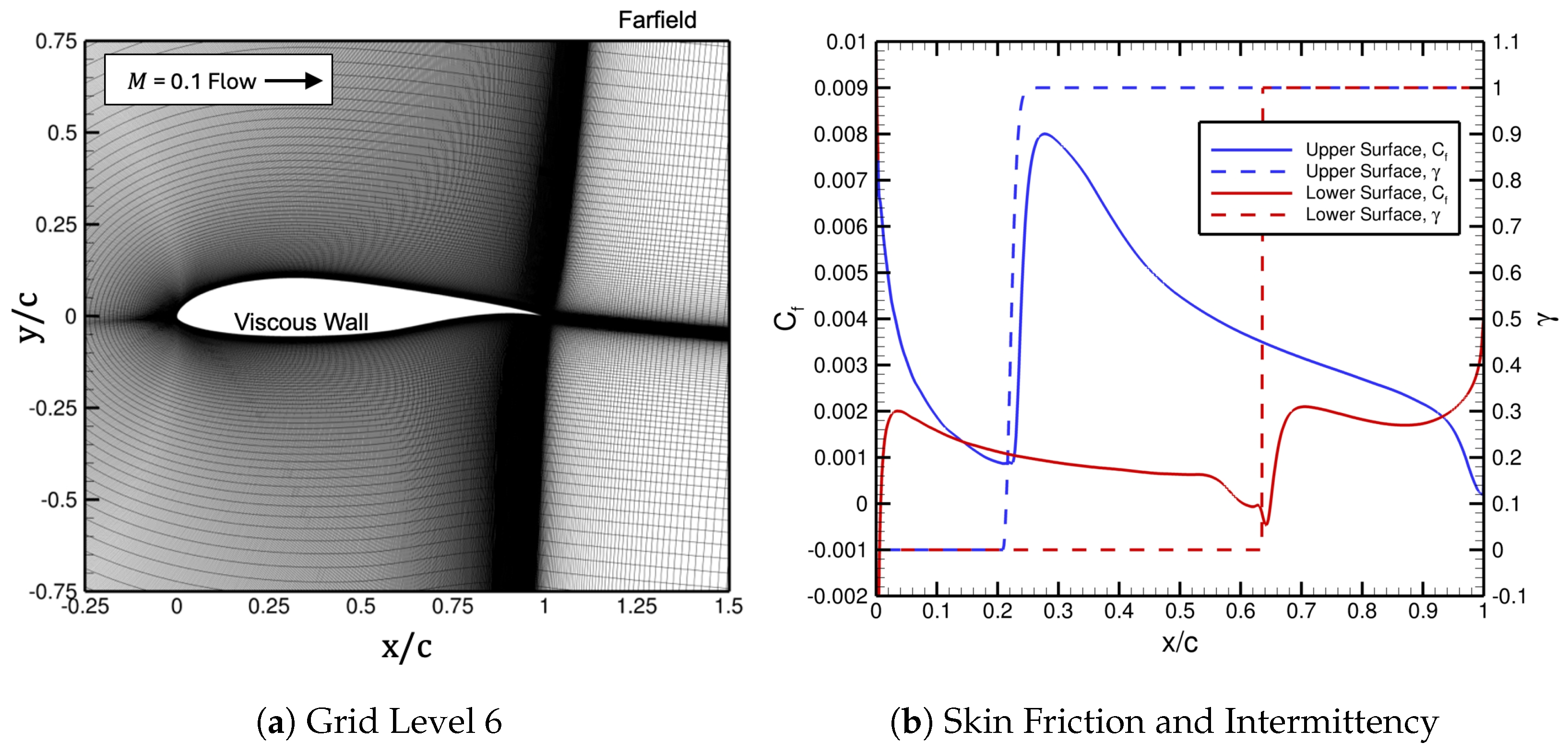
Figure 8.
Grid level 6 and the boundary conditions for the NLF-0416 airfoil. The distributions of the skin-friction coefficient and the intermittency are shown for the final iteration of the automated FUN3D–LASTRAC transition-prediction method.
The streamwise distribution of the skin-friction coefficient and the intermittency along the upper and lower surfaces of the NLF-04146 airfoil for the final iteration of the automated FUN3D–LASTRAC method computed on grid level 6 are shown in Figure 8b. The intermittency increases smoothly from 0 to 1 in the regions of boundary-layer transition occurring on the upper and lower surfaces of the NLF-0416 airfoil, while the skin friction also rises sharply in these regions. For the lower airfoil surface, there is negative skin friction within a separation bubble that causes transition, while the boundary layer on the upper airfoil surface undergoes a natural transition.
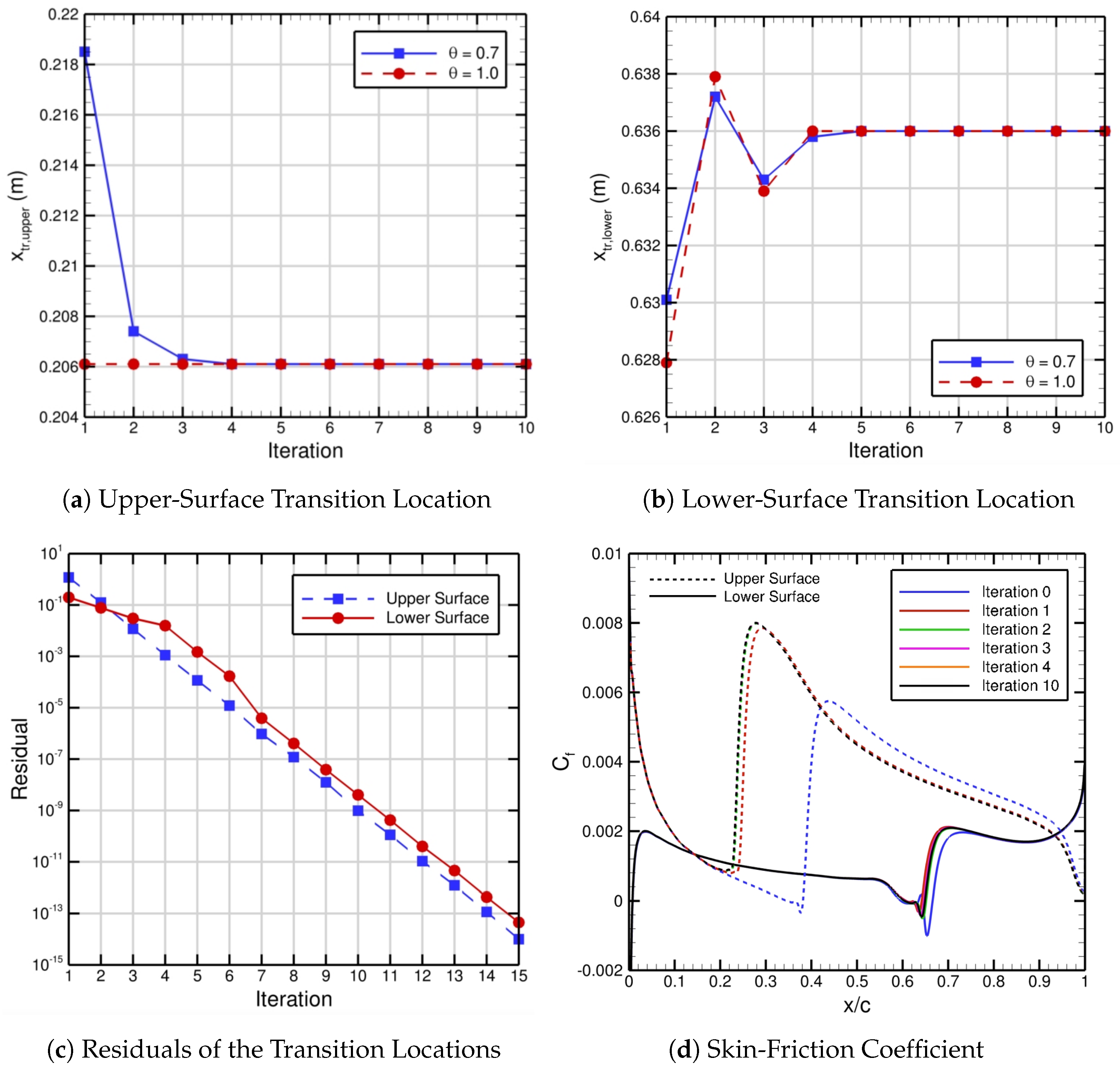
Figure 9 depicts the iterative convergence of the imposed transition locations with the associated residuals and the skin-friction distributions. For the initial basic state, i.e., the zeroth iteration, we imposed transitions at and . Note that this choice is arbitrary, and, if we imposed transition further upstream or downstream on either the upper or lower surfaces for the zeroth iteration, the final converged transition locations would be the same. The skin friction of the initial basic state is shown in Figure 9d. After the initial FUN3D basic state has been obtained, we perform the same iterative procedure conducted for the zero-pressure-gradient flat-plate case and outlined in Figure 1. Both transition locations on the upper and lower surfaces of the NLF-0416 airfoil converge in Figure 9, with values of and . In this case, we consider the flow to be converged at iteration 5 because the associated change in the locations of transition onset for the upper and lower surfaces after iteration 5 is less than m, but we also show convergence to machine zero (i.e., m) or to iteration 15 in Figure 9c. Also, the skin friction in Figure 9d is essentially identical for iterations 4 through 10. The lower under-relaxation factor of 0.7 does not have a significant benefit in this particular case, but, for initially imposed transition locations far away from their converged values and for more complex flow configurations, it helps the automated FUN3D–LASTRAC iterative method to smoothly approach the final solution. The upper-surface transition location converges similarly to the flat-plate case, but the lower-surface transition location has oscillatory convergence because of the strong influence of the separation bubble on transition to turbulence. In other words, for the lower airfoil surface, there is an interaction that occurs between the separation-reattachment characteristics and the location of transition onset. This causes the imposed transition location for the lower surface to be upstream and downstream of the final converged transition location at different iterations of the automated FUN3D–LASTRAC process.
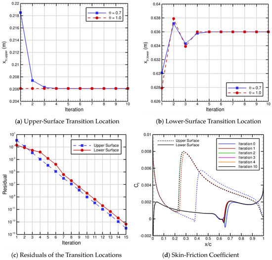
Figure 9.
Convergence of the imposed transition locations with the corresponding residuals and the skin-friction distributions from the automated FUN3D–LASTRAC transition-prediction method for the NLF-0416 airfoil.
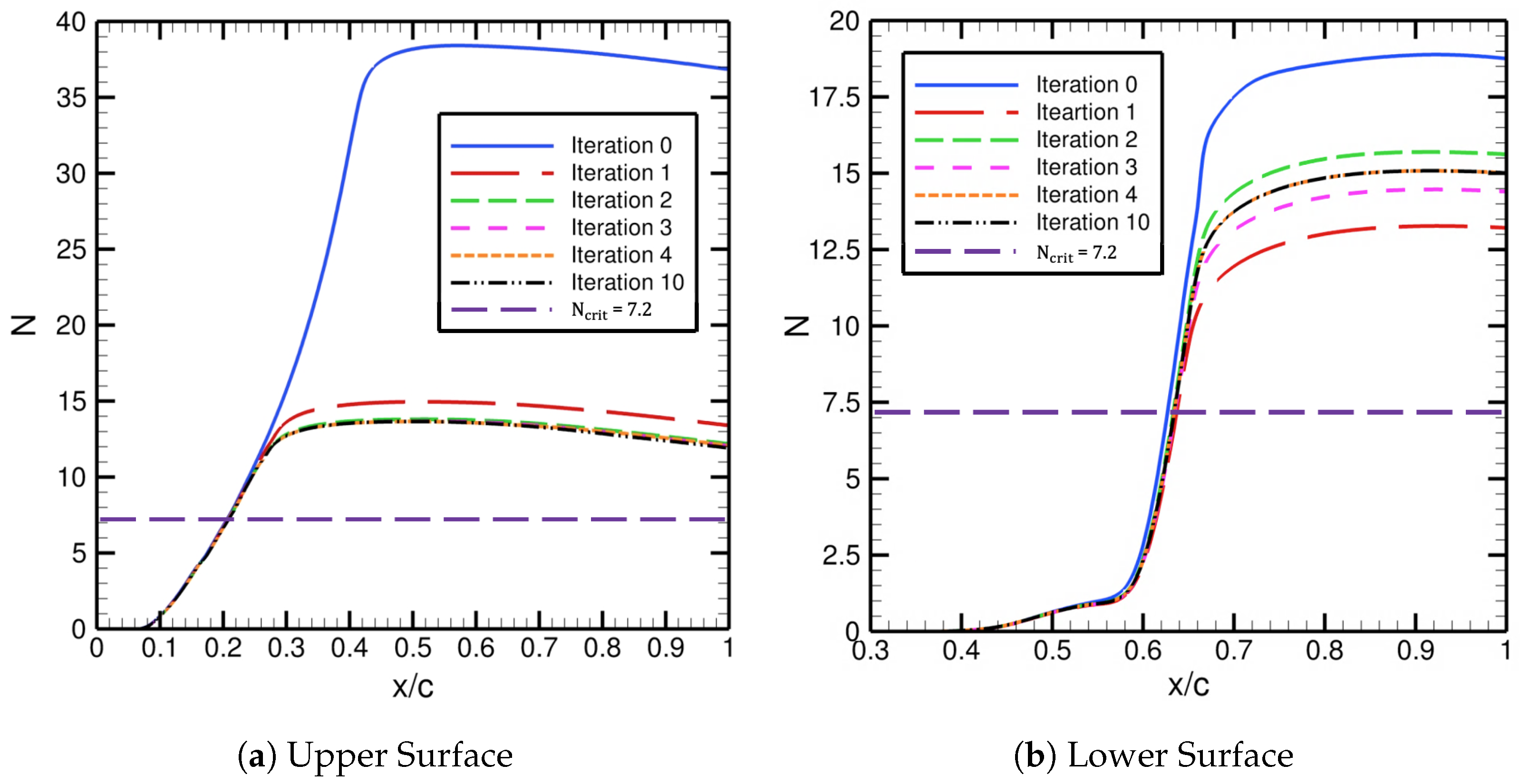
Figure 10 shows the iterative convergence of the N-factor envelopes that are computed with PSE using LASTRAC for iterations 0, 1, 3, 4, and 10. Since the value of is 0.15%, we obtain . Again, this expression from Mack [8] is based on flat-plate computations with LST (i.e., TS growth in attached boundary layers). Thus, it applies for natural transition along the upper surface, but, for the lower surface, its use for separation bubbles is somewhat arbitrary. It will be demonstrated that values based on Mack’s correlation lead to reasonable flow behavior and yield a good match with the limited available experimental measurements for this case. For the upper airfoil surface, the N-factor envelopes decrease from a maximum value of approximately 38 to 15 until convergence by about iteration 5. Moreover, for the lower airfoil surface, the maximum values of the N-factor envelopes oscillate around the final converged maximum value of 15 by iteration 4. This reaffirms the interaction that occurs between the separation-reattachment characteristics and the location of transition onset on the lower surface. Regardless of the visible influence of the separation bubble on the lower-surface transition location, the automated FUN3D–LASTRAC transition-prediction method iteratively converges quickly by iteration 4 in terms of both the skin-friction coefficient and the location of transition onset.
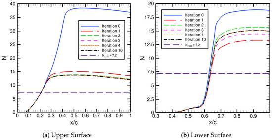
Figure 10.
Convergence of the N-factor envelopes computed with PSE from the automated FUN3D–LASTRAC transition-prediction method for the upper and lower surfaces of the NLF-0416 airfoil.
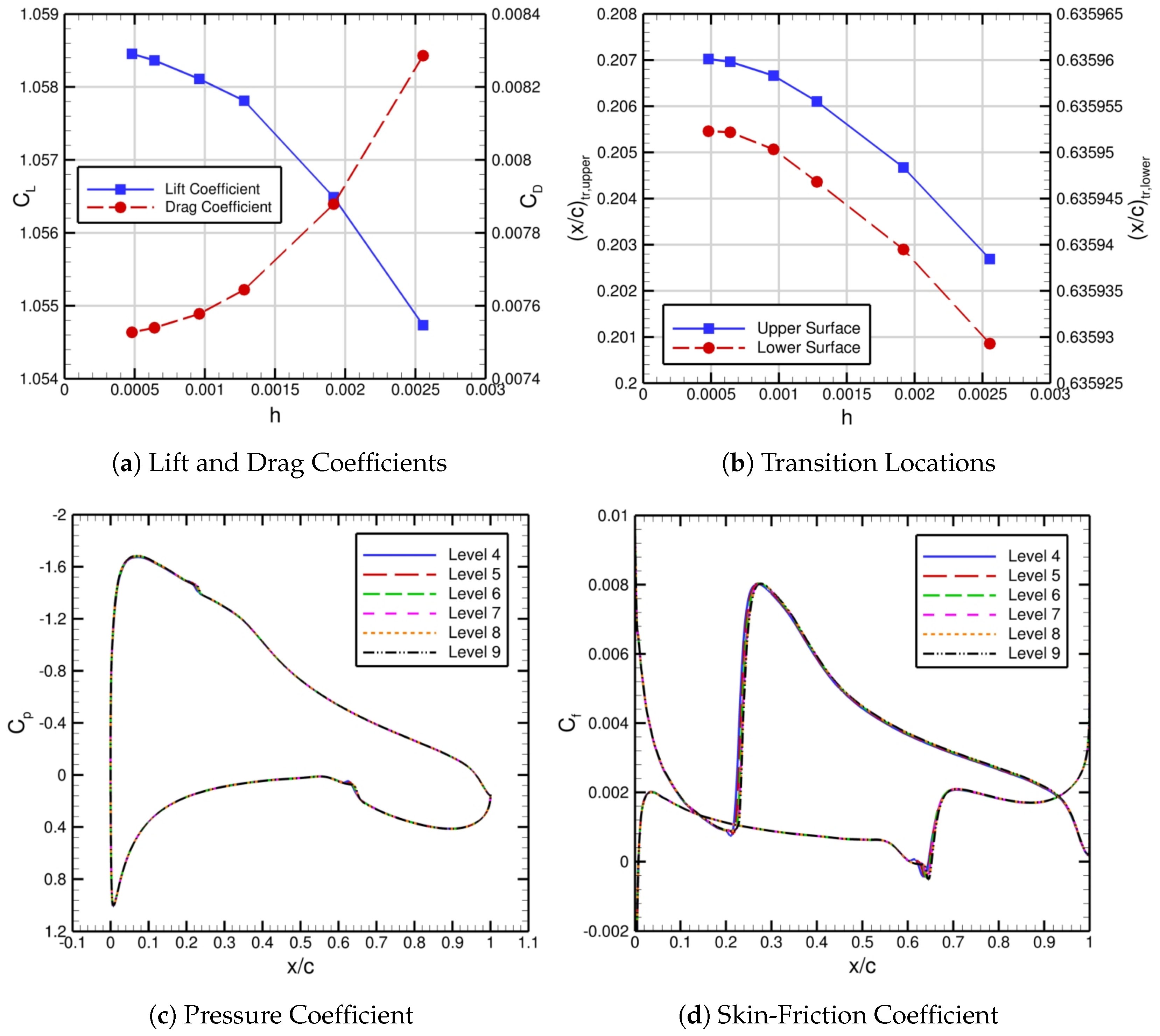
Similar to the flat-plate case, after demonstrating iterative convergence of the automated FUN3D–LASTRAC transition-prediction method for the NLF-0416 airfoil, we focus on showing grid convergence for the case. Figure 11 shows the grid convergence of the lift and drag coefficients, transition locations, and the skin-friction coefficient for the NLF-0416 airfoil via levels 4 through 9. The level 4 grid has 153,265 points, and the level 9 grid has 4,331,777 points. In Figure 11a, the lift and drag coefficients are converging as the grid spacing parameter approaches zero. Both the upper and lower transition locations in Figure 11b also converge with respect to grid resolution. Furthermore, the skin-friction distribution in Figure 11d is also grid-converged by level 9.
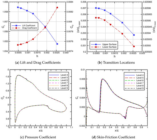
Figure 11.
Grid convergence of the lift and drag coefficients, the imposed transition locations, the pressure coefficient distributions, and the skin-friction coefficient distributions from the automated FUN3D–LASTRAC transition-prediction method for the NLF-0416 airfoil.
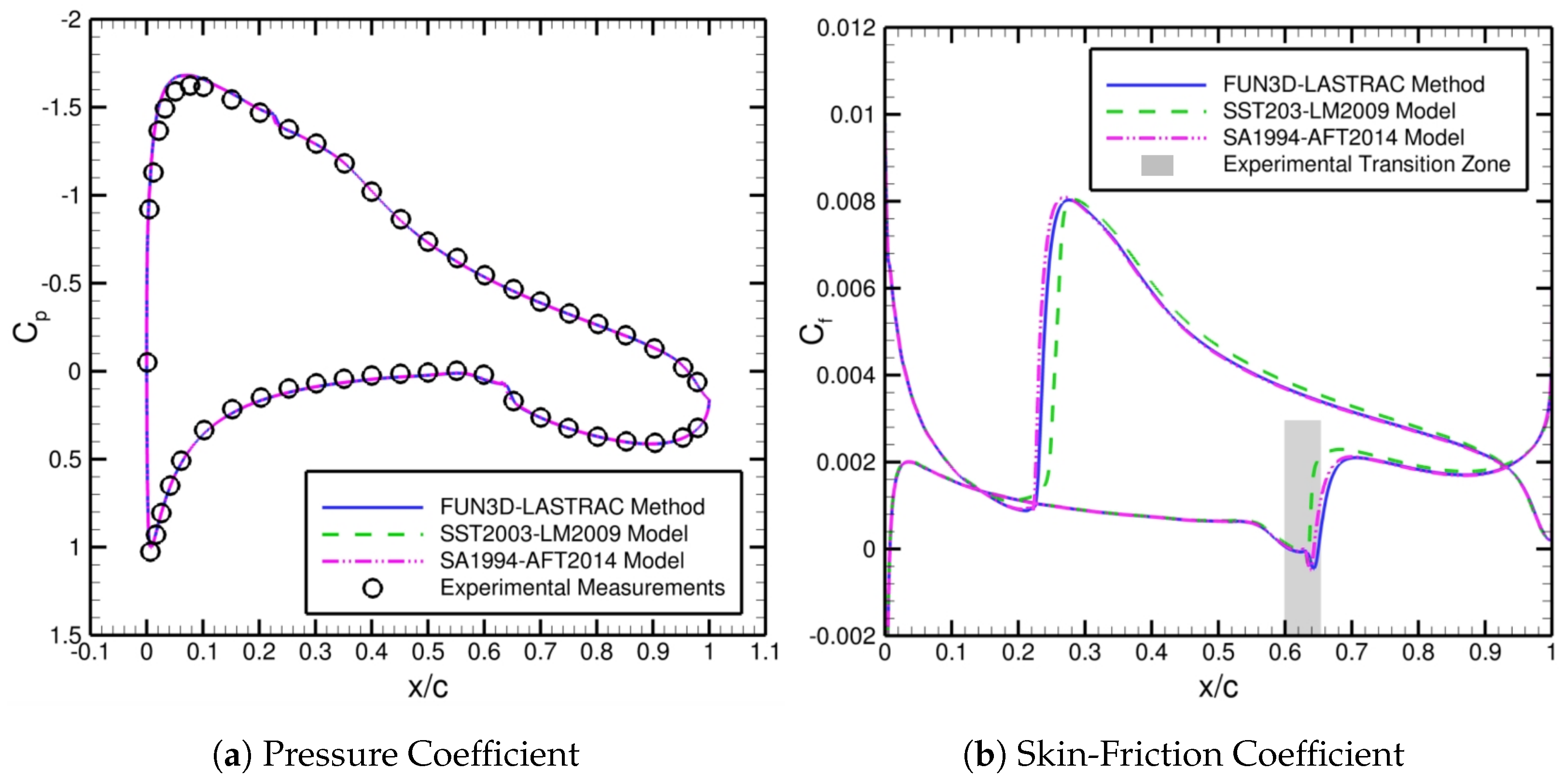
To validate our automated FUN3D–LASTRAC transition-prediction method, we compare the pressure and skin-friction coefficients between our method, the SST2003-LM2009 model [5], the SA1994-AFT2014 model [14], and experimental measurements [40] in Figure 12. There is excellent agreement between the computational and experimental results in terms of the pressure coefficient in Figure 12a. All the different computational skin-friction distributions begin to quickly rise in the experimentally observed transition zone [40] for the lower airfoil surface, which indicates good agreement between the computations and experiments in Figure 12b. Note that there are no measurements of the experimental transition zone on the upper surface. There is also good agreement between the different computational predictions (i.e., our automated FUN3D–LASTRAC transition-prediction method and two RANS-based transition models) of the skin-friction distributions and transition locations.
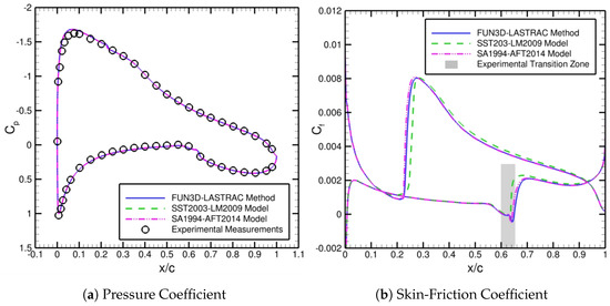
Figure 12.
Comparisons of the pressure and skin-friction coefficients from our automated FUN3D–LASTRAC transition-prediction method, the SST2003-LM2009 model, and the SA1994-AFT2014 model. The experimental measurements of the pressure coefficient and the experimental transition zone from Somers [40] are shown as well.
3.3. The 6:1 Prolate Spheroid
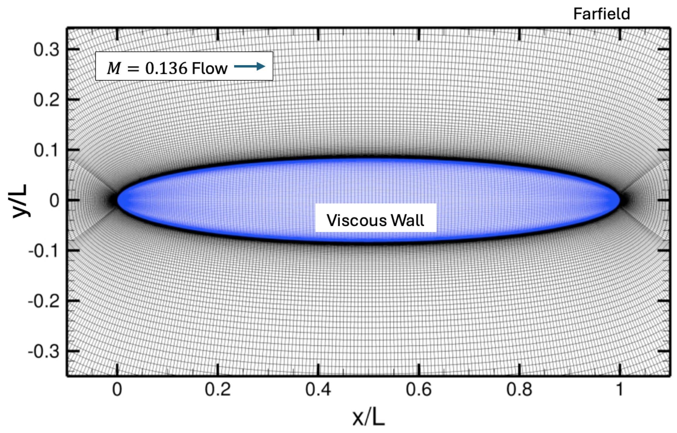
The last case we consider to validate our automated FUN3D–LASTRAC transition-prediction method is the 6:1 prolate spheroid. This geometry was experimentally investigated by Kreplin et al. [41]. Stability analysis for the 6:1 prolate spheroid has been performed by Spall and Malik [42], Stock [43], and Krimmelbein et al. [44]. The spheroid is representative of a simplified fuselage of a commercial aircraft. This flow configuration is a part of both the AIAA Transition Modeling Workshop and the AVT-313 Incompressible Flow Transition Comparison Workshop (http://web.tecnico.ulisboa.pt/ist12278/Workshop_AVT_313_2D_cases/Workshop_AVT_313_2D_cases.htm, accessed on 20 March 2025). We consider an angle of attack equal to 24 degrees. The freestream Mach number, temperature, and Reynolds number based on the spheroid length are 0.136, 300 K, and , respectively. A freestream turbulence intensity of is used for this case. The spheroid length is equal to 2.4 m. Transition can occur via TS waves and crossflow instability. Farfield boundary conditions are employed at the domain edges approximately 100 spheroid lengths away from the viscous surface, except for a symmetry boundary condition that is employed on the plane at . Adiabatic and no-slip boundary conditions are enforced on the spheroid surface. We have run a few representative cases using our coupled iterative approach for the 6:1 prolate spheroid with the entire geometry and flow field, i.e., no symmetry assumption, and the results are identical to simplified cases with the symmetry assumption.
Figure 13 depicts the lowest-resolution (i.e., level 3) computational grid on the spheroid surface and within the plane for better visibility. We use a multiblock structured grid to avoid singularities along the major axis of the spheroid model near the nose and the aft end of the geometry. Totals of 65, 65, and 257 points are used in the streamwise, azimuthal, and wall-normal directions to resolve the nose and aft blocks. For the central portion of the grid, we use 321, 193, and 257 points along the streamwise, azimuthal, and wall-normal directions, respectively. This grid is designed to contain at least 100 points within the boundary layer. Moreover, the first grid point away from the viscous surface is located at , which yields at the location of . For mesh level 5, totals of 97, 97, and 385 points are used in the streamwise, azimuthal, and wall-normal directions to resolve the nose and aft blocks, while 481, 289, and 385 points in the same respective directions are used to resolve the central portion of the grid.

Figure 13.
Computational grid and the associated boundary conditions for the 6:1 prolate spheroid. The blue contours indicate the viscous surface of the spheroid.
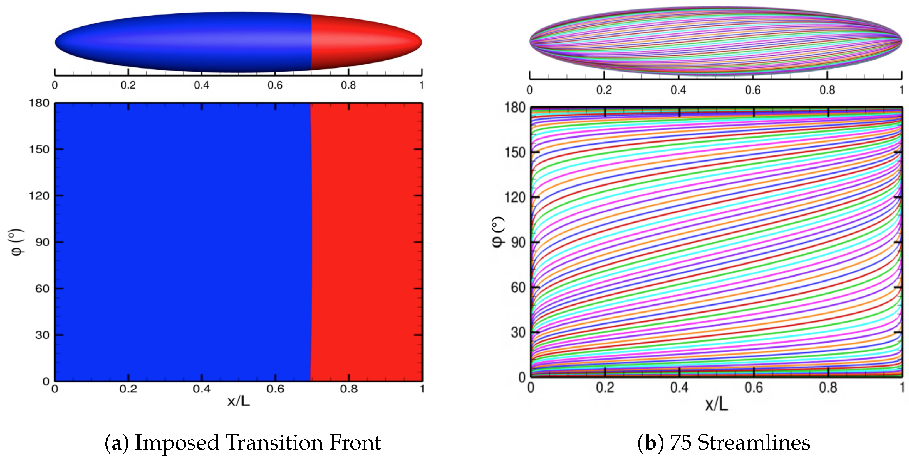
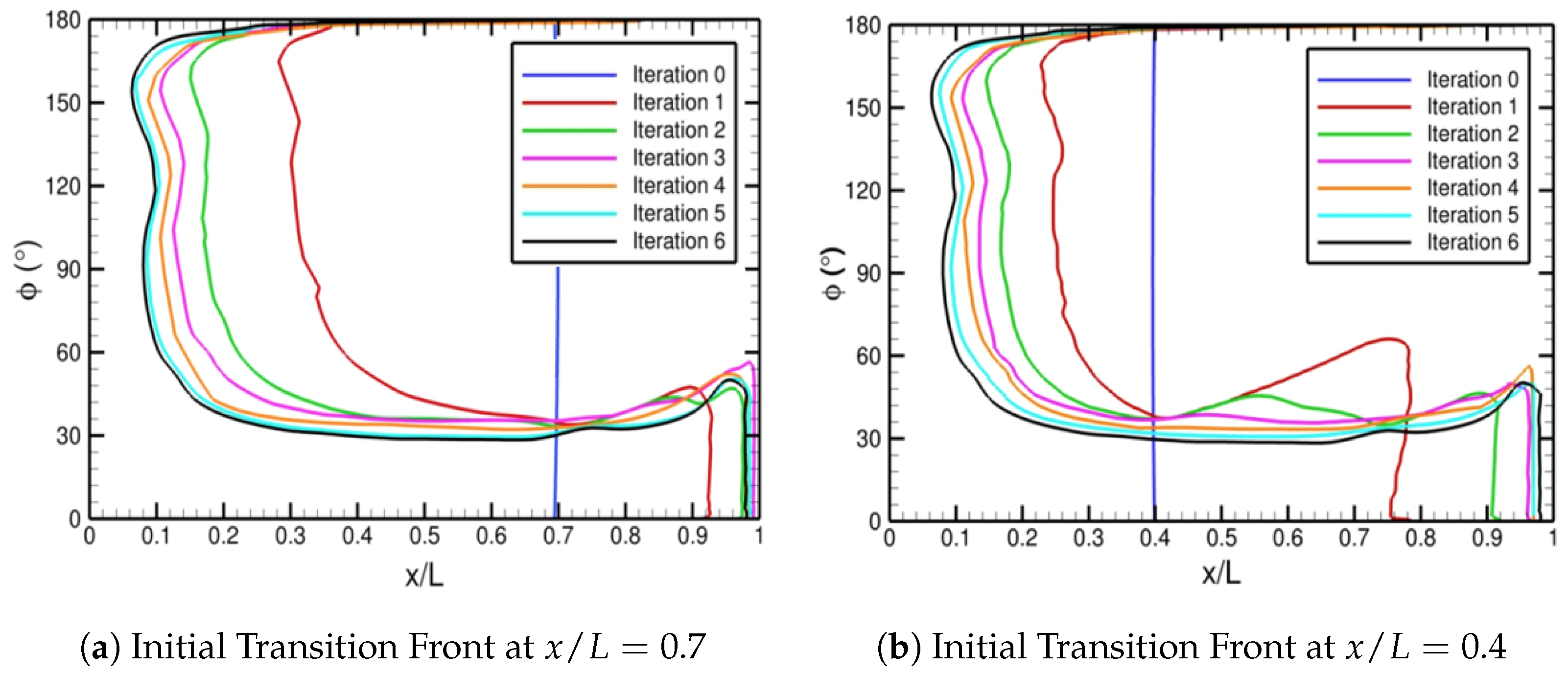
To initiate the automated FUN3D–LASTRAC method, we impose a transition front downstream at . This initial transition front is shown in Figure 14a, where the blue contours indicate a laminar region and the red contours indicate a turbulent region. For the LASTRAC stability analysis, we use 75 vertex seeds on the spheroid surface. The solver-independent module creates the streamlines for stability analysis from these vertex seeds. Figure 14b displays the 75 streamlines on the spheroid surface. We employ under-relaxation by using Equation (7) at each point along the azimuthal or plane with We use the dual – criterion [45,46,47] to determine where transition occurs from the TS and crossflow N-factor values. Refer to Choudhari et al. [2] for more information on calibrating the dual – criterion for multiple aerodynamic configurations. To illustrate the automated transition modeling for a 3D flow configuration, we use the simple criterion . In a real-world application, the criterion would be tuned for a specific facility using a broad range of data. Unlike for the 2D cases, we use point transition or an intermittency zone with zero length, which is a convenient option for 3D cases with mixed-mode transition where intermittency models have not been developed. Figure 15 displays the transition fronts corresponding to iterations 0 through 6 for two different initially imposed transition fronts. Notice that, by iteration 6, the automated FUN3D–LASTRAC method converges for both initial conditions.
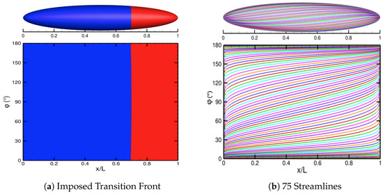
Figure 14.
Initial transition front imposed within the SA-neg model of the FUN3D solver on the left, where the color blue indicates a laminar region and the color red indicates a turbulent region. The streamline distribution on the 6:1 prolate spheroid for stability analysis with LASTRAC is displayed on the right.
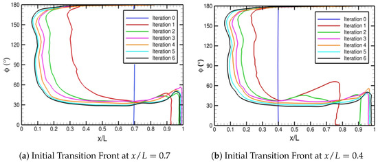
Figure 15.
Transition fronts corresponding to iterations 0 through 6 from the automated FUN3D–LASTRAC method for the 6:1 prolate spheroid with different initial fronts.
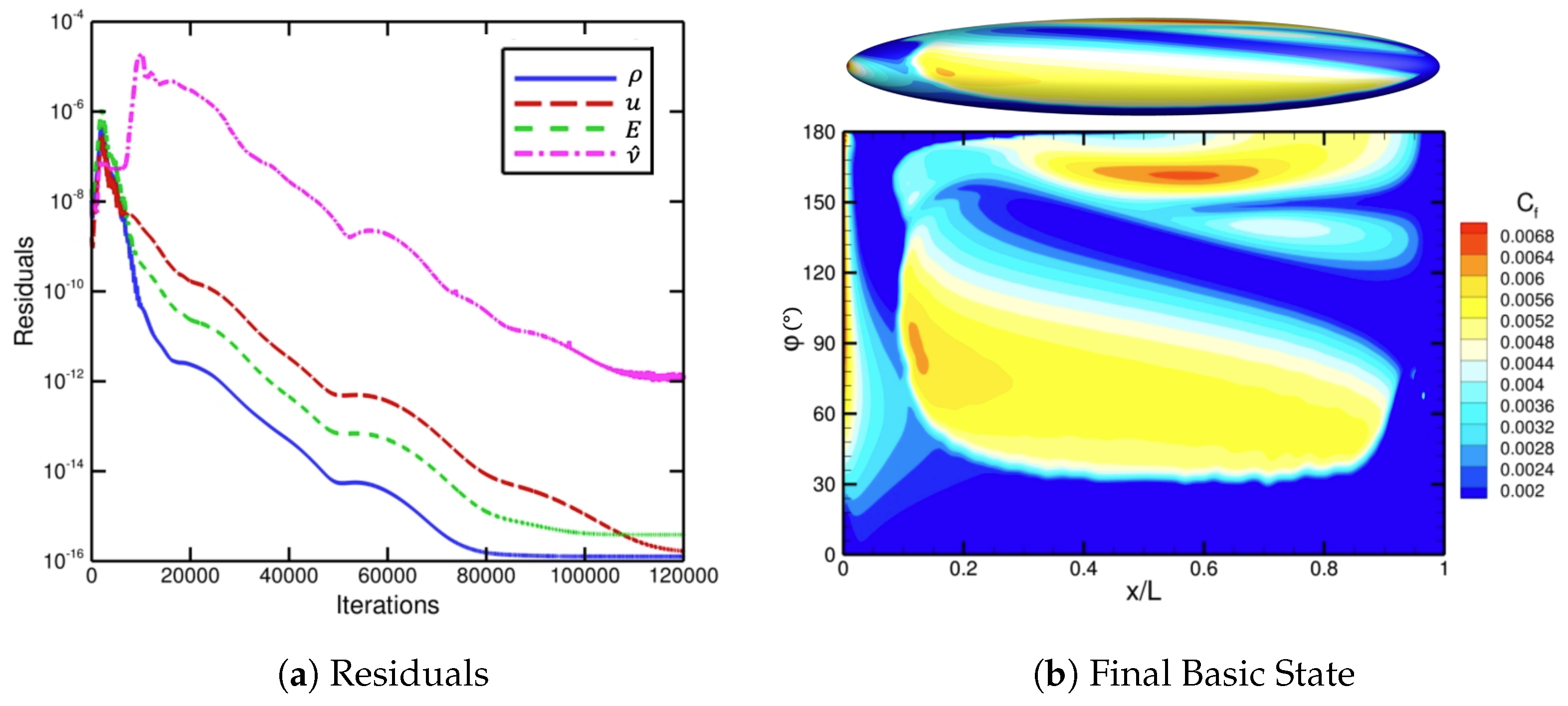
Figure 16 depicts the N-factor contours of TS and crossflow instability from PSE with LASTRAC. The final imposed transition front is also shown in Figure 16, downstream of which the N-factor contours are removed or set to zero because the flow has already transitioned to turbulence. For this case where , the N-factor values associated with TS waves are relatively small and do not significantly influence transition, except for far downstream near and in Figure 16a. Crossflow vortices are important for this angle of attack because the associated N-factor values are appreciably large and are likely to dominate transition for . We show the final solution of the automated FUN3D–LASTRAC method in Figure 17, along with the mean-flow basic-state residuals. Notice in Figure 17a that the mean-flow basic-state residuals drop approximately 10 orders of magnitude to machine zero and level out. The skin-friction contours of the final converged solution in Figure 17b are smooth and match the final transition front in Figure 15. Also, the results in Figure 17b agree with the skin-friction contours in Figure 11d of Krimmelbein et al. [44] for the 6:1 prolate spheroid at , computed using a coupled iterative approach (i.e., SST model [48] with a similar dual N-factor strategy).
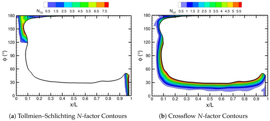
Figure 16.
TS and crossflow N-factor contours from PSE using LASTRAC for the 6:1 prolate spheroid with the final converged transition front.
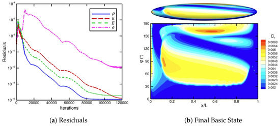
Figure 17.
Residuals and the final transitional solution from the automated FUN3D–LASTRAC method for the 6:1 prolate spheroid.
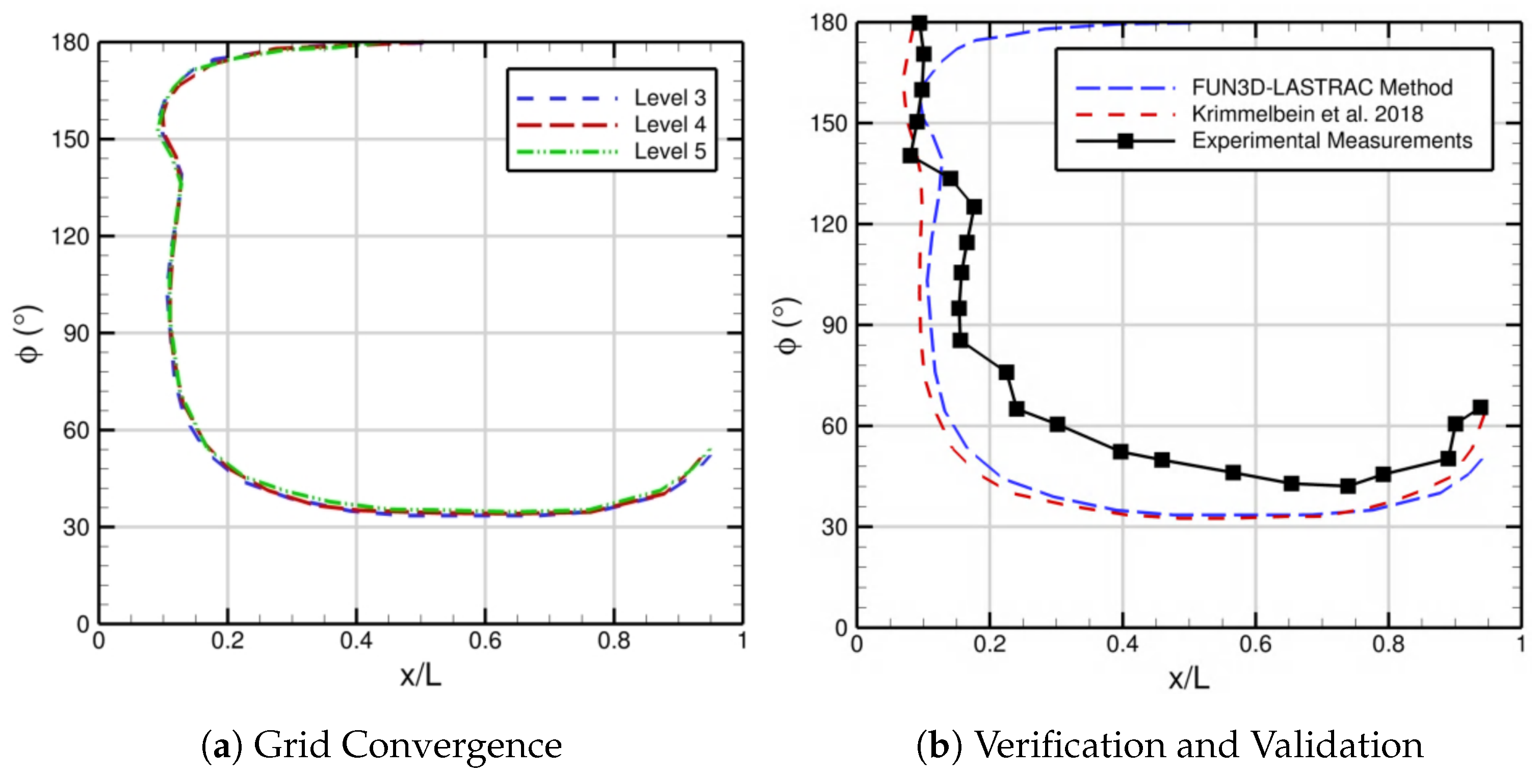
The grid convergence of the automated FUN3D–LASTRAC transition-prediction method is displayed in Figure 18a. Comparisons with the results from our method, the experimental measurements in Kreplin et al. [41], and the computational results from Krimmelbein et al. [44] based on the SST model paired with a similar dual N-factor strategy are depicted in Figure 18b. For the results in Figure 18, the extracted transition front comes from the skin-friction contours, more specifically . This is conducted for better comparison with the measurements by Kreplin et al. [41] and Krimmelbein et al. [44]. In Figure 18a, the converged transition front is relatively insensitive to changes in the grid resolution across levels three, four, and five. The agreement between our computational results and those of Krimmelbein et al. [44] is very good. The comparison between our predictions and the experimental measurements by Kreplin et al. [41] is also reasonable, except that the predicted transition front is more upstream across the crossflow-dominated region from , highlighting the need for calibrating the dual N-factor criterion in actual applications, similar to Krimmelbein et al. [44] and Choudhari et al. [2]. Overall, the sufficient iterative and grid convergence, along with the successful validation of the automated iterative coupled approach with FUN3D and LASTRAC for a 3D flow configuration, demonstrate that it can be applied to more complex problems and maintain accuracy, robustness, and efficiency.
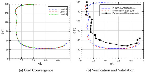
Figure 18.
Comparisons of the different transition fronts, i.e., isosurface contour line equal to 0.0030, from experimental measurements [41], the N-factor method with the SST turbulence model from Krimmelbein et al. [44], and our iterative method using FUN3D and LASTRAC.
4. Conclusions
The ability to accurately, robustly, and efficiently predict transition to turbulence in viscous flows is a key objective of the NASA CFD Vision 2030 initiative. In this article, we presented an automated iterative approach that couples two state-of-the-art capabilities: the unstructured flow solver FUN3D and the stability analysis code LASTRAC. This methodology was successfully demonstrated across a range of different transition scenarios in several canonical low-speed boundary-layer flows. These scenarios included natural transition via TS instabilities in zero-pressure-gradient flow over a flat plate, separation-bubble-induced transition over the NLF-0416 airfoil, and crossflow-dominated transition over a 6:1 prolate spheroid at a nonzero angle of incidence. The application of automated PSE-based stability analysis to these transition mechanisms in both 2D and 3D boundary layers represents a significant advancement over the traditional linear stability approaches by providing higher-fidelity modeling of the spatial evolution of the instability waves that initiate the transition process. The overall framework entails the application of three integrated software components during each iteration. First, a basic state computation is performed using steady-state RANS with the SA turbulence model in FUN3D that incorporates an estimated transition front. Second, boundary-layer stability analysis is conducted using the PSE implementation in LASTRAC to estimate the revised transition onset front. Third, a solver-independent module performs several critical functions that include viscous surface identification, the extraction of wall-normal profiles along selected disturbance growth paths, and the generation of integration trajectories (typically in the form of inviscid streamlines).
For the first test case, we simulated Mach 0.147 flow over a 2D zero-pressure-gradient flat plate, where natural boundary-layer transition occurs. The iterative approach coupling FUN3D and LASTRAC, along with a robust intermittency function, was shown to converge for two different fixed under-relaxation factors. This flat-plate case did not have significant viscous–inviscid interaction and, hence, was not significantly sensitive to iterative changes in the location of transition onset. Furthermore, grid convergence of the coupled approach with FUN3D and LASTRAC was also demonstrated for this flat-plate case, where consistent results were obtained for key metrics, including the drag coefficient, the location of transition onset, and the skin-friction coefficient. Our FUN3D–LASTRAC transition-prediction method showed good agreement with other methods that included an analogous approach coupling the overset grid flow solver OVERFLOW and LASTRAC, the SST2003-LM2009 and SA1994-AFT2014 models based on model auxiliary transport equations, and the Schubauer and Skramstad experiment [38] in terms of skin-friction evolution and the transition onset location.
The second test case involved the NLF-0416 airfoil at a five-degrees angle of attack. This configuration exhibited two distinct transition mechanisms: natural boundary-layer transition on the upper surface and separation-bubble-induced transition along the lower surface. Again, despite strong viscous–inviscid interaction due to the separation bubble that led to oscillations in the lower-surface transition location during early iterations, our coupled approach achieved successful convergence. The solution converged after five iterations, as evidenced by the convergence of the skin-friction distribution across the airfoil surface, the N-factor envelopes, and the predicted transition locations. A grid convergence study confirmed the reliability of the computed solution, demonstrating consistent predictions of the lift coefficient, drag coefficient, streamwise distribution of the skin-friction coefficient, and the transition onset locations on both upper and lower surfaces. The FUN3D–LASTRAC-based predictions of surface pressure distribution and transition onset locations showed excellent agreement with multiple verification sources, including the SST2003-LM2009 model, the SA1994-AFT2014 model, and the Somers experiment [40].
For the final test case, we simulated Mach 0.136 flow over a 6:1 prolate spheroid at an angle of attack equal to twenty-four degrees, where both TS waves and crossflow vortices had significant amplification factors. Thus, we employed a dual N-factor criterion based on PSE () to determine the transition front. The coupled FUN3D–LASTRAC approach converged iteratively using an under-relaxation factor of 0.7. Our analysis revealed distinct transition mechanisms across different regions of the spheroid surface. TS waves dominated for and , while crossflow instability played a dominant role across the intermediate region, . The converged transition front demonstrated insensitivity to changes in the resolution on finer grids. The verification of the FUN3D–LASTRAC coupling approach showed excellent agreement with the transition front predicted by Krimmelbein et al. [44] using a similar approach. A comparison of the predicted transition front with the available measurements also indicated acceptable agreement with the experimental data by Kreplin et al. [41]. These three test cases demonstrate that our automated PSE-based FUN3D–LASTRAC coupling approach reliably predicts transition in viscous flows with good iterative and grid convergence. Future applications across diverse flow configurations should help to refine the N-factor calibrations, advancing the transition modeling capabilities for the design of greener aircraft.
Author Contributions
N.H.: conceptualization, methodology, formal analysis, investigation, writing—original draft preparation, visualization. M.M.C.: conceptualization, investigation, resources, writing—review and editing, supervision, project administration, funding acquisition. F.L.: methodology, software, supervision, writing—review and editing. P.P.: methodology, investigation, supervision, writing—review and editing. B.S.V.: conceptualization, methodology, validation, data curation, writing—review and editing. All authors have read and agreed to the published version of the manuscript.
Funding
This research is funded by the Revolutionary Computational AeroSciences discipline under the Transformational Tools and Technologies Project of the NASA Transformative Aeronautics Concepts Program.
Data Availability Statement
Data will be made available on request.
Acknowledgments
The authors greatly appreciate computational resources from both the NASA Langley Research Center’s K Cluster and the NASA High-End Computing Program through the NASA Advanced Supercomputing Division at the NASA Ames Research Center.
Conflicts of Interest
Author Balaji S. Venkatachari was employed by the company Analytical Mechanics Associates, Inc. The remaining authors declare that the research was conducted in the absence of any commercial or financial relationships that could be construed as a potential conflict of interest.
References
- Slotnick, J.; Khodahoust, A.; Alonso, J.; Darmofal, D.; Gropp, W.; Mavriplis, D. CFD Vision 2030 Study: A Path to Revolutionary Computational Aerosciences; NASA/CR-2014-218178; NASA: Washington, DC, USA, 2014.
- Choudhari, M.M.; Beyak, E.; Hildebrand, N.; Li, F.; Vogel, E.; Srivastava, V.; Venkatachari, B.S. Transition Modeling in Support of CFD Vision 2030—Highlights of Recent Efforts at the NASA Langley Research Center. In Proceedings of the 34th Congress of the International Council of the Aeronautical Sciences, Florence, Italy, 9–13 September 2024. [Google Scholar]
- Schrauf, G. Status and Perspectives of Laminar Flow. Aeronaut. J. 2005, 109, 639–644. [Google Scholar] [CrossRef]
- Collier, F. Subsonic Fixed Wing Project Overview. In Proceedings of the NASA FAP 2008 Annual Meeting, Edwards, CA, USA, 7–9 October 2008. [Google Scholar]
- Langtry, R.B.; Menter, F.R. Correlation-based transition modeling for unstructured parallelized computational fluid dynamics codes. AIAA J. 2009, 47, 2894–2906. [Google Scholar] [CrossRef]
- Smith, A.; Gamberoni, A. Transition, Pressure Gradient, and Stability Theory; Report No. ES26388; Douglas Aircraft Co.: Santa Monica, CA, USA, 1956. [Google Scholar]
- Ingen, J.V. A Suggested Semi-Empirical Method for the Calculation of the Boundary Layer Transition Region; Report No. UTH1-74; University of Technology: Delft, The Netherlands, 1956. [Google Scholar]
- Mack, L. Transition prediction and linear stability theory. In Proceedings of the Laminar-Turbulent Transition, CP-224, AGARD, Copenhagen, Denmark, 2–4 May 1977; pp. 1–22. [Google Scholar]
- Crouch, J.D.; Ng, L. Variable N-Factor Method for Transition Prediction in Three-Dimensional Boundary Layers. AIAA J. 2000, 38, 211–216. [Google Scholar] [CrossRef]
- Herbert, T. Parabolized stability equations. Annu. Rev. Fluid Mech. 1997, 29, 245–283. [Google Scholar] [CrossRef]
- Malik, M.; Liao, W.; Li, F.; Choudhari, M.M. Discrete-Roughness-Element-Enhanced Swept-Wing Natural Laminar Flow at High Reynolds Number. AIAA J. 2015, 53, 2321–2334. [Google Scholar] [CrossRef]
- Menter, F.R.; Langtry, R.B.; Völker, S. Transition Modelling for General Purpose CFD Codes. J. Flow Turbul. Combust. 2006, 77, 277–303. [Google Scholar] [CrossRef]
- Perraud, J.; Arnal, D.; Casalis, G.; Archambaud, J.-P.; Donelli, R. Automatic Transition Predictions Using Simplified Methods. AIAA J. 2009, 47, 2676–2684. [Google Scholar] [CrossRef]
- Coder, J.G.; Maughmer, M.D. Computational Fluid Dynamics Compatible Transition Modeling Using an Amplification Factor Transport Equation. AIAA J. 2014, 52, 2506–2512. [Google Scholar] [CrossRef]
- Krumbein, A.; Krimmelbein, N.; Grabe, C. Streamline-Based Transition Prediction Techniques in an Unstructured Computational Fluid Dynamics Code. AIAA J. 2017, 55, 1548–1564. [Google Scholar] [CrossRef]
- Halila, G.L.O.; Chen, G.; Shi, Y.; Fidkowski, K.J.; Martins, J.R.R.A.; Mendonça, M.T. High-Reynolds Number Transitional Flow Prediction Using a Coupled Discontinuous-Galerkin RANS PSE Framework; AIAA Paper 2019-0974; AIAA: Reston, VA, USA, 2019. [Google Scholar] [CrossRef]
- Halila, G.L.O.; Fidkowski, K.J.; Martins, J.R.R.A. Toward Automatic Parabolized Stability Equation-Based Transition-to-Turbulence Prediction for Aerodynamic Flows. AIAA J. 2020, 59, 462–473. [Google Scholar] [CrossRef]
- Drela, M.; Giles, M.B. Viscous-Inviscid Analysis of Transonic and Low Reynolds Number Airfoils. AIAA J. 1987, 25, 1347–1355. [Google Scholar] [CrossRef]
- Sturdza, P. An Aerodynamic Design Method for Supersonic Natural Laminar Flow Aircraft. Ph. D. Thesis, Stanford University, Stanford, CA, USA, 2003. [Google Scholar]
- Davis, M.B.; Reed, H.L.; Youngren, H.; Smith, B.; Bender, E. Transition Prediction Method Review Summary for the Rapid Assessment Tool for Transition Prediction (RATTraP); Technical Report AFRL-VA-WP-TR-2005-3130; Air Force Research Lab, Wright-Patterson AFB: Riverside, OH, USA, 2005. [Google Scholar]
- Cliquet, J.; Houdeville, R.; Arnal, D. Application of Laminar-Turbulent Transition Criteria in Navier-Stokes Computations. AIAA J. 2008, 46, 1182–1190. [Google Scholar] [CrossRef]
- Kosarev, L.; Séror, S.; Lifshitz, Y. Parabolized Stability Equations Code with Automatic Inflow for Swept Wing Transition Analysis. J. Aircr. 2016, 53, 1647–1669. [Google Scholar] [CrossRef]
- Anderson, W.K.; Bonhaus, D.L. An implicit upwind algorithm for computing turbulent flows on unstructured grids. Comput. Fluids 1994, 23, 1–22. [Google Scholar] [CrossRef]
- Chang, C.L. Langley Stability and Transition Analysis Code (LASTRAC) Version 1.2 User Manual. NASA TM-2004-213233. 2004. Available online: https://ntrs.nasa.gov/search.jsp?R=20040082550 (accessed on 20 March 2025).
- Park, M.A. Anisotropic Output-Based Adaptation with Tetrahedral Cut Cells for Compressible Flows. Ph.D. Thesis, Massachusetts Institute of Technology, Cambridge, MA, USA, September 2008. [Google Scholar]
- Park, M.A.; Balan, A.; Clerici, F.; Alauzet, F.; Loseille, A.; Kamenetskiy, D.; Krakos, J.A.; Michal, T.; Galbraith, M.C. Verification of Viscous Goal-Based Anisotropic Mesh Adaptation; AIAA Paper 2021-1362; AIAA: Reston, VA, USA, 2021. [Google Scholar] [CrossRef]
- Nielsen, E.J.; Lu, J.; Park, M.A.; Darmofal, D.L. An Implicit, Exact Dual Adjoint Solution Method for Turbulent Flows on Unstructured Grids. Comput. Fluids 2004, 33, 1131–1155. [Google Scholar] [CrossRef]
- Nielsen, E.J.; Diskin, B. Discrete Adjoint-Based Design for Unsteady Turbulent Flows on Dynamic Overset Unstructured Grids. AIAA J. 2013, 51, 1355–1373. [Google Scholar] [CrossRef]
- Venkatachari, B.S.; Carnes, J.A.; Chang, C.L.; Choudhari, M.M. Boundary-Layer Transition Prediction Through Loose Coupling of OVERFLOW and LASTRAC; AIAA Paper 2022-3682; AIAA: Reston, VA, USA, 2023. [Google Scholar] [CrossRef]
- Hildebrand, N.; Chang, C.L.; Choudhari, M.M.; Li, F.; Nielsen, E.J.; Venkatachari, B.S.; Paredes, P. Coupling of the FUN3D Unstructured Flow Solver and the LASTRAC Stability Code to Model Transition; AIAA Paper 2022-1952; AIAA: Reston, VA, USA, 2022. [Google Scholar] [CrossRef]
- Anderson, W.K.; Biedron, R.T.; Carlson, J.R.; Derlaga, J.M.; Diskin, B.; Druyor, C.T.; Gnoffo, P.A.; Hammond, D.P.; Jacobson, K.E.; Jones, W.T.; et al. FUN3D Manual: 14.0.2; NASA TM 20230004211; NASA Langley Research Center: Hampton, VA, USA, 2022.
- Spalart, P.R.; Allmaras, S.R. A One-Equation Turbulence Model for Aerodynamic Flows. Rech. Aerosp. 1994, 1, 5–21. [Google Scholar]
- Roe, P.L. Approximate Riemann Solvers, Parameter Vectors, and Difference Schemes. J. Comput. Phys. 1981, 43, 357–372. [Google Scholar] [CrossRef]
- Dhawan, S.; Narasimha, R. Some Properties of Boundary Layer Flow During the Transition from Laminar to Turbulent Motion. J. Fluid Mech. 1958, 3, 418–436. [Google Scholar] [CrossRef]
- Krumbein, A. Transition Flow Modeling and Application Fo High-Lift Multi-Element Airfoil Configurations. J. Aircr. 2003, 40, 786–794. [Google Scholar] [CrossRef]
- Chang, C.L. LASTRAC.3d: Transition Prediction in 3D Boundary Layers; AIAA Paper 2004-2542; AIAA: Reston, VA, USA, 2004. [Google Scholar] [CrossRef]
- Chang, C.L. Development of Physics-Based Transition Models for Unstructured-Mesh CFD Codes Using Deep Learning Models; AIAA Paper 2021-2828; AIAA: Reston, VA, USA, 2021. [Google Scholar] [CrossRef]
- Schubauer, G.B.; Skramstad, H.K. Laminar Boundary-Layer Oscillations and Stability of Laminar Flow. J. Aeronaut. Sci. 1947, 14, 69–78. [Google Scholar] [CrossRef]
- Venkatachari, B.S.; Denison, M.; Mysore, P.V.; Hildebrand, N.; Choudhari, M.M. Verification of the γ-Reθt Transition Model in OVERFLOW and FUN3D. J. Aircr. 2024, 61, 345–364. [Google Scholar] [CrossRef]
- Somers, D.M. Design and Experimental Results for a Natural-Laminar-Flow Airfoil for General Aviation Applications; NASA-TP-1861; NASA: Washington, DC, USA, 1981.
- Kreplin, H.P.; Vollmers, H.; Meier, H.U. Wall Shear Stress Measurements on an Inclined Prolate Spheroid in the DFVLR 3M × 3M Low Speed Wind Tunnel; Data Report DFVLR 1B 222-84/A33; Göttingen, Germany, 1985. [Google Scholar]
- Spall, R.E.; Malik, M.R. Linear Stability of Three-Dimensional Boundary Layers over Axisymmetric Bodies at Incidence. AIAA J. 1992, 30, 905–913. [Google Scholar] [CrossRef]
- Stock, H.W.; Haase, W. Navier-Stokes Airfoil Computations with eN Transition Prediction Including Transitional Flow Regions. AIAA J. 2000, 38, 2059–2066. [Google Scholar] [CrossRef]
- Krimmelbein, N.; Krumbein, A.; Grabe, C. Validation of Transition Modeling Techniques for a Simplified Fuselage Configuration; AIAA Paper 2018-0030; AIAA: Reston, VA, USA, 2018. [Google Scholar] [CrossRef]
- Horstmann, K.; Redeker, G.; Quast, A.; Dressler, U.; Bieler, H. Flight Test with a Natural Laminar Flow Glove on a Transport Aircraft; AIAA Paper 1990-3044; AIAA: Reston, VA, USA, 1990. [Google Scholar] [CrossRef]
- Arnal, D. Boundary Layer Transition: Prediction Based on Linear Theory; Special course on Progress in Transition Modeling, AGARD. R-793; Specialised Printing Services Limited: Loughton, UK, 1994. [Google Scholar]
- Paredes, P.; Venkatachari, B.; Choudhari, M.M.; Li, F.; Hildebrand, N.; Chang, C.L. Transition Analysis for the CRM-NLF Wind Tunnel Configuration; AIAA Paper 2021-1431; AIAA: Reston, VA, USA, 2021. [Google Scholar] [CrossRef]
- Menter, F.R. Two-equation eddy-viscosity turbulence models for engineering applications. AIAA J. 1994, 32, 1598–1605. [Google Scholar] [CrossRef]


Disclaimer/Publisher’s Note: The statements, opinions and data contained in all publications are solely those of the individual author(s) and contributor(s) and not of MDPI and/or the editor(s). MDPI and/or the editor(s) disclaim responsibility for any injury to people or property resulting from any ideas, methods, instructions or products referred to in the content. |
© 2025 by the authors. Licensee MDPI, Basel, Switzerland. This article is an open access article distributed under the terms and conditions of the Creative Commons Attribution (CC BY) license (https://creativecommons.org/licenses/by/4.0/).