Simulation of Antiplane Piezoelectricity Problems with Multiple Inclusions by the Meshless Method of Fundamental Solution with the LOOCV Algorithm for Determining Sources

Abstract

This paper provides a high-accuracy and efficient method for addressing antiplane piezoelectricity problems with multiple inclusions. The method of fundamental solutions is a boundary-type meshless method that applies the linear combination of fundamental solutions as approximate solutions with the collocation method for determining the unknowns. To avoid the singularity of fundamental solutions, sources are placed away from the physical boundary. The leave-one-out cross-validation algorithm is employed to identify the optimal source placements to mitigate the influence of this singularity on numerical results. Numerical results of the stress concentration and electric field concentration at the interface between circular and elliptic inclusions and matrix are studied and compared well with references. Furthermore, the stability of the method is verified. Perturbations are added to the boundary conditions. Accuracy on the order of 10⁻¹¹ is obtained without noise. After adding the disturbance, the calculation accuracy is the same order of magnitude as the disturbance.

1. Introduction

Due to the electro-mechanical coupling phenomenon, piezoelectric materials deform and generate an electric field when subjected to deformation. This inherent electro-mechanical behavior makes piezoelectric materials extensively employed in intelligent structures and devices, such as sensors and actuators. The common piezoelectric materials are piezoelectric ceramics and have been widely used. However, piezoelectric materials may possess initial defects such as cavities, inclusions, and cracks. Additionally, defects will occur when piezoelectric materials undergo certain processes or are subjected to specific conditions in the operating state. The presence of these defects will lead to the concentration of stress and electric field, thereby disabling the device. Consequently, the study of various types of defects in piezoelectric materials from the perspective of electro-mechanical coupling has garnered significant attention from material and mechanical professionals.

In this way, many research achievements need to be mentioned. Bleustein [1] discovered Bleustein waves in piezoelectric materials. Pak [2] analyzed a circle inclusion embedded in an infinite piezoelectric matrix within the framework of linear piezoelectricity and obtained an analytical solution for the case of a far-field antiplane mechanical load and a far-field in-plane electric load. Honein et al. [3] derived universal formulae at the point of contact of two circular piezoelectric fibers subjected to out-of-plane displacement and in-plane electric field. Chao et al. [4] examined the issue of multiple piezoelectric inclusions using complex variable theory and the method of successive approximations. Wu et al. [5] derived the electro-elastic field of an infinite piezoelectric medium containing two piezoelectric circular cylindrical inclusions using conformal mapping and the theorem of analytic continuation. Chen et al. [6] addressed the piezoelectric problem involving circular inclusions through a null-field approach. Chen et al. [7] utilized the subtracting and adding-back technique known as the regularized meshless method (RMM) to solve antiplane piezoelectricity problems with multiple inclusions. Yu et al. [8] studied antiplane piezoelectricity problems with multiple inclusions through the generalized finite difference method. In practical engineering applications, defects can take various forms. Therefore, researchers have focused on studying and evaluating more complex and more detrimental types of defects, such as elliptical-type defects. Pak [9] used the conformal mapping technique to analyze an elliptical piezoelectric inclusion embedded in an infinite piezoelectric matrix and obtained a closed-form solution. Mishra et al. [10] studied the distribution law of stress field and electric field of applied load at any loading angle, obtaining the energy release rates of self-similarly expanding and rotating defects in the presence of an electric field as a function of the loading angle. Lee et al. [11] employed a null-field integral approach to solve the problems of arbitrary location, different orientations, various sizes, and any number of elliptical holes and/or inhomogeneities embedded in an isotropic and infinite medium. Yu et al. [8] studied elliptical inclusions by the generalized finite difference method. These theoretical and numerical studies contribute to the understanding and advancement of piezoelectric materials and their applications in various fields.

With the advancement of numerical techniques and the enhancement of computing power, meshless methods have gained significant popularity in recent decades, particularly the boundary-type meshless method. These meshless methods can be formulated within the general framework of radial basis function collocation techniques. The method of fundamental solution (MFS) is a typical boundary-type meshless method. Kupradze et al. [12] first proposed the MFS and applied it to certain boundary value problems. The MFS has been fully developed over several decades and is extensively used for the solution of partial differential equations for which fundamental solutions exist. Nevertheless, the positioning of the source points is a crucial matter in MFS. The systems of equations can become highly ill-conditioned if the source nodes are not well placed. Hence, the accuracy of the MFS solution significantly relies on the location of source points. Scholars have noticed this problem and carried out a series of studies, e.g., [13,14,15]. Ling et al. [16] put forward the adaptive method employing a greedy algorithm for the selection of the sources for the Laplace equation. Tsai [17] discovered that when the condition number approaches the limit of the equation solver, the accuracy of MFS is precise. Liu [18] proposed a method to select the source points with multiple lengths which are solved from an uncoupled system of nonlinear algebraic equations. Wang et al. [19] derived a new merit function, namely the energy gap function, whose minimum leads to the optimal distribution of source points. Lin et al. [20] proposed the ghost points method to select the interval of the shape parameter using the radial basis function (RBF) in MFS. Zhang et al. [21] proposed new algorithms using two pseudo radial lines to seek source nodes in MFS, solving Laplace’s equation. Chen [22] observed that the effective condition number is associated with the shape parameter of RBF, the number of collocation points, and the error. In this paper, based on the MFS, the leave-one-out cross-validation (LOOCV) algorithm is used to identify the optimal location of the source points mainly because of its efficient computation. This algorithm is proposed by Rippa [23] for obtaining the shape parameter in the approximation of functions by linear combinations of RBFs. Fasshauer et al. [24] developed and applied the LOOCV algorithm to iterate approximate moving least square approximation and the solution of partial differential equations using RBF pseudo-spectral methods. Chen [25] obtained the location of source points in MFS for harmonic problems and also biharmonic problems based on the LOOCV algorithm. With the merits of MFS and the LOOCV algorithm, in this paper, we proposed a meshless method to solve the antiplane piezoelectricity problem and multiple inclusions with different shape boundaries embedded in an infinite matrix. In this problem, the multiple-domain approach is used to construct linear equations. The parameters optimized by the LOOCV algorithm need to determine the source points of interior and exterior problems at the same time. The distance between the source points and the collocation points is selected as the optimization parameter for the inclusion of a circular boundary. For the inclusion of an elliptical boundary, the fictitious boundary is scaled up or down the physical boundary. Source points are distributed on the fictitious boundary. The LOOCV algorithm optimizes this scale to identify the locations of source points.

The remainder of this paper is structured as follows. The statement of the antiplane piezoelectricity problems and the numerical strategy of the MFS employing the LOOCV algorithm are presented in Section 2. In Section 3, several numerical examples encompassing the tangential electric field distribution and stress concentration for diverse ratios of piezoelectric modulus are investigated to demonstrate the validity of the approach. Finally, the conclusion of this paper is provided in Section 4.

2. Problem Statement of Antiplane Piezoelectricity Problem and Formulation of MFS Using LOOCV Algorithm

2.1. Antiplane Piezoelectricity Problem

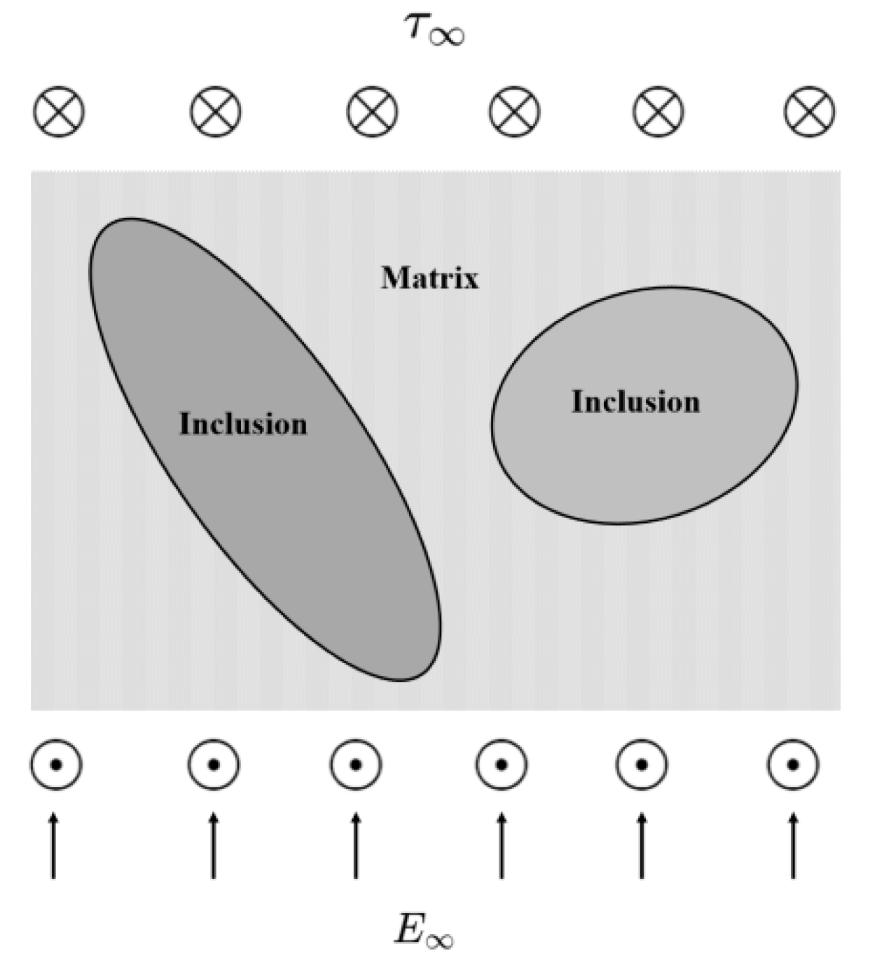
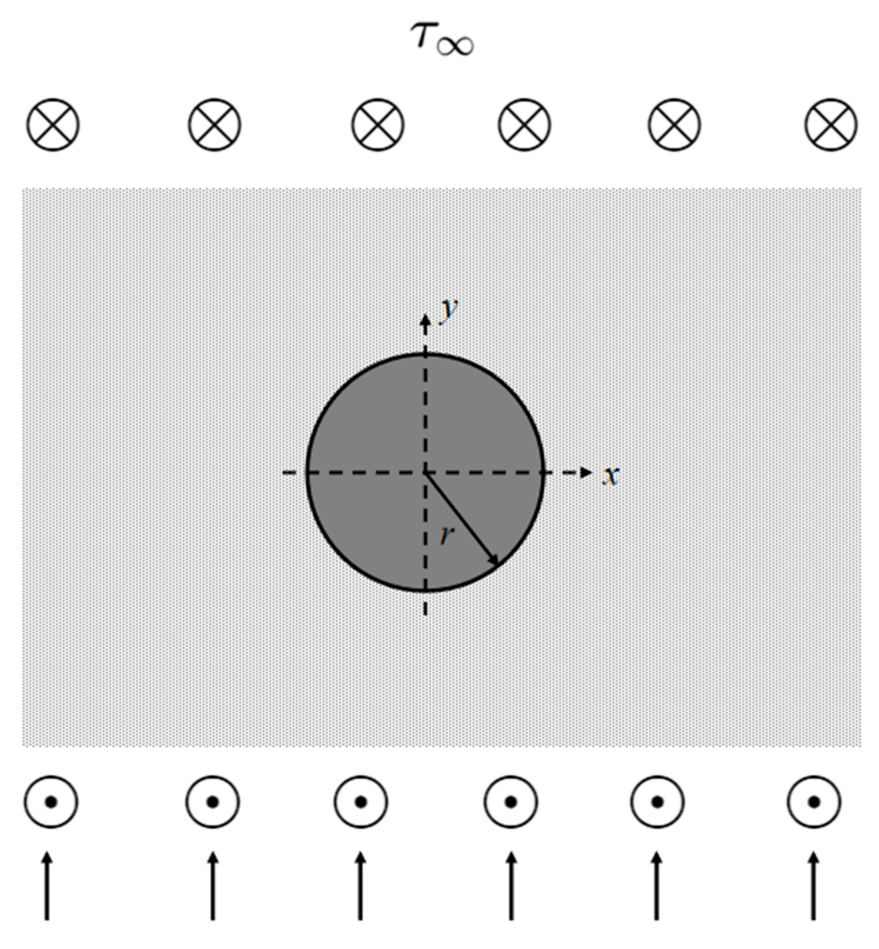
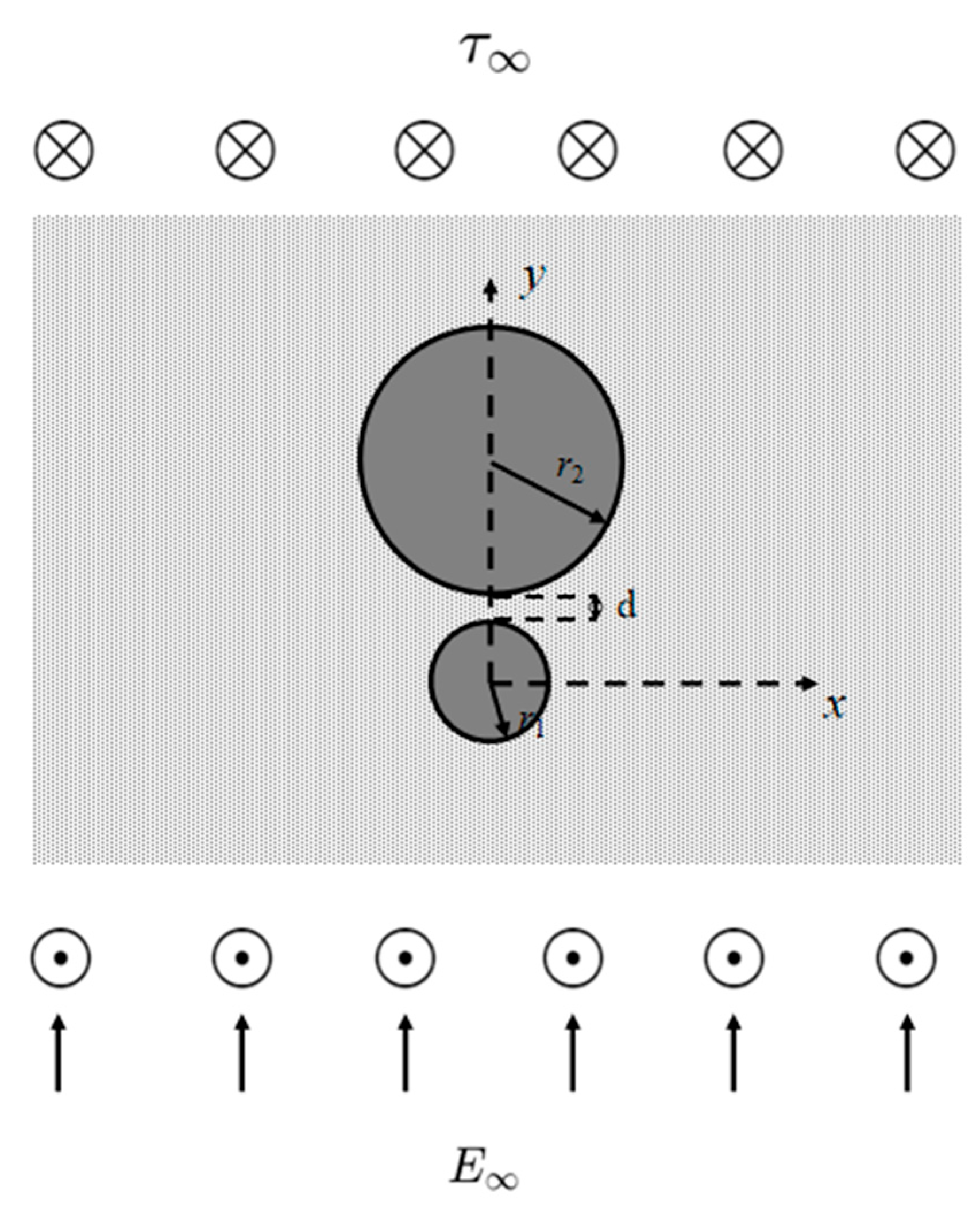
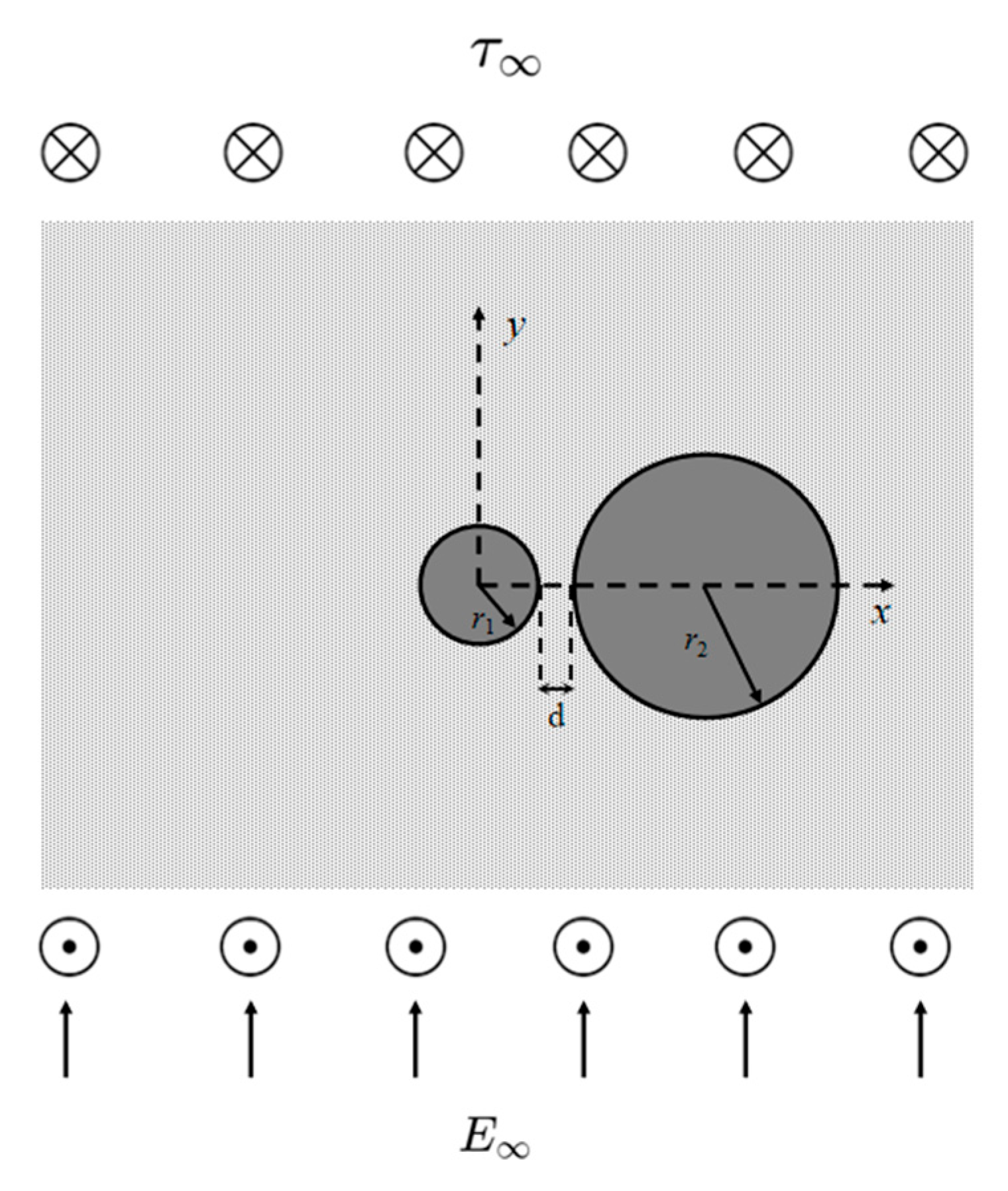
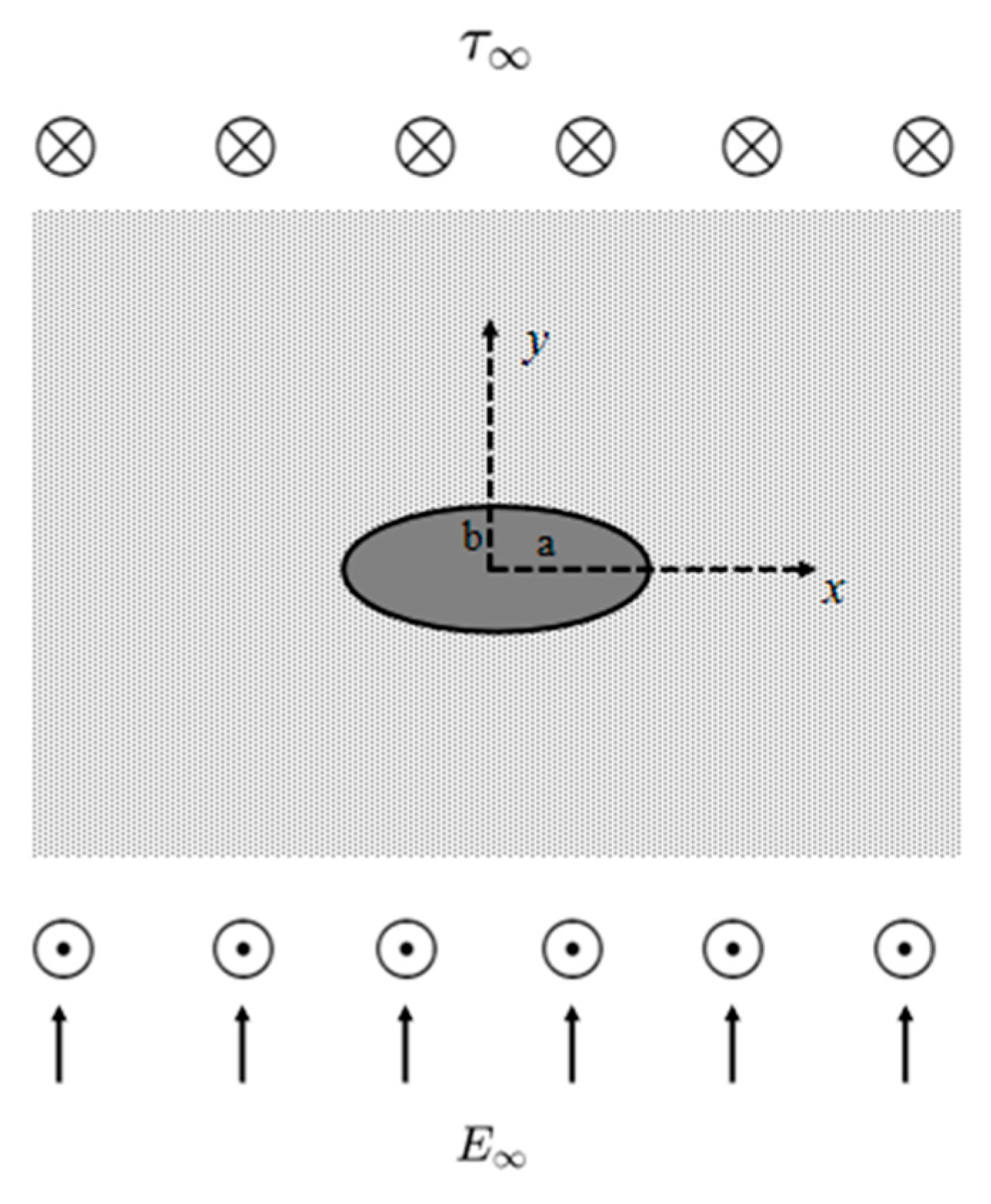
In this problem, the circular piezoelectric inclusions are embedded within another infinite piezoelectric matrix, as illustrated in Figure 1. A strong electric field polarizes the piezoelectric material. The material characteristics of each circular inclusion vary from those of the matrix. It is assumed that they possess the same materia orientation in the z-direction. The matrix is exposed to a remote antiplane shear ${\sigma }_{\infty }$ and a remote in-plane electric field $E_{\infty }$.

Taking the plane normal to the poling direction as the plane of interest, only the antiplane displacement $w$ couples with the in-plane electric field $E$, so that $u=v=0$, $w=w(x,y)$, $\varphi =\varphi (x,y)$. Without taking the body forces and body charges into account, the equilibrium equations are as follows

$${\displaystyle \frac{\partial {\sigma }_{zx}}{\partial x}}+{\displaystyle \frac{\partial {\sigma }_{zy}}{\partial y}}=0,$$

(1)

$${\displaystyle \frac{\partial D_x}{\partial x}}+{\displaystyle \frac{\partial D_y}{\partial y}}=0,$$

(2)

where ${\sigma }_{zx}$ and ${\sigma }_{zy}$ indicate the shear stress, while $D_x$ and $D_y$ represent the electric displacement. The constitutive equations for the coupling between the elastic fields and the electrical fields are formulated as below

$${\sigma }_{zx}=c_{44}{\gamma }_{zx}-e_{15}{E}_x,$$

(3)

$${\sigma }_{zy}=c_{44}{\gamma }_{zy}-e_{15}{E}_y,$$

(4)

$$D_x=e_{15}{\gamma }_{zx}+{\epsilon }_{11}{E}_x,$$

(5)

$$D_y=e_{15}{\gamma }_{zy}+{\epsilon }_{11}{E}_y,$$

(6)

where $c_{44}$ denotes the elastic modulus, ${\epsilon }_{11}$ is the dielectric modulus, and $e_{15}$ is the piezoelectric modulus. The ${\gamma }_{zx}$ and ${\gamma }_{zy}$ are the antiplane shear strain, while $E_x$ and $E_y$ are the in-plane electric field, which are defined as follows

$${\gamma }_{zx}={\displaystyle \frac{\partial u}{\partial x}},$$

(7)

$${\gamma }_{zy}={\displaystyle \frac{\partial u}{\partial y}},$$

(8)

$$E_x=-{\displaystyle \frac{\partial \phi }{\partial x}},$$

(9)

$$E_y=-{\displaystyle \frac{\partial \phi }{\partial y}}.$$

(10)

By substituting Equations (3)–(10) into Equations (1) and (2), the governing equations are simplified as

$$c_{44}\Delta w+e_{15}\Delta \varphi =0,$$

(11)

$$e_{15}\Delta w-{\epsilon }_{11}\Delta \varphi =0.$$

(12)

From Equations (11) and (12), we can obtain the equations as

$$\Delta w=0,$$

(13)

$$\Delta \varphi =0.$$

(14)

The continuity conditions at the interface between inclusions and the matrix are

$$w^m=w^i,$$

(15)

$${\varphi }^m={\varphi }^i,$$

(16)

$${\sigma }_{zr}^m=-{\sigma }_{zr}^i,$$

(17)

$$D_r^m=-D_r^i.$$

(18)

2.2. Method of Fundamental Solutions

The solution of the proposed problem is represented as the linear combination of fundamental solutions with unknown coefficients. This proposed linear combination is substituted back to the boundary conditions to obtain the unknown coefficients. The approximate solution to Equations (13) and (14) for the multiple inclusions problem is expressed as

$$u(x_i)={\displaystyle \sum _{j=1}^N{a}_{j}G(x_i},s_j), i=1,2,\dots M,$$

(19)

$$g(x_i)={\displaystyle \sum _{j=1}^N{a}_{j}H(}{x}_i,s_j), i=1,2,\dots M,$$

(20)

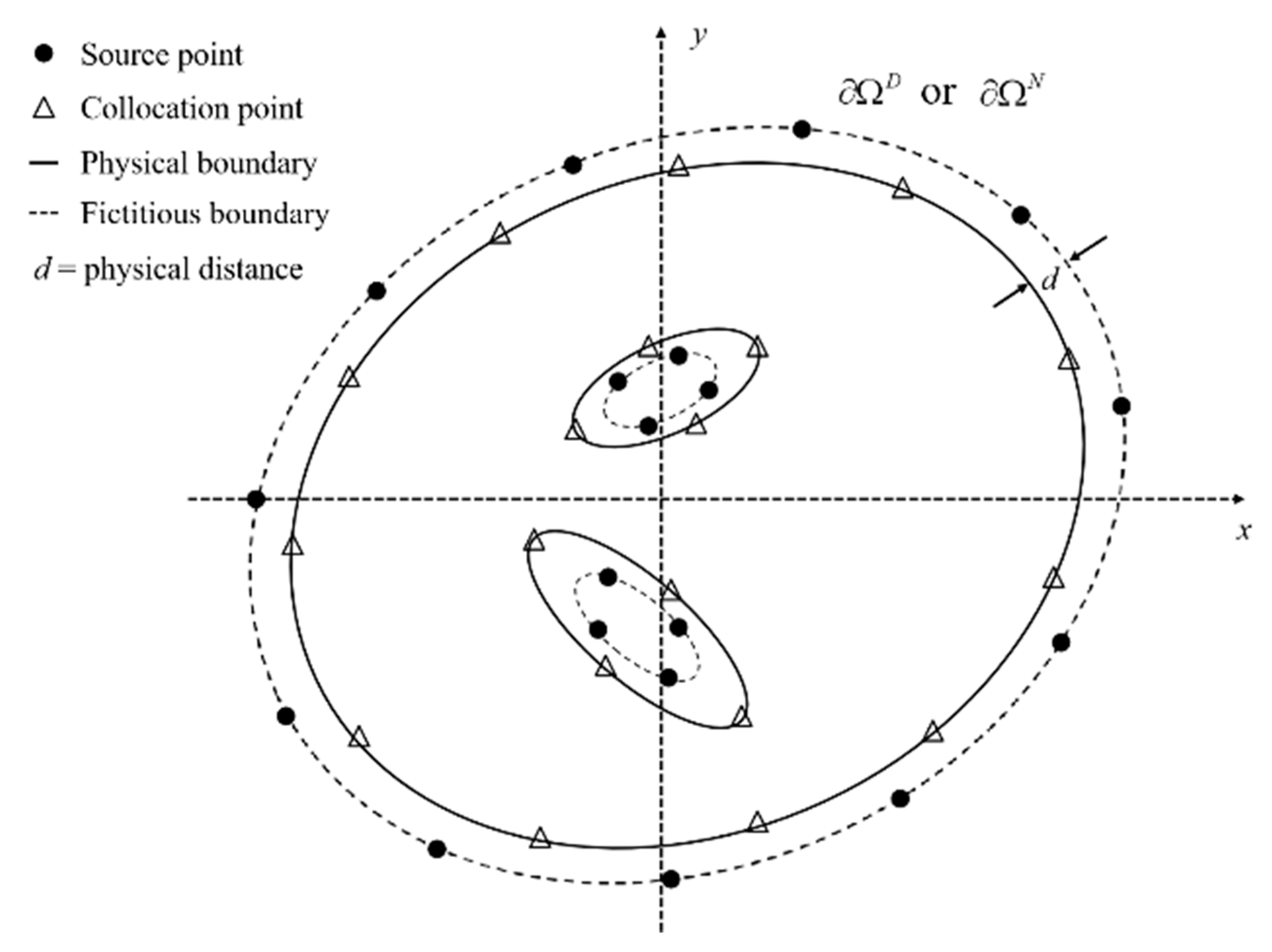
where $G\left(x_i,s_j\right)={\displaystyle \frac{1}{2\pi }}\ln r(x_i,s_j)$ is the fundamental solution of the Laplace equation of Equations (13) and (14), $r(s_j,x_i)=\left|\right|x_i-s_j\left|\right|$ denotes the Euclidean distance between the $i\mathrm{th}$ collocation point and $j\mathrm{th}$ source point. The source points $s_j$ are placed on the fictitious boundaries which are away from the physical boundaries to avoid the singularity of the fundamental solutions, which are shown in Figure 2 as an example. $u(x_i)$ can be considered as $w(x_i)$ or $\varphi (x_i)$ with the same formulation of different unknown coefficients. $a_j$ are the unknown coefficients (strength of singularity), while the strengths ${\left\{a_j\right\}}_{j=1}^N$ are determined by enforcing the approximations satisfying the boundary conditions (Dirichlet boundary conditions or Neumann boundary conditions). $N$ is the number of source points on the fictitious boundaries, while $M$ is the number of collocation points on the physical boundaries. $g(x_i)=n(x_i)\nabla u(x_i)$, and $H(x_i,s_j)=n(x_i)\nabla G(x_i,s_j)$, where $n(x_i)$ is the outward normal vector at $x_i$.

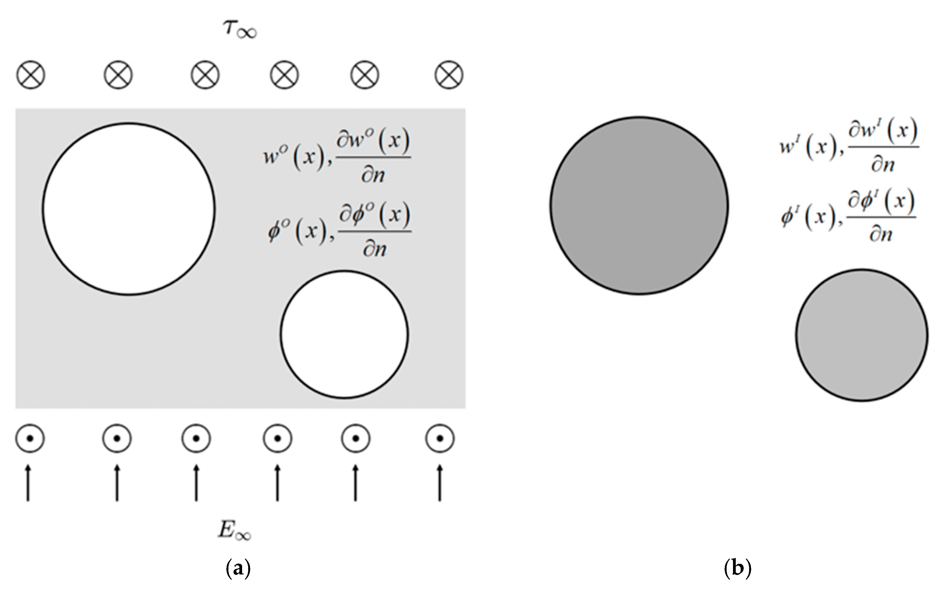
The problem of antiplane piezoelectricity with multiple inclusions is divided into two parts by a multiple-domain approach. One is an infinite matrix with circular holes, and the other is each circular inclusion, as shown in Figure 3a,b. The boundary data fulfill the interface conditions between matrix and inclusion, as presented in Equations (15)–(18).

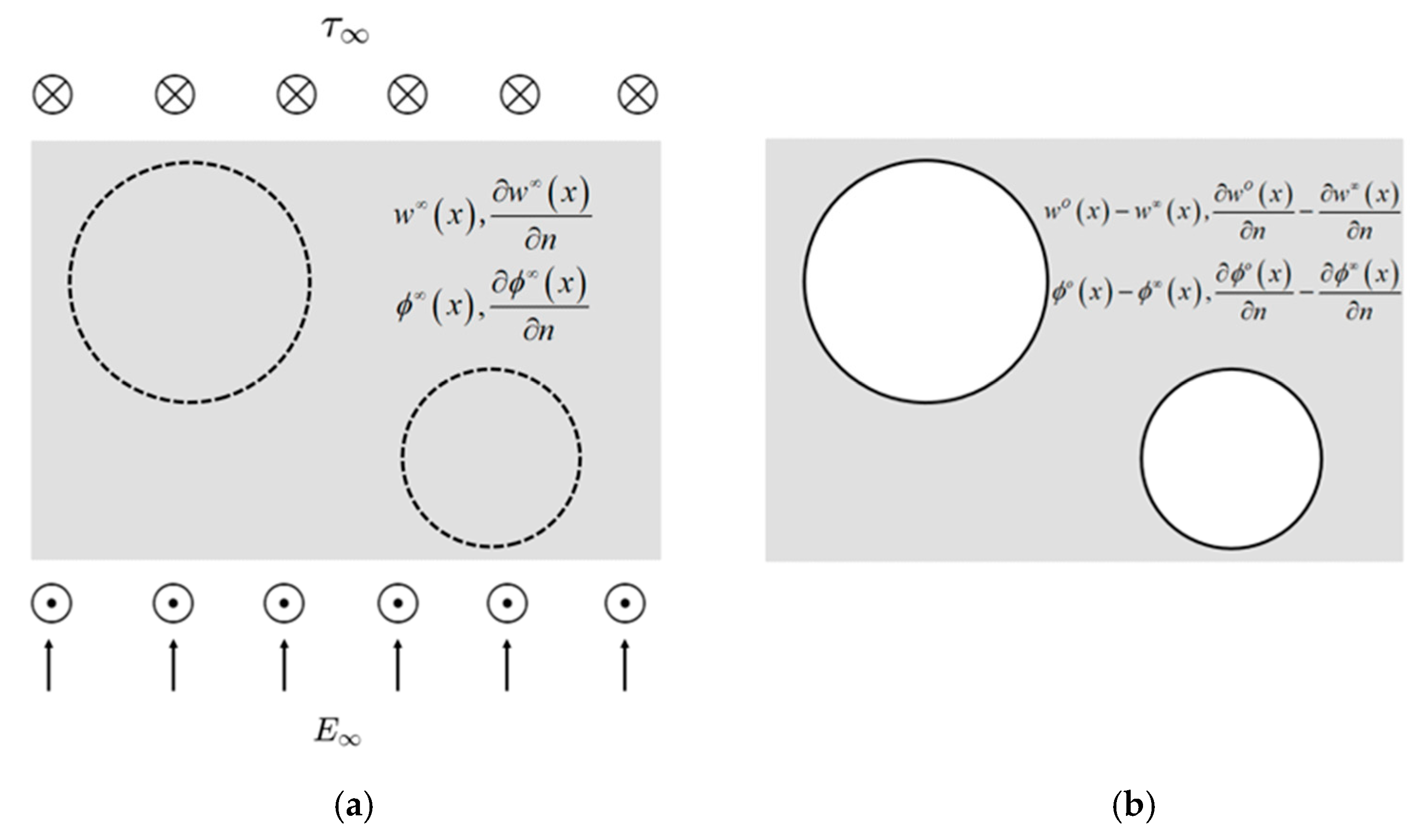
Moreover, the problem in Figure 3a can be decomposed into two parts, as shown in Figure 4a,b. One is an infinite matrix subjected to a far-field shear and far-field electric field, and the other is a finite matrix with circular holes. The exterior problem for the matrix is shown in Figure 4b, and the interior problem for inclusions is shown in Figure 3b, which are formulated by the MFS in a unified manner.

The solution expression of interior problem $(w(x_i^I))$, $(\varphi (x_i^I))$ and exterior problem $(w(x_i^O))$, $(\varphi (x_i^O))$ by the MFS, respectively, for interior problem

$$u(x_i^I)={\displaystyle \sum _{j=1}^{N}G(}{x}_i^I,s_j^I)a_j={\displaystyle \sum _{j=1}^{N_1}G(}{x}_i^I,s_j^I)a_j+{\displaystyle \sum _{j=N_1+1}^{N_1+N_2}G(}{x}_i^I,s_j^I)a_j+\dots +{\displaystyle \sum _{j=N_1+N_2+\dots +N_{k-1}+1}^{N}G(}{x}_i^I,s_j^I)a_j,$$

(21)

$$g(x_i^I)={\displaystyle \sum _{j=1}^{N}H(}{x}_i^I,s_j^I)a_j={\displaystyle \sum _{j=1}^{N_1}H(}{x}_i^I,s_j^I)a_j+{\displaystyle \sum _{j=N_1+1}^{N_1+N_2}H(}{x}_i^I,s_j^I)a_j+\dots +{\displaystyle \sum _{j=N_1+N_2+\dots +N_{k-1}+1}^{N}H(}{x}_i^I,s_j^I)a_j,$$

(22)

where the superscript (I) denotes the interior domain. $N_1$, $N_2$, …, $N_k$ are the number of source points on the fictitious boundary of $k\mathrm{th}$ inclusion, $N=N_1+N_2+\dots +N_K$. To form the resultant system of linear algebraic equations

$$\left[\begin{array}{cccc}{G}_{11}^I& G_{12}^I& \cdots & G_{1N}^I\\ G_{21}^I& G_{22}^I& \cdots & G_{2N}^I\\ ⋮& ⋮& \ddots & ⋮\\ G_{M1}^I& G_{M2}^I& \cdots & G_{MN}^I\end{array}\right]\left\{\begin{array}{c}{a}_1\\ a_2\\ ⋮\\ a_N\end{array}\right\}=\left\{\begin{array}{c}{u}_1\\ u_2\\ ⋮\\ u_M\end{array}\right\},$$

(23)

$$\left[\begin{array}{cccc}{H}_{11}^I& H_{12}^I& \cdots & H_{1N}^I\\ H_{21}^I& H_{22}^I& \cdots & H_{2N}^I\\ ⋮& ⋮& \ddots & ⋮\\ H_{M1}^I& H_{M2}^I& \cdots & H_{MN}^I\end{array}\right]\left\{\begin{array}{c}{a}_1\\ a_2\\ ⋮\\ a_N\end{array}\right\}=\left\{\begin{array}{c}{g}_1\\ g_2\\ ⋮\\ g_M\end{array}\right\},$$

(24)

where

$$G_{ij}^I=G(x_i^I,s_j^I), i=1,2,\dots ,M, j=1,2,\dots ,N,$$

(25)

$$H_{ij}^I=H(x_i^I,s_j^I), i=1,2,\dots ,M, j=1,2,\dots ,N.$$

(26)

Similar to the procedure for solving the interior problem, the solutions to the exterior problem are

$$u(x_i^O)={\displaystyle \sum _{j=1}^{N}G(}{x}_i^O,s_j^O)a_j={\displaystyle \sum _{j=1}^{N_1}G(}{x}_i^O,s_j^O)a_j+{\displaystyle \sum _{j=N_1+1}^{N_1+N_2}G(}{x}_i^O,s_j^O)a_j+\dots +{\displaystyle \sum _{j=N_1+N_2+\dots +N_{k-1}+1}^{N}G(}{x}_i^O,s_j^O)a_j,$$

(27)

$$g(x_i^O)={\displaystyle \sum _{j=1}^{N}H(}{x}_i^O,s_j^O)a_j={\displaystyle \sum _{j=1}^{N_1}H(}{x}_i^O,s_j^O)a_j+{\displaystyle \sum _{j=N_1+1}^{N_1+N_2}H(}{x}_i^O,s_j^O)a_j+\dots +{\displaystyle \sum _{j=N_1+N_2+\dots +N_{k-1}+1}^{N}H(}{x}_i^O,s_j^O)a_j,$$

(28)

$$\left[\begin{array}{cccc}{G}_{11}^O& G_{12}^O& \cdots & G_{1N}^O\\ G_{21}^O& G_{22}^O& \cdots & G_{2N}^O\\ ⋮& ⋮& \ddots & ⋮\\ G_{M1}^O& G_{M2}^O& \cdots & G_{MN}^O\end{array}\right]\left\{\begin{array}{c}{a}_1\\ a_2\\ ⋮\\ a_N\end{array}\right\}=\left\{\begin{array}{c}{u}_1\\ u_2\\ ⋮\\ u_M\end{array}\right\},$$

(29)

$$\left[\begin{array}{cccc}{H}_{11}^O& H_{12}^O& \cdots & H_{1N}^O\\ H_{21}^O& H_{22}^O& \cdots & H_{2N}^O\\ ⋮& ⋮& \ddots & ⋮\\ H_{M1}^O& H_{M2}^O& \cdots & H_{MN}^O\end{array}\right]\left\{\begin{array}{c}{a}_1\\ a_2\\ ⋮\\ a_N\end{array}\right\}=\left\{\begin{array}{c}{g}_1\\ g_2\\ ⋮\\ g_M\end{array}\right\},$$

(30)

where

$$G_{ij}^O=G(x_i^O,s_j^O), i=1,2,\dots ,M, j=1,2,\dots ,N ,$$

(31)

$$H_{ij}^O=H(x_i^O,s_j^O), i=1,2,\dots ,M, j=1,2,\dots ,N .$$

(32)

2.3. Derivation of Influence Matrices for Piezoelectricity Problems

Substituting Equations (21), (22), (27), and (28) into Equations (15)–(18) and collocating the boundary conditions, and supposing that $M=N$, for example, which leads to a $4N\times 4N$ system:

$$A_{4N\times 4N}{a}_{4N\times 1}=b_{4N\times 1},$$

(33)

the system is defined as

$$\begin{array}{l}{\left[\begin{array}{cccc}-\left[T_w^I\right]& \left[T_w^O\right]& 0& 0\\ 0& 0& -\left[T_{\varphi }^I\right]& \left[T_{\varphi }^O\right]\\ -c_{44}^i\left[M_w^I\right]& -c_{44}^m\left[M_w^O\right]& -e_{15}^i\left[M_{\varphi }^I\right]& -e_{15}^m\left[M_{\varphi }^O\right]\\ -e_{15}^i\left[M_w^O\right]& -e_{15}^m\left[M_w^O\right]& {\epsilon }_{11}^i\left[M_{\varphi }^I\right]& {\epsilon }_{11}^m\left[M_{\varphi }^I\right]\end{array}\right]}_{4N\times 4N}{\left\{\begin{array}{c}\left\{a_w^i\right\}\\ \left\{a_w^m\right\}\\ \left\{a_{\varphi }^i\right\}\\ \left\{a_{\varphi }^m\right\}\end{array}\right\}}_{4N\times 1}\\ ={\left\{\begin{array}{c}-\left\{w^{\infty }\right\}\\ -\left\{{\varphi }^{\infty }\right\}\\ c_{44}^m\left\{{{\displaystyle \frac{\partial w}{\partial n}}}^{\infty }\right\}+e_{15}^m\left\{{{\displaystyle \frac{\partial \varphi }{\partial n}}}^{\infty }\right\}\\ e_{15}^m\left\{{{\displaystyle \frac{\partial w}{\partial n}}}^{\infty }\right\}-{\epsilon }_{11}^m\left\{{{\displaystyle \frac{\partial \varphi }{\partial n}}}^{\infty }\right\}\end{array}\right\}}_{4N\times 1}\end{array}$$

(34)

where $w$ and $\varphi$ denote the out-of-plane elastic displacement and electric potential, respectively. The interpolant matrix $A$ in Equation (34) is assembled by $\left[T_w^I\right]$, $\left[T_w^O\right]$, $\left[T_{\varphi }^I\right]$, $\left[T_{\varphi }^O\right]$, $\left[M_w^I\right]$, $\left[M_w^O\right]$, $\left[M_{\varphi }^I\right]$, $\left[M_{\varphi }^O\right]$ and $b$ in Equation (34) can be easily assembled from the given boundary conditions. The unknown coefficients $a={\left[a_w^i,a_w^m,a_{\varphi }^i,a_{\varphi }^m\right]}^T$ in Equation (34) can be directly obtained by solving the linear system of equations.

2.4. LOOCV Algorithm

Due to the non-singularity of $A$ in Equation (34) and the fact that the source points $s^I$ in the interior problem and $s^O$ in the exterior problem can be regarded as different numbered source points, as well as coefficients $a^I$ and $a^O$ can be regarded as different numbered unknown coefficients, the LOOCV algorithm can be applied to choose the location of the source points in the MFS to solve antiplane piezoelectricity problems with multiple inclusions; the procedure is as follows:

The parametric representation of the interface between the first circular inclusion and the matrix is

$$x=r_1\cos \theta , y=r_1\sin \theta , \theta \in (0,2\pi ],$$

(35)

on the basis of the first inclusion, other inclusions are represented as

$$\begin{gathered} x=(r_1+d_k+r_k)\cos {\beta }_k+r_k\cos \theta , y=(r_1+d_k+r_k)\sin {\beta }_k+r_k\sin \theta , \\ \theta \in (0,2\pi ], \end{gathered}$$

(36)

where $r_1$ refers to the radius of the first inclusion, $r_k$ refers to the radius of the $k\mathrm{th}$ inclusion, ${\beta }_k$ represents the angle between the $k\mathrm{th}$ inclusion and the first inclusion, $d_k$ represents the distance between the first inclusion and the $k\mathrm{th}$ inclusion. Then, we choose the collocation points as

$$x_i=r_k(\cos {\theta }_m,\sin {\theta }_m,{\beta }_k,d_k),$$

(37)

the angle ${\theta }_m$ in Equation (37) is ${\theta }_m=2\pi (m-1)/M_k$, $m=1,2,\dots M_k$, $M_k$ denotes the number of collocation points on the interface (physical boundary) between the $k\mathrm{th}$ inclusion and matrix. Each source point is located at a fixed distance from the corresponding collocation points. The fixed distance $t$ is selected as the parameter to be optimized. Then, we identify the source points as

$$s_j=r_k\left(\cos {\theta }_l,\sin {\theta }_l,{\beta }_k,d_k,t\right),$$

(38)

the angle ${\theta }_l$ in Equation (38) is defined as ${\theta }_j={\displaystyle \frac{2\pi \left(l-1\right)}{N_k}}$, $l=1,\dots ,N_k$, $N_k$ denotes the number of source points on the fictitious boundary between the $k\mathrm{th}$ inclusion and the matrix. Similar to circular inclusions, the collocation points on the interface between the elliptical inclusions and the matrix can be identified as

$$x_i=r_k(\cos {\theta }_m,\sin {\theta }_m,{\beta }_k,d_k,e_k),$$

(39)

where $r_k$ denotes the major semi-axis (or minor semi-axis) of the $k\mathrm{th}$ inclusion, $e_k$ denotes the curvature of the $k\mathrm{th}$ inclusion. Placing the source points on curves (fictitious boundaries) that scale up or down the boundaries between matrix and inclusions. The scale $t$ is selected as the parameter to be optimized. Then, the source points can be identified as

$$s_j=t{r}_k\left(\cos {\theta }_l,\sin {\theta }_l,{\beta }_k,d_k,e_k\right).$$

(40)

The steps to optimize shape parameters $t$ in Equations (38) and (40) are as follows:

The LOOCV algorithm can be simplified to a single formula by which:

$$e_n={\displaystyle \frac{a_n}{A_{nn}^{-1}}}$$

(41)

Calculating the matrix $A^{-1}$ and vector $a$, then form the cost vector $e={[e_1^w,\dots ,e_N^w,e_1^{\varphi },\dots ,e_N^{\varphi },e_1^{\sigma },\dots ,e_N^{\sigma },e_1^D,\dots ,e_N^D]}^T$. The optimal $t$ is given by minimizing $‖e‖$, and $A_{nn}^{-1}$, $n=1,\dots ,4N,$ are the diagonal elements of the matrix $A^{-1}$ in Equation (34). The implementation of minimization is to use the fminbnd function in the program.

3. Numerical Results and Discussion

In order to verify the accuracy and effectiveness of the proposed method, four examples containing single circular piezoelectric inclusion, two circular piezoelectric inclusions, single elliptical piezoelectric inclusion, and two elliptical piezoelectric inclusions in various sizes, locations, and material parameters under applied load are provided and compared with analytical solutions and solutions from references. The computations are carried out in MATLAB r2023a in OS Windows 10 (64 bit) with Intel(R) Core (TM) i5-8250U CPU @ 1.60 GHz, 1.80 GHz, and 8 GB.

3.1. Case 1: Single Circular Piezoelectric Inclusion

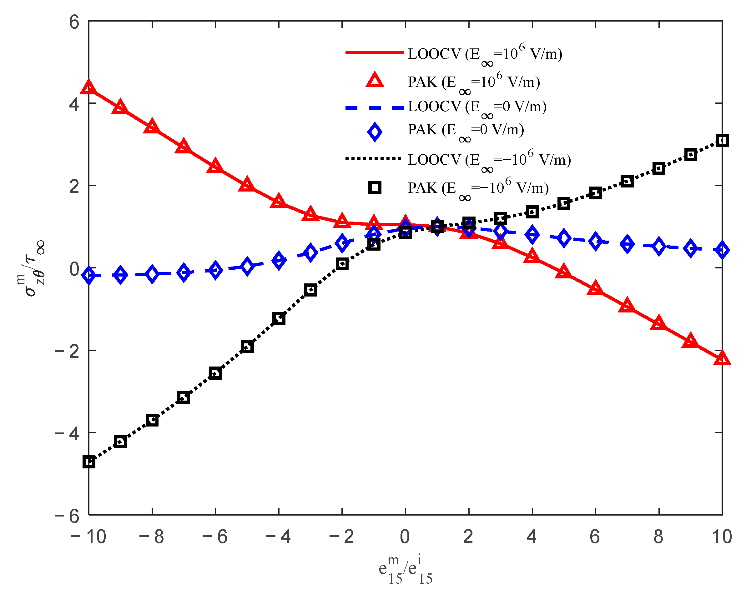
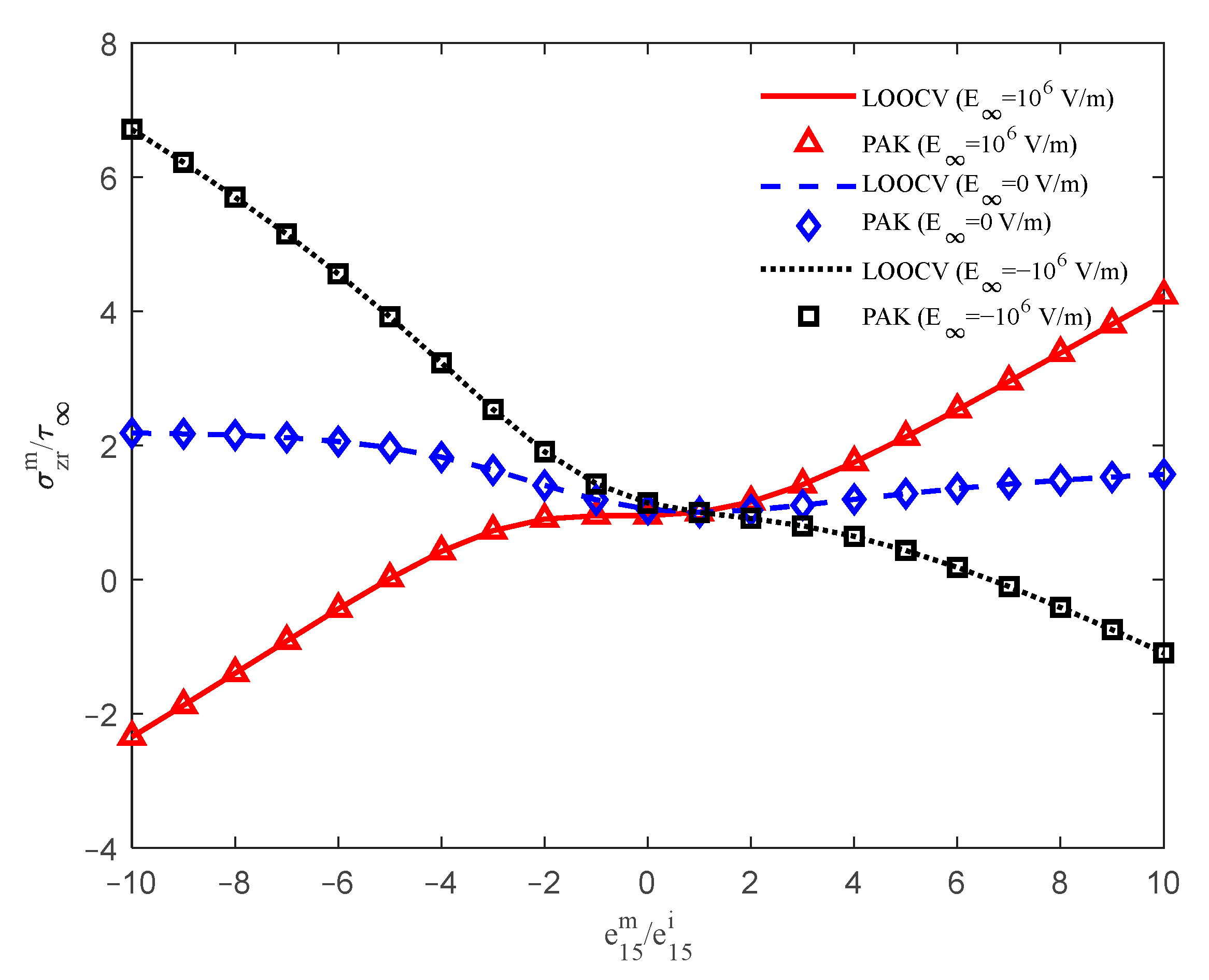
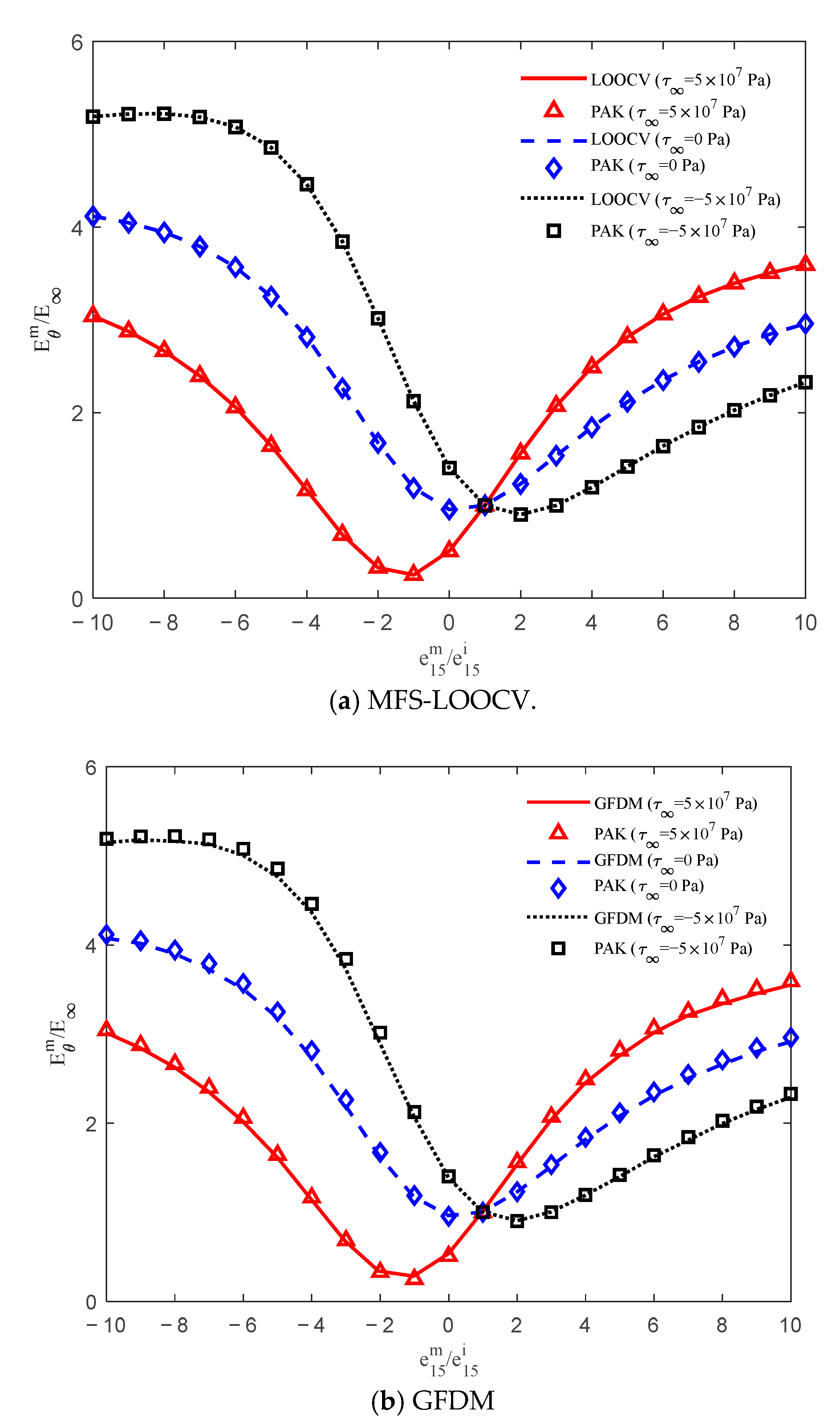
Consider a single circular piezoelectric inclusion embedded in a piezoelectric matrix, as shown in Figure 5. The material parameters are $e_{15}^i=10.0 {\mathrm{Cm}}^{-2}$, ${\epsilon }_{11}^m={\epsilon }_{11}^i=1.51\times {10}^{-8} {\mathrm{CV}}^{-1}{\mathrm{m}}^{-1}$ and $c_{44}^m=c_{44}^i=3.53\times {10}^{10} {\mathrm{Nm}}^{-2}$. The far-field antiplane shear and far-field in-plane electric field are ${\tau }_{\infty }=5\times {10}^7 {\mathrm{Nm}}^{-2}$ and $E_{\infty }={10}^6 \mathrm{V}/\mathrm{m}$, $E_{\infty }=0 \mathrm{V}/\mathrm{m}$, $E_{\infty }=-{10}^6 \mathrm{V}/\mathrm{m}$, respectively. The stress concentrations ${\sigma }_{z\theta }/{\tau }_{\infty }$ at $\left(r,0\right)$ and ${\sigma }_{zr}/{\tau }_{\infty }$ at $\left(0,r\right)$ versus different ratios of piezoelectric modulus are plotted in Figure 6 and Figure 7. Also, when $E_{\infty }={10}^6 \mathrm{V}/\mathrm{m}$, and ${\tau }_{\infty }=5\times {10}^7 {\mathrm{Nm}}^{-2}$, ${\tau }_{\infty }=0 {\mathrm{Nm}}^{-2}$, ${\tau }_{\infty }=5\times {10}^7 {\mathrm{Nm}}^{-2}$, the electric concentration $E_{\theta }/E_{\infty }$ at $\left(r,0\right)$ is shown in Figure 8 with different ratios of piezoelectric constants. In Figure 8, we also proposed the results by the generalized finite difference method (GFDM) to show the advantages of the proposed method. As shown in the figures, the maximum stress concentration and the maximum electric concentration occur when the poling direction is negative $e_{15}^m/e_{15}^i=-10$. The calculated results are in agreement with those of Pak [2].

The relative error is used to evaluate the stability and accuracy of the method. When the collocation points are randomly distributed, according to

Table 1. Relative error of normalized stress ${\sigma }_{zr}/{\tau }_{\infty }$ with a different number of collocation nodes.

nb	26	32	38	44	50
$e_{15}^m/e_{15}^i=-8$	1.30 × 10−3	2.43 × 10−4	4.52 × 10−5	8.36 × 10−6	1.54 × 10−6
$e_{15}^m/e_{15}^i=-6$	2.71 × 10−4	4.69 × 10−5	8.35 × 10−6	1.51 × 10−6	2.76 × 10−7
$e_{15}^m/e_{15}^i=6$	9.75 × 10−4	1.81 × 10−4	3.36 × 10−5	6.21 × 10−6	1.15 × 10−6
$e_{15}^m/e_{15}^i=8$	1.11 × 10−3	2.07 × 10−4	3.85 × 10−5	7.12 × 10−6	1.31 × 10−6

, with the increase in the number of points, the accuracy of calculation results can be improved. Furthermore, we introduced small perturbations to the boundary conditions to test the computational stability of the results shown in

Table 2. Relative error of normalized stress ${\sigma }_{zr}/{\tau }_{\infty }$ with different $\mathsf{\delta }$ on boundary conditions.

$\mathsf{\delta }$	0	0.1	0.01	0.001
$e_{15}^m/e_{15}^i=-10$	8.01 × 10−12	4.29 × 10−2	4.25 × 10−3	9.39 × 10−3
$e_{15}^m/e_{15}^i=4$	1.62 × 10−12	1.41 × 10−2	3.19 × 10−3	4.73 × 10−4
$e_{15}^m/e_{15}^i=8$	2.51 × 10−11	3.80 × 10−2	4.24 × 10−3	7.08 × 10−4
$e_{15}^m/e_{15}^i=10$	6.11 × 10−14	7.65 × 10−2	5.57 × 10−3	8.81 × 10−4

, where $\delta$ = 0, 0.1, 0.01, and 0.001 represent the magnitude of perturbation and the given boundary conditions are mixed by some noise

$$\overline{f}=f\left(1+\delta •\mathrm{rand}()\right)$$

where f is the original boundary condition, $\overline{f}$ is the boundary condition with perturbation, and rand is a function used to generate uniformly distributed random numbers in the interval (0,1).

3.2. Case 2: Two Circular Piezoelectric Inclusions

Consider two circular piezoelectric inclusions embedded in a piezoelectric matrix; in this case, two inclusions have different relative locations, distances, and sizes ($r_2=2r_1$).

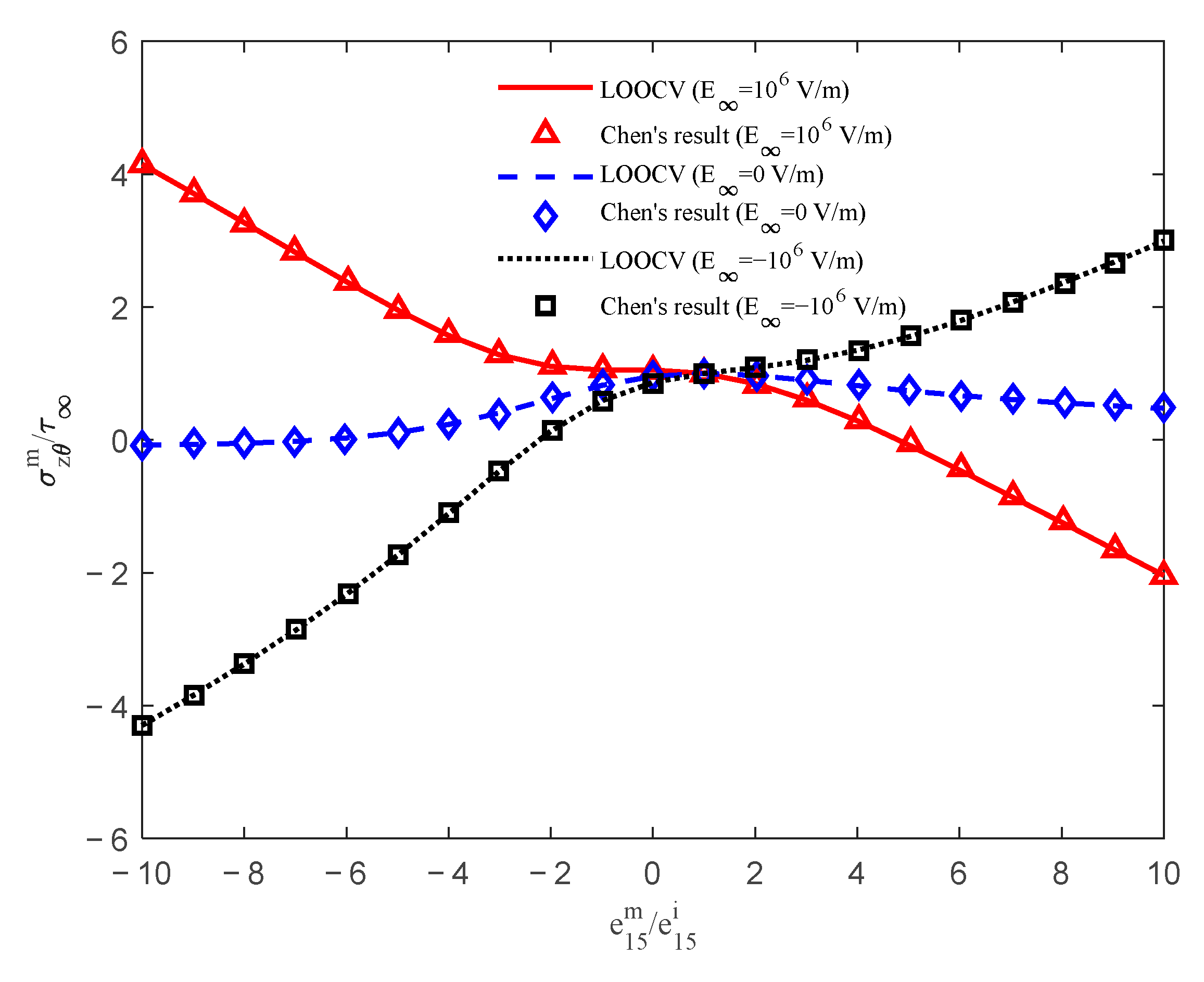
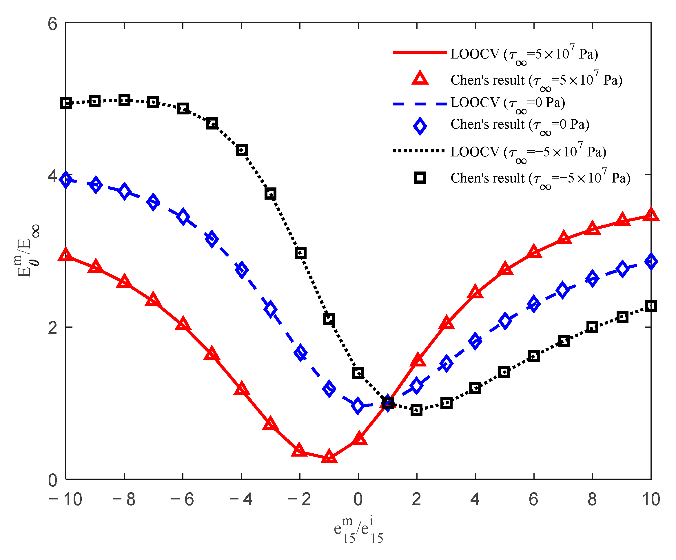
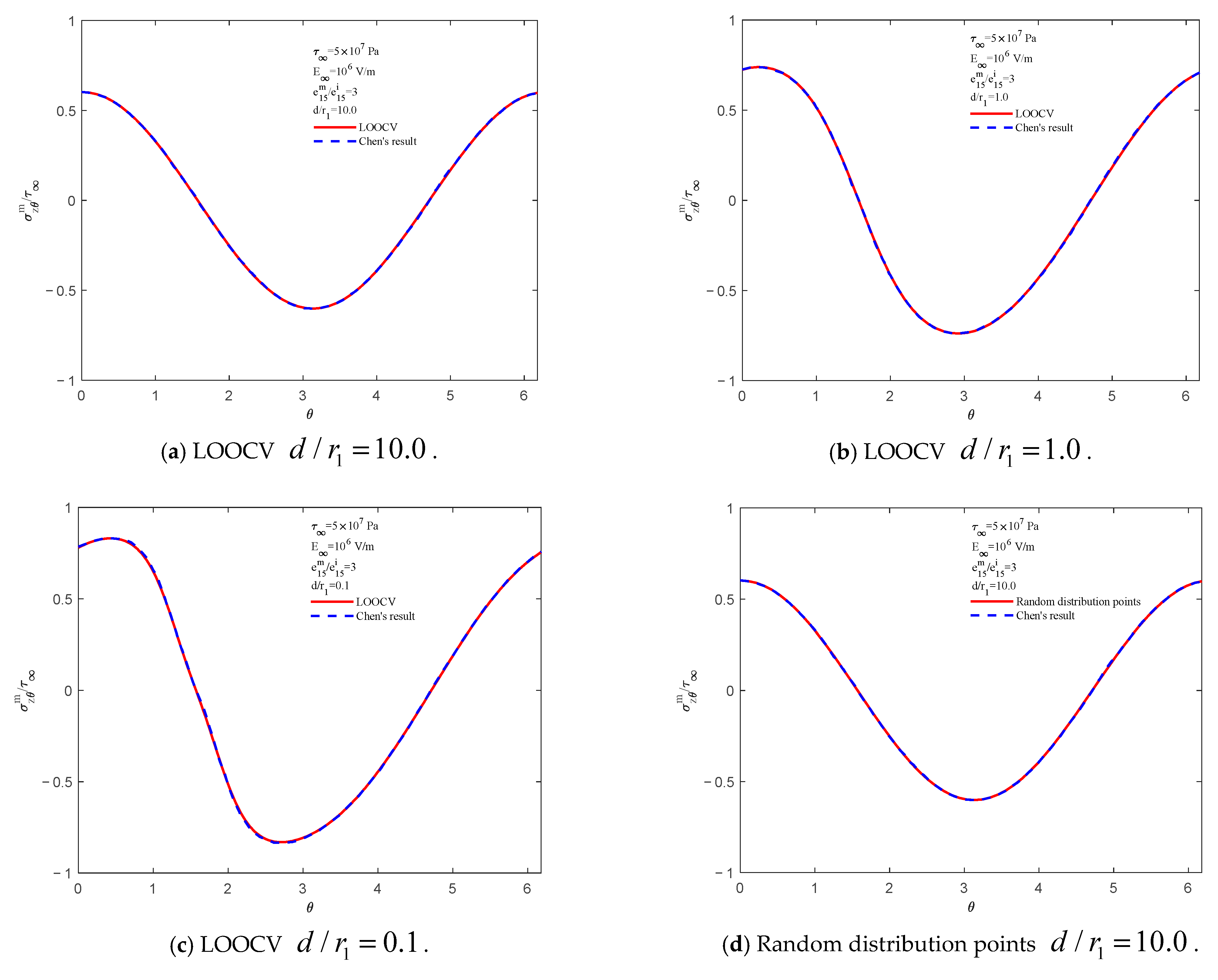
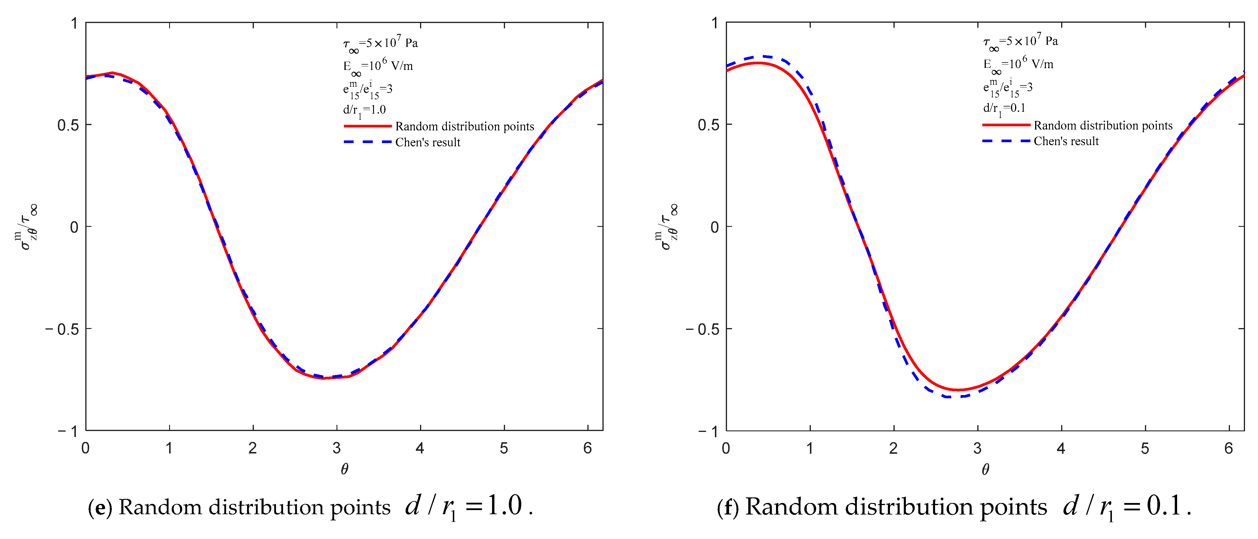
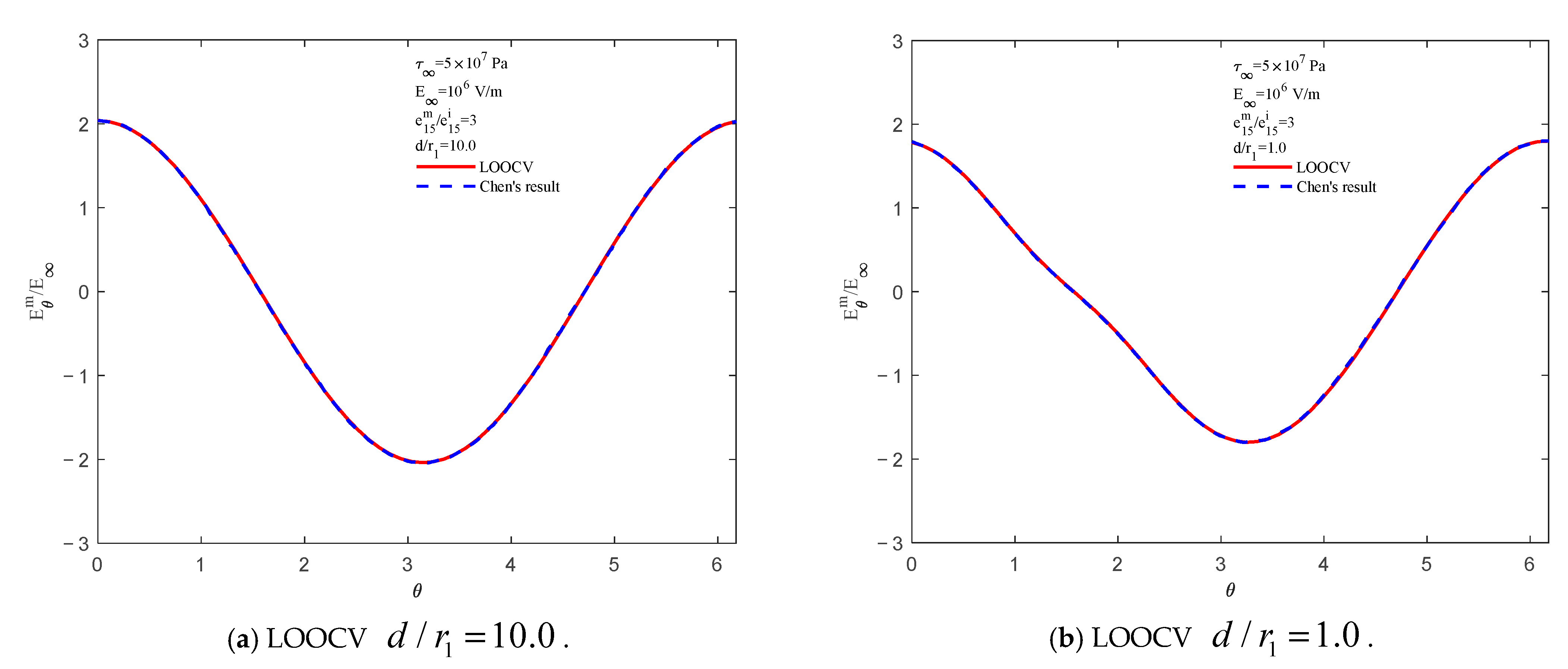
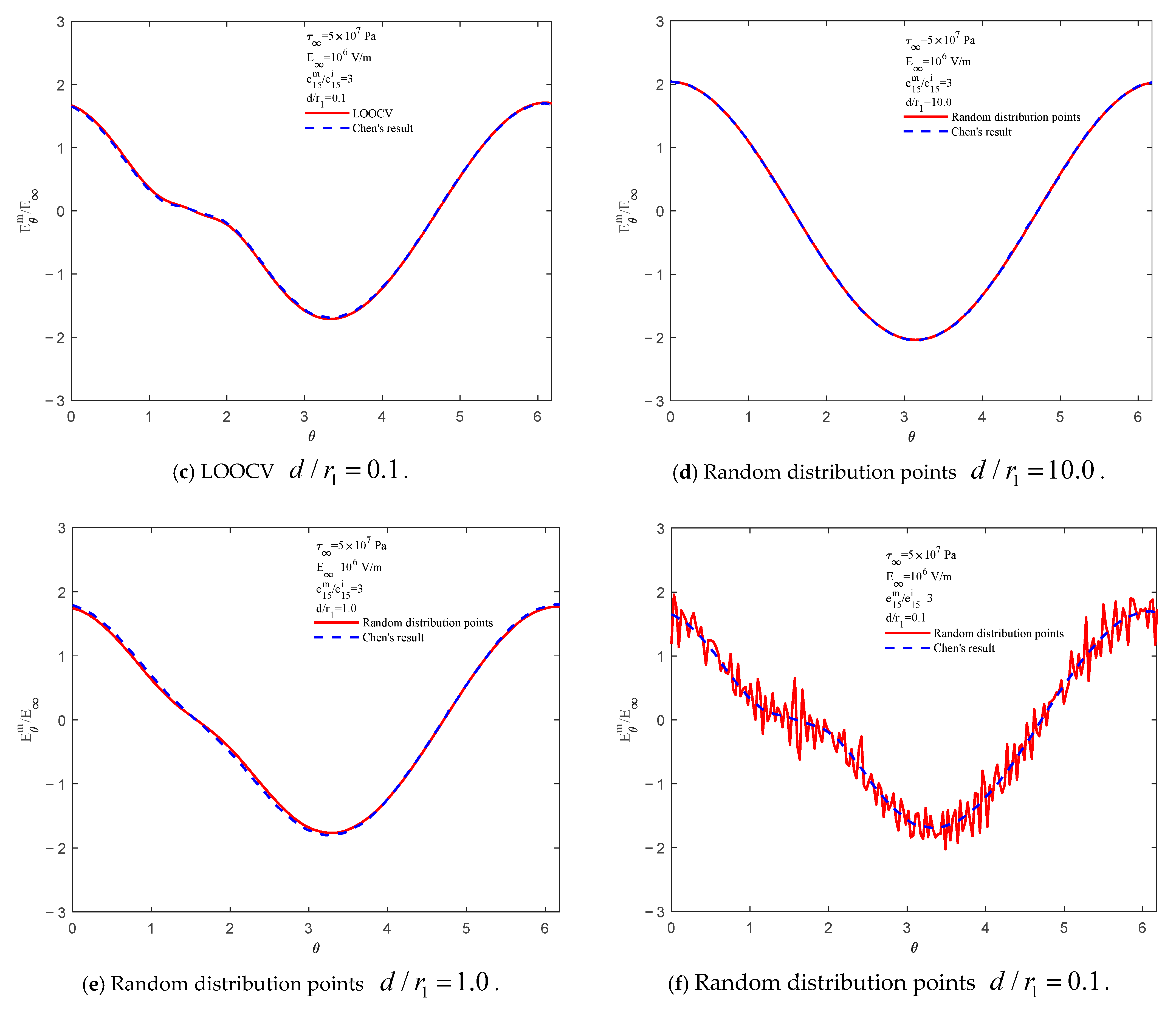
Two inclusions parallel to applied loadings, as shown in Figure 9. The material parameters are $e_{15}^i=10.0 {\mathrm{Cm}}^{-2}$, ${\epsilon }_{11}^m={\epsilon }_{11}^i=1.51\times {10}^{-8} {\mathrm{CV}}^{-1}{\mathrm{m}}^{-1}$, and $c_{44}^m=c_{44}^i=3.53\times {10}^{10} {\mathrm{Nm}}^{-2}$. Under the remote loadings ${\tau }_{\infty }=5\times {10}^7 {\mathrm{Nm}}^{-2}$ and $d/r_1=10.0$, the stress concentration ${\sigma }_{z\theta }/{\tau }_{\infty }$ at $\left(r_1,0\right)$ versus different ratios of piezoelectric modulus is plotted in Figure 10. When the remote loadings are $E_{\infty }={10}^6 \mathrm{V}/\mathrm{m}$ and $d/r_1=10.0$, the electric field concentration $E_{\theta }/E_{\infty }$ at $\left(r_1,0\right)$ versus different ratios of piezoelectric modulus is plotted in Figure 11. The results are similar to the solutions for a single inclusion in Figure 6 and Figure 8 because the two inclusions are far apart. When $c_{44}^m/c_{44}^i=3$, both the tangential stress ${\sigma }_{z\theta }$ and the tangential electric field $E_{\theta }$ in the matrix along the boundary of the small inclusion versus different ratios of $d/r_1$ are plotted in Figure 12 and Figure 13. The results are consistent with those of Chen [6]. When $d/r_1=10.0$ and $d/r_1=1.0$, the number of collocation points $nb=120$. Conversely, when $d/r_1=0.1$, the number of collocation points should increase suitably to avoid singularity, the number of collocation points $nb=400$. The numerical results of random distribution points provided in Figure 12 and Figure 13 are unsatisfactory. When the source points are randomly distributed, the number of conditions of the interpolation matrix may increase significantly, making the obtained result unstable. If the distance between the source point and the collocation point is too small or unevenly distributed, the matrix will be close to singular, and the small disturbance will be amplified when solving the linear system, which will affect the accuracy of the solution.

Two inclusions perpendicular to the applied loadings as shown in Figure 14, the material parameters are $e_{15}^i=10.0 {\mathrm{Cm}}^{-2}$, ${\epsilon }_{11}^m={\epsilon }_{11}^i=1.51\times {10}^{-8} {\mathrm{CV}}^{-1}{\mathrm{m}}^{-1}$ and $c_{44}^m=c_{44}^i=3.53\times {10}^{10} {\mathrm{Nm}}^{-2}$. The remote loadings are ${\tau }_{\infty }=5\times {10}^7 {\mathrm{Nm}}^{-2}$ and $E_{\infty }={10}^6 \mathrm{V}/\mathrm{m}$. The stress concentration ${\sigma }_{z\theta }/{\tau }_{\infty }$ of the different ratios of $d/r_1$ versus piezoelectric modulus ratio at $\left(r_1,0\right)$ is plotted in Figure 15. The results obtained are in good agreement with those of in [6]. The maximum stress concentration occurs when $d/r_1=0.1$; when two inclusions approach each other, the interaction between them is more significant, resulting in increased stress concentration. When $d/r_1=10.0$ and $d/r_1=1.0$, the number of collocation points $nb=120$. When $d/r_1=0.1$, to ensure accuracy, the number of collocation points increases $nb=800$.

3.3. Case 3: Single Elliptical Piezoelectric Inclusion

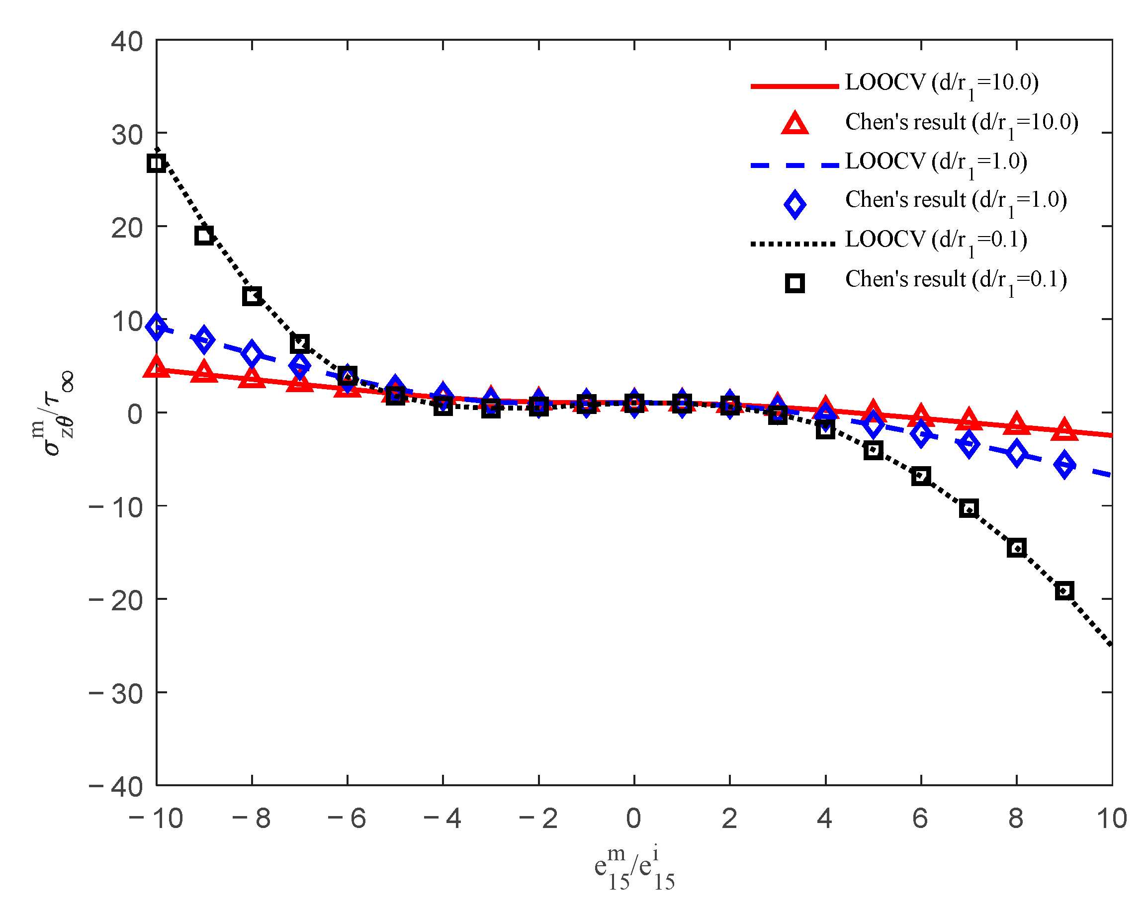
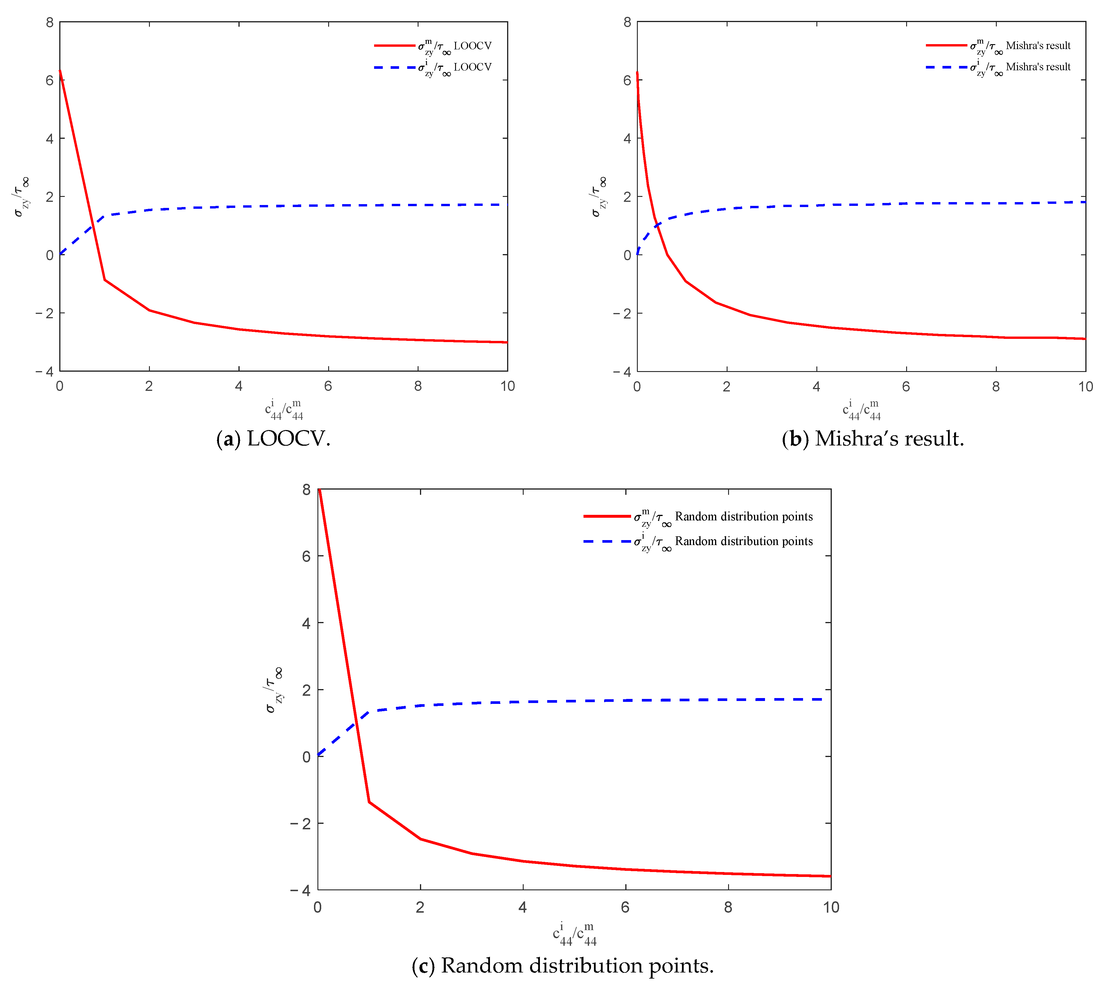
The single elliptical piezoelectric inclusion with a major and a minor semi-axis of $a$ and $b$ ($a/b=5$)embedded in a piezoelectric matrix is shown in Figure 16. The material parameters are $c_{44}^m=3.53\times {10}^{10} {\mathrm{Nm}}^{-2}$, $e_{15}^m=17.0 {\mathrm{Cm}}^{-2}$, ${\epsilon }_{11}^m=1.51\times {10}^{-8} {\mathrm{CV}}^{-1}{\mathrm{m}}^{-1}$. The remote loadings are ${\tau }_{\infty }={10}^8 {\mathrm{Nm}}^{-2}$ and $E_{\infty }={10}^6 \mathrm{V}/\mathrm{m}$. When the piezoelectric and dielectric modulus of the inclusion is $1/10$ of those in matrix ($e_{15}^i/e_{15}^m=1/10$, ${\epsilon }_{11}^i/{\epsilon }_{11}^m=1/10$), the stress concentration ${\sigma }_{zy}/{\tau }_{\infty }$ versus piezoelectric modulus ratio at $\left(a,0\right)$ is shown in Figure 17. The higher the ratio of elastic modulus $c_{44}^i/c_{44}^m$ means that the inclusion is harder than the matrix. When the inclusion becomes harder, the stress concentration becomes negative. The results agreed well with those of Mishra [10]. Meanwhile, the result using MFS through random distribution points is also provided, which indicates that the LOOCV algorithm is effective.

3.4. Case 4: Two Elliptical Piezoelectric Inclusions

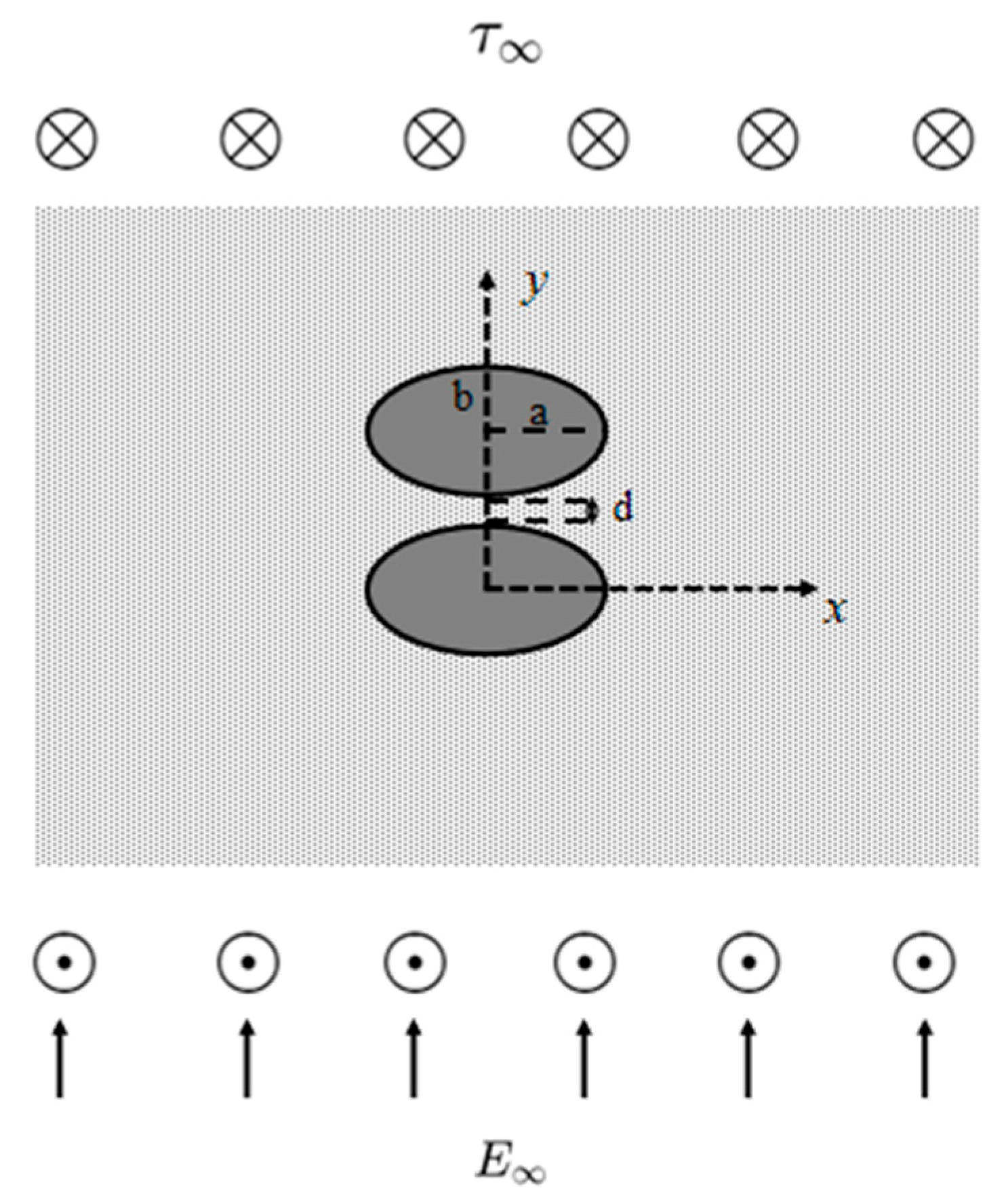
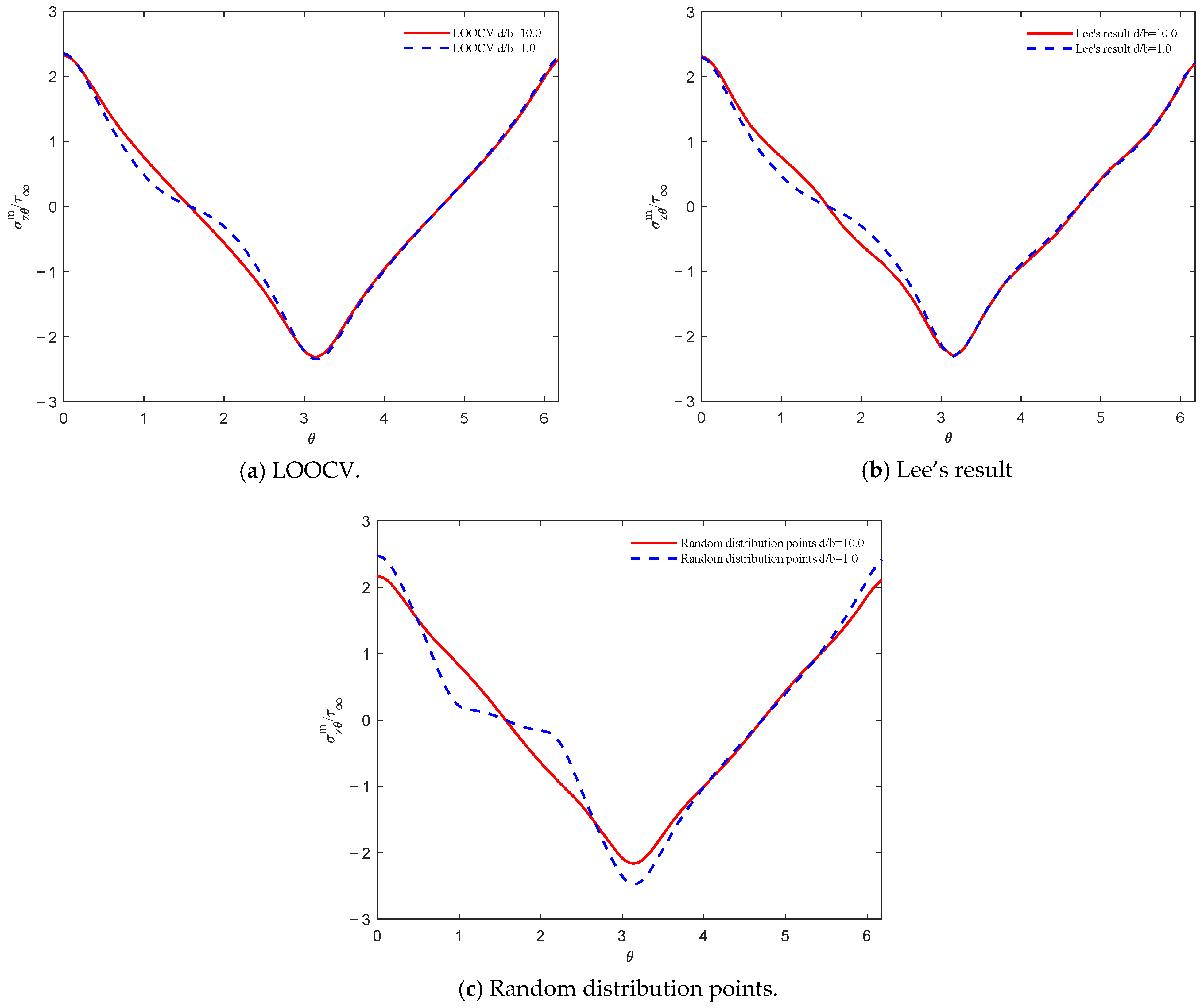
Two elliptical piezoelectric inclusions with a major and a minor semi-axis of $a$ and $b$ ($a/b=2$) embedded in a piezoelectric matrix are shown in Figure 18. The material parameters are the same as those in Section 3.2 and $e_{15}^m/e_{15}^i=-5$. The tangential stress ${\sigma }_{z\theta }$ in the matrix along the boundary of the nether inclusion versus different ratios of $d/b$ are plotted in Figure 19. The numerical results are basically identical to those of Lee [11].

4. Conclusions

From the foregoing numerical examples, the MFS without the LOOCV algorithm can obtain accurate results when calculating the boundaries of symmetry rules and single problems. In this case, the LOOCV algorithm can further improve the accuracy of the accurate results by several orders of magnitude. In more complicated cases, the interval in which the source point is placed becomes limited. Random placement of source points leads to errors. The LOOCV algorithm accurately selects the location of the source point and ensures the accuracy of the MFS. Even in the more complex, closer to the boundaries of defect shapes in engineering practice, the LOOCV algorithm also shows its high efficiency and applicability. Therefore, the proposed MFS, in combination with the LOOCV algorithm, is an accurate and stable meshless method for the solution of antiplane piezoelectricity problems with multiple inclusions. The comparison between different meshless methods is shown in

Table 3. Comparison between different meshless methods.

Meshless Method	Basis Function	Node Distribution	Method to Avoid Singularity	Strengths	Weakness
Method of fundamental solution [12]	Fundamental solution	Source nodes and collocation points	Source nodes are placed away from the boundary	High-dimensional complex geometry problems	Dense matrix
Regularized meshless method [7]	Double layer potentials	Boundary nodes only	Subtracting and adding-back technique	High accuracy	Difficult for irregular domain problems
Generalized finite difference method [8]	Taylor series	Nodes on the boundary and in the domain	No singularity	Sparse matrix	Sensitive to the placement of the nodes

, which better illustrates the characteristics of this method. It should be mentioned that we only consider the problems of simple geometries. The interpolation matrix is dense, so the calculation time and stability may become the bottleneck of this method in the calculation of large-scale problems. In subsequent research, we will further investigate localization techniques for the meshless method. Then, the proposed algorithm can be used in various real applications, such as the design of sensors and actuators, which will be discussed later.

References

- Bleustein, J.L. A new surface wave in piezoelectric materials. Appl. Phys. Lett. 1968, 13, 412–413. [Google Scholar] [CrossRef]
- Pak, Y.E. Circular inclusion problem in antiplane piezoelectricity. Int. J. Solids Struct. 1992, 29, 2403–2419. [Google Scholar] [CrossRef]
- Honein, T.; Honein, B.V.; Honein, E.; Herrmann, G. On the interaction of two piezoelectric fibers embedded in an intelligent material. J. Intell. Mater. Syst. Struct. 1995, 6, 229–236. [Google Scholar] [CrossRef]
- Chao, C.K.; Chang, K.J. Interacting circular inclusions in antiplanepiezoelectricity. Int. J. Solids Struct. 1999, 36, 3349–3373. [Google Scholar] [CrossRef]
- Wu, L.; Chen, J.; Meng, Q. Two piezoelectric circular cylindrical inclusions in the infinite piezoelectric medium. Int. J. Eng. Sci. 2000, 38, 879–892. [Google Scholar] [CrossRef]
- Chen, J.T.; Wu, A.C. Null-field approach for piezoelectricity problems with arbitrary circular inclusions. Eng. Anal. Bound. Elem. 2006, 30, 971–993. [Google Scholar] [CrossRef]
- Chen, K.H.; Kao, J.H.; Chen, J.T. Regularized meshless method for antiplane piezoelectricity problems with multiple inclusions. Comput. Mater. Contin. 2009, 9, 253. [Google Scholar]
- Yu, H.; Lin, J. Simulation of antiplane piezoelectricity problems with multiple inclusions using the generalized finite difference method. Eur. J. Mech.-A/Solids 2022, 94, 104615. [Google Scholar] [CrossRef]
- Pak, Y.E. Elliptical inclusion problem in antiplane piezoelectricity: Implications for fracture mechanics. Int. J. Eng. Sci. 2010, 48, 209–222. [Google Scholar] [CrossRef]
- Mishra, D.; Park, C.Y.; Yoo, S.H.; Pak, Y.E. Closed-form solution for elliptical inclusion problem in antiplane piezoelectricity with far-field loading at an arbitrary angle. Eur. J. Mech.-A/Solids 2013, 40, 186–197. [Google Scholar] [CrossRef]
- Lee, Y.T.; Chen, J.T.; Kuo, S.R. Null-field integral approach for the piezoelectricity problems with multiple elliptical inhomogeneities. Eng. Anal. Bound. Elem. 2014, 39, 111–120. [Google Scholar] [CrossRef]
- Kupradze, V.D.; Aleksidze, M.A. The method of functional equations for the approximate solution of certain boundary value problems. USSR Comput. Math. Math. Phys. 1964, 4, 82–126. [Google Scholar] [CrossRef]
- Liu, C.S.; Kuo, C.L. Pseudo and anisotropic MFS for Laplace equation and optimal sources using maximal projection method with a substitution function. Eng. Anal. Bound. Elem. 2024, 158, 313–320. [Google Scholar] [CrossRef]
- Grabski, J.K. On the sources placement in the method of fundamental solutions for time-dependent heat conduction problems. Comput. Math. Appl. 2021, 88, 33–51. [Google Scholar] [CrossRef]
- Grabski, J.K.; Mrozek, A. Identification of elastoplastic properties of rods from torsion test using meshless methods and a metaheuristic. Comput. Math. Appl. 2021, 92, 149–158. [Google Scholar] [CrossRef]
- Ling, L.; Schaback, R. An improved subspace selection algorithm for meshless collocation methods. Int. J. Numer. Methods Eng. 2009, 80, 1623–1639. [Google Scholar] [CrossRef]
- Tsai, C.C.; Lin, Y.C.; Young, D.L.; Atluri, S.N. Investigations on the accuracy and condition number for the method of fundamental solutions. Comput. Model. Eng. Sci. 2006, 16, 103. [Google Scholar]
- Liu, C.S. An equilibrated method of fundamental solutions to choose the best source points for the Laplace equation. Eng. Anal. Bound. Elem. 2012, 36, 1235–1245. [Google Scholar] [CrossRef]
- Wang, F.; Liu, C.S.; Qu, W. Optimal sources in the MFS by minimizing a new merit function: Energy gap functional. Appl. Math. Lett. 2018, 86, 229–235. [Google Scholar] [CrossRef]
- Lin, S.R.; Young, D.L.; Chen, C.S. Ghost-point based radial basis function collocation methods with variable shape parameters. Eng. Anal. Bound. Elem. 2021, 130, 40–48. [Google Scholar] [CrossRef]
- Zhang, L.P.; Li, Z.C.; Huang, H.T.; Lee, M.G. New locations of source nodes for method of fundamental solutions solving Laplaces equation; pseudo radial-lines. Eng. Anal. Bound. Elem. 2022, 136, 93–115. [Google Scholar] [CrossRef]
- Chen, C.S.; Noorizadegan, A.; Young, D.L.; Chen, C.S. On the selection of a better radial basis function and its shape parameter in interpolation problems. Appl. Math. Comput. 2023, 442, 127713. [Google Scholar] [CrossRef]
- Rippa, S. An algorithm for selecting a good value for the parameter c in radial basis function interpolation. Adv. Comput. Math. 1999, 11, 193–210. [Google Scholar] [CrossRef]
- Fasshauer, G.E.; Zhang, J.G. On choosing optimal shape parameters for RBF approximation. Numer. Algorithms 2007, 45, 345–368. [Google Scholar] [CrossRef]
- Chen, C.S.; Karageorghis, A.; Li, Y. On choosing the location of the sources in the MFS. Numer. Algorithms 2016, 72, 107–130. [Google Scholar] [CrossRef]
Disclaimer/Publisher’s Note: The statements, opinions and data contained in all publications are solely those of the individual author(s) and contributor(s) and not of MDPI and/or the editor(s). MDPI and/or the editor(s) disclaim responsibility for any injury to people or property resulting from any ideas, methods, instructions or products referred to in the content. |
© 2025 by the authors. Licensee MDPI, Basel, Switzerland. This article is an open access article distributed under the terms and conditions of the Creative Commons Attribution (CC BY) license (https://creativecommons.org/licenses/by/4.0/).