Abstract
In this study, we propose a generalized framework based on the Simple Equations Method (SEsM) for finding exact solutions to systems of fractional nonlinear partial differential equations (FNPDEs). The key developments over the original SEsM in the proposed analytical framework include the following: (1) an extension of the original SEsM by constructing the solutions of the studied FNPDEs as complex composite functions which combine two single composite functions, comprising the power series of the solutions of two simple equations or two special functions with different independent variables (different wave coordinates); (2) an extension of the scope of fractional wave transformations used to reduce the studied FNPDEs to different types of ODEs, depending on the physical nature of the studied FNPDEs and the type of selected simple equations. One variant of the proposed generalized SEsM is applied to a mathematical generalization inspired by the classical Boussinesq model. The studied time-fractional Boussinesq-like system describes more intricate or multiphase environments, where classical assumptions (such as constant wave speed and energy conservation) are no longer applicable. Based on the applied SEsM variant, we assume that each system variable in the studied model supports multi-wave dynamics, which involves combined propagation of two distinct waves traveling at different wave speeds. As a result, numerous new multi-wave solutions including combinations of different hyperbolic, elliptic, and trigonometric functions are derived. To visualize the wave dynamics and validate the theoretical results, some of the obtained analytical solutions are numerically simulated. The new analytical solutions obtained in this study can contribute to the prediction and control of more specific physical processes, including diffusion in porous media, nanofluid dynamics, ocean current modeling, multiphase fluid dynamics, as well as several geophysical phenomena.
Keywords:
extended simple equation method; time-fractional Boussinesq-like system; analytical solutions; numerical simulations MSC:
35A24; 35G50
1. Introduction
Over the past two decades, the fractional nonlinear partial differential equations (FNPPDEs) have gained considerable popularity in the scientific community for modeling and analyzing a wide range of phenomena observed in the real world. This efficient framework allows for more accurately reproducing the complex wave dynamics of model systems encountered in diverse fields such as biology and ecology [1,2,3], fluid dynamics [4,5,6,7], finance and economics [8,9,10], engineering [11,12,13], among others. These systems often exhibit features such as memory effects, spatial heterogeneity, and nonlocal interactions that integer-order models fail to adequately address. One approach to better understand this unconventional dynamic behavior is to find analytical solutions to the such models and their expert analysis. Finding exact solutions to FNPDEs, unlike those of NPDEs, is more difficult due to the necessary combination of elements from nonlinear dynamics with those arising from the fractional derivative’s order.
To date, two main approaches to finding exact and approximate analytical solutions of FNPDEs dominate the scientific literature: (1) Using fractional transformations allow for reducing the studied NFPDEs to integer order nonlinear ODEs. Then, various well-known approaches from the ODE theory can be applied to the latter to obtain exact general and particular solutions of NPDEs. The most famous and applied methodologies in this direction use the so-called ansatz techniques [14]. Based on ansatz techniques, numerous analytical methods have been developed, including the Hirota method [15], the homogeneous balance method [16], the auxiliary equation method [17], the Jacobi elliptic function expansion method [18], the (G′/G)-expansion method [19], the F-expansion method [20], the tanth-function method [21], the first integral method [22], the exponential function method [23], the simplest equation method [24], the modified method of simplest equation [25,26,27], etc. There are also numerous studies that apply these methods to find analytical solutions to various single NPDEs and systems of NPDEs. The SEsM, used in this study, is a relatively new methodology [28,29]. It is an extension of the modified method of simple equation and has an almost universal nature. This is because most of the above-mentioned methods in this category are particular cases, as proven in [30,31,32,33]. (2) Using standard traveling wave transformations allow for reducing the studied FNPDEs to simpler fractional PDEs or fractional ODEs, of which the corresponding analytical solutions are known (for instance, see Ref. [34]). Then, similarly to the first approach, analytical solutions of the studied FNPDEs are constructed on the basis of known analytical solutions of fractional ODEs. Among the methods in this category, the most widely used is so called fractional sub-equation method [35,36,37,38]. This method is based on known solutions of the fractional ODE of Riccati and its sub-variants. Another popular method in this category is the fractional elliptic Jacobi equation method [39,40], which uses Jacobi elliptic functions to derive analytical solutions of the studied FPDEs. When using the second approach, the Mittag–Leffler functions often appear in solutions of the studied FNPDEs, because they effectively describe the behavior of systems with fractional order.
In this study, we propose a generalized SEsM algorithm for finding exact solutions to systems of FNPDEs (or single FNPDEs), which encompasses both approaches presented above. It is fundamentally based on the SEsM algorithm for finding exact solutions to integer-order NPDEs proposed in [41,42,43,44]. According to the original SEsM algorithm [41,42,43,44], the solutions of the studied integer-order NPDEs are presented as complex composite functions, including series of solutions of two (or more) simple equations or two (or more) special functions. One of our main contributions to the SEsM [41,42,43,44] is that we extend the range of constructed solutions assuming that the simple equations used have different independent variables. The latter is a new approach that was first applied to find analytical solutions of the extended integer-order KDV equation in a co-authored paper [45]. Numerous traveling wave solutions have been derived in [45] using an ODE of Abel, an ODE of Bernoulli, an ODE of Riccati, and its sub-variants. Later, in [46], the authors independently proposed a similar methodology based on the extended Kudryashov method, as it was applied to find exact solutions of an integer-order Boussinesq-like system and the integer-order shallow-water wave equation. To obtain exact analytical solutions of the aforementioned models, the authors in [46] used two sub-variants of the ODE of Riccati as simple equations. Another novel aspect of the proposed SEsM algorithm in this study is its adaptation to find exact solutions to FNPDEs by proposing the introduction of different types of fractional transformations depending on the fractional derivatives chosen to study FNPDEs and the type of simple equations used to extract their solutions. In terms of finding exact solutions to systems of FNPDEs, a similar version of the extended SEsM proposed in this paper was applied in [47,48] to dynamical models describing natural processes in fluid mechanics and ecology. In these studies, the obtained traveling wave solutions were presented by sums of two single composite functions containing the solutions of two distinct simple equations with the same independent variable. In [49,50], another version of the extended SEsM was applied to an extended variant of a popular ecological system of FNPDEs. In these studies, the obtained analytical solutions of the studied system are presented by distinct single composite functions with different independent variables (different wave coordinates) for each system variable. In this study, we modify and extend the SEsM algorithm, proposed in [47,48], as explained above. Our aim is to show the capabilities provided by the generalized SEsM algorithm presented below for finding exact solutions to systems of FNPDEs that describe the complex wave behavior of real-world processes.
Below, we demonstrate an application of the generalized SEsM algorithm to a specific system of FNPDEs, including only one of its variant, which is connected to the first approach above given. Let us consider a system of time-fractional NPDEs of a Boussinesq-like kind [51].
where is a time-fractional number and k is an arbitrary coefficient. In fact, Equation (1) can be treated as a mathematical generalization inspired by the classical Boussinesq model, but not intended as a direct physical hydrodynamic model in the conventional sense. It is well known that the classical Boussinesq system has a clear hydrodynamical origin, describing long waves in shallow water, and it is derived from fundamental physical laws under specific assumptions. Introducing a fractional time derivative in this system obscures the classical physical interpretation, as the fractional operator accounts for memory effects and anomalous dispersion absent in the traditional shallow water model. However, this does not sever its hydrodynamic connection, i.e., the fractional extensions are used to model more complex real systems, including interactions with porous media, sediments, and complex boundaries. In this way, Equation (1) can be considered as a generalized hydrodynamical model for more intricate or multiphase environments, where classical assumptions (such as constant wave speed and energy conservatism) are no longer applicable. In addition, in the classical case (when = 1), the system (1) has a purely hyperbolic structure, i.e., waves propagate at a constant speed, and energy is conserved. When in Equation (1), however, the fractional time derivative introduces memory effects, leading to wave speed variations, i.e., slower propagation for < 1 (sub-diffusive behavior) or faster propagation for > 1 (super-diffusive behavior). Fractional relaxation also causes energy dissipation, modeling real-world losses. Additionally, in many cases, the system can become temporally nonlocal, meaning the future state depends on its entire past, similar to sedimentary layers. These effects result in complex, non-classical wave behaviors, including accelerating, decaying, or anomalous dispersive waves. While the dynamical behavior of the classical Boussinesq system has been extensively studied over the years, the wave anomalies arising from the introduction of a fractional derivative in it remain not fully understood. In this sense, one of our motivations of this study is to clarify some of these new features in Equation (1) by extracting its analytical solutions.
On the basis of the extended SEsM algorithm provided below, we search for analytical solutions of Equation (1) in a more specific manner, taking into account its specific dynamical characteristics explained above. First of all, we consider Equation (1) in terms of the modified fractional Riemann–Liouville derivative. In our opinion, it provides a more physically realistic description of wave evolution in real media, since it provides better consistency with measurable initial conditions and reflects memory effects typical of complex multiphase interactions. The modified fractional Riemann–Liouville derivative also allows for a more flexible treatment of dissipative and anomalous dispersion effects encountered in real physical processes. Secondly, given that, in Equation (1), the wave propagation is no longer uniform, with speeds varying due to memory effects and energy dissipation, it is natural to consider solutions that account for this complexity. In this sense, we present the analytical solution of each variable in Equation (1) as a combination of solutions of two simpler equations with different independent variables (different wave coordinates). This approach allows us to capture the multi-speed nature of wave propagation in the system (1), reflecting sub-diffusive or super-diffusive effects, as well as nonlocal interactions that influence the system’s evolution over time. We hope that such a presentation of the aforementioned solutions provides more an accurate and insightful depiction of the complex behaviors inherent in the studied mathematical model.
2. Preliminaries
In this section, we present several important definitions of the modified Riemann–Liouville derivatives that we will use in the current study. These definitions are stated according to the basic results obtained by G. Jumarie in [52,53,54].
2.1. Fractional Derivative via Fractional Difference
Definition 1.
Let denote a continuous (but not necessarily differentiable) function, and let denote a constant discretization span. Define the forward operator by the equality (the symbol means that the left side is defined by the right side).
then the fractional difference of order α, , of is defined by the expression
and its fractional derivative of order α is defined by the limit
2.2. Modified Fractional Riemann–Liouville Derivative
Definition 2.
Refer to the function of Definition 1.
- (i) Assume that is a constant K. Then, its fractional derivative of order α is(ii) When is not a constant, we will setand its fractional derivative will be defined by the expressionin which, for negative α, one haswhilst for positive α, we will setWhen ,In order to find the fractional derivative of compound functions, the following equation holds:
2.3. Taylor’s Series of Fractional Order
Definition 3.
The continuous function has a fractional derivative of order . For any positive integer k and for any α, , the following equality holds:
where .
Definition 4.
If , then
or, if , then
3. Description of the Generalized SEsM Algorithm
In this section, we present the generalized algorithm of a specific version of SEsM, exposing all the possibilities it provides for obtaining various complex analytical solutions to systems of FNPDEs (or single FNPDEs), depending on the selected fractional transformation and simple equation’s types used by the implementer. As it is demonstrated below, unlike the original SEsM algorithm outlined in [41,42,43], we have swapped its first and second steps, incorporating methodological extensions into both steps of the original SEsM algorithm. In addition, the proposed SEsM algorithm presented below covers both approaches to the chosen traveling wave transformation discussed earlier in the paper. Our goal is to allow the user to choose which of the two approaches to use when extracting exact solutions to systems of FNPDEs similar to Equation (1).
Taking into account the problem we set out to solve in this study, we demonstrate all the possible steps of the above-mentioned algorithm for a system of two NPPDEs with two independent variables:
where D denotes the arbitrary fractional order derivative operator, as superscripts give its fractional number and subscripts denote time and partial derivatives. Here, and are polynomials of u and v and their derivatives, respectively, where and are unknown functions.
Remark 1.
We note that the variant of SEsM presented below is suitable to be applied mainly to real-world dynamical models of the type (15), where the system variables are expected to exhibit complex synchronized multi-layered wave behavior.
The generalized extended SEsM algorithm that is adopted for finding exact solutions of FNPDEs includes the following basic steps:
- Construction of the solutions of Equation (15). The solution of Equation (15) can be constructed as a complex composite function of two or more single-composite functions, involving solutions of two or more simple equations with different independent variables. There are many variants of combination between the single-composite function in constructing the corresponding solution, but below we will present only a few of its simplest forms:
- Variant 1:Variant 2:Variant 3:wherewhere and are solutions of simple equations, which are presented in Step 3 of the SEsM algorithm.
- 2.
- Selection of the traveling-wave-type transformation. To apply the SEsM to Equation (15), it is crucial to define the fractional derivatives in those equations. The choice of fractional derivatives (e.g., Riemann–Liouville, Caputo, conformable, etc.) is essential for accurately modeling wave dynamics and reflecting the system’s physical properties, based on factors like the process nature, boundary conditions, and memory effect interpretation. In this context, the following variants of transformations are possible:
- Variant 1: Use a fractional transformation. The choice of an explicit form of the fractional traveling wave transformation depends on how the fractional derivatives in Equation (15) are defined. Below, the most used fractional traveling wave transformations are selected:− Conformable fractional traveling wave transformation: , defined for conformable fractional derivatives [55];− Fractional complex transform: , defined for modified Riemann–Liouville fractional derivatives [52], which can applied for Caputo fractional derivatives and other fractional derivative types in studied FNPDEs [56].In the both cases, the studied FNPDEs are reduced to integer-order nonlinear ODEs.
- Variant 2: Use a standard traveling wave transformation. In this case, by introducing a traveling wave ansatz in the selected variant solutions from Step 1, the studied FNPDEs are reduced to fractional nonlinear ODEs.
- 3.
- Selection of the forms of the used simple equations.
- For Variant 1 of Step 2: The general form of the integer-order simple equations used is expressed as follows:By fixing and (at ) in Equation (20), different types of integer-order ODEs can be used as simple equations, such as the following:− ODEs of first order with known analytical solutions (for example, an ODE of Riccati, an ODE of Bernoulli, an ODE of Abel of first kind, an ODE of tanh-function, etc.);− ODEs of second order with known analytical solutions (for example, elliptic equations of Jaccobi and Weiershtrass and their sub-variants, an ODE of Abel of second kind, etc.). This scenario can be applied to specific classes FNPDEs (or NPDEs) (for instance, see [57]).
- For Variant 2 of Step 2: The general form of the fractional simple equations used is expressed as follows:By fixing and in Equation (21), different types of fractional ODEs can be used as simple equations, such as the fractional ODE of Riccati, the fractional ODE of Bernoulli, or other polynomial or elliptic form equations, of which solutions are available in the literature.
- 4.
- Derivation of the balance equations and the system of algebraic equations. The fixation of the explicit form of solutions of Equation (15) presented in Step 1 of the SEsM algorithm depends on the balance equations derived. Substitutions of the selected variants from Steps 1, 2, and 3 in Equation (15) leads to obtaining polynomials of the functions and . The coefficients in front of these functions include the coefficients of the solution of the considered FNPDEs as well as the coefficients of the simple equations used. Analytical solutions of Equation (15) can be extracted only if each coefficient in front of the functions and contains almost two terms. Equating these coefficients to zero leads to the formation of a system of nonlinear algebraic equations for each variant chosen according Steps 1, 2, and 3 of the SEsM algorithm.
- 5.
- Derivation of the analytical solutions. Any non-trivial solution of the above-mentioned algebraic system leads to a solution of the studied FNPDEs by replacing the specific coefficients in the corresponding variant solutions, given in Step 1 as well as by changing the traveling wave coordinates chosen by the variants given in Step 2. For simplicity, these solutions are expressed through special functions. For Variant 1 of Step 3, these special functions are and , as their explicit forms are determined on the basis of the specific form of the simple equations chosen (for reference, see Equation (20)). For Variant 2 of Step 3, the special functions are and , with exact forms that are determined by the type of fractional simple equations used (for reference, see Equation (21)).
- In this study, we demonstrate only some of the possibilities provided by the generalized SEsM algorithm, presented above, by applying only one of its variants to Equation (1).
4. Exact Solutions of the Time-Fractional Boussinesq-like System Using a Fractional Wave Transformation
According to the generalized SEsM algorithm, presented above, we choose to present the general solution of Equation (1) using Equation (16) as follows:
In view of the studied shallow water problem, we choose to present the memory effects occurring in the system (1) in the sense of modified Riemann–Liouville fractional derivatives, presented in Section 2. Thus, the fractional transformations take the following form:
In the simple equations (20), we choose to fix , and . Then, Equation (20) is reduced to
The balance equations are and . The substitution of Equations (22)–(24) in Equation (1) leads to a system of nonlinear equations. There are many variants and sub-variants of Equation (24) depending on the numerical values of their coefficients. For each of these variants or sub-variants, there are specific solutions, which are available in the literature. Below, we present only a few examples of specific sub-variants of simple equations of the (24) type. For example, as a starting point, we choose to use the first simple equation of Equation (24) in its complete form with respect to the coefficients , i.e., . Regarding the second simple equation of (24), however, we choose to use its simplest sub-variant, where . Then, the system of nonlinear algebraic equations is expressed as follows:
In the rest of this article, we present only a part of off-beat possible solutions which can be derived depending on the numerical values of the coefficients in the polynomial parts of Equation (24) for this specific case.
4.1. Case 1: When and in Equation (24)
Let us consider the case, where and in Equation (24). Then, Equation (24) is reduced to
We present the general solution of Equation (1) using special functions in the following manner:
For this specific case, several families of solutions of Equation (1) can be obtained depending on the numerical values of the coefficients and .
4.1.1. Variant 1: When and in Equation (26)
Let us consider the case, where and in Equation (26). Then, Equation (27) reduces to
where the special function is a particular solution of an ODE of second order, given in [57,58], and the special function presents particular solutions of an ODE of the second order, which can be found in [59].
We solve the algebraic system (25) by fixing . Many solutions of the system (25) can be derived, but we aim to find those solutions, where the coefficients are free parameters. This way, one non-trivial solution of this system is expressed as follows:
According to all possible variant solutions , the following families of solutions (28) of Equation (1) are possible:
where [57]
and [59]
In Equation (32), and are arbitrary constants.
where is presented in Equation (31) and [59]
In Equation (34), and are arbitrary constants.
where is presented in Equation (31) and [59]
In Equation (36), and are arbitrary constants. In all of the solutions provided in this subsection, and are expressed by Equation (23).
4.1.2. Variant 2: When and in Equation (26)
4.1.3. Variant 3: When and in Equation (26)
4.2. Case 2: When and in Equation (24)
Let us consider the case, where and in Equation (24). Then, Equation (24) is reduced to
We present the general solution of Equation (1) by special functions in the following manner:
In Equation (44), we choose to express the special function (the solutions of the first equation in (43)), in terms of Weierstrass-elliptic functions and [61]. The special function presents the same solutions, as those given in the previous section. Depending on variant solutions and , various families of solutions of Equation (1) can be selected.
4.2.1. Variant 1. When and in Equation (43)
One non-trivial solution of the algebraic system (25) at and , including the coefficients and as free parameters, is expressed as follows:
Then, the substitution of Equation (45) in Equation (44) leads to the following solutions of Equation (1):
where
and is presented in Equation (32).
where is presented in Equation (47) and is presented in Equation (34).
where is presented in Equation (47) and is presented in Equation (36).
where
and is presented in Equation (32).
where is presented in Equation (51) and is presented in Equation (34).
where is presented in Equation (51) and is presented in Equation (36).
where
and is presented in Equation (32).
where is presented in Equation (55) and is presented in Equation (34).
where is presented in Equation (55) and is presented in Equation (36).
where
and is presented in Equation (32).
where is presented in Equation (59) and is presented in Equation (34).
where is presented in Equation (59) and is presented in Equation (36).
where
and is presented in Equation (32).
where is presented in Equation (63) and is presented in Equation (34).
where is presented in Equation (63) and is presented in Equation (36).
where
and is presented in Equation (32).
where is presented in Equation (67) and is presented in Equation (34).
where is presented in Equation (67) and is presented in Equation (36). In all the solutions, presented in this subsection, and are expressed by Equation (23).
4.2.2. Variant 2: When and in Equation (43)
When , Equation (45) is reduced to the following:
The substitution of Equation (70) in the particular variant of Equation (44) leads to the following solutions of Equation (1):
where is presented in Equation (47), and is presented in Equation (39).
where is presented in Equation (51), and is presented in Equation (39).
where is presented in Equation (55), and is presented in Equation (39).
where is presented in Equation (59), and is presented in Equation (39).
where is presented in Equation (63), and is presented in Equation (39).
where is presented in Equation (67), and is presented in Equation (39). In all the solutions presented in this subsection, and are expressed by Equation (23).
4.2.3. Variant 3: When and in Equation (43)
When , Equation (45) is reduced to the following:
The substitution of Equation (77) in the particular variant of Equation (44) leads to the following solutions of Equation (1):
where is presented in Equation (47) and is presented in Equation (42).
where is presented in Equation (51) and is presented in Equation (42).
where is presented in Equation (55) and is presented in Equation (42).
where is presented in Equation (59) and is presented in Equation (42).
where is presented in Equation (63) and is presented in Equation (42).
where is presented in Equation (67) and is presented in Equation (42). In all of the solutions presented in this subsection, and are expressed by Equation (23).
For all analytical and numerical calculations in this article, we use the computational software Maple 15 (https://www.maplesoft.com, accessed on 15 January 2025).
5. Numerical Simulations
In this section, we present numerical examples of some analytical solutions obtained in Section 4. Figure 1, Figure 2, Figure 3, Figure 4, Figure 5, Figure 6, Figure 7, Figure 8 and Figure 9 have a primarily illustrative character as they depict the general trend of a part of the multi-wave dynamics that may arise in the system (1), according to the obtained analytical solutions. It is expected that due to various combinations of hyperbolic, trigonometric, or elliptic functions presented in each analytical solution, the numerical visualizations (Figure 1, Figure 2, Figure 3, Figure 4, Figure 5, Figure 6, Figure 7, Figure 8 and Figure 9) show combinations of different types of waves. Despite resembling the traditional traveling waves, which are characteristic of the standard Boussinesq system, the waves characterizing Equation (1) are inherently different due to its non-conservative character, resulting from the introduced time-fractional order. Therefore, such waves can be defined as “fractional waves” or “traveling wave-like structures”, as they are termed in the text below. Here, we will provide a brief summary of Figure 1, Figure 2, Figure 3, Figure 4, Figure 5, Figure 6, Figure 7, Figure 8 and Figure 9 without going into details of the physical origin of the mixed waves produced. For example, in the simplest case, one can observe combinations of waves of one type, such as single-soliton-like waves (Figure 1) or complex multi-soliton-like structures (Figure 3) with different amplitudes and wavelengths. A more complex scenario involves the propagation of complex multi-soliton-like wave packets combined with single-soliton-like waves with different amplitudes and wavelengths, as it is shown in Figure 4 and Figure 7. Of particular interest are combinations of complex kink-like and anti-kink-like wave structures and atypical periodic-like structures (Figure 2 and Figure 5), as well as red-colored kink-like and anti-kink-like wave packets combined with multiple single-soliton-like waves of different amplitude and wavelength (Figure 6 and Figure 8). The complex wave dynamics of the system (1) is also demonstrated in Figure 9, where combinations of kink-like, anti-kink-like, and soliton-like wave structures are observed. We note, that a detailed physical interpretation of the multi-wave behavior of Equation (1), as illustrated in Figure 1, Figure 2, Figure 3, Figure 4, Figure 5, Figure 6, Figure 7, Figure 8 and Figure 9 (and not limited to them), can be conducted after performing additional numerical simulations. This can be achieved by initially varying the numerical values of the time-fractional number , including , and comparing the obtained results. A clearer understanding of this behavior could be gained through 2D simulations of the analytical solutions, both in time and along the spatial coordinate. Furthermore, based solely on the parameters in Equation (1), an important aspect is to specify how the numerical values of and k influence the wave characteristics, such as the amplitude and wavelength of the observed waves (for example, by keeping the numerical values of the other coefficients unchanged in the numerically simulated analytical solutions). Additionally, the constraints under which such multi-wave-like structures exist and maintain their form or behavior, can also be specified both analytically and numerically. These questions, however, will be addressed in our future work.
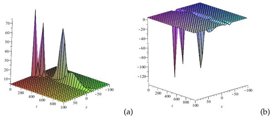
Figure 1.
Profile of 3D wave of the solution (33): (a) u(x,t) and (b) v(x,t) for . The figure illustrates the propagation of single-soliton-like variants with different amplitudes and wavelengths. The variations in their amplitude and wavelength may result from differences in wave energy and speed, influenced by the characteristics of the medium.
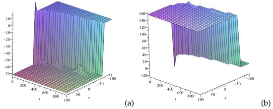
Figure 2.
Profile of 3D wave of the solution (38): (a) u(x,t) and (b) v(x,t) for . The figure illustrates kink-like (a) and anti-kink-like (b) structures, accompanied by atypical periodic-like structures with respect to wave amplitude. The kink-like and anti-kink-like structures represent transitions in the wave field, while the atypical periodic-like structures demonstrate irregular wave oscillations in the studied medium.
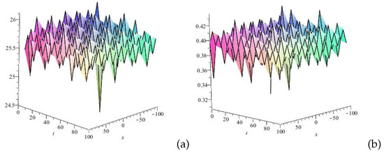
Figure 3.
Profile of 3D wave of the solution (41): (a) u(x,t) and (b) v(x,t) for . The figure illustrates complex soliton-like structures with an almost oscillatory character, where distinct soliton-like waves exhibit different amplitudes and wavelengths. The complex soliton-like structures reflect the influence of various factors on wave propagation. The varying amplitudes and wavelengths indicate unconventional dynamical behavior, where waves exhibit energy changes in a non-conservative manner.
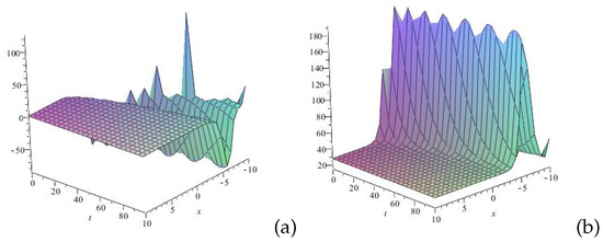
Figure 4.
Profile of 3D wave of the solution (46): (a) u(x,t) and (b) v(x,t) for . The figure illustrates the coexistence of complex soliton-like packets and single-soliton-like waves with different amplitudes and wavelengths. The emergence of soliton-like wave structures with varying amplitudes and wavelengths highlights the role of various factors in shaping wave dynamics, beyond conventional interactions.
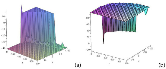
Figure 5.
Profile of 3D wave of the solution (50): (a) u(x,t) and (b) v(x,t) for . The figure depicts complex kink-like (a) and anti-kink-like (b) wave structures accompanied by atypical periodic-like waves with respect to wave amplitudes. The complex kink-like and anti-kink-like structures describe transitions in the wave field. The accompanying atypical periodic-like waves with different amplitudes show irregular decaying and amplifying oscillations in the studied medium.
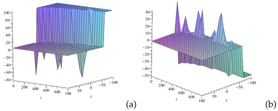
Figure 6.
Profile of 3D wave of the solution (55): (a) u(x,t) and (b) v(x,t) for . The figure depicts the coexistence of complex kink-like (a) and anti-kink-like (b) wave structures, interacting with multiple single-soliton-like waves of different amplitudes and wavelengths. The complex kink-like and anti-kink-like wave structures represent transitions in the wave field, with their evolution influenced by various factors. The coexistence of multiple single-soliton-like waves with varying amplitudes and wavelengths suggests unconventional energy distribution and atypical wave evolution.
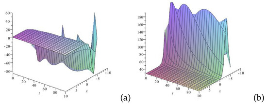
Figure 7.
Profile of 3D wave of the solution (59): (a) u(x,t) and (b) v(x,t) for . The figure illustrates the coexistence of complex soliton-like structures and single-soliton-like waves with different amplitudes and wavelengths. This configuration suggests an unconventional energy distribution and modified wave stability.
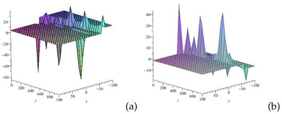
Figure 8.
Profile of 3D wave of the solution (75): (a) u(x,t) and (b) v(x,t) for . The figure depicts the coexistence of complex kink-like (a) and anti-kink-like (b) wave structures, interacting with multiple single-soliton-like waves of different amplitudes, wavelengths, and orientations. The complex kink-like and anti-kink-like structures represent smooth transitions in the wave field. The single-soliton-like waves exhibit a variety of orientations, indicating their ability to self-organize in different spatial and temporal patterns. These structures undergo changes in wave geometry and wave energy distribution as they interact over time.
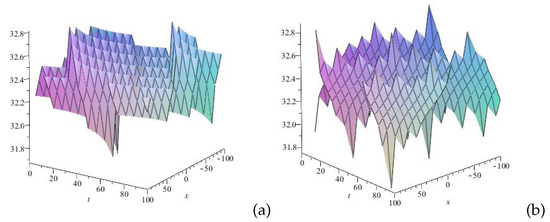
Figure 9.
Profile of 3D wave of the solution (83): (a) u(x,t) and (b) v(x,t) at . The figure illustrates the interweaving of kink-like, anti-kink-like, and soliton-like wave structures. The combination of these three wave types forms a complex structure that facilitates smooth transitions between different wave types, with each influencing the dynamics of the system.
6. Conclusions
In this study, we proposed an extended version of the SEsM, which is applicable for obtaining analytical solutions of FNPDEs, that models dynamics of real-world processes with complex wave behavior. The solutions to such FNPDEs are expressed as combinations of single-composite functions, which involve solutions to two distinct simple equations or two distinct special functions with different independent variables. This is a novel approach in solution’s constructing that is introduced for the first time in finding exact solutions to FNPDEs. A generalized algorithm of the extended SEsM has been also presented, allowing the researcher to flexibly choose an appropriate traveling wave transformation and appropriate simple equations’ types to extract exact solutions to the studied systems of FNPDEs. This highlights the universality of the methodology in its application to various systems of FNPDEs.
One variant of the extended SEsM has been applied to the time-fractional Boussinesq-like system, introducing a fractional traveling wave transformation and utilizing two second-order ODEs with different coordinates in their generalized form as simple equations. It has been demonstrated that, for different numerical values of the coefficients in the polynomial parts of these equations, they reduce to various forms, each yielding distinct analytical solutions. Using different combinations of these solutions, we derived a part of the possible analytical solutions to the studied system of FNPDEs, including diverse combinations of hyperbolic, elliptic, and trigonometric functions. The numerical simulations of some of the analytical solutions confirm that the investigated fractional system exhibits a variety of mixed waves, such as single-soliton-like waves, multi-soliton-like structures with different amplitudes and wavelengths, complex kink and anti-kink-like structures, and periodic-like wave packets. The propagation of such traveling-wave-like structures is considered in terms of the non-conventional (fractional) nature of Equation (1).
The analytical solutions obtained in this study have potential applications in predicting and controlling various physical processes that involve complex wave dynamics. Such physical processes include diffusion in porous media, nanofluid dynamics, ocean current modeling, multiphase fluid dynamics, as well as geophysical phenomena such as sediment transport, deposition in rivers, ocean currents with suspended sediments, and fluid flow through porous media with sedimentation. These phenomena can be effectively described by Equation (1). Therefore, the results presented in this article provide valuable but still incomplete information about the wave behavior of such fractional models. In this sense, they are only the initial strokes in a broader study of the specific wave dynamics of the system (1). Our future research plans include conducting a more in-depth analysis of the results presented here, both analytically and numerically. Through this, we aim to shed more light in the understanding and interpretation of the unconventional multi-wave dynamics of real processes modeled by NPDEs like Equation (1).
Author Contributions
Conceptualization, E.V.N. and M.C.-L.; methodology, E.V.N.; software, E.V.N.; validation, E.V.N. and M.C.-L.; formal analysis, E.V.N. and M.C.-L.; investigation, E.V.N.; data curation, M.C.-L.; writing—original draft preparation, E.V.N.; writing—review and editing, M.C.-L.; visualization, E.V.N. and M.C.-L.; supervision, E.V.N. and M.C.-L.; project administration, E.V.N.; funding acquisition, E.V.N. All authors have read and agreed to the published version of the manuscript.
Funding
E. V. Nikolova would like to thank the Bulgarian National Science Fund for their financial support in funding the project “Artificial intelligence for investigation and modeling of real processes”, KP-06-H82/4.
Data Availability Statement
The original contributions presented in this study are included in the article.
Conflicts of Interest
The author declares no conflict of interest.
References
- Rivero, M.; Trujillo, J.J.; Vázquez, L.; Velasco, M.P. Fractional dynamics of populations. Appl. Math. Comput. 2011, 218, 1089–1095. [Google Scholar] [CrossRef]
- Owolabi, K.M. High-dimensional spatial patterns in fractional reaction-diffusion system arising in biology. Chaos Solitons Fractals 2020, 134, 109723. [Google Scholar] [CrossRef]
- Ghanbari, B.; Günerhan, H.; Srivastava, H.M. An application of the Atangana-Baleanu fractional derivative in mathematical biology: A three-species predator-prey model. Chaos Solitons Fractals 2020, 138, 109910. [Google Scholar] [CrossRef]
- Kulish, V.V.; Lage, J.L. Application of fractional calculus to fluid mechanics. J. Fluids Eng. 2002, 124, 803–806. [Google Scholar] [CrossRef]
- Yıldırım, A. Analytical approach to fractional partial differential equations in fluid mechanics by means of the homotopy perturbation method. Int. J. Numer. Methods Heat Fluid Flow 2010, 20, 186–200. [Google Scholar] [CrossRef]
- Hosseini, V.R.; Rezazadeh, A.; Zheng, H.; Zou, W. A nonlocal modeling for solving time fractional diffusion equation arising in fluid mechanics. Fractals 2022, 30, 2240155. [Google Scholar] [CrossRef]
- Ozkan, E.M. New Exact Solutions of Some Important Nonlinear Fractional Partial Differential Equations with Beta Derivative. Fractal Fract. 2022, 6, 173. [Google Scholar] [CrossRef]
- Fallahgoul, H.; Focardi, S.; Fabozzi, F. Fractional Calculus and Fractional Processes with Applications to Financial Economics: Theory and Application; Academic Press: Cambridge, MA, USA, 2016. [Google Scholar]
- Ara, A.; Khan, N.A.; Razzaq, O.A.; Hameed, T.; Raja, M.A.Z. Wavelets optimization method for evaluation of fractional partial differential equations: An application to financial modelling. Adv. Differ. Equ. 2018, 2018, 8. [Google Scholar] [CrossRef]
- Tarasov, V.E. On history of mathematical economics: Applicatioactionaln of fr calculus. Mathematics 2019, 7, 509. [Google Scholar] [CrossRef]
- Kumar, S. A new fractional modeling arising in engineering sciences and its analytical approximate solution. Alex. Eng. J. 2013, 52, 813–819. [Google Scholar] [CrossRef]
- Sun, H.; Zhang, Y.; Baleanu, D.; Chen, W.; Chen, Y. A new collection of real world applications of fractional calculus in science and engineering. Commun. Nonlinear Sci. Numer. Simul. 2018, 64, 213–231. [Google Scholar] [CrossRef]
- Chen, W.; Sun, H.; Li, X. Fractional Derivative Modeling in Mechanics and Engineering; Springer Nature: Berlin/Heidelberg, Germany, 2022. [Google Scholar]
- Anco, S.C.; Liu, S. Exact solutions of semilinear radial wave equations in n dimensions. J. Math. Phys. 2003, 44, 4103–4117. [Google Scholar] [CrossRef][Green Version]
- Hirota, R. Exact Solution of the Korteweg-de Vries Equation for Multiple Collisions of Solitons. Phys. Rev. Lett. 1971, 27, 1192–1194. [Google Scholar] [CrossRef]
- Wang, M.; Zhou, Y. The Homogeneous Balance Method and Its Application to Nonlinear Equations. Chaos Solitons Fractals 1996, 7, 2047–2054. [Google Scholar] [CrossRef]
- Liu, S.K.; Fu, Z.T.; Liu, S.D.; Zhao, Q. Jacobi Elliptic Function Expansion Method and Periodic Wave Solutions of Nonlinear Wave Equations. Phys. Lett. 2001, 289, 69–74. [Google Scholar] [CrossRef]
- Kudryashov, N.A. Exact soliton solutions of the generalized evolution equations of wave dynamics. J. Appl. Math. Mech. 1988, 55, 372–375. [Google Scholar]
- Wang, M.; Li, X.; Zhang, J. The (G′/G)-expansion method and travelling wave solutions of nonlinear evolution equations in mathematical physics. Phys. Lett. A 2008, 372, 417–423. [Google Scholar] [CrossRef]
- Zhang, J.; Li, Z. The F–expansion method and new periodic solutions of nonlinear evolution equations. Chaos Solitons Fractals 2008, 37, 1089–1096. [Google Scholar] [CrossRef]
- Wazwaz, A.M. The tanh method for traveling wave solutions of nonlinear equations. Appl. Math. Comput. 2004, 154, 713–723. [Google Scholar] [CrossRef]
- Feng, Z. The First Integral Method to Study the Burgers–KdV Equation. J. Phys. Math. Gen. 2002, 35, 343–349. [Google Scholar] [CrossRef]
- He, J.H.; Wu, X.H. Exp-Function Method for Nonlinear Wave Equations. Chaos, Solitons Fractals 2006, 30, 700–708. [Google Scholar] [CrossRef]
- Kudryashov, N.A. Simplest Equation Method to Look for Exact Solutions of Nonlinear Differential Equations. Chaos Solitons Fractals 2005, 24, 1217–1231. [Google Scholar] [CrossRef]
- Vitanov, N.K. On modified method of simplest equation for obtaining exact and approximate solutions of nonlinear PDEs: The role of the simplest equation. Commun. Nonlinear Sci. Numer. Simul. 2011, 16, 4215–4231. [Google Scholar] [CrossRef]
- Vitanov, N.K. Application of Simplest Equations of Bernoulli and Riccati Kind for Obtaining Exact Traveling-Wave Solutions for a Class of PDEs with Polynomial non-linearity. Commun. Non-Linear Sci. Numer. Simul. 2010, 15, 2050–2060. [Google Scholar] [CrossRef]
- Vitanov, N.K. Modified Method of Simplest Equation: Powerful Tool for Obtaining Exact and Approximate Traveling-Wave Solutions of non-linear PDEs. Commun. Non-Linear Sci. Numer. Simul. 2011, 16, 1176–1185. [Google Scholar] [CrossRef]
- Vitanov, N.K. Recent Developments of the Methodology of the Modified Method of Simplest Equation with Application. Pliska Stud. Math. Bulg. 2019, 30, 29–42. [Google Scholar]
- Vitanov, N.K. Modified Method of Simplest Equation for Obtaining Exact Solutions of non-linear Partial Differential Equations: History, recent development and studied classes of equations. J. Theor. Appl. Mech. 2019, 49, 107–122. [Google Scholar] [CrossRef]
- Vitanov, N.K.; Dimitrova, Z.I.; Vitanov, K.N. Simple Equations Method (SEsM): Algorithm, Connection with Hirota Method, Inverse Scattering Transform Method, and Several Other Methods. Entropy 2021, 23, 10. [Google Scholar] [CrossRef]
- Vitanov, N.K. The Simple Equations Method (SEsM) For Obtaining Exact Solutions Of non-linear PDEs: Opportunities Connected to the Exponential Functions. AIP Conf. Proc. 2019, 2159, 030038. [Google Scholar] [CrossRef]
- Dimitrova, Z.I.; Vitanov, K.N. Homogeneous Balance Method and Auxiliary Equation Method as Particular Cases of Simple Equations Method (SEsM). AIP Conf. Proc. 2021, 2321, 030004. [Google Scholar] [CrossRef]
- Dimitrova, Z.I. On several specific cases of the simple equations method (SEsM): Jacobi elliptic function expansion method, F-expansion method, modified simple equation method, trial function method, general projective Riccati equations method, and first intergal method. AIP Conf. Proc. 2022, 2459, 030006. [Google Scholar] [CrossRef]
- Vitanov, N.K. Simple equations method (SEsM) and nonlinear PDEs with fractional derivatives. AIP Conf. Proc. 2022, 2459, 030040. [Google Scholar] [CrossRef]
- Zhang, S.; Zhang, H.-Q. Fractional sub-equation method and its applications to nonlinear fractional PDEs. Phys. Lett. A 2011, 375, 1069–1073. [Google Scholar] [CrossRef]
- Guo, S.; Mei, L.; Li, Y.; Sun, Y. The improved fractional sub-equation method and its applications to the space-time fractional differential equations in fluid mechanics. Phys. Lett. A 2012, 376, 407–411. [Google Scholar] [CrossRef]
- Lu, B. Backlund transformation of fractional Riccati equation and its applications to nonlinear fractional partial differential equations. Phys. Lett. A 2012, 376, 2045–2048. [Google Scholar] [CrossRef]
- Zheng, B.; Wen, C. Exact solutions for fractional partial differential equations by a new fractional sub-equation method. Adv. Differ. Equ. 2013, 2013, 199. [Google Scholar] [CrossRef]
- Zheng, B. A new fractional Jacobi elliptic equation method for solving fractional partial differential equations. Adv. Differ. Equ. 2014, 2014, 228. [Google Scholar] [CrossRef]
- Feng, Q.; Meng, F. Explicit solutions for space-time fractional partial differential equations in mathematical physics by a new generalized fractional Jacobi elliptic equation-based sub-equation method. Optik 2016, 127, 7450–7458. [Google Scholar] [CrossRef]
- Vitanov, N.K. Simple Equations Method (SEsM): An Effective Algorithm for Obtaining Exact Solutions of Nonlinear Differential Equations. Entropy 2022, 24, 1653. [Google Scholar] [CrossRef]
- Vitanov, N.K. Simple equations method (SEsM): Review and new results. Aip Conf. Proc. 2022, 2459, 020003. [Google Scholar] [CrossRef]
- Vitanov, N.K.; Bugay, A.; Ustinov, N. On a Class of Nonlinear Waves in Microtubules. Mathematics 2024, 12, 3578. [Google Scholar] [CrossRef]
- Vitanov, N.K. On the Method of Transformations: Obtaining Solutions of Nonlinear Differential Equations by Means of the Solutions of Simpler Linear or Nonlinear Differential Equations. Axioms 2023, 12, 1106. [Google Scholar] [CrossRef]
- Nikolova, E.V. Exact Travelling-Wave Solutions of the Extended Fifth-Order Korteweg-de Vries Equation via Simple Equations Method (SEsM): The Case of Two Simple Equations. Entropy 2022, 24, 1288. [Google Scholar] [CrossRef] [PubMed]
- Zhou, J.; Ju, L.; Zhao, S.; Zhang, Y. Exact Solutions of Nonlinear Partial Differential Equations Using the Extended Kudryashov Method and Some Properties. Symmetry 2023, 15, 2122. [Google Scholar] [CrossRef]
- Nikolova, E.V. Numerous Exact Solutions of the Wu-Zhang System with Conformable Time–Fractional Derivatives via Simple Equations Method (SEsM): The Case of Two Simple Equations. Springer Proc. Math. Stat. 2024, 449, 231–241. [Google Scholar] [CrossRef]
- Nikolov, R.G.; Nikolova, E.V.; Boutchaktchiev, V.N. Several Exact Solutions of the Fractional Predator—Prey Model via the Simple Equations Method (SEsM). Springer Proc. Math. Stat. 2024, 449, 277–287. [Google Scholar] [CrossRef]
- Nikolova, E.V. On the Traveling Wave Solutions of the Fractional Diffusive Predator—Prey System Incorporating an Allee Effect. Springer Proc. Math. Stat. 2024, 449, 267–276. [Google Scholar] [CrossRef]
- Nikolova, E.V. On the Extended Simple Equations Method (SEsM) and Its Application for Finding Exact Solutions of the Time-Fractional Diffusive Predator–Prey System Incorporating an Allee Effect. Mathematics 2025, 13, 330. [Google Scholar] [CrossRef]
- Sachs, R.L. On the integrable variant of the boussinesq system: Painlevé property, rational solutions, a related many-body system, and equivalence with the AKNS hierarchy. Phys. Nonlinear Phenom. 1988, 30, 1–27. [Google Scholar] [CrossRef]
- Jumarie, G. Modified Riemann-Liouville derivative and fractional Taylor series of non-differentiable functions further results. Focuses on analytical methods using fractional transforms. Comput. Math. Appl. 2006, 51, 1367–1376. [Google Scholar] [CrossRef]
- Jumarie, G. Laplace’s transform of fractional order via the Mittag-Leffler function and modified Riemann-Liouville derivative. Appl. Math. Lett. 2009, 22, 1659–1664. [Google Scholar] [CrossRef]
- Jumarie, G. Table of some basic fractional calculus formulae derived from a modified Riemann-Liouville derivative for non-differentiable functions. Appl. Math. Lett. 2009, 22, 378–385. [Google Scholar] [CrossRef]
- Khalil, R.; Al Horani, M.; Yousef, A.; Sababheh, M. A new definition of fractional derivative. J. Comput. Appl. Math. 2014, 264, 65–70. [Google Scholar] [CrossRef]
- Li, Z.-B.; He, J.-H. Fractional Complex Transform for Fractional Differential Equations. Math. Comput. Appl. 2010, 15, 970–973. [Google Scholar] [CrossRef]
- Vitanov, N.K.; Dimitrova, Z.I.; Ivanova, T.I. On solitary wave solutions of a class of nonlinear partial differential equations based on the function 1/coshn(αx+βt). Appl. Math. Comput. 2017, 315, 372–380. [Google Scholar] [CrossRef]
- Nikolova, E.V.; Chilikova-Lubomirova, M.; Vitanov, N.K. Exact solutions of a fifth—order Korteweg–de Vries –type equation modeling nonlinear long waves in several natural phenomena. AIP Conf. Proc. 2021, 2321, 030026. [Google Scholar] [CrossRef]
- Hendi, A. New exact travelling wave solutions for some nonlinear evolution equations. Int. J. Nonlinear Sci. 2009, 7, 259–267. [Google Scholar]
- Zhang, H. New exact travelling wave solutions for some nonlinear evolution equations. Chaos Solitons Fractals 2005, 26, 921–925. [Google Scholar] [CrossRef]
- Saied, E.A.; Abd El-Rahman, R.G.; Ghonamy, M.I. A generalized Weierstrass elliptic function expansion method for solving some nonlinear partial differential equations. Comput. Math. Appl. 2009, 58, 1725–1735. [Google Scholar] [CrossRef][Green Version]


Disclaimer/Publisher’s Note: The statements, opinions and data contained in all publications are solely those of the individual author(s) and contributor(s) and not of MDPI and/or the editor(s). MDPI and/or the editor(s) disclaim responsibility for any injury to people or property resulting from any ideas, methods, instructions or products referred to in the content. |
© 2025 by the authors. Licensee MDPI, Basel, Switzerland. This article is an open access article distributed under the terms and conditions of the Creative Commons Attribution (CC BY) license (https://creativecommons.org/licenses/by/4.0/).