A Two-Step Sequential Hyper-Reduction Method for Efficient Concurrent Nonlinear FE² Analyses

Abstract

In this paper, we propose a two-step sequential hyper-reduction method to significantly enhance computational efficiency for both macro- and micro-level analyses in concurrent nonlinear FE² multiscale simulations. In general, one of the major computational burdens of nonlinear FE² problems is the repetitive micro-level analysis, which must be performed at all integration points of the macroscopic structure. We propose adopting the discrete empirical interpolation method (DEIM) for both macroscopic and microscopic problems, achieving a significant reduction in the number of integration points in both models. The proposed two-step sequential framework aligns with reduced-order modeling, enabling an efficient multiscale procedure for concurrent nonlinear FE² analysis in the online stage. We verified the accuracy and efficiency of FE² analysis using the proposed method through a simple example.

1. Introduction

In various industries such as defense, aerospace, automotive, etc., ongoing research efforts are focused on the development of advanced composite materials aiming at reducing structural weight and enhancing mechanical performance. In particular, advanced composite materials usually have complex microstructures that are a mixture of various materials. Thus, achieving accurate prediction of the mechanical behaviors of structures composed of such materials is not a simple task, particularly if we consider the nonlinearities of the given composite materials and structures. Multiscale analysis is a method to predict such complex behavior of structures by comprehensively considering physical phenomena occurring at different scales. It can produce accurate analysis results, especially in cases where the microstructure significantly impacts macroscopic behavior. Among them, the FE² method performs simultaneous and mutual computational processes by linking macroscopic and microscopic finite element models. The macroscopic model analyzes the behavior of the entire structure, and the microscopic model computes local material properties and deformation characteristics. This approach allows the expression of the complex nonlinear behaviors of the composite material to be reproduced more realistically. However, FE² analysis has the disadvantage of high computational cost because the microstructure analysis should be performed repetitively at all integration points of the macrostructure. Also, the computational resources and time increase exponentially as the problem size increases, which causes huge computational inefficiency. Thus, various approaches, such as the second homogenization technique [1,2,3], parallel computing method [4], data-driven [5] or data-driven-based modeling using machine learning [6,7,8], and a direct FE² technique [9,10,11,12] have been proposed to improve the efficiency of FE² analysis.

In particular, the approach utilizing a reduced-order model (ROM) is an effective method for increasing computational efficiency by reducing the size of unknown variables and thus contributing to a reduction in computational complexity. Various model order reduction methods have been proposed so far, e.g., proper generalized decomposition (PGD), as well as proper orthogonal decomposition (POD) methods. PGD [13,14] is based on the separation of variables, in which the solution is represented as a sum of separable one-dimensional functions according to each of the problem dimensions or parameters. As a result, PGD has a very low online computational cost due to simple summation operations, but it has a convergence sensitivity to nonlinearity and high implementation complexity as well. POD is a method that reflects the behavioral characteristics of the model through the basis. POD guarantees high accuracy, and it is simple to implement because it only requires performing singular value decomposition (SVD) of the snapshot matrix. Therefore, POD-based methods have been utilized in various fields [15,16,17,18,19,20,21]. However, this method is inefficient for nonlinear problems because all finite elements should be evaluated in the online stage. Therefore, hyper-reduction techniques have been proposed to improve the efficiency of nonlinear systems, which can be categorized into ones that use the cubature method or the empirical interpolation method (EIM) [22].

First, the cubature method [23] reduces the cost of nonlinear integration calculations using reduced and weighted integration points (or elements), minimizing integration errors. In other words, it reduces the integration cost by minimizing the evaluation times of nonlinear terms. Since Hernández et al. [24] first applied the cubature method to FE² analysis, many researchers have proposed modified versions suitable for FE² analysis [25,26,27,28,29]. Second, EIM is an approach to reduce computational costs by interpolating nonlinear terms. Most EIMs use the basis of the system obtained by POD as a projector and approximate the response of the actual model based on Galerkin projection. Since EIM is mode-based, stress reconstruction is easier and more accurate than with the cubature method. Due to these characteristics, EIM-based approaches have been widely used to solve various scientific and engineering problems [30,31,32,33,34]. A representative example is the discrete empirical interpolation method (DEIM) [35], which is an improved version suitable for discretized models. In the case of FE² analysis, Soldner et al. [36,37] focused on robustness and applied interpolation-based model order reduction methods to the FE² method with comprehensive reviews. The methods introduced above were applied to a microscopic domain for improvement in the online efficiency of nonlinear FE² analysis.

In the present work, we propose a two-step sequential hyper-reduction method to substantially enhance the efficiency of FE² analysis by constructing a macroscopic ROM based on the DEIM that has not been simultaneously adapted to FE² analysis with an ROM in a microscopic problem. Since one of the major bottlenecks for efficiency improvement of FE² analysis is the high-fidelity modeling of a microscopic structure and its solution process, most research has focused on directly reducing the computation time in the microscopic domain. However, these previous approaches still require repeatedly evaluating the microscopic model at every integration point in the macroscopic domain, which may be inefficient for complex or high-dimensional macroscale models. To overcome these limitations, this study mainly focused on reducing the number of executions of the microscopic problem and improving online efficiency greatly by constructing an ROM of the macroscopic model. In this paper, we investigated the performance of the proposed method by dividing it into three different types of ROM construction: at a microscopic level, a macroscopic level, and a combination of both. Whereas the previous method hardly achieved the “online” capability due to the computations in the macroscopic domain, the proposed method showed a significant improvement in online efficiency.

The paper is organized as follows: Section 2 briefly introduces FE² analysis and the model order reduction technique proposed in this study. Section 3 presents numerical examples to validate the accuracy and efficiency of the proposed method. Section 4 provides conclusions, including suggestions for future research topics.

2. Mathematical Formulation

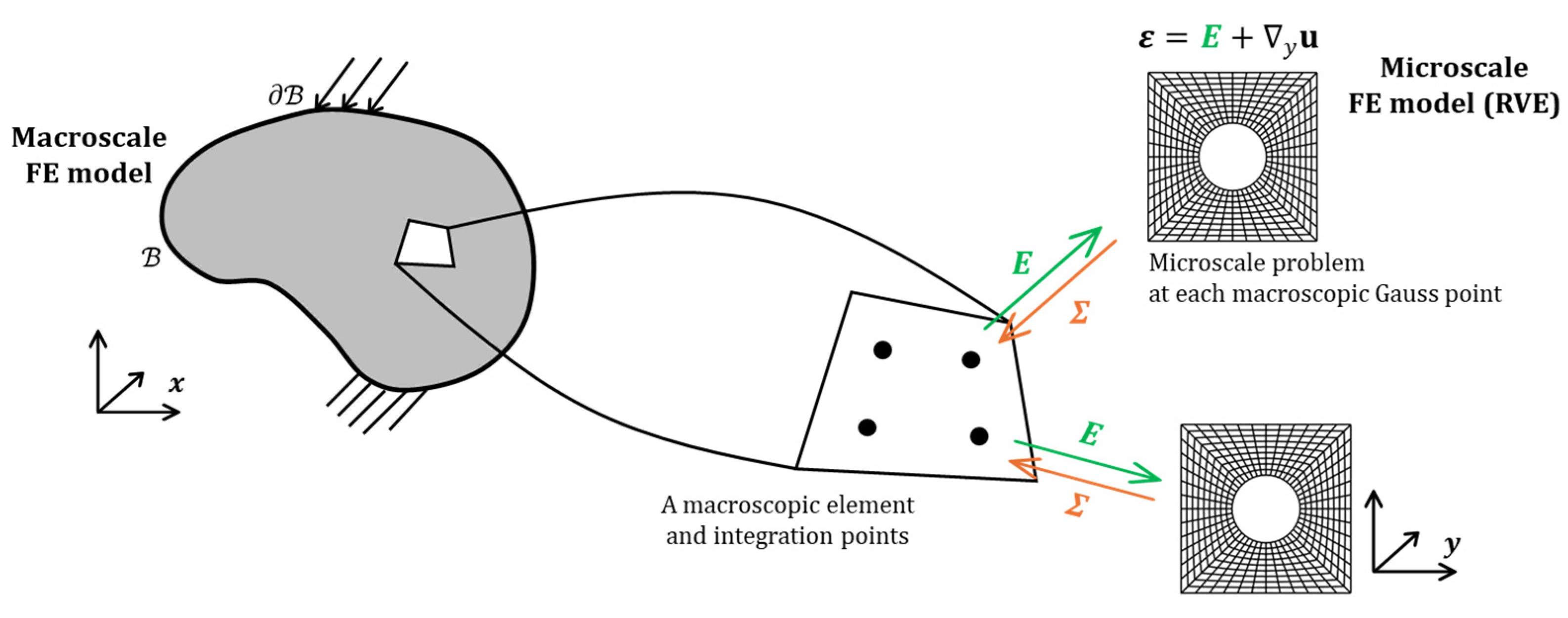
2.1. Brief Review of Nonlinear Multiscale Finite Element Method (FE² Method)

When we assume the microstructure has a sufficiently smaller scale than the macrostructure, we can possibly predict the behavior of the macrostructure through the homogenization of responses for the microstructure. The transition relationship between microscopic and macroscopic scales is based on the Hill–Mandel condition [38,39,40], which states that the volume-averaged variation of work on the microscale equals the variation of local work on the macroscale, according to the energy consistency principle. The Hill–Mandel condition is as follows:

$${\displaystyle \frac{1}{\left|Y\right|}}{\int }_Y\mathit{\sigma }:\delta \mathit{\epsilon }dV=\mathit{\Sigma }:\delta \mathit{E}$$

(1)

where $\mathit{\Sigma }$ and $\mathit{\sigma }$ represent the macroscopic and microscopic stress tensor, respectively. $\delta \mathit{E}$ and $\delta \mathit{\epsilon }$ denote the variation of the macroscopic and microscopic strains, respectively. $\left|Y\right|$ is the volume of a microscopic domain $Y$. The behavior of the macrostructure depends on the boundary deformation applied to the microscopic domain. Among the boundary conditions of various RVE models for satisfying the Hill–Mandel condition, we applied the periodic boundary condition (PBC) in this study. The PBC for the RVE model is applied, as expressed in Equation (2):

$${\mathbf{u}}^{+}-{\mathbf{u}}^{-}=\mathit{E}·\left({\mathbf{y}}^{+}-{\mathit{y}}^{-}\right) \mathrm{on} \partial V,$$

(2)

where $\mathbf{y}$ is the nodal coordinate of the microscopic FE model. The signs ‘+’ and ‘−’ are used to denote the boundary nodes corresponding to the top–bottom, and right–left sides of the RVE. $\mathbf{u}$ is the microscopic displacement. Therefore, the macroscale stress tensor can be expressed (Equation (3)) as the volume average of the microscale stress tensor based on the Hill–Mandel energy consistency relation applying PBC. The detailed derivation is shown in [35,36,37,38,39,40,41]:

$$\mathit{\Sigma }\left(\mathbf{x}\right)={\displaystyle \frac{1}{\left|Y\right|}}{\int }_Y\mathit{\sigma }\left(\mathbf{x},\mathbf{y}\right)dV$$

(3)

As illustrated in Figure 1, the FE² method divides a given model into two scales, a macroscopic domain $\mathcal{B}$ and the microscopic domain $Y$, and simultaneously analyzes in two different scales. To this end, the boundary value problems (BVPs) of both scales should be satisfied, as expressed in Equations (4) and (5):

$${\int }_{\mathcal{B}}{\nabla }_x\overline{\mathbf{U}}:\mathit{\Sigma }dx={\int }_{\mathcal{B}}{\rho }^H\mathit{b}·\overline{\mathbf{U}}dx+{\int }_{\partial \mathcal{B}}\mathit{T}·\overline{\mathbf{U}}ds, \forall \overline{\mathbf{U}}\in \mathcal{B}.$$

(4)

$${\int }_Y{\nabla }_y\overline{\mathbf{u}}:\mathit{\sigma }dy=0, \forall \overline{\mathbf{u}}\in Y,$$

(5)

where $\overline{\mathbf{U}}$ and $\overline{\mathbf{u}}$ are the virtual displacement fields in the macroscopic and microscopic domains, respectively. $\mathit{T}$ is a traction force vector acting on the boundary $\partial \mathcal{B}$, $\mathit{b}$ is a body force acting on the region $\mathcal{B}$, and ${\rho }^H$ is the average density of an entire macroscale structure. ${\nabla }_x$ and ${\nabla }_y$ denote differentiation operators that represent the gradient with respect to $x$ and $y$, respectively. The microscopic stress and strain are computed as follows:

$$\mathit{\sigma }\left(\mathbf{x},\mathbf{y}\right)={\displaystyle \frac{\partial W\left(\mathbf{y},\mathit{\epsilon }\right)}{\partial \mathit{\epsilon }}}, \mathit{\epsilon }\left(\mathbf{x},\mathbf{y}\right)=sym\left({\nabla }_x\mathbf{U}\left(\mathbf{x}\right)+{\nabla }_y\mathbf{u}\left(\mathbf{x},\mathbf{y}\right)\right),$$

(6)

where $\mathbf{U}\left(\mathbf{x}\right)$ is macroscopic displacement. $W\left(\mathbf{y},\mathit{\epsilon }\right)$ is the strain energy density function. $sym\left(·\right)$ represents a symmetric part of a second-order tensor. The behavior of the macrostructure depends on the boundary deformation applied to the microscopic domain.

When we perform FE² analysis for a nonlinear macroscopic model, the tangent moduli of the macroscale domain change at each iteration. The tangent moduli are defined as follows:

$${\mathbb{C}}^{\left(j,i\right)}≔{\displaystyle \frac{\partial {\mathit{\Sigma }}^{\left(j,i\right)}}{\partial {\mathit{E}}^{\left(j,i\right)}}},$$

(7)

where $i$ is the iteration, and $j$ represents a load step in a macroscale. Here, the evaluation process of the macroscopic tangent moduli is called tangential homogenization. The detailed formulation is described in [4,42]:

2.2. Proper Orthogonal Decomposition-Based Discrete Empirical Interpolation Method (POD-DEIM)

The discrete empirical interpolation method (DEIM) introduced by Chaturantabut and Sorensen [35] is a discretized form of the EIM [43], which is a hyper-reduction for nonlinear systems that perform integration only with specific sample elements. In other words, the DEIM approximates the full-order model (FOM) based on the information obtained at only a portion of all elements. Radermacher and Reese [44] developed a DEIM based on POD for nonlinear solid mechanics system. The nonlinear system is expressed as follows:

$$\mathbf{F}\left(\mathbf{U}\right):=\mathbf{R}\left(\mathbf{U}\right)-\mathbf{P}=\mathbf{0},$$

(8)

where $\mathbf{U}\in {\mathbb{R}}^{N\times 1}$ is a vector of nodal displacements. $\mathbf{R}\left(\mathbf{U}\right)\in {\mathbb{R}}^{N\times 1}$ and $\mathbf{P}\in {\mathbb{R}}^{N\times 1}$ are the vectors of internal forces and the external forces, respectively. $N$ denotes the degrees of freedom (DOFs) of the system. The displacement and internal force vectors are approximated as follows:

$$\mathbf{U}\approx \tilde{\mathbf{U}}=\mathsf{\Phi }{\mathbf{U}}_r,$$

(9)

$$\mathbf{R}\left(\mathbf{U}\right)\approx \tilde{\mathbf{R}}\left(\mathbf{U}\right)=\mathsf{\Omega }{\mathbf{R}}_r\left(\mathbf{U}\right),$$

(10)

where $\mathsf{\Phi }=\left[{\mathit{\varphi }}_1,\dots ,{\mathit{\varphi }}_k\right]\in {\mathbb{R}}^{N\times k}$ and $\mathsf{\Omega }=\left[{\mathit{\omega }}_1,\dots ,{\mathit{\omega }}_k\right]\in {\mathbb{R}}^{N\times k}$ represent the bases of the displacement field and nonlinear term, respectively. We obtained these bases via POD using the snapshot method. To determine the unknown reduced vector ${\mathbf{R}}_r\left(\mathbf{U}\right)$, we selected the appropriate $k$ DEIM interpolation points from Algorithm 1. The $k$ DEIM interpolation points were chosen so that the approximation error of $\mathbf{R}\left(\mathbf{U}\right)$ was minimized. With the POMs that are expressed by a set of column vectors, the selection process of the DEIM points starts by choosing the first interpolation index ${\mathrm{\wp }}_1\in \left\{1,\dots ,k\right\}$ corresponding to the entry of the first input basis vector ${\mathit{\omega }}_1$ with the largest magnitude. The remaining interpolation indices ${\mathrm{\wp }}_n$ $\left(n=2,\dots ,k\right)$ were chosen by maximizing the residual $\mathbf{r}={\mathit{\omega }}_n-\widehat{\mathsf{\Omega }}{\mathbf{R}}_r$. Thus, Algorithm 1 outputs a matrix $\mathbf{Z}$ consisting of $k$ logical vectors that represent the indices of the DEIM points. Multiplying ${\mathbf{Z}}^T$ into Equation (10) gives

$${\mathbf{Z}}^T\mathbf{R}={\mathbf{Z}}^T\mathsf{\Omega }{\mathbf{R}}_r\left(\mathbf{U}\right).$$

(11)

Thus, ${\mathbf{R}}_r\left(\mathbf{U}\right)$ is expressed as follows:

$${\mathbf{R}}_r\left(\mathbf{U}\right)={\left({\mathbf{Z}}^T\mathsf{\Omega }\right)}^{-1}{\mathbf{Z}}^T\mathbf{R}.$$

(12)

${\mathbf{R}}_r\left(\mathbf{U}\right)\in {\mathbb{R}}^{k\times 1}$ contains information corresponding to the DEIM points. Then, we inserted Equations (9), (10) and (12) into Equation (8), applying the Galerkin projection, and we found the reduced nonlinear system:

$$\begin{array}{ll}\tilde{\mathbf{F}}\left({\mathbf{U}}_r\right)& :={\mathsf{\Phi }}^T\tilde{\mathbf{R}}\left(\mathsf{\Phi }{\mathbf{U}}_r\right)-{\mathsf{\Phi }}^T\mathbf{P}\\ & ={\mathsf{\Phi }}^T\mathsf{\Omega }{\left({\mathbf{Z}}^T\mathsf{\Omega }\right)}^{-1}{\mathbf{Z}}^T\tilde{\mathbf{R}}\left(\mathsf{\Phi }{\mathbf{U}}_r\right)-{\mathsf{\Phi }}^T\mathbf{P}\\ & ={\mathbf{M}}_{DEIM}{\mathbf{Z}}^T\tilde{\mathbf{R}}\left(\mathsf{\Phi }{\mathbf{U}}_r\right)-{\mathsf{\Phi }}^T\mathbf{P}\\ & =\mathbf{0}.\end{array}$$

(13)

Using Equation (13), we solved only $k$ evaluations of the nonlinear functions. The Newton–Raphson scheme for nonlinear analysis leads to the following iterative solutions algorithm:

$$\begin{array}{cc}\tilde{\mathbf{F}}\left({\mathbf{U}}_{r,\left(i\right)}^j\right)+\left({\mathbf{M}}_{DEIM}{\mathbf{Z}}^T{\mathbf{K}}_T\left(\mathsf{\Phi }{\mathbf{U}}_{r,\left(i\right)}^j\right)\mathsf{\Phi }\right)∆{\mathbf{U}}_{r,\left(i+1\right)}^j\hfill & =\mathbf{0}\hfill \\ \hfill {\mathbf{U}}_{i+1}^j& ={\mathbf{U}}_i^j+\mathsf{\Phi }∆{\mathbf{U}}_{r,\left(i+1\right)}^j\hfill \\ \hfill ‖\tilde{\mathbf{F}}\left({\mathbf{U}}_{r,\left(i\right)}^j\right)‖& \le tol\hfill \\ \hfill i& \leftarrow i+1\hfill \end{array}$$

(14)

Again, $i$ is the $i$th iteration, and $j$ is the $j$th load step. Further details are presented in [44].

Algorithm 1. Sampling point selection of the DEIM [35]

1: Input: $\mathsf{\Omega }\in {\mathbb{R}}^{N\times k}$ 2: Output: $\mathbf{Z}\in {\mathbb{R}}^{N\times k}$ 3: $\left[\left|\lambda \right|,{\wp }_1\right]=\max \left\{\left|{\mathit{\omega }}_1\right|\right\}$ 4: $\widehat{\mathsf{\Omega }}=\left[{\mathit{\omega }}_1\right],\mathbf{Z}=\left[{\mathit{e}}_{{\wp }_1}\right],\overrightarrow{\wp }=\left[{\wp }_1\right]$ 5: for $n=2$ to $k$ do 6:     Solve $\left({\mathbf{Z}}^T\widehat{\mathsf{\Omega }}\right){\mathbf{R}}_r={\mathbf{Z}}^T{\mathit{\omega }}_n$ for ${\mathbf{R}}_r$ 7:     $\mathbf{r}={\mathit{\omega }}_n-\widehat{\mathsf{\Omega }}{\mathbf{R}}_r$ 8:     $\left[\left|\lambda \right|,{\wp }_n\right]=\max \left\{\left|\mathbf{r}\right|\right\}$ 9:     $\widehat{\mathsf{\Omega }}\leftarrow \left[\begin{array}{cc}\widehat{\mathsf{\Omega }}& {\mathit{\omega }}_n\end{array}\right],\mathbf{Z}\leftarrow \left[\begin{array}{cc}\mathbf{Z}& {\mathit{e}}_{{\wp }_n}\end{array}\right],\overrightarrow{\wp }\leftarrow \left[\begin{array}{c}\wp \\ {\wp }_n\end{array}\right]$ 10: end for

2.3. A Two-Step, Sequential Hyper-Reduction Method for Nonlinear FE² Analysis

As stated in the previous section, sparse integration provides an efficient approximation of the domain of interest to be integrated in both scales. The computational processes of ROM construction were conducted sequentially. In the microscopic problem, the quantities were approximated in the sparse microscopic domain denoted by $Y_s$, such that

$$\mathit{\Sigma }\left(\mathbf{x}\right)\approx \tilde{\mathit{\Sigma }}\left(\mathbf{x}\right)={\displaystyle \frac{1}{\left|Y_s\right|}}\bigcup _{k_i=1}^{n_{e,i}}{\int }_{V_{\left(k_i\right)}}\mathit{\sigma }\left(\mathbf{x},\mathbf{y}\right)dV$$

(15)

$$\mathit{E}\left(\mathbf{x}\right)\approx \tilde{\mathit{E}}\left(\mathbf{x}\right)={\displaystyle \frac{1}{\left|Y_s\right|}}{\bigcup }_{k_i=1}^{n_{e,i}}{\int }_{V_{\left(k_i\right)}}\mathit{\epsilon }\left(\mathbf{x},\mathbf{y}\right)dV={\nabla }_x\overline{\mathbf{U}}\left(\mathbf{x}\right)$$

(16)

$${\mathbb{C}}_{ijkl}\left(\mathbf{x}\right)\approx {\tilde{\mathbb{C}}}_{ijkl}\left(\mathbf{x}\right)={\displaystyle \frac{1}{\left|Y_s\right|}}\bigcup _{k_i=1}^{n_{e,i}}{\int }_{V_{\left(k_i\right)}}\left({\mathbb{c}}_{ijkl}-{\mathbb{c}}_{ijqr}{\displaystyle \frac{\partial {\chi }_q^{kl}}{\partial y_r}}\right)dV$$

(17)

where $\bigcup$ represents the assemblage of elements considering the inter-element connectivity. $k_i$ is an index for the sparse integration, and $n_{e,i}\ll n_e$ denote the number of elements selected by the DEIM algorithm in the microscopic problem. The homogenized stress and tangent moduli obtained in Equations (15) and (17) were used for the macroscopic problem. The overall computational process of the proposed method in microscopic problem is presented in Algorithm 2.

Algorithm 2. Microscopic problem applying the DEIM based on displacement control

1: Input: $\mathit{E}$ 2: Output: ${\tilde{\mathit{\Sigma }}}_H,{\tilde{\mathbb{C}}}_H$ 3: Apply periodic boundary conditions ${\mathbf{u}}^{+}-{\mathbf{u}}^{-}=\mathit{E}·\left({\mathbf{y}}^{+}-{\mathbf{y}}^{-}\right) on \partial V$ 4: for $j_i=1$ to $H$ do 5:    $\mathbf{u}\leftarrow {\mathbf{u}}^{\left(j_i\right)}$ 6:    $i_i\leftarrow 1$ 7:    while not converged do 8:           for $k_i=1$ to $n_{e,i}$ do 9:                  Compute ${\mathit{k}}_T$, ${\mathbf{f}}_{int}$, $\overline{\mathit{\sigma }},\overline{\mathbb{c}}$ 10:         end for 11:         ${\mathit{k}}_{T,r}\leftarrow {\mathbf{m}}_{DEIM}{\mathbf{z}}^T{\mathit{k}}_T\mathsf{\varphi }$ 12:         ${\mathbf{f}}_{int,r}\leftarrow$ ${\mathbf{m}}_{DEIM}{\mathbf{z}}^T{\mathbf{f}}_{int}$ 13:              if $i_i=1$ 14:                  $\mathbf{p}\leftarrow -{\mathit{k}}_T\mathbf{u}$ 15:                  ${\mathbf{p}}_r\leftarrow {\mathbf{m}}_{DEIM}{\mathbf{z}}^T\mathbf{p}$ 16:                  $\mathrm{d}{\mathbf{u}}_r\leftarrow -{\mathit{k}}_{T,r}^{-1}\left({\mathbf{p}}_r+{\mathbf{f}}_{int,r}\right)$ 17:              else 18:                  $\mathrm{d}{\mathbf{u}}_r\leftarrow$ $-{\mathit{k}}_T^{-1}{\mathbf{f}}_{int}$ 19:              end if 20:         $\mathrm{d}\tilde{\mathbf{u}}\leftarrow \mathsf{\varphi }\mathrm{d}{\mathbf{u}}_r$ 21:         $\tilde{\mathbf{u}}\leftarrow \tilde{\mathbf{u}}+\mathrm{d}\tilde{\mathbf{u}}$ 22:         Convergence check 23:         $i_i\leftarrow i_i+1$ 24:    end while 25: end for 26: ${\tilde{\mathit{\Sigma }}}_H\left(\mathbf{x}\right)={\displaystyle \frac{1}{\left|Y_s\right|}}\tilde{\mathit{\sigma }}\left(\mathbf{x},\mathbf{y}\right)$ 27: ${\tilde{\mathbb{C}}}_H={\displaystyle \frac{1}{\left|Y_s\right|}}\tilde{\mathbb{c}}\left(\mathbf{x},\mathbf{y}\right)$

In Algorithm 2, the homogenized quantities are represented by the subscript ‘$H$’, and the reduced variables are denoted by the upper tilde, $\widetilde{•}$.

Following the procedure of the nonlinear FE² analysis, the main process of the proposed macroscopic problem is presented in Algorithm 3. The nested structure contains the solution process of the microscopic problem given in Algorithm 2. Compared with the FOM and previous ROM-based FE² methods, line 6 is one of the major sources of efficiency enhancement due to the decreased number of elements in the macroscopic model. The rest of the algorithms are the same as those of the conventional Newton–Raphson procedure of the FE² analysis.

Algorithm 3. Macroscopic problem applying the DEIM

1: Select sampling point from Algorithm 1 2: for $j_a=1$ to $L$ do 3:     ${\mathbf{P}}_r^{\left(j_a\right)}\leftarrow {\mathbf{M}}_{DEIM}{\mathbf{Z}}^T{\mathbf{P}}^{\left(j_a\right)}$ 4:     $i_a\leftarrow 1$ 5:     while not converged do 6:          for $k_a=1$ to $n_{e,a}$ do 7:              $\mathit{E}\leftarrow {\displaystyle \frac{1}{2}}({\mathit{F}}^T\mathit{F}-\mathbf{1})$ 8:              Obtain ${\tilde{\mathit{\Sigma }}}_H,{\tilde{\mathbb{C}}}_H$ and by solving the microscopic problem (Algorithm 2) 9:              Compute ${\mathit{K}}_T$ and ${\mathbf{F}}_{int}$ 10:          end for 11:          Compute Equation (14) 12:          $i_a\leftarrow i_a+1$ 13:      end while 14: end for

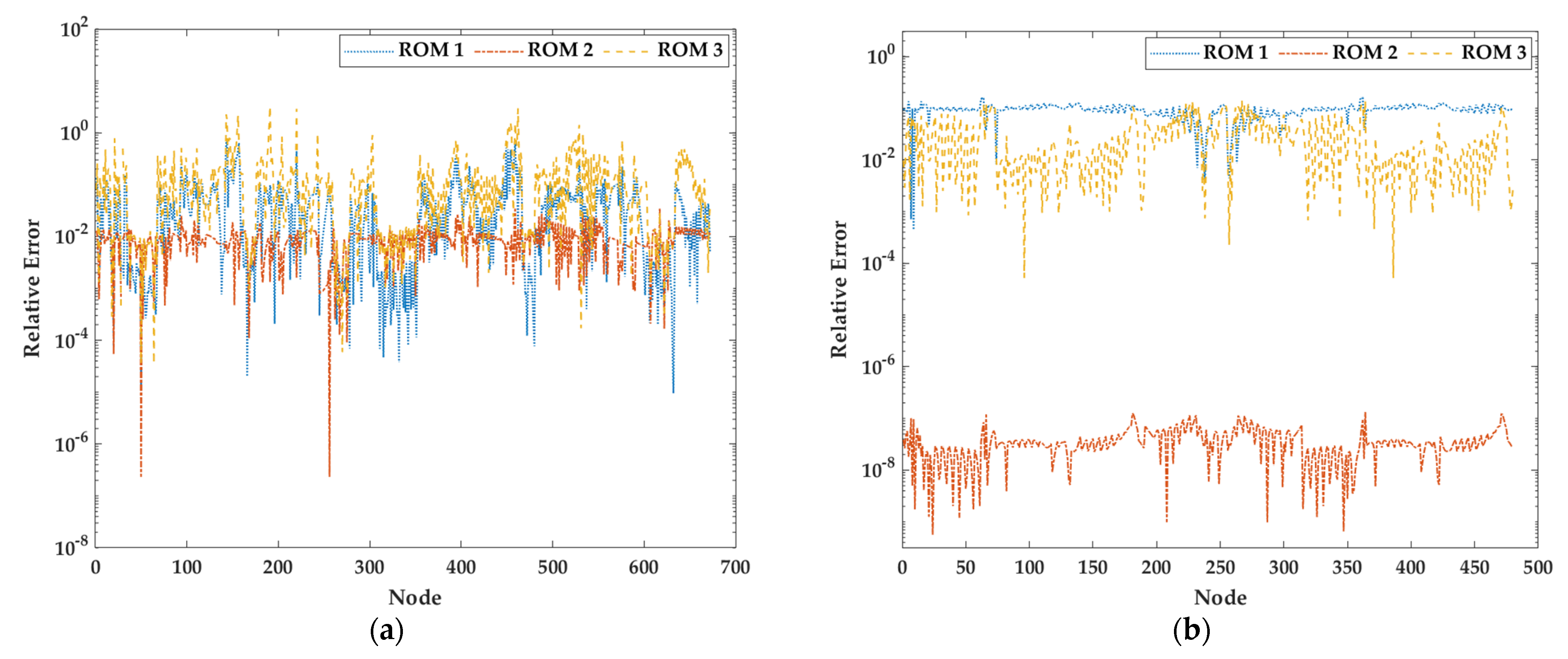
3. Numerical Examples

In this study, we verified the efficiency and accuracy of the proposed FE² analysis using two different structural models. In Section 3.1, a two-dimensional simple beam model with a clamped end is introduced, and in Section 3.2, a microgripper model with complex geometry is selected. All examples present results utilizing the following ROMs:

• ROM 1: ROM of Algorithm 2 applied in the microscopic domain;
• ROM 2: ROM of Algorithm 3 applied in the macroscopic domain;
• ROM 3: combination of ROM 1 and ROM 2 (proposed).

The microscopic model assumed a dimensionless rectangular unit square RVE with one hole in the center. We applied periodic boundary conditions. The RVE model is composed of a hyperelastic material assumed to be the incompressible Mooney–Rivlin model, as shown in Equation (18) [45]:

$$W\left(I_1,I_2\right)=A_{10}\left(I_1-3\right)+A_{01}\left(I_2-3\right),$$

(18)

where $I_i$ represent invariants, and $A_{ij}$ are material constants. For finite element modeling, a four-node plane stress element was used. All computations were conducted by MATLAB R2024a in a Windows 10 environment. A 36-core CPU running at 3.10 GHz was used for computation.

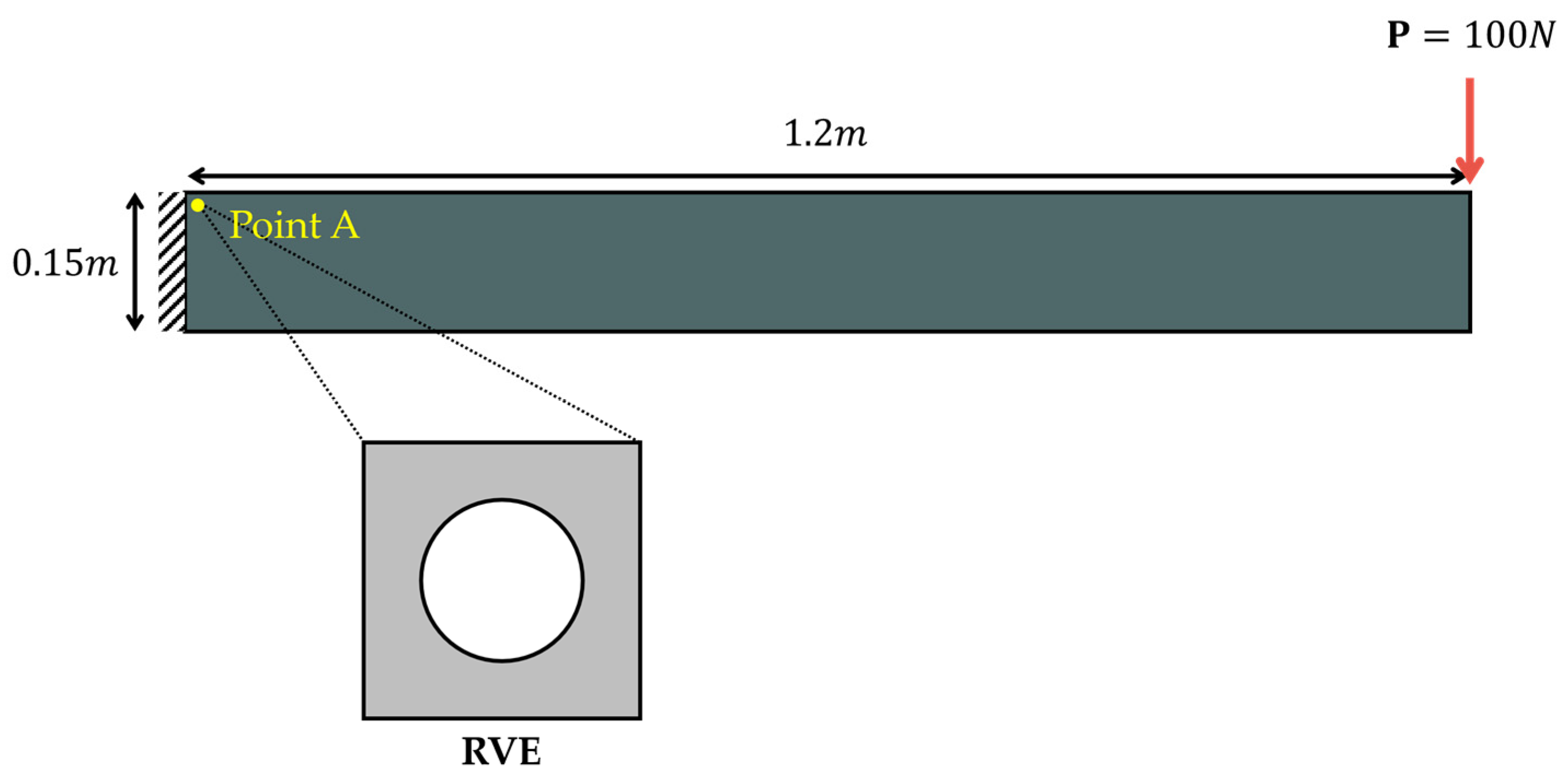
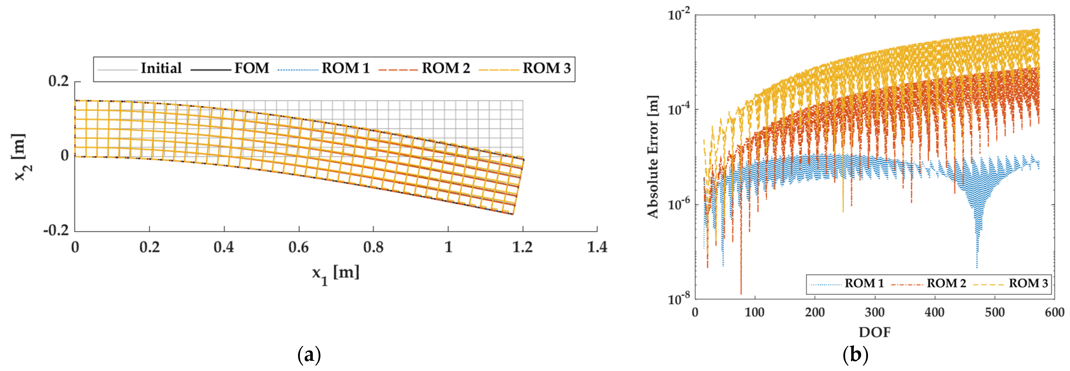
3.1. Example 1: Beam Model

As shown in Figure 2, a concentrated load $\mathbf{P}=-100 \mathrm{N}$ was applied to the top right edge of the beam consisting of a heterogeneous RVE model. We applied fixed boundary conditions for the left side of the beam. For finite element analysis, we constructed a macroscopic model using 240 elements and 287 nodes and an RVE model using 440 elements and 484 nodes. The material constants of the RVE model were $A_{10}=0.18 \mathrm{M}\mathrm{P}\mathrm{a}$ and $A_{01}=0.08 \mathrm{M}\mathrm{P}\mathrm{a}$.

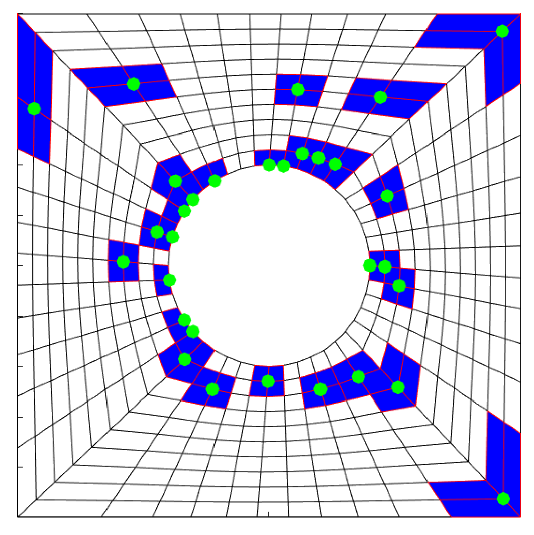
3.1.1. Construction of a Microscopic ROM (ROM1)

This subsection describes a procedure for generating the ROM of the RVE model. During the convergence process for simulating the nonlinear behaviors of the macroscopic model, strains change as they depend on the current state of the deformation. Since the RVE model is affected by the change of the macroscopic strain in the FE² procedure, we should construct the ROM of the RVE corresponding to various deformations. Therefore, we performed a priori parametric study on the macroscopic strain $\mathit{E}=\left(E_{xx},E_{yy},E_{xy}\right)$ within the range of $\left[-0.025\le \mathbf{E}\le 0.025\right]$ in the offline stage; the sample parameter values are shown in

Table 1. Information on sample parameters for constructing microscopic ROM.

${\mathit{n}}_{\mathit{p}}$	${\mathit{E}}_{\mathit{x}\mathit{x}}$	${\mathit{E}}_{\mathit{y}\mathit{y}}$	${\mathit{E}}_{\mathit{x}\mathit{y}}$
1	−0.025	−0.025	−0.025
2	0.025	−0.025	−0.025
3	−0.025	0.025	−0.025
4	0.025	0.025	−0.025
5	−0.025	−0.025	0.025
6	0.025	−0.025	0.025
7	−0.025	0.025	0.025
8	0.025	0.025	0.025

. Since the constructed ROM globally covers the range of macroscopic strains, the selected DEIM points and associated ROMs do not change during the entire FE² analysis (see Refs. [46,47] for the construction of local ROMs). At this stage, we did not conduct the FE² analysis, but we generated a snapshot matrix for all the iteration results of displacements and loads for the sample parameters from the microscopic nonlinear analysis. Then, we constructed a microscopic ROM using the POD-DEIM described in Section 2.2 and the generated data.

Information on the ROM is shown in

Table 2. Model information for microscopic FOM and ROM of example 1.

	FOM	ROM 1
# of DOFs	968	-
# of elements	440	87
# of bases	-	32
# of sample points	-	32

and Figure 3. The ‘#’ sign inside the table indicates a number. As shown in Table 2, the size of the reduced RVE model is about 3.3% compared with that of the FOM. In Figure 3, the green points are the ones selected for the DEIM interpolation by Algorithm 1, and the blue elements with red edge line represent the ones that contain the nodes of the DEIM points. We considered only the blue sample elements in the online stage out of the full elements.

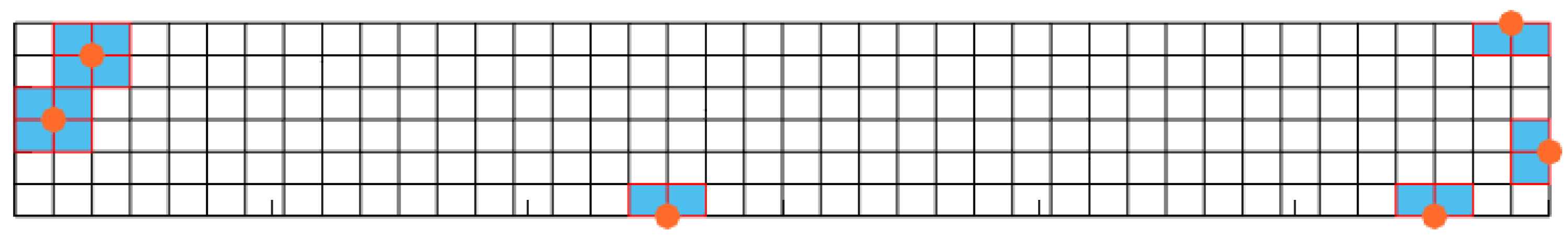
3.1.2. Construction of a Macroscopic ROM (ROM 2)

In the nonlinear FE² analysis, we performed a one-time FE² analysis to construct a macroscopic ROM since the RVE model determines the material properties (tangent moduli and stress) of the macroscopic model. In the offline stage, we generated the snapshot matrix for displacement and force through a full FE² analysis. Then, we constructed the macroscopic ROM by applying the POD-DEIM in Section 2.2.

Table 3. Model information for macroscopic FOM and ROM of example 1.

	FOM	ROM 2
# of DOFs	574	-
# of elements	240	16
# of bases	-	6
# of sample points	-	6

shows information on the FOM and ROM. The size of the ROM is about 1% of that of the FOM. Figure 4 is the DEIM points and elements selected by Algorithm 1. The orange points are the ones for the interpolation, and the sky-blue square of red edge line represents the sample element associated with the orange points. In the online stage, we computed only 16 sample elements out of 240.

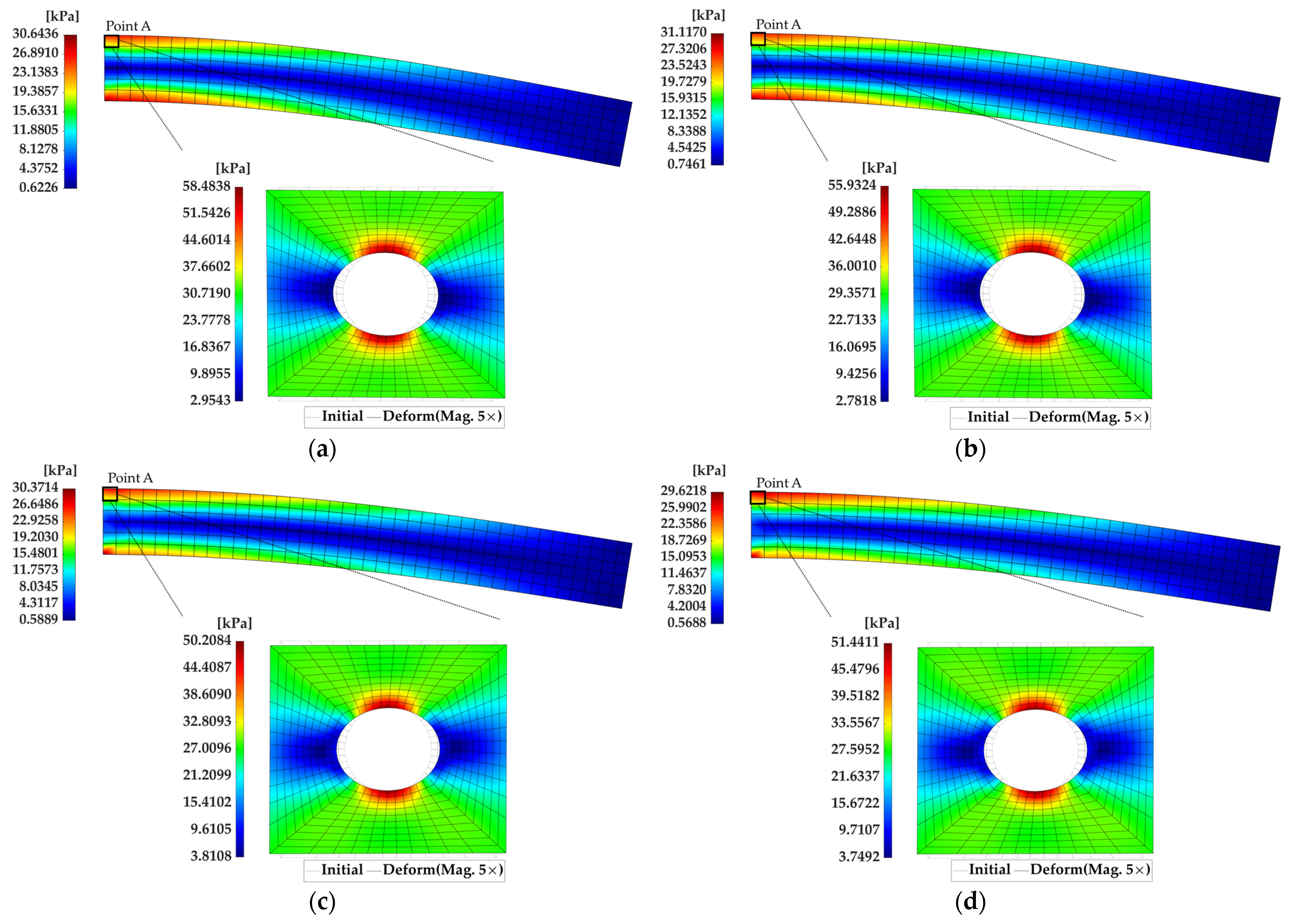
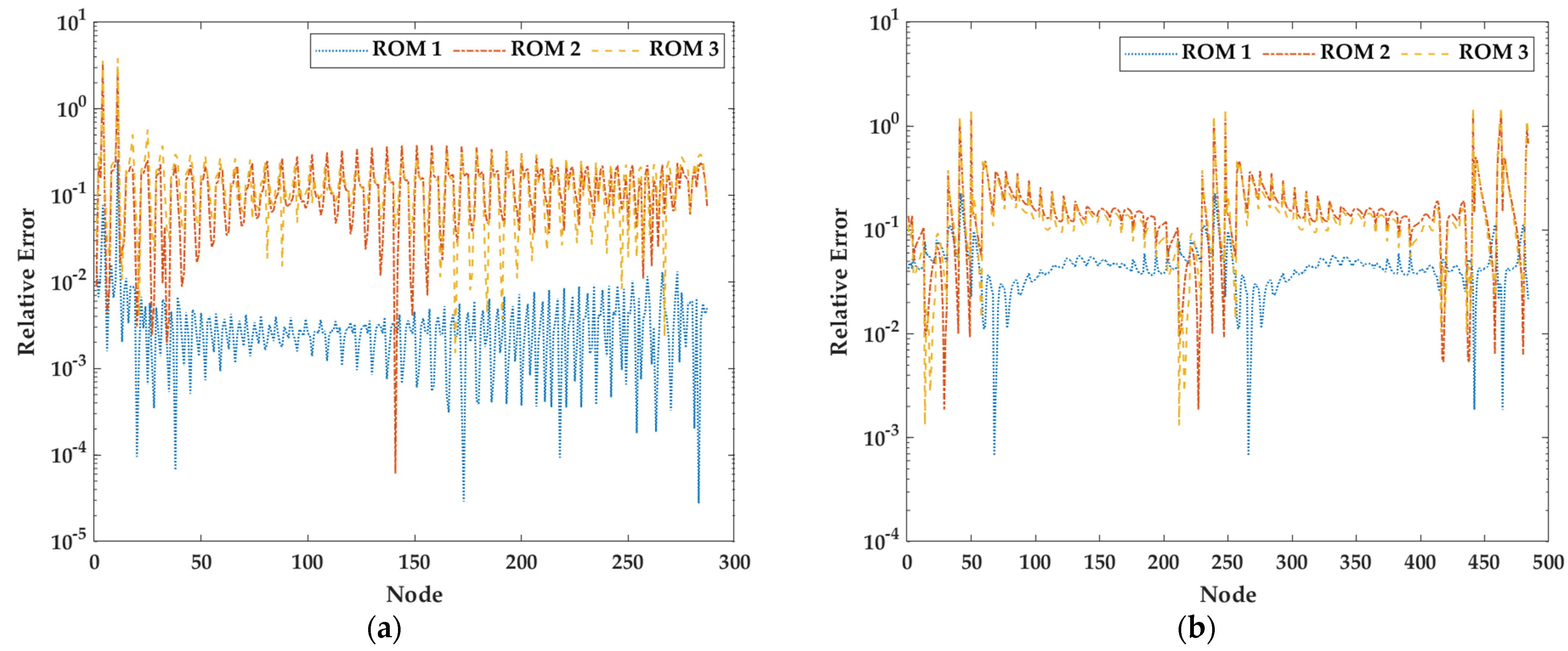
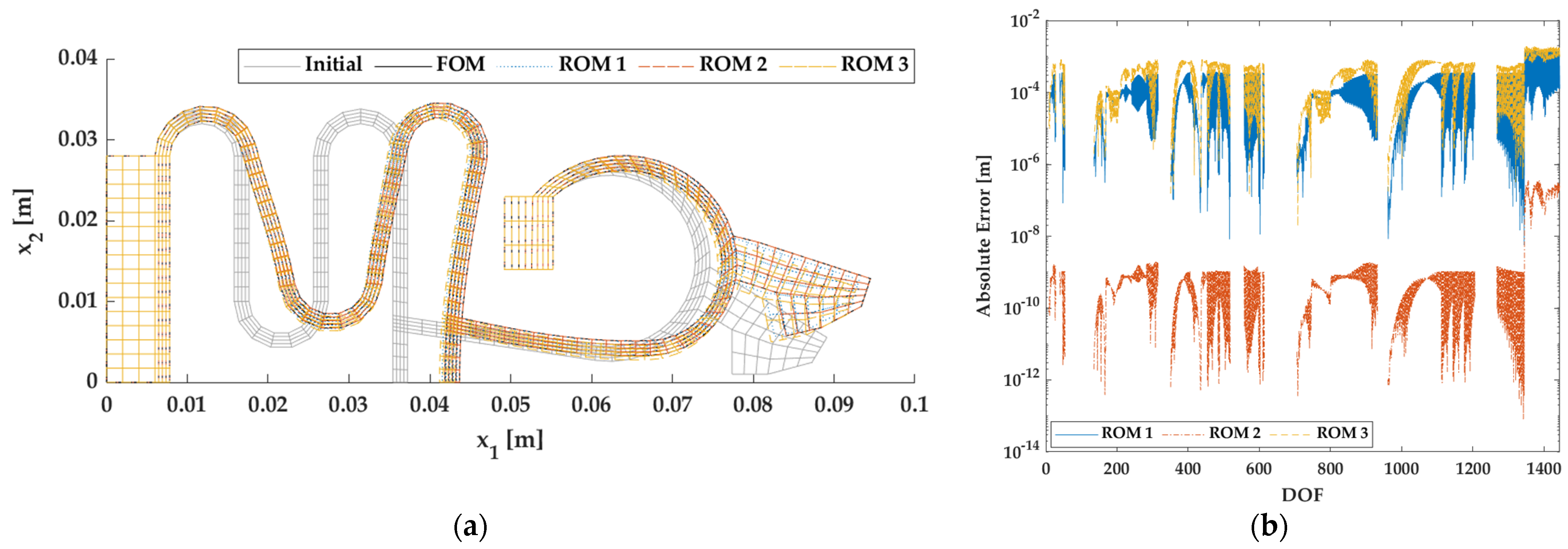
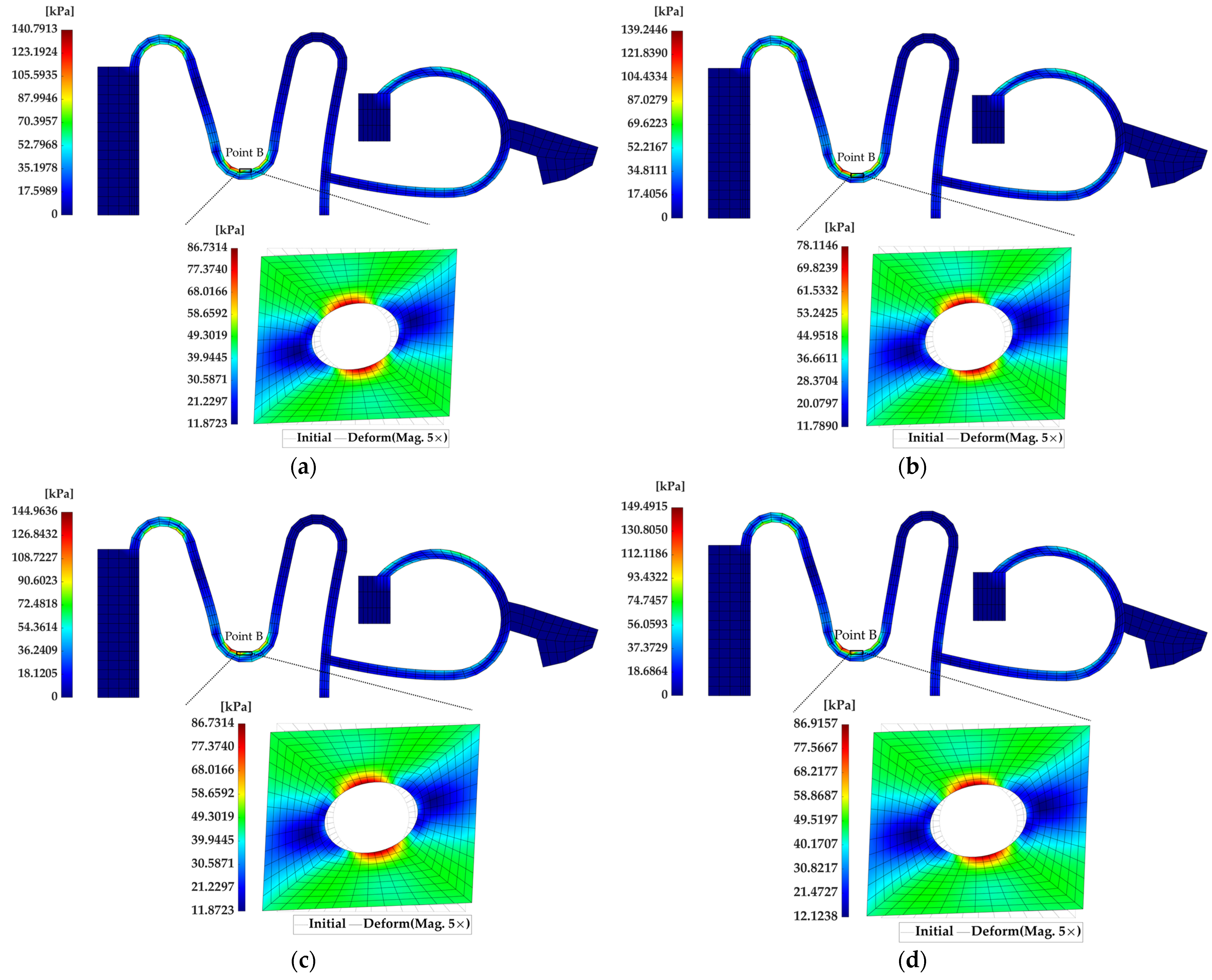
3.1.3. Results of FE² Analysis Using ROMs

We performed FE² analysis using ROMs, and we compared the classical FE² analysis (FOM) results to verify the accuracy and efficiency of the proposed ROM. Figure 5 shows the results of the deformation of the beam and absolute errors of all degrees of freedom (DOFs). ROM 3 is the one proposed in this work, which is a combination of ROM 1 and ROM 2. The ROMs were approximated within absolute errors of 10⁻⁶ to 10⁻², and ROM 1 showed the highest accuracy. Figure 6 presents the distribution of the von Mises stress. Like the von Mises stress distribution of the macroscopic domain, the von Mises stress distribution of the RVE model indicates similar results to the FOM. As shown in Figure 7, the ROMs have relative errors of less than 3.8 and 1.6 in the macroscopic and microscopic domains, respectively. We also compared the CPU time of the ROMs, as shown in

Table 4. Comparison of computation time for FE² analysis of example 1.

	FOM	ROM 1	ROM 2	ROM 3
Offline stage [h]	-	0.29	230	230.29
Online stage [h]	230	111.86	24.53	11.6

. The time to perform in Section 3.1.1 and Section 3.1.2 corresponds to the offline stage time of ROM 1 and ROM 2, respectively, and the online stage time is the actual computation time for performing FE² analysis using each ROM. From the viewpoint of efficiency in the online stage, the computation time of ROM 1 was about 2 times faster than the FOM, and ROM 2 was about 9.4 times faster than the FOM. ROM 3 is about 20 times faster than the FOM. Although the accuracy of ROM 3 is lower than ROM 1 and ROM 2, it shows the highest computational efficiency compared with the others.

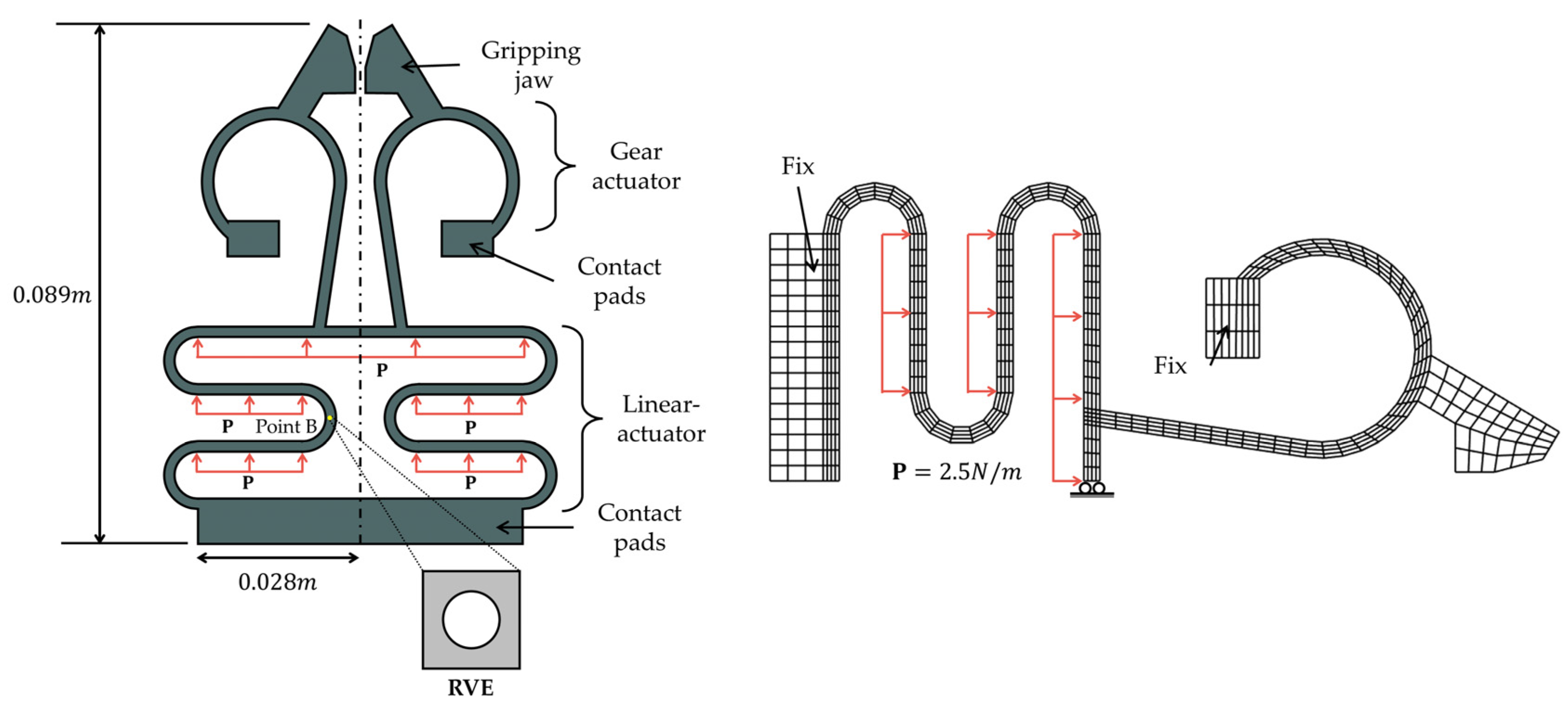
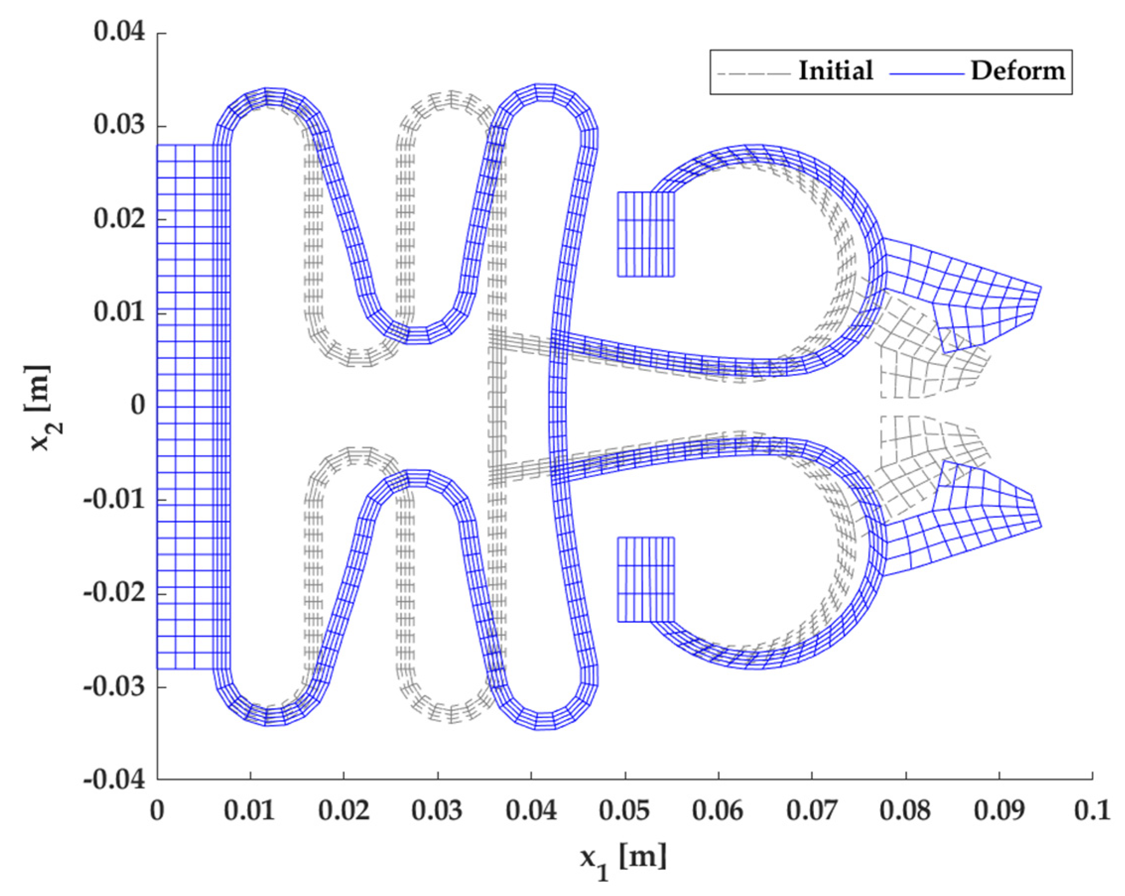
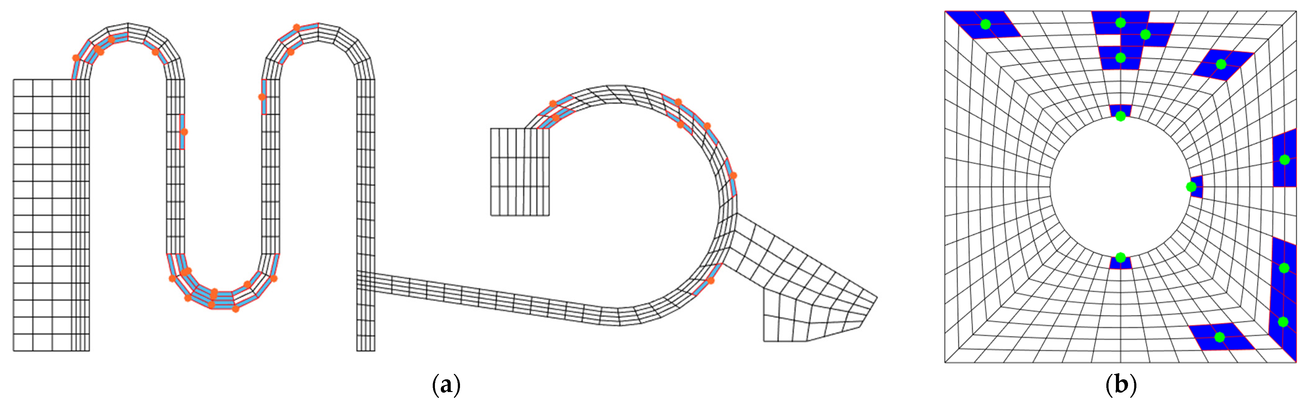
3.2. Example 2: Microgripper Model

The second example is a microgripper model [48] with a load applied at the linear actuator surface, as illustrated in Figure 8. When a load is applied to the microgripper, the gripping jaws open, and the microgripper is ready to grab an object. Due to the symmetry with respect to the horizontal axis in Figure 9, we considered only half of the macroscopic domain in the FE² analysis. The contact pads applied fixed boundary conditions. The macroscopic model consists of 579 elements and 722 nodes, and the RVE model has 432 elements and 480 nodes. In this example, the material constants of the RVE model were $A_{10}=\mathrm{333,900} \mathrm{P}\mathrm{a}$ and $A_{01}=-337 \mathrm{P}\mathrm{a}$, which are referenced from [7]. We performed the computations of this example using a parallel computing process in MATLAB.

To construct ROMs, we applied the same procedure as in example 1 in the offline stage. The sample parameters for the parametric study of the RVE model are also the same as Table 1. The ROMs information is shown in

Table 5. Model information for ROMs of example 2.

	ROM 1	ROM 2
# of elements	41	53
# of bases	13	27
# of sample points	13	27

and Figure 10. Table 5 shows the information on the system size for the macro- and microscopic ROMs. Figure 10 plots the location information of the selected point applying the DEIM. In Figure 10a, which is the macroscopic ROM information, the orange points are the DEIM points, and the sky-blue square of red edge line represents the sample element associated with the orange points. In Figure 10b, which is the microscopic ROM information, the green points are the DEIM points, and the blue square of red edge line represents the sample element. The ROM 1 and ROM 2 have about 1.4% and 1.9% of the size of the FOM, respectively.

In Figure 11, the deformation of the microgripper after FE² analysis was plotted by comparing the FOM and ROMs and the absolute errors of the displacement of all DOFs. The ROMs show similar results to those of the FOM within the absolute error range of 10⁻⁸ to 10⁻³. The ROM 2 shows the highest accuracy in this example. Comparing the macroscopic deformations of each example presented in Figure 5b and Figure 11b, whereas reducing the microscopic problem does not cause much decrease in accuracy in the case of example 1, the situation is flipped for example 2, as the overall macroscopic behavior of example 1 is simpler compared to that of example 2. In other words, although the accuracy of the ROM3 is inferior to that of ROM1, it is natural, as the online efficiency of the ROM3 is superior to that of the other ROMs. Revealing the tendency of the accuracy–efficiency tradeoff for the FE² procedure needs to be further investigated in the future.

Figure 12 presents the distribution of the von Mises stress. As per the von Mises stress distribution of the macroscopic domain, the von Mises stress distribution of the RVE model indicates similar results to the FOM. As illustrated in Figure 13, the ROMs exhibit a relative error of less than 3.2 and 0.14 in the macroscopic and microscopic domains, respectively.

Regarding the efficiency evaluation of the proposed method,

Table 6. Comparison of computation time for FE² analysis of example 2.

	FOM	ROM 1	ROM 2	ROM 3
Offline stage [h]	-	0.04	18.42	18.46
Online stage [h]	18.42	3.24	2.96	0.80

represents the computation time of each model. The online computation time of ROM 1 was about 5.7 times faster than the FOM, and ROM 2 was about 6.2 times faster than the FOM. ROM 3 was about 23 times faster than the FOM. Whereas ROM 3 has similar accuracy to ROM 1, it shows the highest computational efficiency among the ROMs. Figure 14 compares the CPU time of each ROM, including the offline stage. Although ROM 1 shows much less offline time than ROM 2 and 3, its applicability is limited to a single RVE model, and the online efficiency is not more competitive than the others. ROM 3 shows the highest efficiency, but it could be less accurate than the other two ROMs because the data loss is greater. In particular, ROM 2 is more efficient than ROM 1 from an online stage perspective. However, since at least one full FE² analysis is required to build ROM 2, the computational cost of the offline stage is high. Considering that the proposed method can be extended to a parametric ROM, which was extensively investigated for various linear ROMs with large-scale systems [49,50] and actively extended to nonlinear models [51,52], ROM 3 is the most appropriate compared to the other two ROMs since its online efficiency is superior to achieve a real-time, or near real-time, performance.

4. Conclusions

In this study, we proposed a new model order reduction method for efficient nonlinear FE² analysis by applying hyper-reduction to both micro- and macroscale problems. As investigated in the numerical example section, a conventional nonlinear FE² analysis requires a lot of computational resources as it performs two-scale analyses sequentially and concurrently. Therefore, the model order reduction technique is one of the most useful methods to resolve this issue. In general, the model order reduction method process is divided into an offline stage to obtain the FOM data for building an ROM and an online stage to derive a response using the constructed ROM. We mainly focused on enhancing the online efficiency that usually suffers from repetitive computations, considering the nonlinearities of the materials and structures.

While previous studies aimed to reduce the computation time of the microscopic ROM of the RVE model to increase efficiency, the present work focused on guaranteeing efficiency by reducing the number of operations of the RVE model using the macroscopic ROM. With a reduced number of elements to be evaluated in the macroscopic problem, the number of evaluations of the microscopic model was also decreased, realizing an overall reduction in the computations in the FE² analysis. As a result, the online efficiency is greatly enhanced compared with the previous ROM, which only applied the ROM to microscopic problems. Although the offline cost is relatively higher than the previous ROM, it is incurred once and could be further reduced through future improvements such as multi-fidelity [53,54]. This study is significant in that it suggests a new direction for improving the efficiency of concurrent nonlinear FE² analysis by reducing the number of microscale problem evaluations. The proposed method has the potential to serve as a surrogate model within a direct FE² analysis, which has a similar framework to classical FE².

For further development, parametric ROMs could be one of the major topics, not simply by repeating the proposed method within a parametric domain of interest, but by developing an efficient strategy that minimizes the number of sparse elements in both scales.

References

1. Uchida, M.; Kaneko, Y. Nonlocal multiscale modeling of deformation behavior of polycrystalline copper by second-order homogenization method. Eur. Phys. J. B 2019, 92, 189. [Google Scholar] [CrossRef]
2. Bleiler, C.; Castañeda, P.P.; Röhrle, O. Tangent second-order homogenisation estimates for incompressible hyperelastic composites with fibrous microstructures and anisotropic phases. J. Mech. Phys. Solids 2021, 147, 104251. [Google Scholar] [CrossRef]
3. Kouznetsova, V.G.; Geers, M.G.; Brekelmans, W. Multi-scale second-order computational homogenization of multi-phase materials: A nested finite element solution strategy. Comput. Methods Appl. Mech. Eng. 2004, 193, 5525–5550. [Google Scholar] [CrossRef]
4. Matsui, K.; Terada, K.; Yuge, K. Two-scale finite element analysis of heterogeneous solids with periodic microstructures. Comput. Struct. 2004, 82, 593–606. [Google Scholar] [CrossRef]
5. Xu, R.; Yang, J.; Yan, W.; Huang, Q.; Giunta, G.; Belouettar, S.; Hu, H. Data-driven multiscale finite element method: From concurrence to separation. Comput. Methods Appl. Mech. Eng. 2020, 363, 112893. [Google Scholar] [CrossRef]
6. Feng, N.; Zhang, G.; Khandelwal, K. Finite strain FE2 analysis with data-driven homogenization using deep neural networks. Comput. Struct. 2022, 263, 106742. [Google Scholar] [CrossRef]
7. Kim, S.; Shin, H. Deep learning framework for multiscale finite element analysis based on data-driven mechanics and data augmentation. Comput. Methods Appl. Mech. Eng. 2023, 414, 116131. [Google Scholar] [CrossRef]
8. Kim, S.; Shin, H. Data-driven multiscale finite-element method using deep neural network combined with proper orthogonal decomposition. Eng. Comput. 2024, 40, 661–675. [Google Scholar] [CrossRef]
9. Tan, V.B.C.; Raju, K.; Lee, H.P. Direct FE2 for concurrent multilevel modelling of heterogeneous structures. Comput. Methods Appl. Mech. Eng. 2020, 360, 112694. [Google Scholar] [CrossRef]
10. Xu, J.; Li, P.; Poh, L.H.; Zhang, Y.; Tan, V.B.C. Direct FE2 for concurrent multilevel modeling of heterogeneous thin plate structures. Comput. Methods Appl. Mech. Eng. 2022, 392, 114658. [Google Scholar] [CrossRef]
11. Liu, K.; Meng, L.; Zhao, A.; Wang, Z.; Chen, L.; Li, P. A hybrid direct FE2 method for modeling of multiscale materials and structures with strain localization. Comput. Methods Appl. Mech. Eng. 2023, 412, 116080. [Google Scholar] [CrossRef]
12. Liu, K.; Tian, L.; Gao, T.; Wang, Z.; Li, P. An explicit D-FE2 method for transient multiscale analysis. Int. J. Mech. Sci. 2025, 285, 109808. [Google Scholar] [CrossRef]
13. Cremonesi, M.; Néron, D.; Guidault, P.A.; Ladevèze, P. A PGD-based homogenization technique for the resolution of nonlinear multiscale problems. Comput. Methods Appl. Mech. Eng. 2013, 267, 275–292. [Google Scholar] [CrossRef]
14. El Halabi, F.; González, D.; Chico, A.; Doblaré, M. FE2 multiscale in linear elasticity based on parametrized microscale models using proper generalized decomposition. Comput. Methods Appl. Mech. Eng. 2013, 257, 183–202. [Google Scholar] [CrossRef]
15. Yvonnet, J.; Zahrouni, H.; Potier-Ferry, M. A model reduction method for the post-buckling analysis of cellular microstructures. Comput. Methods Appl. Mech. Eng. 2007, 197, 265–280. [Google Scholar] [CrossRef]
16. Oliver, J.; Caicedo, M.; Huespe, A.E.; Hernández, J.A.; Roubin, E. Reduced order modeling strategies for computational multiscale fracture. Comput. Methods Appl. Mech. Eng. 2017, 313, 560–595. [Google Scholar] [CrossRef]
17. Carlberg, K.; Farhat, C.; Cortial, J.; Amsallem, D. The GNAT method for nonlinear model reduction: Effective implementation and application to computational fluid dynamics and turbulent flows. J. Comput. Phys. 2013, 242, 623–647. [Google Scholar] [CrossRef]
18. Kerfriden, P.; Goury, O.; Rabczuk, T.; Bordas, S.P.A. A partitioned model order reduction approach to rationalise computational expenses in nonlinear fracture mechanics. Comput. Methods Appl. Mech. Eng. 2013, 256, 169–188. [Google Scholar] [CrossRef]
19. Raschi, M.; Lloberas-Valls, O.; Huespe, A.; Oliver, J. High performance reduction technique for multiscale finite element modeling (HPR-FE2): Towards industrial multiscale FE software. Comput. Methods Appl. Mech. Eng. 2021, 375, 113580. [Google Scholar] [CrossRef]
20. Lee, J.; Park, Y.; Lee, J.; Cho, M. Non-intrusive reduced-order modeling for nonlinear structural systems via radial basis function-based stiffness evaluation procedure. Comput. Struct. 2024, 304, 107500. [Google Scholar] [CrossRef]
21. Lee, J.; Lee, J.; Cho, H.; Kim, E.; Cho, M. Reduced-order modeling of nonlinear structural dynamical systems via element-wise stiffness evaluation procedure combined with hyper-reduction. Comput. Mech. 2021, 67, 523–540. [Google Scholar] [CrossRef]
22. Van Tuijl, R.A.; Remmers, J.J.; Geers, M.G. Integration efficiency for model reduction in micro-mechanical analyses. Comput. Mech. 2018, 62, 151–169. [Google Scholar] [CrossRef] [PubMed]
23. An, S.S.; Kim, T.; James, D.L. Optimizing cubature for efficient integration of subspace deformations. ACM Trans. Graph. 2008, 27, 1–10. [Google Scholar] [CrossRef]
24. Hernández, J.A.; Caicedo, M.A.; Ferrer, A. Dimensional hyper-reduction of nonlinear finite element models via empirical cubature. Comput. Methods Appl. Mech. Eng. 2017, 313, 687–722. [Google Scholar] [CrossRef]
25. Lange, N.; Hütter, G.; Kiefer, B. A monolithic hyper ROM FE2 method with clustered training at finite deformations. Comput. Methods Appl. Mech. Eng. 2024, 418, 116522. [Google Scholar] [CrossRef]
26. Giuliodori, A.; Hernández, J.A.; Soudah, E. Multiscale modeling of prismatic heterogeneous structures based on a localized hyperreduced-order method. Comput. Methods Appl. Mech. Eng. 2023, 407, 115913. [Google Scholar] [CrossRef]
27. Hernández, J.A. A multiscale method for periodic structures using domain decomposition and ECM-hyperreduction. Comput. Methods Appl. Mech. Eng. 2020, 368, 113192. [Google Scholar] [CrossRef]
28. Guo, T.; Rokoš, O.; Veroy, K. A reduced order model for geometrically parameterized two-scale simulations of elasto-plastic microstructures under large deformations. Comput. Methods Appl. Mech. Eng. 2024, 418, 116467. [Google Scholar] [CrossRef]
29. Rocha, I.B.; Kerfriden, P.; van der Meer, F.P. Micromechanics-based surrogate models for the response of composites: A critical comparison between a classical mesoscale constitutive model, hyper-reduction and neural networks. Eur. J. Mech. A/Solids 2020, 82, 103995. [Google Scholar] [CrossRef]
30. Ghavamian, F.; Tiso, P.; Simone, A. POD-DEIM model order reduction for strain-softening viscoplasticity. Comput. Methods Appl. Mech. Eng. 2017, 317, 458–479. [Google Scholar] [CrossRef]
31. Tiso, P.; Rixen, D.J. Discrete Empirical Interpolation Method for Finite Element Structural Dynamics. In Proceedings of the 31st IMAC A Conference on Structural Dynamics, Garden Grove, CA, USA, 11–14 February 2013. [Google Scholar] [CrossRef]
32. Carlberg, K.; Tuminaro, R.; Boggs, P. Preserving Lagrangian structure in nonlinear model reduction with application to structural dynamics. SIAM J. Sci. Comput. 2015, 37, B153–B184. [Google Scholar] [CrossRef]
33. Carlberg, K.; Tuminaro, R.; Boggs, P. Efficient structure-preserving model reduction for nonlinear mechanical systems with application to structural dynamics. In Proceedings of the 53rd AIAA/ASME/ASCE/AHS/ASC Structures, Structural Dynamics and Materials Conference, Honolulu, HI, USA, 23–26 April 2012. [Google Scholar] [CrossRef]
34. Bonomi, D.; Manzoni, A.; Quarteroni, A. A Matrix DEIM Technique for Model Reduction of Nonlinear Parametrized Problems in Cardiac Mechanics. Comput. Methods Appl. Mech. Eng. 2017, 324, 300–326. [Google Scholar] [CrossRef]
35. Chaturantabut, S.; Sorensen, D.C. Nonlinear model reduction via discrete empirical interpolation. SIAM J. Sci. Comput. 2010, 32, 2737–2764. [Google Scholar] [CrossRef]
36. Soldner, D.; Brands, B.; Zabihyan, R.; Steinmann, P.; Mergheim, J. Computational Homogenisation using Reduced-Order Modelling applied to Hyperelasticity. In Proceedings of the Applied Mathematics and Mechanics, Braunschweig, Germany, 7–11 March 2016. [Google Scholar] [CrossRef]
37. Soldner, D.; Brands, B.; Zabihyan, R.; Steinmann, P.; Mergheim, J. A numerical study of different projection-based model reduction techniques applied to computational homogenisation. Comput. Mech. 2017, 60, 613–625. [Google Scholar] [CrossRef]
38. Hill, R. Elastic properties of reinforced solids: Some theoretical principles. J. Mech. Phys. Solids 1963, 11, 357–372. [Google Scholar] [CrossRef]
39. Hill, R. On constitutive macro-variables for heterogeneous solids at finite strain. In Proceedings of the Royal Society of London A: Mathematical, Physical and Engineering Sciences; The Royal Society: London, UK, 1972. [Google Scholar] [CrossRef]
40. Hill, R. On macroscopic effects of heterogeneity in elastoplastic media at finite strain. In Mathematical Proceedings of the Cambridge Philosophical Society; Cambridge University Press: Cambridge, UK, 1984. [Google Scholar] [CrossRef]
41. Matouš, K.; Geers, M.G.; Kouznetsova, V.G.; Gillman, A. A review of predictive nonlinear theories for multiscale modeling of heterogeneous materials. J. Comput. Phys. 2017, 330, 192–220. [Google Scholar] [CrossRef]
42. Terada, K.; Kikuchi, N. A class of general algorithms for multi-scale analyses of heterogeneous media. Comput. Methods Appl. Mech. Eng. 2001, 190, 5427–5464. [Google Scholar] [CrossRef]
43. Barrault, M.; Maday, Y.; Nguyen, N.C.; Patera, A.T. An ‘empirical interpolation’ method: Application to efficient reduced-basis discretization of partial differential equations. Comp. Rendus Math. 2004, 339, 667–672. [Google Scholar] [CrossRef]
44. Radermacher, A.; Reese, S. POD-based model reduction with empirical interpolation applied to nonlinear elasticity. Int. J. Numer. Meth. Engng. 2015, 107, 407–495. [Google Scholar] [CrossRef]
45. Kim, N.H. Introduction to Nonlinear Finite Element Analysis; Springer: Berlin/Heidelberg, Germany, 2015; pp. 183–199. [Google Scholar] [CrossRef]
46. Amsallem, D.; Haasdonk, B. PEBL-ROM: Projection-error based local reduced-order models. Adv. Model. Simul. Eng. Sci. 2016, 3, 6. [Google Scholar] [CrossRef]
47. Cho, H.; Shin, S.; Kim, H.; Cho, M. Enhanced model-order reduction approach via online adaptation for parametrized nonlinear structural problems. Comput. Mech. 2020, 65, 331–353. [Google Scholar] [CrossRef]
48. Kohl, M.; Krevet, B.; Just, E. SMA microgripper system. Sens. Actuators A Phys. 2002, 97, 646–652. [Google Scholar] [CrossRef]
49. Cheon, S.; Lee, J. An enhanced hybrid-level interface-reduction method combined with an interface discrimination algorithm. Mathematics 2023, 11, 4867. [Google Scholar] [CrossRef]
50. Cheon, S.; Lee, S.; Lee, J. A system-level interface sampling and reduction method for component mode synthesis with varying parameters. Appl. Math. Comput. 2024, 476, 128778. [Google Scholar] [CrossRef]
51. Bhattacharya, K.; Hosseini, B.; Kovachki, N.B.; Stuart, A.M. Model reduction and neural networks for parametric PDEs. SMAI J. Comput. Math. 2021, 7, 121–157. [Google Scholar] [CrossRef]
52. Touzé, C.; Vizzaccaro, A.; Thomas, O. Model order reduction methods for geometrically nonlinear structures: A review of nonlinear techniques. Nonlinear Dyn. 2021, 105, 1141–1190. [Google Scholar] [CrossRef]
53. Kast, M.; Guo, M.; Hesthaven, J.S. A non-intrusive multifidelity method for the reduced order modeling of nonlinear problems. Comput. Methods Appl. Mech. Eng. 2020, 364, 112947. [Google Scholar] [CrossRef]
54. Conti, P.; Guo, M.; Manzoni, A.; Frangi, A.; Brunton, S.L.; Nathan Kutz, J. Multi-fidelity reduced-order surrogate modelling. Proc. R. Soc. A 2024, 480, 20230655. [Google Scholar] [CrossRef]
Figure 1. Illustration of FE2 method.
Mathematics 13 01790 g001
Figure 2. Example 1: beam model with a clamped end.
Mathematics 13 01790 g002
Figure 3. Location of DEIM points and associated elements selected by Algorithm 1 for the RVE model.
Mathematics 13 01790 g003
Figure 4. Location of DEIM points and associated elements selected by Algorithm 1 for the macroscopic domain.
Mathematics 13 01790 g004
Figure 5. Results of beam model using ROMs: (a) deformation of FOM and ROMs; (b) absolute error of displacement depending on all DOFs.
Mathematics 13 01790 g005
Figure 6. Distribution of macroscopic von Mises stress and microscopic von Mises stress at point A: (a) FOM; (b) using ROM 1; (c) using ROM 2; (d) using ROM 3.
Mathematics 13 01790 g006
Figure 7. Relative error of von Mises stress depending on all nodes: (a) macroscopic; (b) microscopic at point A.
Mathematics 13 01790 g007
Figure 8. Example 2: microgripper model.
Mathematics 13 01790 g008
Figure 9. Deformation of microgripper model.
Mathematics 13 01790 g009
Figure 10. Locations of DEIM points and associated elements of example 2: (a) macroscopic ROM; (b) microscopic ROM.
Mathematics 13 01790 g010
Figure 11. Results of microgripper model using ROMs: (a) deformation of FOM and ROMs; (b) absolute error.
Mathematics 13 01790 g011
Figure 12. Distribution of macroscopic von Mises stress and microscopic von Mises stress at point B: (a) FOM; (b) using ROM 1; (c) using ROM 2; (d) using ROM 3.
Mathematics 13 01790 g012
Figure 13. Relative error of von Mises stress depending on all nodes: (a) macroscopic; (b) microscopic at point B.
Mathematics 13 01790 g013
Figure 14. Comparison of the computation time: (a) example 1; (b) example 2.
Mathematics 13 01790 g014