Abstract
In this study, the extended finite element method (XFEM) was integrated into the generalized multiscale finite element method with global–local enrichment (GFEMgl) to simulate 2D heat conduction in highly heterogeneous materials (i.e., matrixes with numerous randomly distributed inclusions or voids). This multiscale scheme was used to evaluate the effective thermal conductivity (ETC) of composites through simulation based on a representative volume element (RVE). In the proposed method, global–local enrichments are numerically constructed and incorporated into the global approximation in a hierarchical manner to integrate microstructure information into the macroscale problem. The XFEM is employed on a microscale mesh to avoid using a conformal mesh. RVEs containing numerous inclusions or voids with different volume fractions were numerically simulated using the proposed multiscale method, and the obtained results were compared with those of the standard single-scale XFEM and analytical models. The simulation results indicated that the proposed method has excellent accuracy and considerably lower computational cost.
MSC:
35-04
1. Introduction
There has been increasing interest in multi-phase composite materials as structure materials in recent years because some of their physical performance can be tailored by changing the volume fraction of constituents [1]. These heterogeneous structures can be produced through additive manufacturing, 3D printing, or irradiation. In the heat transfer problem, the presence of heterogeneity impedes or diverts heat flow and can affect overall and local material behavior. The effective thermal conduction of composite materials is a key parameter in numerous engineering applications, including those related to building insulation material, nuclear fuel components, microelectronic packaging, and aircraft thermal barriers. The accurate prediction of thermal stress highly depends on the precise prediction of both global and local temperature distributions.
Effective thermal conductivity (ETC) reflects the macroscopic heat transfer property according to the Fourier law. Accurately determining the ETC of a composite material is critical for performing heat conduction simulations for large-scale structures. By optimizing the thermal conductivity modeling of composite materials, it is possible to develop materials with excellent thermal properties. For example, by incorporating nanofillers (such as alumina or boron nitride) into polymer matrices, lightweight and highly efficient thermal insulating materials can be designed. These materials can be used in building exterior walls, roof insulation layers, and other applications to enhance the energy efficiency of buildings.
Various analytical equations have been developed for evaluating the ETC of heterogeneous media. Many ETC models found in the literature are based on the five structural models: the boundary parallel-series (PS) model [2], Maxwell–Eucken model [3], Hashin–Shtrikman model [4], effective medium theory (EMT) model [5], and Johansen geometric average model [6]. A review of many analytical models can also be found in Ref. [7]. However, in most analytical expressions, ETC is a direct function of the thermal conductivities of phases and their volume fraction; such models do not capture the complexity of ETC, which is significantly affected by the local arrangement of these phases.
Numerical simulation of the heat transfer problem can provide detailed field variables in composite materials; many numerical methods have been developed to predict the ETC in composites, including the finite element method (FEM) [8], boundary element method (BEM) [9], and lattice Boltzmann method (LBM) [10]. With FEM-based commercial software being available, FEM is the standard choice for calculating the ETC of composites. For example, Shen et al. [11] numerically simulated the heat transfer in porous microstructures with periodically arranged pores, and their numerical models could be simplified into unit cells. Ziwei Li et al. [12] conducted FEM analyses for unit Kelvin cells to examine the steady heat transfer in composite lattice-based materials. The LBM has advantages in easy implementation and handling complex geometries and, therefore, has already been applied to various types of composites such as granular materials, hierarchical porous structures, and fiber-reinforced media. However, LBM-based simulation requires extensive computational cost. The existing literature on numerical simulation has mainly focused on composites with periodical or symmetrical structures and numerical analyses of heterogeneous materials, while randomly distributed constituents have rarely been reported.
The extended finite element method (XFEM) was first proposed to solve fracture mechanics problems but was later extensively used to model many types of discontinuities in solid mechanics, such as inclusions and voids [13], cohesive cracks [14], heterogeneous materials [15], and delamination propagation [16]. In this method, pre-tailored functions are introduced to enrich the FEM approximation of displacement fields based on partition of unity. Therefore, the discontinuities can be modeled on a structured mesh, without requiring that the mesh conforms to these physical boundaries. The XFEM has been applied for simulation of temperature fields. For example, T.T. Yu et al. [17] applied the XFEM to simulate unsteady temperature fields in heterogeneous materials, where level-set-based enrichment functions are employed to model material interfaces. Thermal fracture analyses by the XFEM have also become more common. Zamani et al. [18] first implemented the XFEM to study a homogeneous medium containing a stationary crack under thermal load. Later, the XFEM was used for dynamic analyses of stationary and moving cracks in a two-dimensional homogeneous medium under thermal shock. Then, stress intensity factors (SIFs) were computed for fatigue life evaluation [19]. Although the XFEM solves some challenges associated with meshing, accurately determining ETC requires numerous inclusions or pores to be included in the concept of representative volume elements (RVEs); a full-scale analysis of such a domain consumes enormous degrees of freedom and a tremendous amount of computational processing unit (CPU) time.
To reduce the computation costs, many multiscale methods have been proposed for highly heterogeneous materials and have become increasingly popular. The first kind of methods are asymptotic homogenization-based methods such as the stochastic homogenization approach [20] and multiscale aggregating approach [21]. In these methods, the FEM is employed at certain points to estimate the homogenized material properties and, in turn, is used for simulation of the bulk structure. These methods typically are applicable to periodic materials and only provide overall responses of the bulk structure. The other kind of methods are called concurrent multiscale methods, which enable scale separation by space decomposition and bridging, such as the variational multiscale method (VMM) [22,23], domain decomposition approach [24], multiscale finite element method (MsFEM) [25,26], and multiscale projection method [27]. These kinds of methods can provide detailed field information, both on a macroscale and microscale, but typically, iterative procedures between two scales are required, which increase the computational cost. Alternatively, multi-level adaptive refinement approaches were developed with the aid of variable-node elements; thus, problems with microstructures can be solved on a single-scale, highly refined mesh, such as VNE (variable-node element) [28], variable-node XFEM [29], and VP-XFEM (virtual-node-polygon element) [30].
Another major multiscale computational method is the generalized finite element method with global–local enrichment functions (GFEMgl), which is developed as a modification of the GFEM in Ref. [31]. The GFEM and XFEM are both based on partition of unity (PoU). If a priori knowledge is unavailable from any analytical solution, the enrichment functions can be obtained by solving the auxiliary local problems; the resulting local field will be used as global–local enrichments. These enrichment functions are incorporated into the FEM approximation in a hierarchical manner [32]. The method can be implemented on legacy FEM software programs by using non-intrusive algorithms, with no modifications to the FEM code required. This method has been applied to several multiscale problems, such as fracture mechanic problems [31,33], sharp thermal gradient [34], advection–diffusion problems [35], and multi-physics or non-linear problems [36,37]. To the best of the author’s knowledge, GFEMgl is mainly used to simulate localized phenomena. Considering the advantages of GFEMgl and XFEM, the development of a multiscale method which combines these two methods for the multiscale homogenization of composite materials is an attractive proposition.
The present study developed a novel numerical analysis method by combining the XFEM and GFEMgl to simulate 2D heat conduction in highly heterogeneous materials. In this novel proposed multiscale method, XFEM and level set functions are applied at the microscale level to avoid conformal meshing, and GFEMgl is used as a multiscale framework to enable scale separation. Moreover, shifted global–local enrichment functions are specially proposed to cope with boundary conditions in multiscale homogenization problems. These enrichment functions are numerically constructed by solving auxiliary local boundary value problems, and the XFEM is employed to model the inclusions or pores at the micro level. Finally, the enriched global problem is solved with such global–local enrichments added into the global approximation space in a hierarchical manner. Compared with existing numerical methods, the proposed multiscale method can obtain global and local responses with considerably fewer degrees of freedom and substantially less CPU time. The proposed method was used to solve steady 2D heat transfer problems and determine the ETC of the composites with numerous inclusions and pores which are assumed to be randomly distributed within each RVE. Note that, in our method, multiscale base functions are constructed by solving boundary value problems, which can be efficiently carried out in general commercial software. Therefore, the current method can be easily implemented in these software packages with little programming effort.
The rest of this paper is organized as follows. Section 2 presents the XFEM approximation of the temperature field in heterogeneous materials. Section 3 details the implementation process of the GFEMgl and the construction procedure for global–local enrichments and their shifted modification. Section 4 presents various numerical experiments to examine the effectiveness of the proposed method; this section also provides comparison between the results of the proposed method, single-scale XFEM, and analytical models. Finally, Section 5 presents some concluding remarks of this study.
2. XFEM Model of Temperature Fields
2.1. Mathematical Formulation of XFEM
In this study, XFEM was implemented at the microscale level to avoid a conformal mesh. In the XFEM, a structured mesh is generated without consideration of the physical boundaries of the discontinuities. Then, analytically defined enrichment functions are incorporated into the FEM approximation to model discontinuities based on PoU. For detailed derivations of the XFEM approximation and the concept of PoU, readers can refer to the classic literature [13,14,15,16]. The XFEM approximation function of a temperature field containing inclusions can be expressed as follows:
where denotes the collection of all nodes in the domain, represents the nodal temperature, and is a standard FE shape function. is the set of nodes whose support intersects with the material interfaces as shown in Figure 1, is the shape functions reproducing the enrichment that can differ from , is enriched nodal variables associating with the nodes , and is the enrichment function.
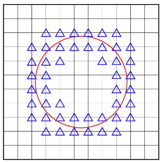
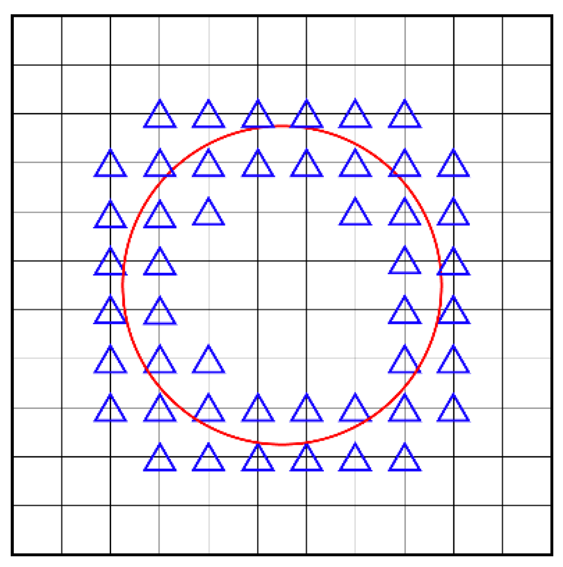
Figure 1.
The XFEM enrichment scheme for one circular inclusion (red line) within the domain. Nodes marked with blue triangulars are enriched by .
The enrichment function used for modeling material interfaces has the following form:
where is a signed distance level set function, which is used to numerically describe the interface. And it can be defined as follows.
where, represents the normal projection of the point onto the interface , and is the normal vector to the interface at the point . This level set function is positive on one side of the discontinuity and negative on the other side. On the interface, .
For voids modeling, the XFEM approximation of the temperature field can be expressed as follows:
where the void enrichment function is assigned a value of 0 inside the void and 1 anywhere else. Furthermore, nodes whose supports are completely within the void are associated with a fixed degree of freedom.
2.2. Governing Equations and Discretization
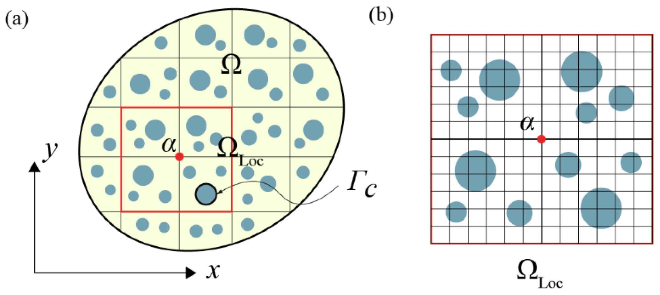
If one considers a 2D steady-state temperature field (Figure 2), with the absence of any heat source, solving the heat conduction problem is equivalent to minimizing the following function:
where T represents the temperature value, represents the thermal conductivity coefficient, represents the known heat flux, represents the known convective heat transfer coefficient, is the temperature of environment, and and are the boundaries on which the second and third boundary conditions are imposed, respectively.
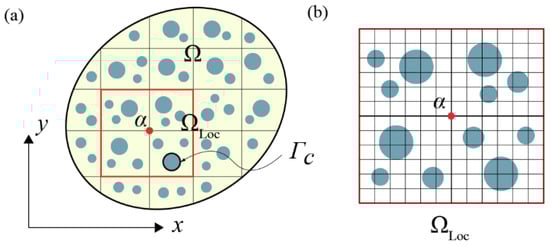
Figure 2.
(a) Computational domain and (b) two scale meshes.
The equilibrium expression in Equation (5) can be discretized by introducing the XFEM approximation. And applying the variation rule, the following discretized form is obtained:
where:
For a conventional node , the strain matrix takes the form of:
For an enriched node , the strain matrix takes the form of:
where is the total number of elements, and and are the total number of elements at which the second and third boundary conditions are applied, respectively. If two phases in the composites perfectly contact each other, the temperature and heat flux are continuous across the interface—this situation is referred to as the fourth boundary condition. And this boundary condition can be satisfied naturally with the interface enrichment function in Equation (2).
3. Framework and Implementation of GFEMgl
The generalized FEM with global–local enrichment (GFEMgl) is a more recent modification of the GFEM and designed to solve multiscale problems. It can be described as a two-scale approach which combines the GFEM and the global–local FEM. Early works on the GFEM relied on enrichment functions that contain a priori information extracted from the analytical solutions, such as linear fracturing, delamination of bimaterials, inclusions and voids, and heat and mass transfer in continuum media. However, in general, the analytical enrichments are not always available for the problems containing complicated subscale features. In such cases, the enrichment functions can be obtained from numerical solutions of auxiliary local partial differential equations (PDEs). The enrichment functions constructed in this manner are so-called global–local enrichments. In this method, these global–local enrichments are incorporated into the initial FEM approximation on a coarse mesh based on the PoU in a hierarchical manner; the coarse FEM approximation can capture global behavior, and these enrichments capture microscale details.
3.1. Implementation of GFEMgl
Based on partition of unity (PoU), The GFEMgl space is constructed by enriching an FE approximation space () with functions in the enriched space () in a hierarchical manner.
In this study, is discretized by bilinear quadrilateral elements and standard FE shape functions and α ∈ Ih = {1, 2, …, nn}, where α, Ih, and nn represent a node index, the set of all nodes, and the total number of nodes, respectively. The FE shape functions are used on the coarse mesh to span the global space, and these shape functions satisfy the following key property of PoU:
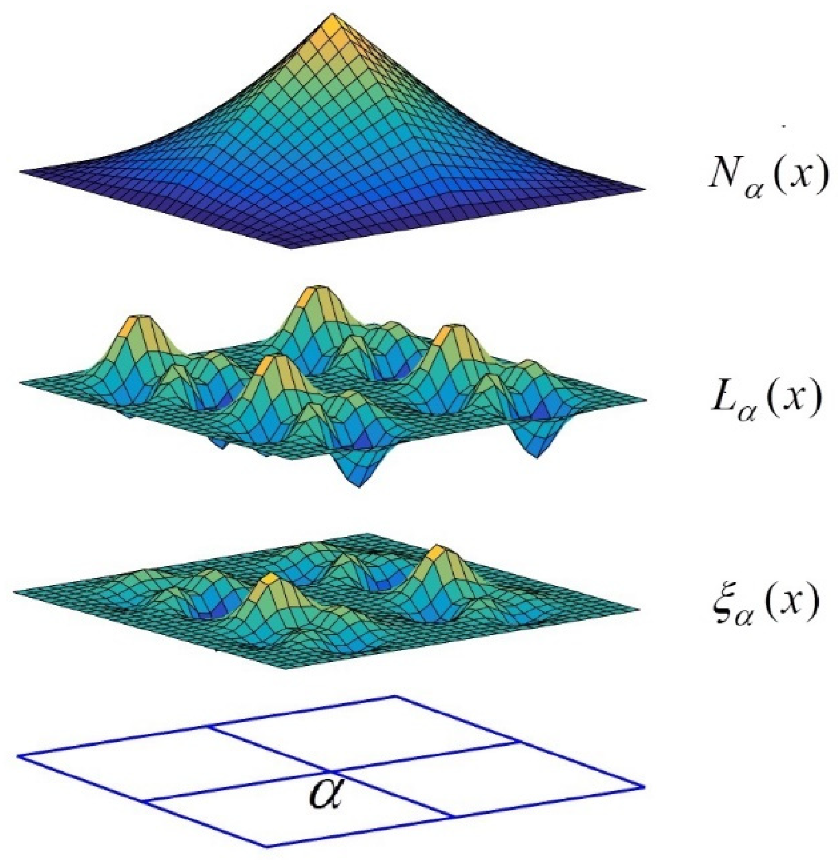
The enriched space is defined on a patch that comprises the set of elements sharing a common node covering the domain of interest. A GFEMgl shape function is obtained by multiplying an FE shape function with a global–local enrichment function as follows:
Figure 3 illustrates the patch and the GFEMgl shape function. Thus, the enriched space is spanned by ; i.e., . On the basis of these equations, the GFEMgl approximation of a scalar field can be expressed as follows:

Figure 3.
Illustration of a global–local enrichment function. is an FE interpolation function, is a global–local enrichment function, and is the resulting GFEMgl shape function.
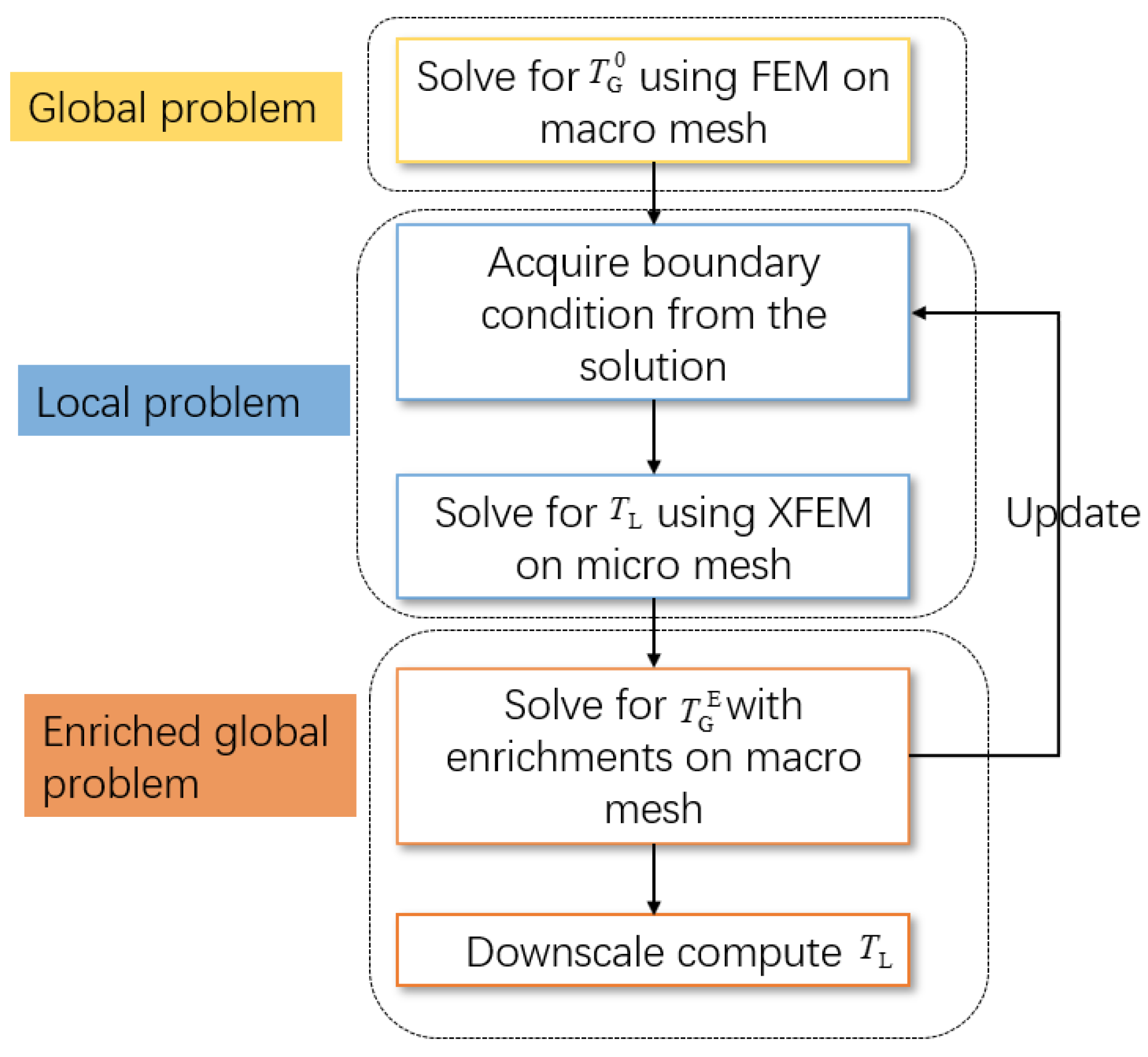
3.2. Computational Steps for Multiscale Simulation
Implementing the multiscale method requires combining three types of problems, i.e., the initial global problem, the local problems, and the enriched global problem.
For the initial global problem, a coarse mesh, regardless of the presence of micro-inclusions or voids, is generated. The solution space is discretized with standard FEM elements and shape functions. The solution of the initial global problem provides a crude estimation and is denoted as .
For a local problem, an auxiliary local problem is built by selecting all coarse FE elements sharing the vertex node , which compose a local domain (Figure 2). By subdividing each macro-element into micro-elements, a nested mesh is generated for the local problem. The micro-element size shall be sufficiently small to describe the geometry of inclusions or voids. In practice, the element size is typically set to one-fifth of the inclusion diameter. If the element size is too large, the geometric features of the inclusion or void cannot be accurately captured, thereby compromising integration precision. Conversely, excessively small element sizes lead to prohibitively high computational costs. For local problems, the XFEM is employed to model micro-discontinuities on a fine mesh. The boundary condition for the local problem is applied by the use of the coarse solution on corresponding micro-nodes. If one lets denote the XFEM solution of the local problem, it will be used as the global–local enrichment function. The global shape functions incorporated with the local solution can build a PoU.
The crude solution of the initial problem cannot provide detailed field variables on the fine scale, as it ignored the microstructure. However, the solution of a global problem enriched with global–local enrichments can reproduce accurate approximation. Multiple global–local iterations can be conducted to improve the quality of global–local enrichments. The numerical cases in this study indicate that the final solution is sufficiently accurate without any iteration.
For the enriched global problem, the numerically constructed enrichment functions are incorporated into the FEM approximation space of the coarse mesh based on the concept of PoU, as described in Equation (20). The global–local shape functions are defined as in Equation (19). The problem defined on the coarse mesh with space is called the enriched global problem, of which the solution is denoted as .
The approximation defined in Equation (20) reproduces the value of on the enriched node with , which means that the approximation is not an interpolation, and the standard FE parameter is not the real value on the enriched node . This scenario is problematic if a Dirichlet boundary condition is imposed on a boundary where the nodes happen to be enriched. A remedy for conventional GFEM approximation is to shift the global–local enrichment to 0 at node , thus obtaining the following expression:
Consequently, the temperature value on an enriched node is equal to the FE parameter .
Taking advantage of the nested meshes of two scales, the shifted global–local enrichment functions can be integrated into the global approximation space discretized on the coarse mesh. The integration order of each microscale element is selected as the maximum among integration orders of (i) the macroscale elements as required by the FEM or (ii) the microscale element as required by the XFEM plus 1. The integration order is increased by 1 to take into account the incorporated global–local enrichment function. This strategy accurately and efficiently provides integrity for the global–local enrichment functions.
In summary, the proposed GFEMgl involves solving the following three problems: (1) using the FEM to solve the initial global problem; (2) using the XFEM to solve the auxiliary local problem with local boundary conditions provided by the FEM solution; (3) solving the enriched global problem, in which global–local enrichments are added.
A flowchart of the presented multiscale algorithm is as follows (Figure 4):
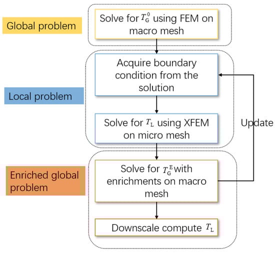
Figure 4.
A flowchart of the presented multiscale method combining GFEMgl and XFEM.
4. Numerical Cases and Discussion
To illustrate the accuracy and versatility of the proposed multiscale method, several numerical cases are conducted, and the ETC is evaluated on the base of the temperature results. The results are compared with those obtained from the standard XEFM and analytical method. In order to predict the ETC accurately, an RVE is generated with a large number of randomly distributed non-overlapping circular inclusions or voids. The influences of different populations and sizes of the inclusions or voids are investigated. In this study, the inclusions and voids are restricted to a circular shape. For inclusions and voids with irregular shapes, the complex geometry can be easily broken down by 2D or 3D triangulation. Combined with Boolean operations, the geometries can be located by the use of the level set method.
4.1. XFEM Simulation of Two Inclusions/Voids
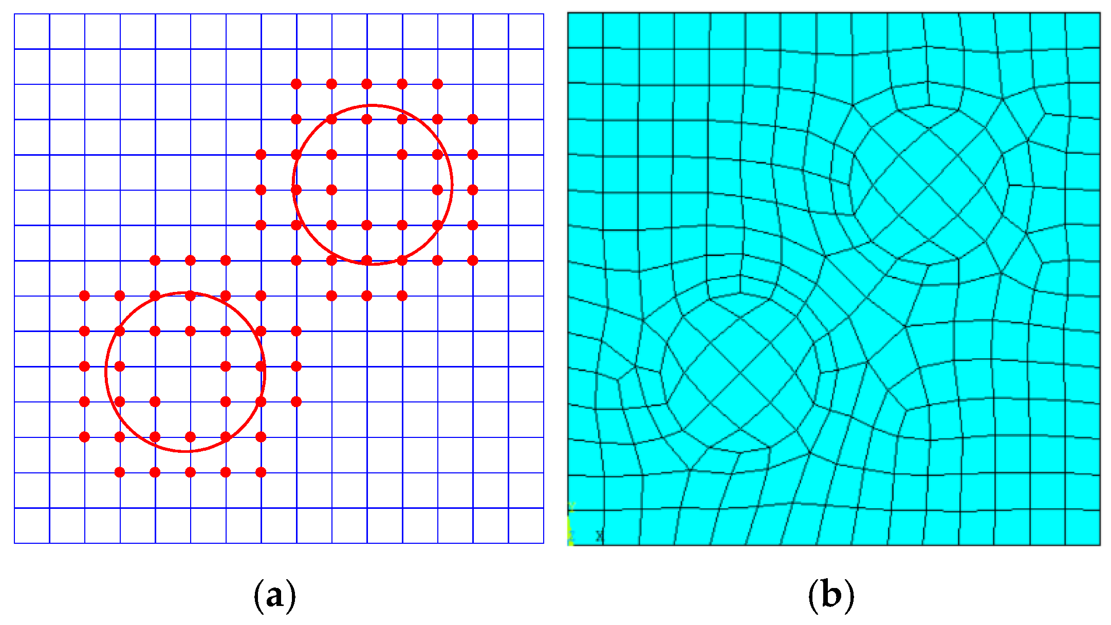
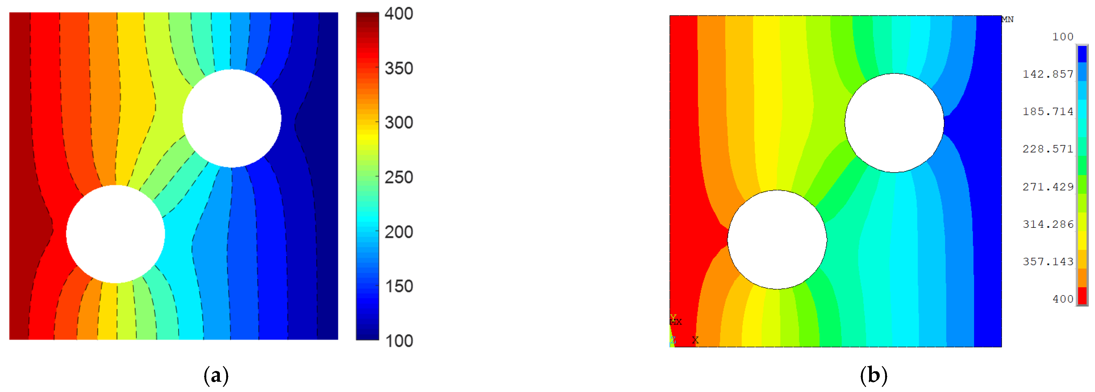
To validate the XFEM for a temperature field, a square plate containing two circular inclusions was numerically simulated by the XFEM and FEM, and the obtained results were compared. The size of the plate was 10 × 10 m, and the radius of each inclusion was 1.5 m. The configuration of two inclusions is visible in the XFEM and FEM mesh shown in Figure 5. The temperatures of the left and right edges were set to be 400 and 100 °C, respectively, and the top and bottom edges were kept as adiabatic surfaces. The thermal conductivity coefficient of the inclusions and matrix were set as 1000 and 100 kJ/(m·h·°C), respectively.
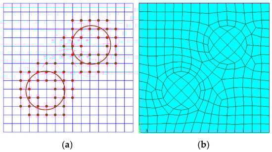
Figure 5.
Meshes used for the (a) XFEM and (b) FEM. The red dots indicate enriched nodes (The red circles mark the two inclusions).
The XFEM solution was implemented in MATLAB® (The MathWorks Inc. version: 9.13.0 R2022b) and the FEM solution was performed using ANSYS®Workbench™ (version 16.0). In both methods, the same element size was adopted to enable comparison. As shown in Figure 5, the mesh in the XFEM analysis is independent of the geometry of the material interfaces. In contrast, the mesh required by the FEM must conform to the physical boundaries of inclusions. The XFEM meshing generates 255 elements and 256 nodes, and FEM meshing generates 234 elements and 265 nodes.
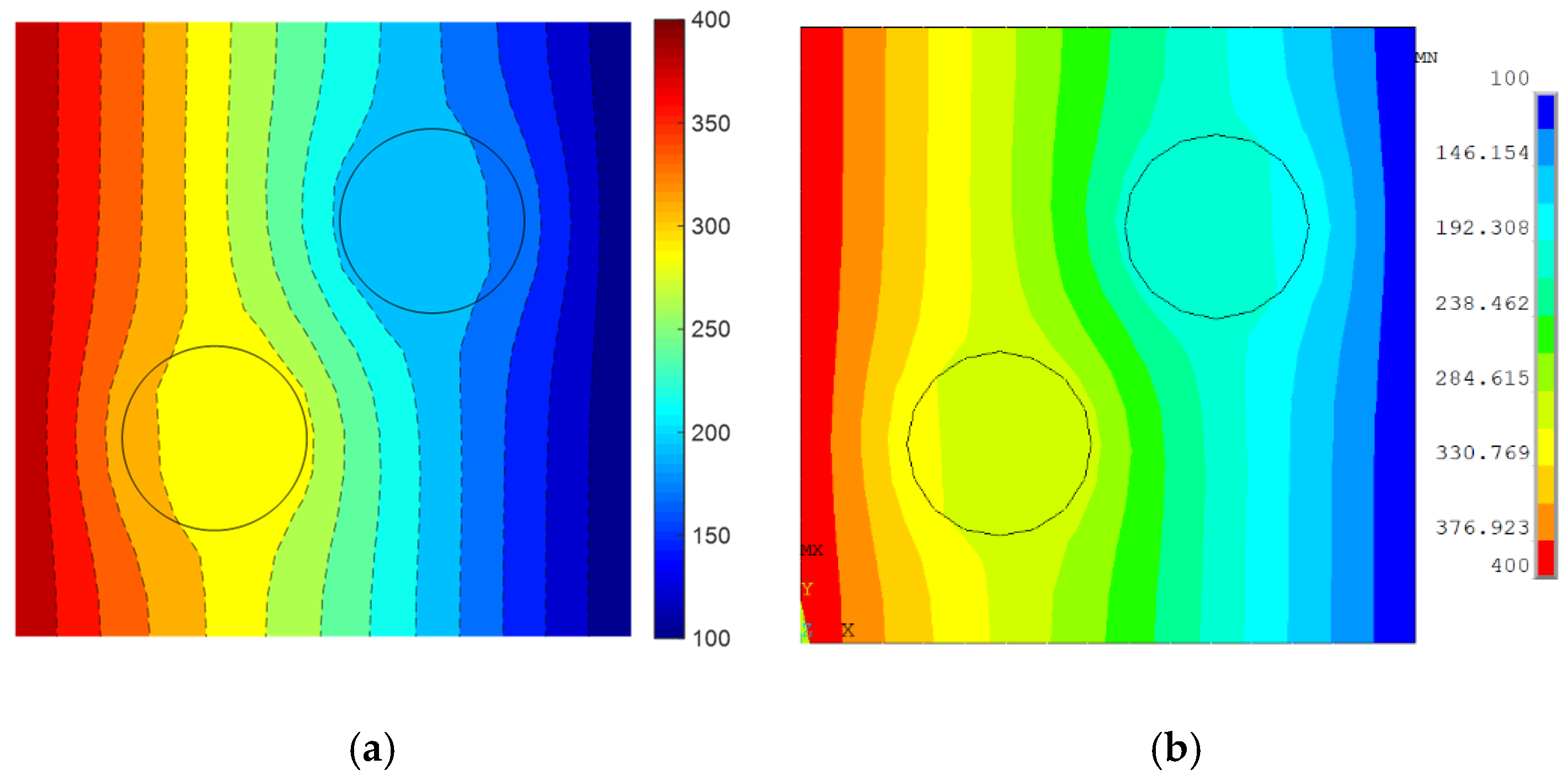
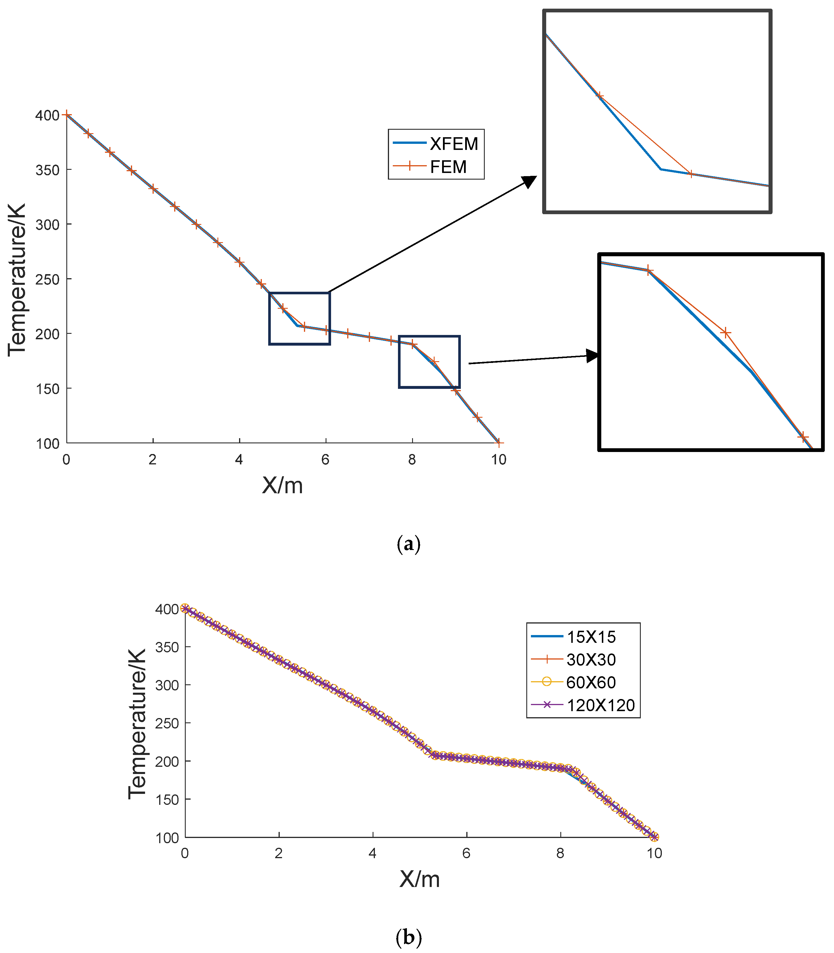
Contour plots of temperature results by the two methods are presented in Figure 6. In order to compare the results of the two methods, the temperature variation curves along y = 6.66667 m (the center of the upper inclusion) are plotted in Figure 7a. With a coarse mesh in the XFEM, only a minimal difference can be found around the interfaces between the matrix and inclusion. The mesh resolution was investigated by using four different meshes that consist of 15 × 15, 30 × 30, 60 × 60, and 120 × 120 elements, respectively. The temperature distribution at y = 6.66667 m produced by these meshes is plotted in Figure 7b. It indicates that mesh refinement had a minimal effect on the XFEM results; even the coarsest mesh produced an accurate result. At its smallest, the element size should be sufficiently small to describe the geometry of heterogeneities.

Figure 6.
Temperature profiles for a plate with two inclusions obtained from the (a) XFEM and (b) FEM.
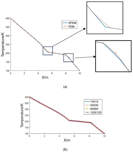
Figure 7.
Temperature values obtained along y = 6.66667 m obtained by (a) XFEM vs. FEM and (b) XFEM with different mesh densities.
In practice, voids within composites are filled with air, which has considerably low thermal conductivity. Voids in numerical simulations can either be modeled by treating them as inclusions with thermal conductivity that is relatively much lower, or they can be modeled with the XFEM approximation presented in Equation (4), in which the boundary of a void is actually set as adiabatic. In practice, instead of incorporating the void enrichment , the enriched elements are divided into sub-triangles conformal to interfaces and integration points where (i.e., inside the voids) are simply excluded.
To simulate the plate with voids, the second method was employed to showcase the effectiveness of XFEM. For this case, the contour plots of the temperature fields obtained from the XFEM and FEM are depicted in Figure 8 for comparison; these fields have favorable agreement.
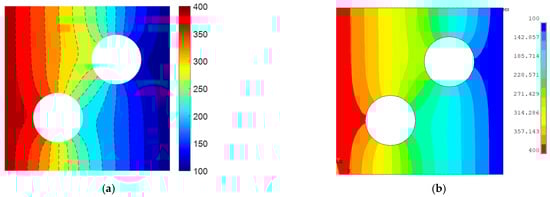
Figure 8.
Comparison of the temperature result in x-direction for the plate with two voids obtained from the (a) XFEM and (b) FEM. The white circles mark the two inclusions.
4.2. GFEMgl Simulation of RVEs with Inclusions
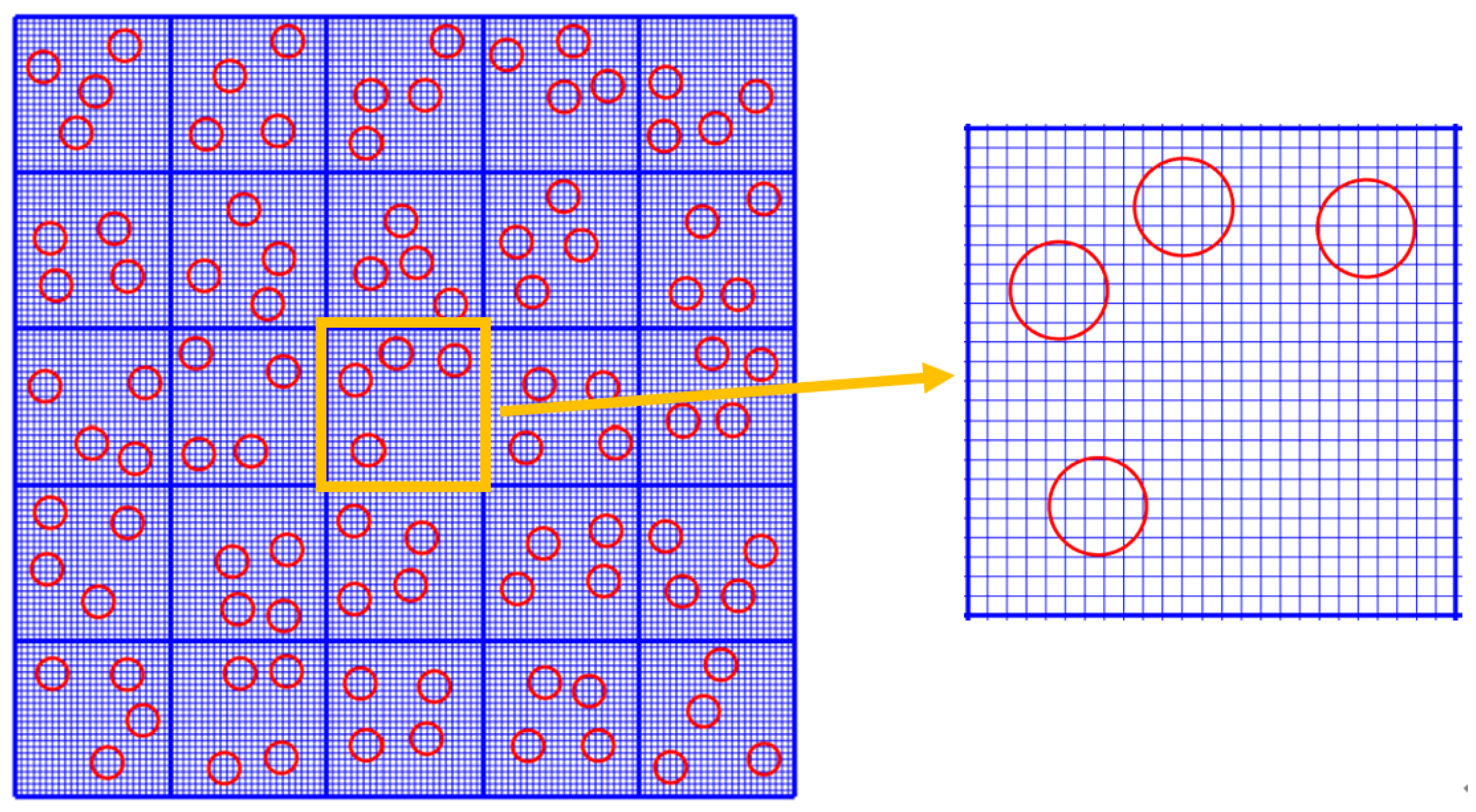
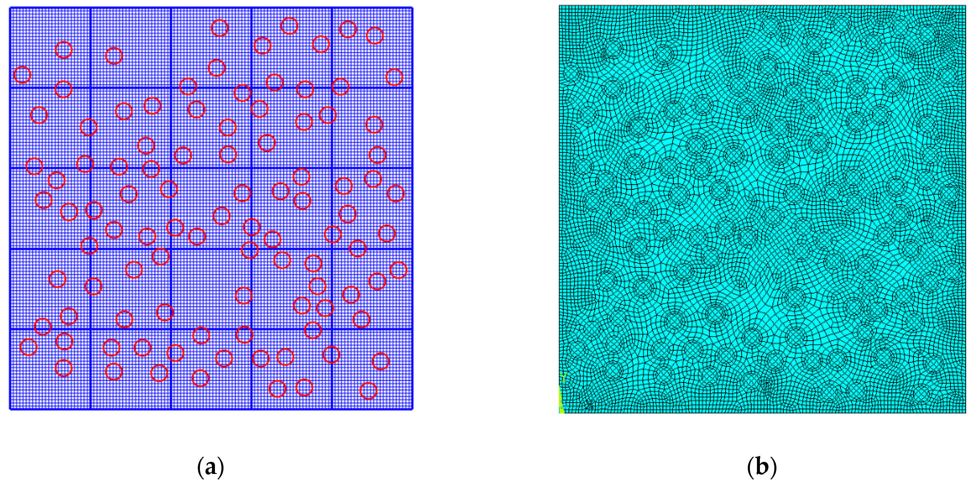
An RVE containing randomly distributed inclusions was simulated using the proposed multiscale method to demonstrate the effectiveness of the proposed multiscale approach. An RVE should be properly configured to effectively reflect the material microstructure; that is, both the domain size and number of inclusions should be adequate. The considered RVE was discretized with a 5 × 5 grid of macro-elements, and each macro-element contained four randomly distributed non-overlapping inclusions. Therefore, the RVE had a total of 100 inclusions; the configuration of the RVE and two scale meshes are shown in Figure 9. Each macro-element was further discretized into a 25 × 25 grid of micro-elements.
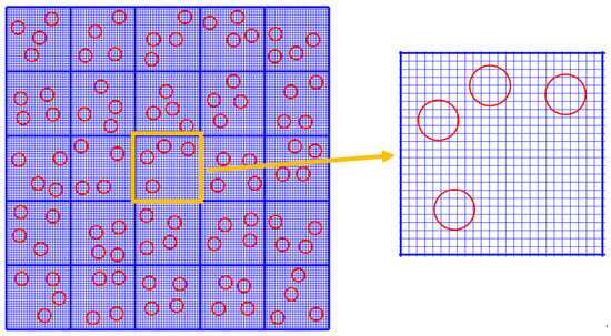
Figure 9.
Macro- and micro-meshes of an RVE containing 100 randomly distributed inclusions.
The RVE size was set as 50 × 50 m2, and all inclusions had a uniform radius of R = 1 m. The volume fraction of inclusions in this configuration was therefore 12.95%. The thermal conductivity coefficients of the matrix and inclusions were set as 10 and 100 kJ/(m·h·°C), respectively. Moreover, the temperatures of the left and right edges were set as 400 and 100 °C, respectively, and the top and bottom edges were set as adiabatic surfaces.
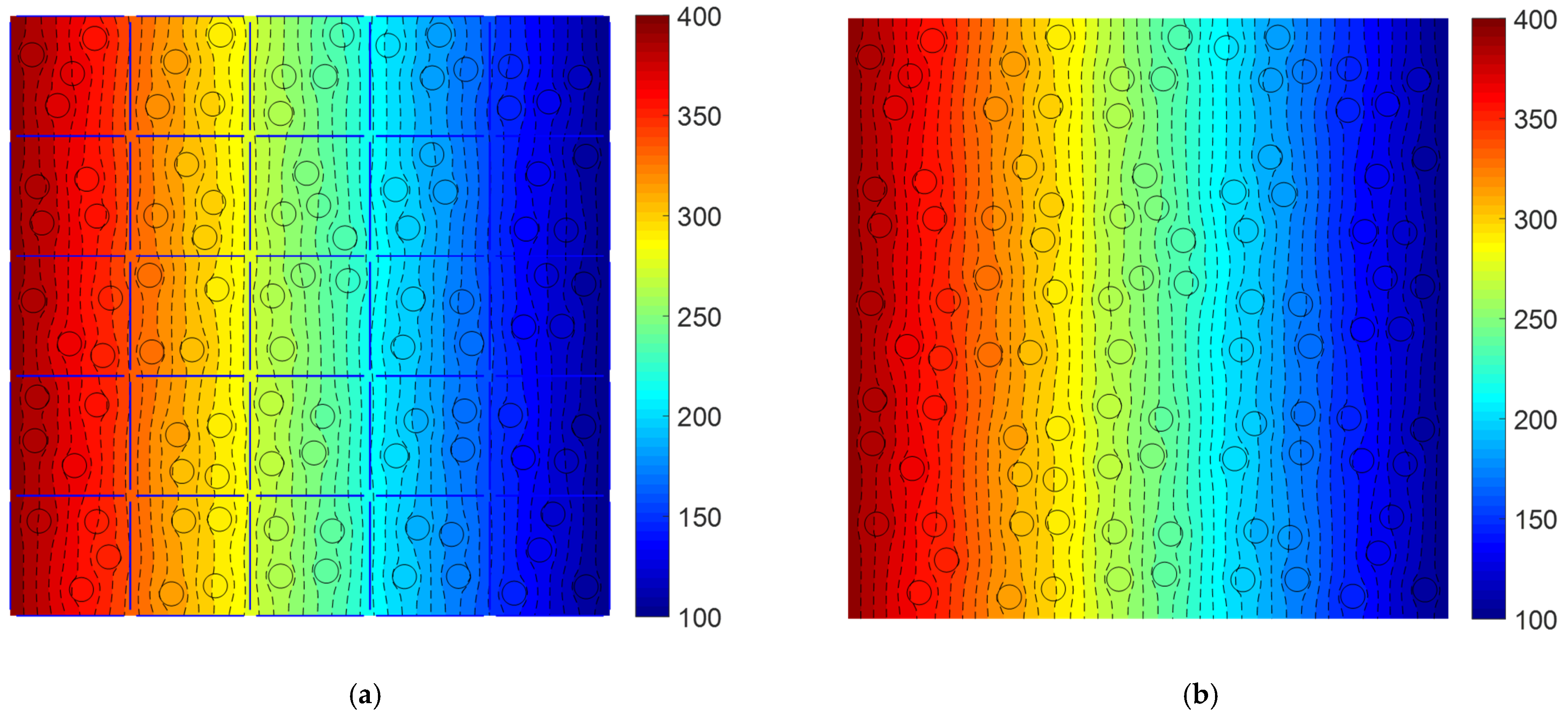
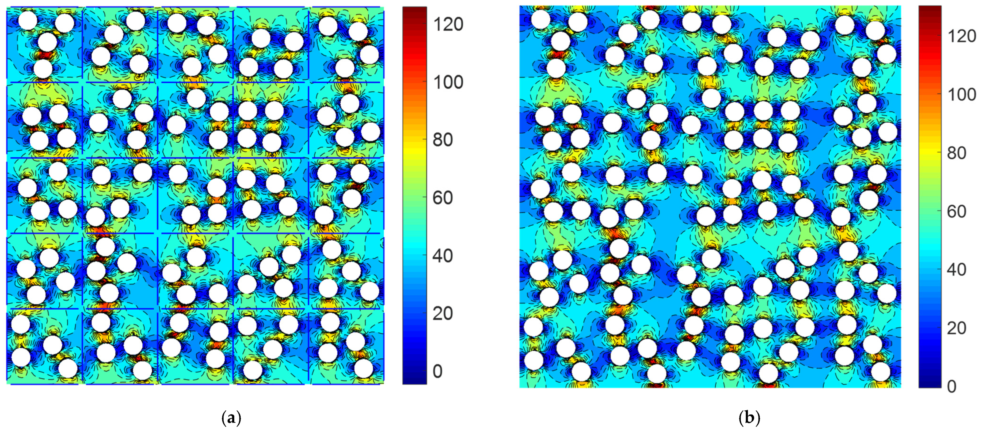
To compare the CPU time and to examine the effectiveness of the proposed multiscale method, the considered configuration was also solved using standard single-scale XFEM, where the elements’ size was set to be the same as that of the micro-elements in the proposed multiscale method. The temperature results obtained from the two methods are provided as contour plots in Figure 10. In the contour plots, the blue dashed lines mark the boundaries of the macro-elements, and the black dashed lines are isothermal lines. The results of the proposed GFEMgl and the XFEM are in good agreement; minimal differences were observed only at the peripheries of certain inclusions. Both algorithms are implemented in MATLAB software on the same computer (CPU @2.90GHz dual-core, RAM of 32.0 GB). The proposed GFEMgl required 51 s to solve this case, whereas the standard XFEM required 121.2 s. It should be noted that the runtime gap is produced by the specific configurations. When the scale difference becomes larger, more macro-elements are generated in the coarse mesh, and the runtime gap could be more significant.
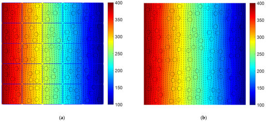
Figure 10.
Comparison of temperature field of multiple inclusions obtained from (a) the proposed GFEMgl and (b) standard XFEM.
4.3. Influence of Volume Fraction of Inclusions on ETC
To investigate the influence of the volume fraction of inclusions on the ETC, detailed thermal conduction analyses were carried out first on an RVE. For all configurations considered in this subsection, a constant temperature of 400 and 100 °C were set for the left and right edges, respectively, and the other two edges were kept adiabatic. The same RVE and thermal properties described in Section 4.2 were also employed for the computations conducted in this subsection. The effective heat flux of the composites along the direction of heat transfer can be calculated by the integration over the entire domain. The ETC in the x-direction can thus be calculated based on Fourier’s law as follows:
where denotes the total heat flux along the x-direction, denotes the distance between two opposite boundaries, and are the temperatures applied on two opposite boundaries, and denotes the ETC of the composite in the x-direction. Because the constituents considered in this study are isotropic, the resulting is isotropic.
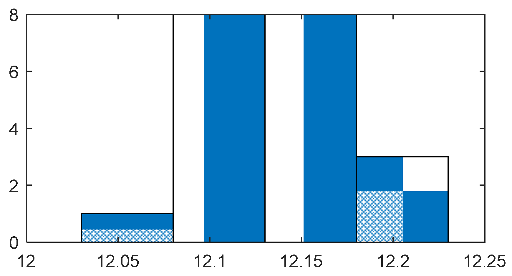
To investigate the influence of the randomness of the inclusion distribution, an inclusion configuration similar to that shown in Figure 10 was randomly generated 20 times, and the ETC was calculated for each configuration test. A histogram of the estimated ETC for these tests is depicted in Figure 11. The obtained ETC values had a small range of 12.05–12.20 kJ/(m·h·°C), and the variance of these 20 data was 0.0012 kJ/(m·h·°C). These results suggest that the randomness of the inclusion distribution has a minor influence on the overall thermal properties of a composite.

Figure 11.
Histogram of the ETC for different random configurations of inclusion configurations.
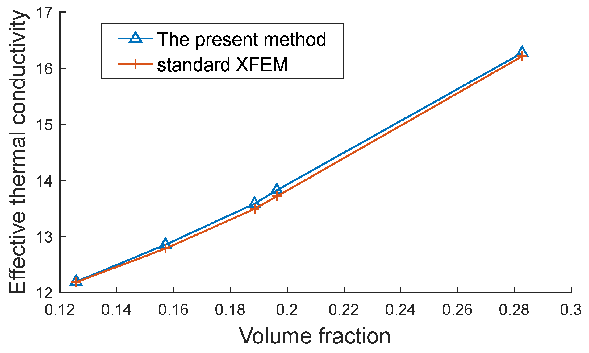
The volume fraction of the inclusions was varied by changing the inclusion radius or the total number of inclusions. The inclusions in the RVE are of uniform radius and randomly distributed. Three radii were, i.e., r = 1, 1.25, or 1.5 m, and the corresponding volume fractions were 12.6%, 19.6%, or 28.3%, respectively. For the same RVE, the total number of inclusions was varied as 100, 125, or 150, and the corresponding volume fractions were 12.6%, 15.7%, or 18.9%, respectively. The ETC results obtained by different approaches are listed in Table 1.

Table 1.
ETC results [unit: kJ/(m·h·°C)] obtained with different methods for numerous inclusions.
The numerical results obtained using the proposed multiscale method were compared with those obtained using the standard XFEM and an analytical model, i.e., the parallel-series (P–S) bound model. In this analytical model, the ETC of a composite is provided by an upper bound, which is calculated by the volume fraction weighted series, and a lower bound which is calculated by parallel average, as follows:
where and are the thermal conductivities of the inclusions and matrix, respectively. The ETC values obtained using the proposed GFEMgl are in good agreement with those obtained using the standard XFEM. As expected, the numerical results lie between the upper and lower bounds of the P–S model but closer to the P bound, which is known to provide a better estimation of the ETC than does the S bound. The variation in the ETC with the volume fraction of inclusions is plotted in Figure 12. As expected, this relation was slightly nonlinear.
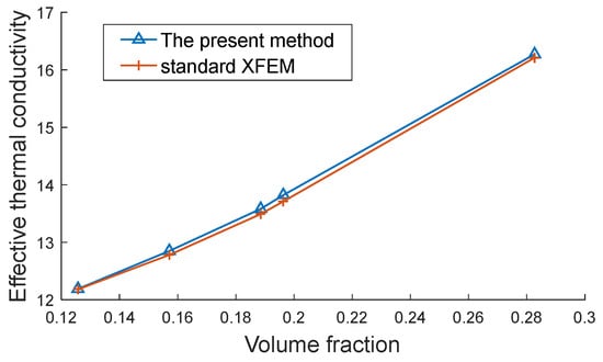
Figure 12.
Variation in the ETC [unit: kJ/(m·h·°C)] with the volume fraction of inclusions.
4.4. GFEMgl Simulation of RVEs with Voids
An RVE containing circular voids was simulated using the proposed GFEMgl. The size of the RVE and the configuration of the voids were assigned the same values as in the previous case with inclusions. The thermal conductivity coefficient of the matrix was set as 10 kJ/(m·h·°C), and the boundary conditions were the same as in the previous cases. The void arrangement was varied in the same manner as described in Section 4.3.
The results obtained with the proposed GFEMgl and the standard XFEM were compared for the configuration with r = 1.25 m and Num = 100 as an example. The contour plots of thermal flux in the x-direction are displayed in Figure 13. The thermal flux results obtained with the proposed GFEMgl are almost identical to those obtained with standard XFEM, even on the boundaries of the macro-elements. Both algorithms were implemented in MATLAB software on the same computer, with the GFEMgl requiring 19.5 s to solve this case, while the standard XFEM required 51.2 s. Because the void enrichment is easier to implement and introduces no additional degree of freedom, the problems with voids demand lower computational time as compared with those with inclusions. Likewise, the proposed multiscale method resulted in a considerable reduction in computational time compared with the standard XFEM.
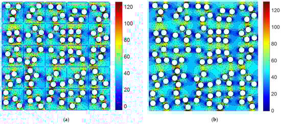
Figure 13.
Thermal flux results in the x-direction produced by the (a) proposed GFEMgl and (b) standard XFEM.
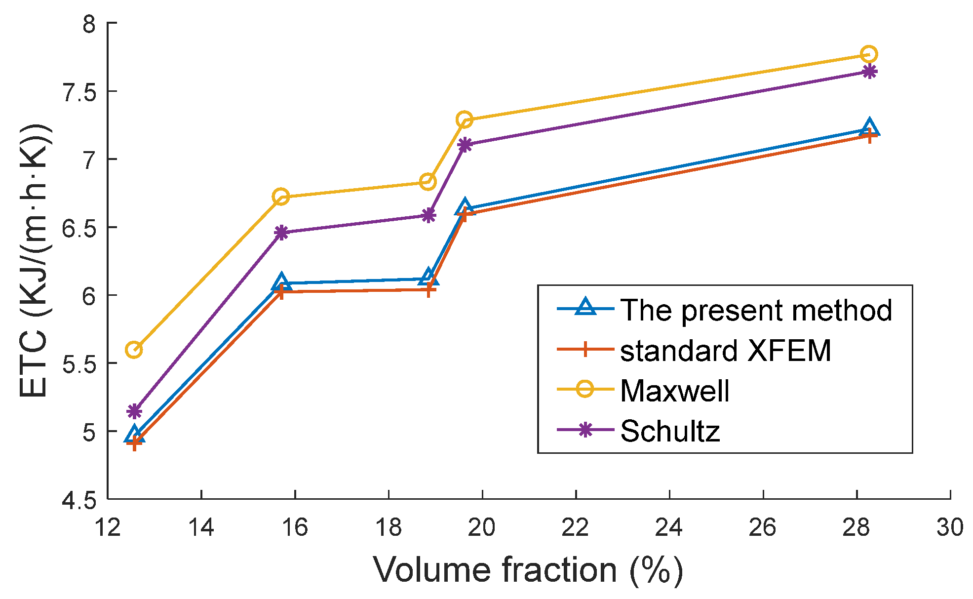
The ETC was calculated after the numerical simulation of the temperature field and compared with that evaluated by the following analytical models: the Maxwell model and Schultz model. These models are commonly used to estimate heat transfer in porous media. The Maxwell and Schultz models are expressed in the following equations, respectively:
where denotes the porosity of the voids in the composite.
The ETC results are presented in Table 2. The ETC results obtained using the proposed GFEMgl agree well with those obtained using the standard XFEM. Moreover, the ETC values obtained using the GFEMgl are more similar to those obtained by the Schultz model as compared with the Maxwell model. The variation in the estimated ETC with the volume fraction of voids is plotted in Figure 14. The curves have a similar trend for all the methods. It should be noted that the analytical models only provide a quick and rough estimation of the ETC, and the numerical simulation methods were typically more accurate than those models.
Table 2.
ETC results [unit: kJ/(m·h·°C)] obtained with various methods for numerous voids.
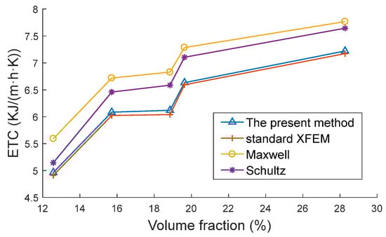
Figure 14.
Variation in ETC with volume fraction of voids.
4.5. An RVE with 100 Randomly Distributed Inclusions
In order to examine the versatility of the proposed method in simulating inclusions randomly distributed over the whole domain, the constraint whereby a certain number of inclusions be contained within each macro-element was removed. A total of 100 inclusions, each with a uniform radius of 1.0 m, were randomly distributed over an RVE of 50 × 50 m2. The thermal conductivity coefficient of the matrix and inclusions were set as 10 kJ/(m·h·°C) and 100 kJ/(m·h·°C), respectively, and the boundary conditions were the same as those described in the previous cases.
This configuration is also solved in ANSYS with the same element size (h = 0.4 m) for comparison. In total, 10,402 elements are discretized in ANSYS, while the structured mesh of the present method generates 15,625 elements. A great deal of computation time was spent to make the FEM mesh. A comparison of the meshes can be seen in Figure 15.
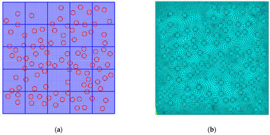
Figure 15.
Meshes generated by (a) the presented method (b) FEM in ANSYS.
In order to remove the constraint that inclusions are contained within macro-elements, which means the interfaces of inclusions may intersect with the macro-elements’ boundaries, additional programming effort is required to identify and include those inclusions that intersect with macro-element boundaries when calculating the level set function values at all micro-nodes. Contour plots of the temperature field are provided in Figure 16, in which the range [100 400] is divided into 25 uniform contour levels. A good agreement can be found between the temperature results. Even when the enrichments are located on the boundaries of macro-elements, the temperature result is continuous over the entire domain.
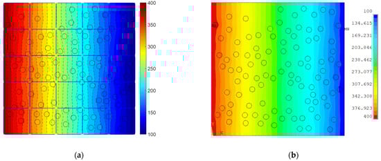
Figure 16.
Comparison of temperature contour plots of 100 randomly distributed inclusions obtained from (a) the proposed GFEMgl and (b) FEM in ANSYS.
5. Conclusions
This work presents a novel GFEMgl scheme for modeling the temperature field in composite materials containing randomly distributed inclusions or voids. Then, ETC is calculated on the basis of detailed numerical simulation of an RVE. In the proposed method, the XFEM was employed on the micro-mesh to avoid using conformal mesh with discontinuities. Global–local enrichments are numerically constructed and then incorporated into a global approximation to integrate microstructure information. A shifted modification of global–local enrichment is proposed herein to facilitate boundary conditions in multiscale homogenization problems. Multiple numerical cases were solved in this study to examine the effectiveness of the proposed method. The following conclusions were obtained on the basis of the results acquired for these cases.
- The results of XFEM simulations of a plate with inclusions or voids agree well with those of FEM simulations in terms of temperature and thermal flux. The XFEM enables simulation to be conducted on a structured mesh, while maintaining high accuracy.
- The results produced by the proposed multiscale method are in favorable agreement with those produced by the standard single-scale XFEM, and the results fit in the bounds produced by the P-S model. However, the proposed method is more computationally efficient than the standard XFEM for composites with numerous heterogeneities.
- The randomness of the inclusion distribution does not notably affect the overall thermal property of a composite.
- ETC has an approximately linear relationship with the volume fraction of composites containing inclusions; however, ETC has a nonlinear relationship with the porosity of porous composites. The numerical ETC results obtained with the proposed method are closer to those produced by the Schultz model than to those produced by the Maxwell model.
The numerical applications of the presented multiscale method are limited to circular-shaped inclusions and voids. Irregularly shaped inclusions can also be handled by developing the level set method to track the complex geometries. The developed method also has great potential to be extended to transient heat transfer problems, in which the mass matrices should be upscale computed in a similar manner as the thermal conductivity matrices. In addition, the present method is expected to be extended to the three-dimension domain in future work. Finally, the convergence of this multiscale method requires further study.
Author Contributions
Methodology, G.L.; Software, Y.B.; Validation, J.G.; Writing—original draft, G.L.; Writing—review & editing, H.P. All authors have read and agreed to the published version of the manuscript.
Funding
The support of the National Natural Science Foundation of China (Nos. 51909153, 52278190, and 12372270) is gratefully acknowledged.
Data Availability Statement
The original contributions presented in this study are included in the article. Further inquiries can be directed to the corresponding author.
Conflicts of Interest
The authors declare no conflicts of interest.
References
- Kaur, I.; Mahajan, R.L.; Singh, P. Generalized correlation for effective thermal conductivity of high porosity architectured materials and metal foams. Int. J. Heat Mass Transf. 2023, 200, 123512. [Google Scholar]
- Wang, J.; Carson, J.K.; North, M.F.; Cleland, D.J. A new approach to modelling the effective thermal conductivity of heterogeneous materials. Int. J. Heat Mass Transf. 2006, 49, 3075–3083. [Google Scholar]
- Kiradjiev, K.B.; Halvorsen, S.A.; Van Gorder, R.A.; Howison, S.D. Maxwell-type models for the effective thermal conductivity of a porous material with radiative transfer in the voids. Int. J. Therm. Sci. 2019, 145, 106009. [Google Scholar]
- Zerhouni, O.; Tarantino, M.G.; Danas, K. Numerically-aided 3D printed random isotropic porous materials approaching the Hashin-Shtrikman bounds. Compos. Part B Eng. 2019, 156, 344–354. [Google Scholar]
- Back, S.Y.; Mori, T.; Rhyee, J.-S. Thermoelectric properties and effective medium theory analysis on the (GeTe)1-x(InTe)x composites. J. Alloys Compd. 2024, 1002, 175316. [Google Scholar]
- Bi, J.; Zhang, M.; Chen, W.; Lu, J.; Lai, Y. A new model to determine the thermal conductivity of fine-grained soils. Int. J. Heat Mass Transf. 2018, 123, 407–417. [Google Scholar] [CrossRef]
- Ranut, P. On the effective thermal conductivity of aluminum metal foams: Review and improvement of the available empirical and analytical models. Appl. Therm. Eng. 2016, 101, 496–524. [Google Scholar]
- Cook, R.D.; Malkus, D.S.; Plesha, M.E.; Witt, R.J. Concepts and Applications of Finite Element Analysis; John Wiley & Sons: Hoboken, NJ, USA, 2002. [Google Scholar]
- Mendes, M.A.A.; Ray, S.; Trimis, D. A simple and efficient method for the evaluation of effective thermal conductivity of open-cell foam-like structures. Int. J. Heat Mass Transf. 2013, 66, 412–422. [Google Scholar]
- Yang, M.; Li, X. Optimum convergence parameters of lattice Boltzmann method for predicting effective thermal conductivity. Comput. Methods Appl. Mech. Eng. 2022, 394, 114891. [Google Scholar]
- Shen, Y.-L.; Abdo, M.G.; Van Rooyen, I.J. Numerical Study of Effective Thermal Conductivity for Periodic Closed-Cell Porous Media. Transp. Porous Media 2022, 143, 245–269. [Google Scholar]
- Li, Z.; Yang, Y.; Gariboldi, E.; Li, Y. Computational models of effective thermal conductivity for periodic porous media for all volume fractions and conductivity ratios. Appl. Energy 2023, 349, 121633. [Google Scholar] [CrossRef]
- Sukumar, N.; Chopp, D.L.; Moës, N.; Belytschko, T. Modeling holes and inclusions by level sets in the extended finite-element method. Comput. Methods Appl. Mech. Eng. 2001, 190, 6183–6200. [Google Scholar] [CrossRef]
- Moës, N.; Belytschko, T. Extended finite element method for cohesive crack growth. Eng. Fract. Mech. 2002, 69, 813–833. [Google Scholar] [CrossRef]
- Moës, N.; Cloirec, M.; Cartraud, P.; Remacle, J.F. A computational approach to handle complex microstructure geometries. Comput. Methods Appl. Mech. Eng. 2003, 192, 3163–3177. [Google Scholar] [CrossRef]
- Heidari-Rarani, M.; Sayedain, M. Finite element modeling strategies for 2D and 3D delamination propagation in composite DCB specimens using VCCT, CZM and XFEM approaches. Theor. Appl. Fract. Mech. 2019, 103, 102246. [Google Scholar] [CrossRef]
- Yu, T.T.; Gong, Z.W. Numerical simulation of temperature field in heterogeneous material with the XFEM. Arch. Civ. Mech. Eng. 2013, 13, 199–208. [Google Scholar] [CrossRef]
- Zamani, A.; Eslami, M.R. Implementation of the extended finite element method for dynamic thermoelastic fracture initiation. Int. J. Solids Struct. 2010, 47, 1392–1404. [Google Scholar] [CrossRef]
- Mora, D.F.; Niffenegger, M. A new simulation approach for crack initiation, propagation and arrest in hollow cylinders under thermal shock based on XFEM. Nucl. Eng. Des. 2022, 386, 111582. [Google Scholar] [CrossRef]
- Svenning, E.; Fagerström, M.; Larsson, F. On computational homogenization of microscale crack propagation. Int. J. Numer. Methods Eng. 2016, 108, 76–90. [Google Scholar] [CrossRef]
- Song, J.-H.; Yoon, Y.-C. Multiscale failure analysis with coarse-grained micro cracks and damage. Theor. Appl. Fract. Mech. 2014, 72, 100–109. [Google Scholar] [CrossRef]
- Aduloju, S.C.; Truster, T.J. A variational multiscale discontinuous Galerkin formulation for both implicit and explicit dynamic modeling of interfacial fracture. Comput. Methods Appl. Mech. Eng. 2019, 343, 602–630. [Google Scholar]
- Mergheim, J. A variational multiscale method to model crack propagation at finite strains. Int. J. Numer. Methods Eng. 2009, 80, 269–289. [Google Scholar]
- Wu, J.; Zhang, H.; Zheng, Y. A concurrent multiscale method for simulation of crack propagation. Acta Mech. Solida Sin. 2015, 28, 235–251. [Google Scholar]
- Patil, R.U.; Mishra, B.K.; Singh, I.V. A multiscale framework based on phase field method and XFEM to simulate fracture in highly heterogeneous materials. Theor. Appl. Fract. Mech. 2019, 100, 390–415. [Google Scholar] [CrossRef]
- Zhang, H.W.; Wu, J.K.; Lv, J. A new multiscale computational method for elasto-plastic analysis of heterogeneous materials. Comput. Mech. 2011, 49, 149–169. [Google Scholar]
- Liu, G.; Guo, J.; Bao, Y. A New Multiscale XFEM with Projection Method for Interaction between Macrocrack and Microcracks. Eng. Fract. Mech. 2023, 285, 109286. [Google Scholar] [CrossRef]
- Deng, H.; Yan, B.; Okabe, T. Fatigue crack propagation simulation method using XFEM with variable-node element. Eng. Fract. Mech. 2022, 269, 108533. [Google Scholar]
- Ding, J.; Yu, T.; Bui, T.Q. Modeling strong/weak discontinuities by local mesh refinement variable-node XFEM with object-oriented implementation. Theor. Appl. Fract. Mech. 2020, 106, 102434. [Google Scholar] [CrossRef]
- Teng, Z.H.; Liao, D.M.; Wu, S.C.; Sun, F.; Chen, T.; Zhang, Z.B. An adaptively refined XFEM for the dynamic fracture problems with micro-defects. Theor. Appl. Fract. Mech. 2019, 103, 102255. [Google Scholar]
- Duarte, C.A.; Kim, D.J. Analysis and applications of a generalized finite element method with global–local enrichment functions. Comput. Methods Appl. Mech. Eng. 2008, 197, 487–504. [Google Scholar]
- Wang, X.; Chung, E.; Fu, S.; Huang, Z. Mixed GMsFEM for linear poroelasticity problems in heterogeneous porous media. J. Comput. Appl. Math. 2021, 390, 102255. [Google Scholar]
- Pereira, J.P.A.; Kim, D.J.; Duarte, C.A. A two-scale approach for the analysis of propagating three-dimensional fractures. Comput. Mech. 2011, 49, 99–121. [Google Scholar]
- Plews, J.; Duarte, C.A.; Eason, T. An improved nonintrusive global–local approach for sharp thermal gradients in a standard FEA platform. Int. J. Numer. Methods Eng. 2012, 91, 426–449. [Google Scholar]
- He, L.; Valocchi, A.J.; Duarte, C.A. An adaptive global–local generalized FEM for multiscale advection–diffusion problems. Comput. Methods Appl. Mech. Eng. 2024, 418, 116548. [Google Scholar]
- Kim, J.; Simone, A.; Duarte, C.A. Mesh refinement strategies without mapping of non-linear solutions for the generalized and standard FEM analysis of 3-D cohesive fractures. Int. J. Numer. Methods Eng. 2015, 109, 235–258. [Google Scholar]
- Plews, J.A.; Duarte, C.A. A two-scale generalized finite element approach for modeling localized thermoplasticity. Int. J. Numer. Methods Eng. 2016, 108, 1123–1158. [Google Scholar]

Disclaimer/Publisher’s Note: The statements, opinions and data contained in all publications are solely those of the individual author(s) and contributor(s) and not of MDPI and/or the editor(s). MDPI and/or the editor(s) disclaim responsibility for any injury to people or property resulting from any ideas, methods, instructions or products referred to in the content. |
© 2025 by the authors. Licensee MDPI, Basel, Switzerland. This article is an open access article distributed under the terms and conditions of the Creative Commons Attribution (CC BY) license (https://creativecommons.org/licenses/by/4.0/).